High-order Moment Closure Models with Random Batch Method for Efficient Computation of Multiscale Turbulent Systems

Abstract

We propose a high-order stochastic-statistical moment closure model for efficient ensemble prediction of leading-order statistical moments and probability density functions in multiscale complex turbulent systems. The statistical moment equations are closed by a precise calibration of the high-order feedbacks using ensemble solutions of the consistent stochastic equations, suitable for modeling complex phenomena including non-Gaussian statistics and extreme events. To address challenges associated with closely coupled spatio-temporal scales in turbulent states and expensive large ensemble simulation for high-dimensional systems, we introduce efficient computational strategies using the random batch method (RBM). This approach significantly reduces the required ensemble size while accurately capturing essential high-order structures. Only a small batch of small-scale fluctuation modes is used for each time update of the samples, and exact convergence to the full model statistics is ensured through frequent resampling of the batches during time evolution. Furthermore, we develop a reduced-order model to handle systems with really high dimension by linking the large number of small-scale fluctuation modes to ensemble samples of dominant leading modes. The effectiveness of the proposed models is validated by numerical experiments on the one-layer and two-layer Lorenz ’96 systems, which exhibit representative chaotic features and various statistical regimes. The full and reduced-order RBM models demonstrate uniformly high skill in capturing the time evolution of crucial leading-order statistics, non-Gaussian probability distributions, while achieving significantly lower computational cost compared to direct Monte-Carlo approaches. The models provide effective tools for a wide range of real-world applications in prediction, uncertainty quantification, and data assimilation.

1 Introduction

Turbulent dynamical systems encountered in science and engineering [24, 34, 31, 19] exhibit distinguished characteristics including a high-dimensional state space with multiple spatio-temporal scales and strong internal instabilities [11, 25]. Forecasting the intricate behaviors of such complex systems poses a significant challenge in uncertainty quantification and data assimilation problems [39, 28, 29, 3]. One key aspect involves accurately quantifying the multiscale interaction between the large-scale mean state and the many interacting small-scale fluctuations induced by internal instability. The interplay between multiscale coupling and instability gives rise to a diverse array of complex phenomena, such as bursting extreme structures and skewed non-Gaussian distributions [44, 5, 43, 38]. Small randomness in initial conditions and external stochastic effects is also rapidly amplified and redistributed along the spectrum as the model evolves in time. Capturing these unique features with efficient algorithms remains a central issue in many practical problems [4, 13, 14, 12]. For example in data assimilation, accurate prediction of the mean and covariance statistics is essential, while the evolution of these low-order moments is closely linked to higher-order feedbacks due to the nonlinear coupling. This requires the accurate and efficient quantification for the extreme outliers and the related non-Gaussian statistics.

In developing efficient algorithms for accurate statistical prediction of complex turbulent systems featuring multiscale interactions and strong nonlinearity, a probabilistic approach is usually needed to quantify the uncertainty utilizing a probability density function (PDF) of the model states. Ensemble forecasting, through a Monte Carlo (MC) type method, is commonly used to estimate the PDF evolution by independently sampling an ensemble of trajectories from an initial distribution [21]. Ensemble-based approaches have been extensively applied to address uncertainties arising from various sources in real world problems such as weather and climate forecast [16, 19, 33]. However, achieving accurate numerical prediction is hampered by the prohibitively high computational cost attributed to the strongly coupled nonlinear interactions among different scales in a high dimensional space, known as ‘curse of dimensionality’ [10, 9]. With insufficient samples, ensemble approximation often suffer from the collapse of samples, leading to an inadequate coverage of the entire probability measure in the high-dimensional phase space. Various strategies have been devised to increase the effective ensemble size and sufficiently characterize the probability distribution [2, 15]. Parameterization is often used for efficient approximation of the effects from unresolved small-scale processes using information from the resolved large-scale states [40, 28, 30, 23, 36]. In the case of high-dimensional turbulent systems, model errors are significantly amplified by internal instability and careful calibrations of the feedbacks from the large number of unresolved processes are often required. Consequently, this often leads to an inherent difficulty for generalization to high dimensional and strongly turbulent systems in realistic applications.

In this paper, we aim to develop a systematic modeling and computational strategy for statistical prediction and data assimilation of turbulent systems under a unified framework. The proposed formulation (1) is applicable to complex spatially extended nonlinear dynamical systems widely studied in many fields [20, 19, 8, 25, 26]. In particular, we construct a coupled stochastic-statistical model (7) that is suitable for both efficient prediction of leading-order statistics (in the statistical equations) and explicit quantification of higher-order non-Gaussian features (using the stochastic equations) at the same time. The stochastic and statistical equations are seamlessly coupled through the nonlinear interaction terms and using an essential relaxation term for consistency. The statistical equations admit a hierarchical structure requiring a closure form for the higher-order moment feedback induced by the quadratic nonlinear term. Instead of the parameterization methods which usually require exhausting procedure of model calibration, we close the moment equations by explicitly modeling the higher-order feedbacks through the ensemble solution of the stochastic equations. This high-order moment closure through the stochastic-statistical model provides a statistically consistent formulation that is able to correctly represent the crucial features involving non-Gaussian and nonlinear phenomena.

The computational demand for solving the fully coupled system (7) remains substantial when the state variable resides in a high-dimensional space. For example, for a system with $K$-dimensional state space, one time step update of the covariance dynamics requires computational cost of $O\left(K^{4}\right)$ by evolving $K\times K$ matrix-valued differential equations with $K^{2}$ quadratic coupling terms in each entry. The ensemble simulation for the stochastic dynamics further requires the computational cost of $O\left(MK^{3}\right)$ by updating the $K$ stochastic coefficients using $M$ samples (usually with exponential dependent on $K$). To overcome this issue, we use the effective random batch method (RBM) [17, 18] for efficient computation of the large number of high-order coupling terms reaching a much reduced computational cost. The proposed method generalizes the idea developed for simple mean-fluctuation systems in [37] and provides efficient computational strategy for the more universal formulation (7) valid for statistical prediction in a large group of problems. Using the RBM approximation, the high-dimensional modes are divided into small batches randomly drawn in each time updating interval. Then the nonlinear interaction is solely computed among a small subset of modes within one batch so that the computational cost is maintained in a low level. During the time evolution, the batches are frequently resampled at the start of each time updating step. The accuracy is preserved by the ergodicity of the fast mixing modes, ensuring an equivalent statistics in high-order feedback. The resulting RBM model (8) offers significant computational reduction with a cost of $O\left(p^{2}K^{2}\right)$ for the covariance equations and $O\left(M_{1}p^{2}K\right)$ for the ensemble forecast, where a considerable smaller ensemble size $M_{1}\ll M$ is sufficient only requiring sampling the batch subspace consisting of $p=O\left(1\right)$ modes in one batch. The convergence of the mean and variance using RBM approximation is proved through detailed error estimates dependent on the discrete time step size. Furthermore, for really high dimensional systems with an extended spectrum, a reduced-order model (10) is proposed to further reduce the computational cost to $O\left(M_{1}\left(K_{1}^{3}+p^{3}\right)\right)$, making it independent of the full dimension $K$ by focusing on the first $K_{1}$ leading modes and using RBM to approximation the rest $K-K_{1}$ small-scale fluctuation modes.

The performance of the stochastic-statistical model with RBM approximations is examined under the one-layer and two-layer Lorenz ’96 (L-96) systems [22, 46]. The Lorenz ’96 systems have been widely used as prototype models for the atmosphere involving rich chaotic phenomena with direct link to realistic systems [41, 32, 15, 4]. In particular, the L-96 systems maintain a slowly decay variance spectrum involving a large number of unstable modes (as illustrated in Figure 1 and 7), setting up a very challenging testing case for effective ensemble prediction. The direct MC approach requires a very large ensemble size of order $O\left(10^{5}\right)$ to resolve the highly non-Gaussian statistics. The strong internal instability leads to additional problems for easy divergence away from the final equilibrium state (shown in Figure 2). Using the efficient RBM model, it is found that a small sample size of $O\left(100\right)$ is sufficient to fully recover the evolutions of statistical mean and variance as well as the non-Gaussian PDFs in the 40-dimensional one-layer L-96 system (see Figure 4 and 5). In the genuinely high dimensional two-layer L-96 system with full dimension $K=264$. The RBM model becomes especially effective to capture the highly non-Gaussian statistics using at most $M_{1}=500$ samples (see Figure 10 and 11). The computational cost is further reduced in the reduced-order model focusing on the leading $K_{1}=8$ large-scale modes enabling an even smaller ensemble for all the small-scale modes.

In the remainder part of this paper, we introduce the general formulation of the stochastic-statistical model for multiscale turbulent systems using high-order moment closure in Section 2. The efficient algorithms for solving the coupled high-dimensional equations using the RBM approximation for ensemble prediction are developed in Section 3 together with the theoretical convergence analysis of the scheme. The performance of the methods is evaluated on the concrete examples of the Lorenz ’96 systems in Section 4. The paper is closed with a summary and discussions on future directions in Section 5.

2 A statistically consistent modeling framework for multiscale turbulent systems

Turbulent dynamical systems are characterized by multiscale nonlinear interactions, which redistribute energy across a broad spectrum of stable and unstable modes, ultimately leading to a complicated statistical equilibrium. The general formulation of complex turbulent systems can be introduced in the following canonical equations about the state variable $\mathbf{u}\in\mathbb{R}^{d}$ in a high-dimensional phase space (with $d\gg 1$)

$$\frac{\mathrm{d}\mathbf{u}}{\mathrm{d}t}=\Lambda\mathbf{u}+B\left(\mathbf{u},\mathbf{u}\right)+\mathbf{F}\left(t\right)+\boldsymbol{\sigma}\left(t\right)\dot{\mathbf{W}}\left(t\right).$$ (1)

The model state starts from an initial distribution $\mathbf{u}\left(0\right)\sim\mu_{0}\left(\mathbf{u}\right)$ representing initial uncertainty. On the right hand side of the equation (1), the first component, $\Lambda=L-D$, represents linear dispersion and dissipation effects, where the dispersion $L^{*}=-L$ is an energy-conserving skew-symmetric operator; and the dissipation $D<0$ is a negative-definite operator. The model (1) emphasizes the important role of nonlinear interactions in a bilinear quadratic form, $B\left(\mathbf{u},\mathbf{u}\right)$. This typical structure of nonlinear interactions is inherited from a discretization of the continuous full system (for example, a spectral projection of the nonlinear advection in fluid models). The nonlinear interaction ensures the energy conservation invariance, such that $\mathbf{u}\cdot B\left(\mathbf{u},\mathbf{u}\right)\equiv 0$ with the inner-product defined according to the conserved quantity. In addition, the system is subject to external forcing effects that are decomposed into a deterministic component, $\mathbf{F}\left(t\right)$, and a stochastic component represented by a Gaussian random process, $\boldsymbol{\sigma}\left(t\right)\dot{\mathbf{W}}\left(t\right)$, used to model the unresolved processes.

The evolution of the model state $\mathbf{u}$ depends on sensitivity to the randomness in initial conditions and stochastic forcing effects. These uncertainties will be amplified in time by the inherent internal instability due to the nonlinear coupling term in (1). The associated Fokker-Planck equation (FPE) [45]

$$\frac{\partial p_{t}}{\partial t}=\mathcal{L}_{\mathrm{FP}}p_{t}\coloneqq-\mathrm{div}_{\mathrm{u}}\left[\Lambda\mathbf{u}+B\left(\mathbf{u,u}\right)+\mathbf{F}\right]p_{t}+\frac{1}{2}\mathrm{div}_{\mathbf{u}}\nabla\left(\boldsymbol{\sigma}\boldsymbol{\sigma}^{T}p_{t}\right),$$ (2)

describes the time evolution of the probability density function (PDF) $p_{t}\left(\mathbf{u}\right)=e^{t\mathcal{L}_{\mathrm{FP}}\left(\mathbf{u}\right)}\mu_{0}$ starting from an initial distribution $p_{t=0}\left(\mathbf{u}\right)=\mu_{0}\left(\mathbf{u}\right)$. However, it remains a challenging task in directly solving the FPE (2) as a high dimensional PDE system. As an alternative approach, ensemble forecast by tracking the Monte-Carlo (MC) solutions estimates the model statistics through empirical averages among a group of independent samples drawn from the initial distribution $\mathbf{u}^{\left(i\right)}\left(0\right)\sim\mu_{0}\left(\mathbf{u}\right),i=1,\cdots,M$ at the starting time $t=0$. The PDF solution $p_{t}\left(\mathbf{u}\right)$ and the associated statistical expectation of any function $\varphi\left(\mathbf{u}\right)$ at each time instant $t>0$ are then approximated by the empirical ensemble representation of the $M$ samples, that is,

$$p_{t}\left(\mathbf{u}\right)\simeq p_{t}^{\mathrm{MC}}\left(\mathbf{u}\right)\coloneqq\frac{1}{M}\sum_{i=1}^{M}\delta\left(\mathbf{u}-\mathbf{u}^{\left(i\right)}\left(t\right)\right),\quad\left\langle\varphi\left(\mathbf{u}\right)\right\rangle_{p_{t}}\simeq\left\langle\varphi\right\rangle_{p_{t}^{\mathrm{MC}}}\coloneqq\frac{1}{M}\sum_{i=1}^{M}\varphi\left(\mathbf{u}^{\left(i\right)}\left(t\right)\right),$$ (3)

where $\delta$ is the Dirac delta function and $\left\langle\cdot\right\rangle_{p}$ is the expectation about the probability measure $p$. Still, the curse of dimensionality [9, 6] arises in systems of even moderate dimension $d$ since the model errors grow significantly as the system dimension increases, while only a small ensemble size $M$ is allowed in practical numerical methods due to the limited computational resources. Clearly, efficient strategies and algorithms are still needed to effectively reduce the computational cost and maintain high accuracy in sampling the high dimensional systems using a small number of samples.

Remark.

Many complex turbulent systems from nature and engineering can be categorized into the general mathematical framework in (1). The high-dimensional state $\mathbf{u}$ can be viewed as a finite dimensional truncation of the corresponding continuous field with sufficient numerical resolution. One major group of examples comes from the fluid flows including the Navier-Stokes equation and turbulence at high Reynolds number [11, 20] and applications to the geophysical models in coupled atmosphere and ocean systems involving rotation, stratification and topography [34, 24, 19] and controlled fusion in magnetically confined plasma systems [8, 7]. In particular, we will consider the prototype Lorenz ’96 systems in (18) and (21) [22, 1, 46] that admit all representative dynamical structures in (1) as the main test model in this paper.

2.1 Statistical and stochastic formulations for multiscale systems

One major difficulty in complex turbulent systems is the fully coupled nonlinear interactions across scales. The multiscale interactions involve a large-scale mean state, which can destabilize the smaller scales, while the excited fluctuation energy contained in numerous small-scale modes can inversely impact the development of the coherent structure at largest scale. Thus, disregarding contributions from small-scale modes through a simple high wavenumber truncation is not a viable approach. To address this central issue of coupled interactions with mixed scales, we start with a mean-fluctuation decomposition for the model state $\mathbf{u}$, so that interactions between different scales can be identified in detail. To achieve this, we view $\mathbf{u}$ as a random field (denoted by $\omega$ due to randomness in initial state and stochastic forcing) and separate it into the composition of a statistical mean state $\bar{\mathbf{u}}$ and a wide spectrum of stochastic fluctuations $\mathbf{u}^{\prime}$ in a finite $K$-dimensional projected representation under a fixed-in-time, orthonormal basis $\left\{\mathbf{v}_{k}\right\}_{k=1}^{K}$ (usually with $K=d$ for the full model and $K<d$ for the reduced-order model)

$$\mathbf{u}\left(t;\omega\right)=\bar{\mathbf{u}}\left(t\right)+\mathbf{u}^{\prime}\left(t;\omega\right)=\bar{\mathbf{u}}\left(t\right)+\sum_{k=1}^{K}Z_{k}\left(t;\omega\right)\mathbf{v}_{k}.$$ (4)

Above, $\bar{\mathbf{u}}=\left\langle\mathbf{u}\right\rangle_{p_{t}}$ represents the statistical mean field usually capturing the dominant large-scale structure; and $Z_{k}\left(t;\omega\right)$ is the stochastic coefficient measuring the uncertainty in multiscale fluctuation processes $\mathbf{u}^{\prime}$ projected on the eigenmode $\mathbf{v}_{k}$. The state decomposition (4) provides a convenient way to identify different components in the multiscale interactions, thus can be used to derive new effective multiscale models.

One way to avoid the high computational cost in directly solving the FPE (2) as well as the large ensemble MC simulation of the full SDE (1) for the probability distribution $p_{t}\left(\mathbf{u}\right)$ is to seek a hierarchical statistical description of its moments $\left\langle\varphi\left(\mathbf{u}\right)\right\rangle_{p_{t}}$ as the expectation with respect to the time-dependent probability measure $p_{t}$. In most situations, the primary interest lies in tracking the time evolution of the leading moments quantifying the most essential statistical characteristics. We can first derive the dynamics for the mean state $\bar{\mathbf{u}}=\left\langle\mathbf{u}\right\rangle_{p_{t}}$ and the covariance among fluctuation modes $R_{kl}=\left\langle Z_{k}Z_{l}^{*}\right\rangle_{p_{t}}$ governed by the following set of deterministic statistical equations

$$\frac{\mathrm{d}\bar{\mathbf{u}}}{\mathrm{d}t} =\Lambda\bar{\mathbf{u}}+B\left(\bar{\mathbf{u}},\bar{\mathbf{u}}\right)+\sum_{k,l=1}^{K}R_{kl}B\left(\mathbf{v}_{k},\mathbf{v}_{l}\right)+\mathbf{F},$$ (5a)

$$\frac{\mathrm{d}R_{kl}}{\mathrm{d}t} =\sum_{m=1}^{K}L_{v,km}\left(\bar{\mathbf{u}}\right)R_{ml}+R_{km}L_{v,kl}^{*}\left(\bar{\mathbf{u}}\right)+Q_{\sigma,kl}$$ (5b)

$$+\sum_{m,n=1}^{K}\left\langle Z_{m}Z_{n}Z_{l}\right\rangle_{p_{t}}B\left(\mathbf{v}_{m},\mathbf{v}_{n}\right)\cdot\mathbf{v}_{k}+\left\langle Z_{m}Z_{n}Z_{k}\right\rangle_{p_{t}}B\left(\mathbf{v}_{m},\mathbf{v}_{n}\right)\cdot\mathbf{v}_{l},$$

for all the wavenumbers $1\leq k,l\leq K$. In (5b), the operator $L_{v,kl}=\left[\Lambda\mathbf{v}_{l}+B\left(\bar{\mathbf{u}},\mathbf{v}_{l}\right)+B\left(\mathbf{v}_{l},\bar{\mathbf{u}}\right)\right]\cdot\mathbf{v}_{k}$ characterizes quasilinear coupling between the statistical mean and stochastic modes; the positive-definite operator $Q_{\sigma,kl}=\sum_{m}\left(\mathbf{v}_{k}\cdot\boldsymbol{\sigma}_{m}\right)\left(\boldsymbol{\sigma}_{m}\cdot\mathbf{v}_{l}\right)$ expresses energy injection from the stochastic forcing. Notably, the nonlinear flux term involving all the third-order moments $\left\langle Z_{m}Z_{n}Z_{k}\right\rangle_{p_{t}}$ enters the equation for the second-order covariance $R_{kl}$ describing nonlinear energy exchanges among fluctuation modes, ending up with a still unclosed set of equations.

Accordingly, the stochastic coefficients $\left\{Z_{k}\right\}_{k=1}^{K}$ in the decomposition (4) satisfy the associated stochastic fluctuation equations

$$\frac{\mathrm{d}Z_{k}}{\mathrm{d}t}= \sum_{m=1}^{K}L_{v,km}\left(\bar{\mathbf{u}}\right)Z_{m}+\sigma\left(t\right)\dot{\mathbf{W}}\left(t\right)\cdot\mathbf{v}_{k}$$ (6)

$$+\sum_{m,n=1}^{K}\left(Z_{m}Z_{n}-R_{mn}\right)B\left(\mathbf{v}_{m},\mathbf{v}_{n}\right)\cdot\mathbf{v}_{k}.$$

The above equation is achieved by simply projecting the original equation (1) on each fluctuation mode $\mathbf{v}_{k}$ and removing the mean dynamics (5a). The second-order moments equation (5b) is then derived by applying Itô’s formula to $\varphi\left(Z_{k}\right)=\left|Z_{k}\right|^{2}$ using the stochastic equations (6). Therefore, the above statistical and stochastic formulations are consistent for the evolution of uncertainty in multiscale fluctuations. The detailed derivation of the equations (5) and (6) from first principle can be found in [25, 28].

Both the dynamical moment representation (5) and its stochastic counterpart (6) have their respective advantages, they also both suffer several difficulties when applied to resolve the key statistical quantities. The statistical moment equations (5) are easier to compute with its deterministic dynamics, while such hierarchical equations lead to a non-closed system of infinite-dimensional ODEs as each lower-order moment equation is coupled to the next higher-order moment. On the other hand, the stochastic equations (6) provide a closed formulation to include all the higher-order information. However, direct simulation of the SDE requires a MC approach of large sample size exponentially dependent on the state dimension. In addition, the computational cost of both statistical and stochastic models remains prohibitive for the coupled high-dimensional systems characterized by an extended wide spectrum of fluctuation modes $K\gg 1$. The situation becomes especially challenging when an ensemble approach is required for accurate state estimation and data assimilation of extreme events represented by the extended PDF tails.

2.2 A stochastic-statistical closure model with explicit higher-order feedbacks

We introduce a seamless high-order closure model that integrates the statistical equations (5) with the stochastic counterpart (6) to effectively close the original non-closed equations. The resulting coupled stochastic-statistical equations for the multiscale interacting model becomes

$$\frac{\mathrm{d}\bar{\mathbf{u}}}{\mathrm{d}t} =\Lambda\bar{\mathbf{u}}+B\left(\bar{\mathbf{u}},\bar{\mathbf{u}}\right)+\sum_{k,l=1}^{K}R_{kl}B\left(\mathbf{v}_{k},\mathbf{v}_{l}\right)+\mathbf{F},$$ (7a)

$$\frac{\mathrm{d}Z_{k}}{\mathrm{d}t} =\sum_{m=1}^{K}L_{v,km}\left(\bar{\mathbf{u}}\right)Z_{m}+\sum_{m,n=1}^{K}\gamma_{mnk}\left(Z_{m}Z_{n}-R_{mn}\right)+\sigma_{k}\dot{W}_{k},$$ (7b)

$$\frac{\mathrm{d}R_{kl}}{\mathrm{d}t} =\sum_{m=1}^{K}L_{v,km}\left(\bar{\mathbf{u}}\right)R_{ml}+R_{km}L_{v,ml}^{*}\left(\bar{\mathbf{u}}\right)+Q_{\sigma,kl}$$ (7c)

$$+\sum_{m,n=1}^{K}\left[\gamma_{mnk}\left\langle Z_{m}Z_{n}Z_{l}\right\rangle_{p_{t}}+\gamma_{mnl}\left\langle Z_{m}Z_{n}Z_{k}\right\rangle_{p_{t}}\right]+\epsilon^{-1}\left(\left\langle Z_{k}Z_{l}\right\rangle_{p_{t}}-R_{kl}\right),$$

with the coupling coefficients $L_{v,km}=\left[\Lambda\mathbf{v}_{m}+B\left(\bar{\mathbf{u}},\mathbf{v}_{m}\right)+B\left(\mathbf{v}_{m},\bar{\mathbf{u}}\right)\right]\cdot\mathbf{v}_{k}$ and $\gamma_{mnk}=B\left(\mathbf{v}_{m},\mathbf{v}_{n}\right)\cdot\mathbf{v}_{k}$ derived from the original equations. Above, the mean equation (7a) for the leading-order statistics $\bar{\mathbf{u}}$ is kept the same aiming to capturing the dominant large-scale mean structures. The covariance equation (7c) for $R$ is closed by computing the expectations of the cubic terms under the probability measure $p_{t}$ discovered by the stochastic solution $\mathbf{Z}$ from (7b), so that the higher-order moment feedbacks are explicitly modeled. In addition, a relaxation term is added with a small control parameter $\epsilon$ to guarantee statistical consistency. Importantly, both the statistical and stochastic equations become indispensable for the modeling of the fully coupled multiscale system: i) the stochastic equations for the fluctuation modes $Z_{k}$ are introduced to provide exact closure for the covariance $R$; and ii) the covariance dynamics for $R$ serves as an auxiliary equation to facilitate the explicit interactions between the mean $\bar{\mathbf{u}}$ and stochastic modes $Z_{k}$ and can deal with the inherent instability in the turbulent systems.

In developing effective strategy to compute the high-order expectation in the covariance equation (7c) according to the PDF $p_{t}$ of the stochastic solutions in (7b), the stochastic equations for the random fluctuation modes $Z_{k}$ are solved through an ensemble approach using $\mathbf{Z}^{\left(i\right)}=\left\{Z_{k}^{\left(i\right)}\right\}$ with sample index $i=1,\cdots,M$. The higher-order feedbacks are then approximated through the empirical average of the ensemble as in (3), $\left\langle\varphi\left(\mathbf{Z}\right)\right\rangle_{p_{t}}\approx\frac{1}{M}\sum_{i=1}^{M}\varphi\left(\mathbf{Z}^{\left(i\right)}\right)$. Compared with the direct MC approach of the original system (1), the new coupled model (7) adopting the explicitly coupled stochastic-statistical dynamics presenting an attractive equivalent formulation that enjoys the flexibility of developing efficient reduced-order models.

The new formulation provides a desirable framework that is suitable for the development of efficient computational methods and reduced-order models as described in the following sections of this paper. It can deal with the inherent difficulties raised in the original formulation with irreducible equations. Instead of adding ad hoc approximations for the unresolved higher moments (such as the data-driven model in [36]), the crucial third moments are captured explicitly through the ensemble estimation of the stochastic modes. In addition, we aim to control computational cost by only running a very small ensemble for limited samples $M_{1}\ll M$ without sacrificing accuracy (through the efficient random batch method introduced next in Section 3) compared with the original direct MC approach which demands a large sample size $M$. This combined framework enables flexible modeling of both key leading-order moments through the statistical equation, and achieves accurate non-Gaussian higher-order statistics and fat-tailed PDFs in the extreme events. It is also more advantageous than the mean-fluctuation model using only (7a) and (7b) (as proposed in [37]) which often leads to large numerical errors and unstable dynamics due to the inherent instability in the turbulent systems (see examples in Figure 2 of Section 4.1).

3 Methods for efficient ensemble forecast using random batch approximation

We propose new efficient computational methods to address the inherent difficulties in complex turbulent systems involving multiscale interaction terms by solving the coupled stochastic-statistical equations (7). Here, we describe the general strategy in the new approach for efficient statistical prediction by running a very small ensemble simulation of the stochastic fluctuation coefficients enabled by the random batch method (RBM) approximation. The ideas will be further illustrated using concrete examples from the L-96 systems next in Section 4.

3.1 Random batch method for coupled turbulent systems with a wide spectrum

It is realized that the most computational demanding part in solving the coupled equations comes from getting accurate quantification for the combined nonlinear feedbacks in the stochastic coefficients and statistical covariance equations (7b) and (7c), which involves high-order coupling terms involving a wide spectrum of stochastic modes modes $\mathbf{Z}=\left\{Z_{k}\right\}_{k=1}^{K},K\gg 1$ for each single trajectory. Furthermore, in order to resolve the necessary high-order statistics with desirable accuracy, an extremely large ensemble $\left\{\mathbf{Z}^{\left(1\right)},\cdots,\mathbf{Z}^{\left(M\right)}\right\}\in\mathbb{R}^{K\times M}$ (with the sample size $M$) is required for the full high-dimensional modes. Thus using the direct MC method for the stochastic equations ends up with a computational cost of $O\left(MK^{3}\right)$ for the $M$ samples and $K$ modes and cost $O\left(K^{4}\right)$ for the covariance equation. The $K^{3}$ cost is due to the quadratic interactions (of total number $K^{2}$ for each mode) and then for all $K$ modes. In addition, the required ensemble size $M$ to maintain sufficient accuracy in the empirical statistical estimation (3) grows with an exponential rate dependent on the dimension $K$. This is known as the curse of dimensionality [6, 10] and sets an inherent obstacle for effective ensemble prediction of high-dimensional systems, especially when non-Gaussian statistics amplifies the demand for an even larger ensemble to capture PDF tails.

Here, we propose to design a computational efficient model using random batch method (RBM) developed in [17, 18]. The idea is proposed for the special mean-fluctuation systems in [37] concerning only the coupling between the mean and fluctuation modes. Now, we aim to develop an effective practical strategy for the fully coupled multiscale states using the general stochastic-statistical formulation (7). The crucial issue in constructing the RBM approximation lies in devising an efficient estimation of the nonlinear cross-interaction terms $Z_{m}Z_{n}$ in the stochastic and covariance equations (7b) and (7c) without running a very large ensemble. This becomes especially important in modeling high dimensional turbulent systems where a key feature is the nonlocal coupling of multiscale states involving a large number of fluctuation modes $\mathbf{Z}$.

In the main idea of the new RBM approach, we no longer compute the expensive nonlinear interactions among the entire stochastic coefficients $1\leq k\leq K$ in the stochastic and covariance equations. At the start of each time updating step $t=t_{s}$, a partition $\left\{\mathcal{I}_{q}^{s}\right\}$ of the mode index is introduced with $\cup_{q}\mathcal{I}_{q}^{s}=\left\{k:1\leq k\leq K\right\}$, where each batch only contains a small portion of $\left|\mathcal{I}_{q}^{s}\right|=p$ elements randomly drawn from the total $K$ indices (ending up with $\left\lceil\frac{K}{p}\right\rceil$ batches). Accordingly, the full spectrum of modes is also randomly divided into small batches $\mathcal{Z}_{q}^{s}=\left\{Z_{k}\left(t\right),k\in\mathcal{I}_{q}^{s}\right\}$ with $\cup_{q}\mathcal{Z}_{q}^{s}=\left\{Z_{k}\left(t\right):1\leq k\leq K\right\}$ in the time interval $t\in\left(t_{s},t_{s+1}\right]$. Then, instead of taking summation over all the wavenumbers $m,n$ in the summation terms of (7b) and (7c), only a small portion of the modes $Z_{k}\in\mathcal{Z}_{q}^{s}$ with indices in the batch $k\in\mathcal{I}_{q}^{s}$ are used to update the mode $Z_{k}$ during the time updating interval. The exhausting procedure to resolve all high-order feedbacks is effectively avoided through this simple RBM decomposition. The entire high-dimensional system is then decomposed into smaller subsystems for modes $\left\{Z_{k},R_{kl}\right\}$ constrained inside each small batch $\left\{k,l\right\}\in\mathcal{I}_{q}^{s}$ rather than the entire spectral space. The resulting RBM model for the stochastic and statistical equations during the time interval $t\in\left(t_{s},t_{s+1}\right]$ becomes

$$\frac{\mathrm{d}Z_{k}^{\left(i\right)}}{\mathrm{d}t} =\sum_{m,n\in\mathcal{I}_{q}^{s}}\tilde{L}_{v,km}\left(\bar{\mathbf{u}}\right)Z_{m}^{\left(i\right)}+\tilde{\gamma}_{mnk}\left(Z_{m}^{\left(i\right)}Z_{n}^{\left(i\right)}-R_{mn}\right)+\sigma_{k}\dot{W}_{k}^{\left(i\right)},$$ (8a)

$$\frac{\mathrm{d}R_{kl}}{\mathrm{d}t} =\sum_{m,n\in\mathcal{I}_{q}^{s}}\tilde{L}_{v,km}\left(\bar{\mathbf{u}}\right)R_{ml}+R_{km}\tilde{L}_{v,ml}^{*}\left(\bar{\mathbf{u}}\right)+Q_{\sigma,kl}$$

$$+\sum_{m,n\in\mathcal{I}_{q}^{s}}\tilde{\gamma}_{mnk}\frac{1}{M_{1}}\sum_{i=1}^{M_{1}}Z_{m}^{\left(i\right)}Z_{n}^{\left(i\right)}Z_{l}^{\left(i\right)}+\epsilon^{-1}\left(\frac{1}{M_{1}}\sum_{i=1}^{M_{1}}Z_{k}^{\left(i\right)}Z_{l}^{\left(i\right)}-R_{kl}\right).$$ (8b)

Above, all the wavenumbers $k,l,m,n\in\mathcal{I}_{q}^{s}$ belong to the same self-consistent random batch $\mathcal{Z}_{q}^{s}$. Importantly, new coupling coefficients, $\tilde{L}_{v,km}=c_{p}^{1}L_{v,km},\tilde{\gamma}_{mnk}=c_{p}^{2}\gamma_{mnk}$ (with the original coefficients $L_{v,km}$ and $\gamma_{mnk}$ defined in (7)), are introduced in the new equations to guarantee consistent statistics with the scaling factors $c_{p}^{1}=\frac{K}{p}$ and $c_{p}^{2}=\frac{K\left(K-1\right)}{p\left(p-1\right)}$. It is based on the idea that the random batch approximation should yield an equivalent effect in the summation of nonlinear coupling terms under probability expectation on the batch partition $\mathcal{I}^{s}$. Detailed explanation for the rescaling coefficients $c_{p}^{1,2}$ can be found in the proof of Theorem 1 and [37]. A much smaller ensemble size is used for the stochastic modes $\mathbf{Z}^{\left(i\right)},i=1,\cdots,M_{1}$ in (8a) to give empirical estimation of the higher-order moments in (8b). Notice that in (8a) within the time interval, each sample is updated independently. After this time updating interval $\left(t_{s},t_{s+1}\right]$, the batches are resampled at the start of the new time step $t=t_{s+1}$ to repeat the same procedure, so the modes from different batches get mixed.

The statistical consistency of the RBM approximation (8) is guaranteed by the ergodicity and fast mixing of the high wavenumber modes. First, considering the typical property of the turbulent modes, the energy inside the single small-scale mode $R_{k}=\left\langle\left|Z_{k}\right|^{2}\right\rangle$ decays fast as $k$ grows large and de-correlates rapidly in time. Second, ergodicity of the stochastic fluctuation modes $\mathbf{Z}$ implies that updating the key statistics using fractional fluctuation modes at each time step with consistent time-averaged feedback can provide an equivalent total contribution. Therefore, the total $K$ spectral modes are divided into smaller batches to be updated individually during each time interval. As a result, rather than running a large ensemble of high dimensional solutions of the full fluctuation modes $\mathbf{Z}^{\left(i\right)}$ as in the direct MC approach of (7), only a small number of stochastic trajectories are needed as long as it is sufficient to sample the $p$-dimensional modes inside each batch rather than the full $K$-dimensional space. We show the rigorous convergence in leading-order statistics of this RBM approximation next in Section 3.3.

As the first major reduction of the above RBM model, instead of using the entire spectrum of modes $1\leq k\leq K$ to update each wavenumber mode, we only consider the nonlinear interactions between modes in the a very small subset $\mathcal{I}_{q}^{s}$ of size $p$. As shown in the numerical examples in Section 4.1, the batch size $p$ can be picked as a very small number $p=O\left(1\right)$. This leads to the effective computational reduction from $O\left(K^{3}\right)$ in direct MC to $O\left(p^{2}K\right)$ for time evolution of each single stochastic trajectory, and from $O\left(K^{4}\right)$ to $O\left(p^{2}K^{2}\right)$ for the covariance equation. In addition, through the RBM, only a very small number of modes are contained in each batch for the estimation of the nonlinear coupling. Consequently, we don’t need to compute all the cubic terms $Z_{m}Z_{n}Z_{l}$ but only the modes inside one batch of size $p\ll K$ independent of the full dimension. This leads to the further significant reduction in the required sample size from $O\left(MK^{3}\right)$ to $O\left(M_{1}p^{2}K\right)$ in the ensemble prediction. Especially, the ensemble size $M_{1}$ only needs to sample the $p$-dimensional batch subspace in contrast to $M$ in the full MC approach to sample the $K$-dimensional full space. The algorithm using random batch method for ensemble simulation of high dimensional turbulent system under the coupled stochastic-statistical closure model is summarized in Algorithm 1.

1:At initial time $t=0$, assign the initial mean and covariance for $\left\{\bar{\mathbf{u}}_{0},R_{0}\right\}$ and draw samples $\mathbf{Z}_{0}$ from the initial distribution $\mu_{0}$.

2:for $s=1$ while $s\leq\left\lceil T/\Delta t\right\rceil$, at the start of the time interval $t\in\left(t_{s},t_{s+1}\right]$ with time step $\Delta t=t_{s+1}-t_{s}$ do

3:     Partition the $K$ modes into $S$ batches (with $pS=K$) randomly as $\mathcal{Z}_{q}^{s}=\left\{Z_{k}\left(t_{s}\right),k\in\mathcal{I}_{q}^{s}\right\}$ with $\cup_{q=1}^{S}\mathcal{Z}_{q}=\mathbf{Z}$.

4:     Update $\left\{Z_{k}\left(t_{s+1}\right),R_{kl}\left(t_{s+1}\right)\right\}$ for modes in batch $k,l\in\mathcal{I}^{s}_{q}$ independently according to (8a) and (8b).

5:     Update $\bar{\mathbf{u}}\left(t_{s+1}\right)$ according to the original mean equation (7a) using all the batch outputs.

6:end for

Algorithm 1 Full RBM approximation for the coupled multiscale stochastic-statistical model

3.2 Reduced-order model for efficient ensemble simulations

In the above model with the RBM approximation, we still need to run an ensemble simulation for the entire spectral modes $\left\{Z_{k}^{\left(i\right)}\right\}_{k=1}^{K}$ even though with a much small number of samples $i=1,\cdots,M_{1}$, which reaches the final computational cost dependent on the full dimension $K$. On the other hand, in practical situations we are mostly interested in the statistics in a much smaller number of leading modes $1\leq k\leq K_{1}\ll K$ (such as the largest scales or the most energetic modes) rather than the entire spectrum. This leads to the second major approximation to introduce the effective reduced-order modeling strategy focusing on the leading dominant modes while still taking into account the contributions from the large number of small-scale fluctuation modes through the effective RBM approximation allowing an even smaller sample size.

To achieve the model reduction, we utilize the idea introduced in [37] and extend it to the general coupled stochastic-statistical model (7). The key idea is still to notice that the large number of fast mixing small-scale modes make an equivalent contribution through time average, thus we can decompose them into batches for updating different ensemble samples of the central large-scale modes. We further introduce an explicit large-small scale decomposition for the original fluctuation modes $\mathbf{Z}=\left(\mathbf{X},\mathbf{Y}\right)$, where $\mathbf{X}=\left\{X_{k}\right\}$ represents the small number of leading modes (such as $\left\{Z_{k},k\leq K_{1}\right\}$) while $\mathbf{Y}=\left\{Y_{l}\right\}$ are all the rest large number of smaller scale fluctuation modes (such as all the rest modes $\left\{Z_{l},K_{1}<l\leq K\right\}$). We aim to use an ensemble empirical approximation for the marginal distribution of $\mathbf{X}$, that is,

$$p_{t}^{\mathrm{RBM}}\left(\mathbf{X}\right)\coloneqq\frac{1}{M_{1}}\sum_{i=1}^{M_{1}}\prod_{k=1}^{K_{1}}\delta\left(X_{k}-X_{k}^{\left(i\right)}\left(t\right)\right).$$ (9)

By focusing on the leading modes in a much lower dimension $K_{1}\ll K$, the required ensemble size $M_{1}$ is further reduced. Still, each large-scale mode $X_{k}^{\left(i\right)}$ is coupled to the unresolved small-scale modes $Y_{l}$ through the linear and nonlinear coupling terms. Using the model reduction strategy to be combined with the RBM approximation, we no longer run ensemble simulation for the large number of small-scale fluctuation modes $\mathbf{Y}$. Instead, only one (or at most a small number) of stochastic trajectory $\mathbf{Y}\left(t\right)$ is solved in time. The total $K-K_{1}$ spectral modes in $\mathbf{Y}$ are then divided into small batches to update different ensemble members of $\mathbf{X}^{\left(i\right)},i=1,\cdots,M_{1}$. This leads to $M_{1}$ batches from the small-scale modes with the relation $pM_{1}=K-K_{1}$. The idea here is to use the large number of small-scale modes to update different large-scale ensemble samples at each time step.

In this way, we decompose the original stochastic equation of independent samples (8a) into a coupled system with interacting samples in large-scale states $\mathbf{X}^{\left(i\right)}=\left\{Z_{k}^{\left(i\right)}\right\}_{k=1}^{K_{1}},i=1,\cdots,M_{1}$ and one single trajectory of the small-scale state $\mathbf{Y}=\left\{Z_{l}\right\}_{l=K_{1}}^{K}$ (with $K_{1}\ll K$). At the start of time step $t=t_{s}$, each large-scale sample $\mathbf{X}^{\left(i\right)}$ is grouped with one batch of the small-scale modes $\mathcal{Y}_{i}^{s}=\left\{Y_{l}\left(t_{s}\right)\right\}_{l\in\mathcal{I}_{i}^{s}}$, where $\mathcal{I}_{i}^{s}$ is the RBM partition of the small-scale modes with $\cup_{i}\mathcal{I}_{i}^{s}=\left\{l:K_{1}\leq l\leq K\right\}$. Therefore, we get the coupled reduced-order RBM equations for the $i$-th large-scale ensemble sample grouped with a batch of the small-scale modes $\left\{X_{k}^{\left(i\right)},Y_{l}\right\}_{k\leq K_{1},l\in\mathcal{I}_{i}^{s}}$ during the time updating interval $t\in\left(t_{s},t_{s+1}\right]$

$$\frac{\mathrm{d}X_{k}^{\left(i\right)}}{\mathrm{d}t} =F_{k}\left(\mathbf{X}^{\left(i\right)},\mathbf{Y}\right)+\sum_{m,n\leq K_{1}}\tilde{L}_{v,km}\left(\bar{\mathbf{u}}\right)X_{m}^{\left(i\right)}+\tilde{\gamma}_{mnk}\left(X_{m}^{\left(i\right)}X_{n}^{\left(i\right)}-R_{mn}\right)+\sigma_{k}\dot{W}_{k}^{\left(i\right)},\quad 1\leq k\leq K_{1},$$ (10)

$$\frac{\mathrm{d}Y_{l}}{\mathrm{d}t} =G_{l}\left(\mathbf{X}^{\left(i\right)},\mathbf{Y}\right)+\sum_{m,n\in\mathcal{I}_{i}^{s}}\tilde{L}_{v,lm}\left(\bar{\mathbf{u}}\right)Y_{m}+\tilde{\gamma}_{mnl}\left(Y_{m}Y_{n}-R_{mn}\right)+\sigma_{l}\dot{W}_{l},\qquad l\in\mathcal{I}_{i}^{s}.$$

Above, $F_{k}$ and $G_{l}$ contain the residual terms that represent the cross-coupling between the large and small scale states. Usually, the state decomposition and the coupling dynamics will become straightforward according to the specific dynamical structure of the multiscale system. The batches are then resampled each time at the start of the new time updating cycle $t=t_{s+1}$ same as the previous RBM strategy. It needs to be noticed that through the above model approximation (10), different ensemble samples $\mathbf{X}^{\left(i\right)}$ are no longer independent since they are linked by the shared small-scale trajectory of $\mathbf{Y}$. This is a reasonable assumption from the common observation in turbulent systems that the large number of small-scale fluctuation modes can be viewed as almost independent random processes with a rapidly decaying energy spectrum. Next in Section 4.2, we will show the construction of reduced-order model through one explicit example from the two-layer L-96 system.

Using the above decomposition, we can effectively reduce the computational cost by only sampling a much smaller space of dimension $K_{1},$ thus enabling an even smaller sample size. The final computational cost is then reduced to $O\left(M_{1}K_{1}^{3}+\left(K-K_{1}\right)p^{2}\right)=O\left(M_{1}\left(K_{1}^{3}+p^{3}\right)\right)$ (using the above partition relation for small-scale modes, $pM_{1}=K-K_{1}$) rather than the cost $O\left(M_{1}Kp^{2}\right)$ in the full RBM model involving a very large number of $K$. The ensemble size $M_{1}$ is then only sampling the very small large-scale modes of dimension $K_{1}=O\left(1\right)$ rather than the full state dimension $K$, together with the rest dimension $K-K_{1}$ only related to the small batch size $p=O\left(1\right)$. In this way, the curse of dimensionality is effectively avoided. Similarly, we summarize the reduced-order RBM strategy in the following Algorithm 2.

1:Decompose the stochastic modes $\mathbf{Z}=\mathbf{X}+\mathbf{Y}$ into large scales $\mathbf{X}\in\mathbb{R}^{K_{1}}$ and small scales $\mathbf{Y}\in\mathbb{R}^{K-K_{1}}$ with $K_{1}\ll K$.

2:At initial time $t=0$, assign the initial mean and covariance for $\left\{\bar{\mathbf{u}}_{0},R_{0}\right\}$. Draw samples for the larg-scale modes $\mathbf{X}^{\left(i\right)}_{0},i=1,\cdots,M_{1}$ and small-scale modes $\mathbf{Y}_{0}$ from the initial distribution.

3:for $s=1$ while $s\leq\left\lceil T/\Delta t\right\rceil$, at the start of the time interval $t\in\left(t_{s},t_{s+1}\right]$ with time step $\Delta t=t_{s+1}-t_{s}$ do

4:     Partition the $K-K_{1}$ small-scale modes into $M_{1}$ batches randomly. The $i$-th large-scale sample is grouped with the small-scale modes in one batch as $\mathcal{Z}_{i}^{s}=\left\{\mathbf{X}^{\left(i\right)},Y_{l}\right\}_{l\in\mathcal{I}_{i}^{s}}$.

5:     Update $\left\{\mathbf{X}^{\left(i\right)}\left(t_{s+1}\right),Y_{l}\left(t_{s+1}\right)\right\}$ for each batch $l\in\mathcal{I}^{s}_{i}$ according to (10).

6:     Update the statistical mean and covariance to $\bar{\mathbf{u}}\left(t_{s+1}\right),R\left(t_{s+1}\right)$ accordingly based on (7a) and (8b) using all batch outputs.

7:end for

Algorithm 2 Reduced-order RBM approximation for the coupled multiscale stochastic-statistical model

3.3 Error analysis for the RBM model approximation

Here, we provide convergence analysis on the RBM model Algorithm 1 in (8) compared with the solution obtained from the full stochastic-statistical equations (7). Through this analysis, we rigorously demonstrate the effectiveness of the proposed RBM as a precise approximation to the direct MC solutions. Besides, it also provides error estimates and guidelines for selecting appropriate model parameters in implementing the computational schemes.

First, we consider the convergence of the RBM approximation $\tilde{Z}_{k}$ of the stochastic equation (8a) to the full stochastic equation (7b) of the coefficients $Z_{k}$

$$\frac{\mathrm{d}\tilde{Z}_{k}}{\mathrm{d}t} =\sum_{m,n\in\mathcal{I}_{k}^{s}}\tilde{L}_{v,km}\left(\bar{u}\right)\tilde{Z}_{m}+\tilde{\gamma}_{mnk}\left(\tilde{Z}_{m}\tilde{Z}_{n}-R_{mn}\right)+\sigma_{k}\dot{\tilde{W}}_{k},$$ (11a)

$$\frac{\mathrm{d}Z_{k}}{\mathrm{d}t} =\sum_{m,n\leq K}L_{v,km}\left(\bar{u}\right)Z_{m}+\gamma_{mnk}\left(Z_{m}Z_{n}-R_{mn}\right)+\sigma_{k}\dot{W}_{k},$$ (11b)

with the RBM parameters $\tilde{L}_{v,km}=\frac{K}{p}L_{v,km}$ and $\tilde{\gamma}_{mnk}=\frac{K\left(K-1\right)}{p\left(p-1\right)}\gamma_{mnk}$ and $p$ the batch size. We need the following structure assumption for the model parameters:

Assumption.

Suppose that the quasi-linear coupling coefficients in the stochastic equations are uniformly bounded

$$\max_{k,m}L_{km}\left(\bar{u}\right)\leq C,\quad\max_{k,m,n}\gamma_{mnk}\leq C.$$ (12)

And the quadratic coupling term satisfies the symmetry

$$B\left(\mathbf{u}_{k},\mathbf{u}_{k}\right)=0,\quad\left[B\left(\mathbf{u}_{k},\mathbf{u}_{l}\right)+B\left(\mathbf{u}_{l},\mathbf{u}_{k}\right)\right]\cdot\mathbf{u}_{k}=0,\quad\mathrm{for\>any\>}k,l\leq K.$$ (13)

In the above equations (11a) and (11b), we assume that the full and RBM model have consistent mean and covariance $\bar{u},R$ from the statistical equations. In this way, we are able to focus on the approximation due to the random batches $\mathcal{I}_{k}^{s}$. Conditional on the accurate statistical mean state and covariance $\bar{u}$ and $R$, the RBM approximation adds additional randomness through the indices of the modes. The model dynamics fit into the SDE systems discussed in [17, 18], where the interacting particles are replaced by the coupled spectral modes in the above turbulent multiscale model. We can find the statistical convergence in the stochastic coefficients following the similar argument as in [37].

Theorem 1.

Under the assumptions (12), the statistical estimation of the RBM model (11a) with time step $\Delta t$ converges to the statistics of the full model (11b) up to the final time $T$ as

$$\sup_{s\Delta t\leq T}\left|\frac{1}{K}\sum_{k=1}^{K}\mathbb{E}\varphi\left(\tilde{Z}_{k}^{s}\right)-\frac{1}{K}\sum_{k=1}^{K}\mathbb{E}\varphi\left(Z_{k}^{s}\right)\right|\leq C_{\varphi}\left(T\right)\Delta t,$$ (14)

with the test function $\varphi\in C_{b}^{2}$, and $\tilde{Z}_{k}^{s}=\tilde{Z}_{k}\left(t_{s}\right),Z_{k}^{s}=Z_{k}\left(t_{s}\right)$ the solutions at $t_{s}=s\Delta t$. $C_{\varphi}$ is the coefficient independent of the model dimension $K$.

The proof of Theorem 1 compares the backward equations for the two equations (11a) and (11b) and uses the fact that the expectation on the random batch samples gives back the original equation (which leads to the precise forms of the rescaling factors $\tilde{L}_{v},\tilde{\gamma}$). The statistical consistency in the stochastic and statistical equations are guaranteed by the additional relaxation term. We give the proof of the theorem in Appendix A. Especially, using the above conclusion and choosing $\varphi\left(Z\right)=Z^{2}$, we find the convergence of the total variance in the ensemble estimate of the stochastic equations.

Corollary 2.

The total variance estimation in the RBM model (8) converges to the true statistics as

$$\frac{1}{N}\sum_{s=1}^{N}\left|\mathrm{tr}\tilde{R}\left(t_{s}\right)-\mathrm{tr}R\left(t_{s}\right)\right|\leq\sup_{s\Delta t\leq T}\left|\mathrm{tr}\tilde{R}_{s}-\mathrm{tr}R_{s}\right|\leq C_{v}\left(T\right)K\Delta t,$$ (15)

where $\mathrm{tr}\tilde{R}\left(t_{s}\right)=\mathbb{E}\left|\tilde{Z}_{k}^{s}\right|$ and $\mathrm{tr}R\left(t_{s}\right)=\mathbb{E}\left|Z_{k}^{s}\right|$ are the trace of the variance from the second moments of the stochastic coefficients.

Second, we consider the error in the statistical mean state using the simplified version of the scalar mean equation for RBM model and the full model

$$\frac{\mathrm{d}\tilde{\bar{u}}}{\mathrm{d}t} =-\lambda\tilde{\bar{u}}+B\left(\tilde{\bar{u}},\tilde{\bar{u}}\right)+\sum_{k,l\leq K}\tilde{R}_{kl}B\left(\mathbf{v}_{k},\mathbf{v}_{l}\right)+F,$$ (16a)

$$\frac{\mathrm{d}\bar{u}}{\mathrm{d}t} =-\lambda\bar{u}+B\left(\bar{u},\bar{u}\right)+\sum_{k,l\leq K}R_{kl}B\left(\mathbf{v}_{k},\mathbf{v}_{l}\right)+F.$$ (16b)

In the above statistical mean equations, we assume only linear damping in the linear term and consider the error from the RBM approximation of the second moments. $R$ and $\tilde{R}$ are the covariance matrix estimated in (14). The idea is to use the total statistical energy equation [28] which provides a balanced estimation for the statistical in both mean and total variance, $E=\bar{u}^{2}+\frac{1}{K}\mathrm{tr}R$. The assumption (13) provides a very simple equation describing the evolution of the total statistical energy $E$. Using the estimate for the total variance, we find the error in the RBM prediction in the mean state.

Theorem 3.

Under the assumptions (13), the statistical mean estimation for the RBM model (16a) converges to the full model solution (16b) with time step $\Delta t$ and final time $T$ as

$$\left\|\tilde{\bar{u}}-\bar{u}\right\|_{\left[0,T\right]}\leq\sup_{s\Delta t\leq T}\left|\tilde{\bar{u}}\left(t_{s}\right)-\bar{u}\left(t_{s}\right)\right|\leq C_{m}\left(T\right)\Delta t.$$ (17)

Above, the error in mean state is taking over the time average $\left\|f\right\|_{\left[0,T\right]}^{2}=\frac{1}{N}\sum_{s=1}^{N}f^{2}\left(t_{s}\right)$ among solutions at each time evaluation step $t_{s}=s\Delta t$ up to the final time $T=N\Delta t$.

Again, we put the proof of the above theorem in Appendix A. The estimates in (15) and (17) quantifies the approximation errors dependent on the time step size $\Delta t$. In practice, it is always easier to apply a smaller time step to effectively increase the prediction accuracy. The results in the mean and covariance convergence still rely on the consistency in the stochastic and statistical equations (7b) and (7c) in the coupled model. This is implicitly guaranteed by the essential relaxation term as $\epsilon\rightarrow 0$. We leave the complete analysis of the coupled stochastic-statistical equations (7) as a mean field system [3] in future research.

4 Numerical performance on prototype models: the Lorenz ’96 systems

In evaluating the performance of the proposed methods, we start with a simple prototype model which is still able to capture key properties of the general turbulent systems. The Lorenz ’96 (L-96) systems provide a desirable testbed exhibiting a range of representative statistical features such as interaction of variables from different scales and non-Gaussian statistics. The model is originally introduced to study the mid-latitude weather in a simpler one-layer form [22], and is later generalized to a two-layer form to include strong multiscale spatiotemporal coupling [46]. In this section, we illustrate the application of the full and reduced-order RBM methods for predicting leading statistics and non-Gaussian PDFs using the one-layer and two-layer L-96 systems.

4.1 The one-layer L-96 system

First, we consider the one-layer L-96 system [22] that can be expressed as a 40-dimensional ODE system with homogeneous damping and forcing

$$\frac{\mathrm{d}u_{j}}{\mathrm{d}t}=\left(u_{j+1}-u_{j-2}\right)u_{j-1}-u_{j}+F,\;j=1,\cdots,J=40,$$ (18)

with $u_{J+1}=u_{1}$ and constant uniform damping and forcing. The model state is defined with periodic boundary condition $u_{j+J}=u_{j}$ mimicking geophysical waves at $J$ equally distributed locations along a constant mid-latitude circle (see the diagram in Figure 1). The ODE system has a moderate dimension $J=40$. Various representative statistical features comparable with the real data from observations can be generated in the L-96 solutions (18) by simply changing the constant forcing $F$. A smaller forcing $F$ is related to a weaker mean state and stronger non-Gaussian statistics, while a large forcing value $F$ leads to stronger mixing and near-Gaussian statistics [27]. As illustrated in the typical solution trajectories plotted in Figure 1, the one-layer L-96 solutions display the distinctive dynamical transition from more regular wave patterns (with $F=6$) to more chaotic flow features (with $F=8$). The model also maintains a spectrum of large number of unstable and energetic stochastic modes (see Figure 2 and 3). Accordingly, the PDFs of spectral modes demonstrate the statistical transition from non-Gaussian distributions to near-Gaussian ones between the two regimes (see Figures 4 and 5 for the marginal and joint PDFs). Thus, it established a challenging and important test case for accurate prediction of model statistics and PDFs.

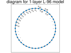
(a)

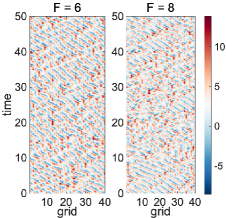
(b)

Figure 1: Illustration of the model structure and typical solutions of the one-layer L-96 system (18).

4.1.1 Explicit formulation and RBM approximation for the one-layer L-96 system

Here, we derive the explicit stochastic-statistical formulation for the one-layer L-96 system as an example to illustrate the main ideas and performance in the proposed strategy. In the L-96 system (18), randomness comes only from the initial condition and is amplified due to the internal instability. We seek the probability solution of the model state $p_{t}\left(\left\{u_{j}\right\}\right)$ starting from an initial distribution $p_{0}\left(\left\{u_{j}\right\}\right)$. Clearly, the L-96 system fits into the general framework (1). The periodic boundary condition implies the mean-fluctuation decomposition as in (4) by a Galerkin projection on the Fourier basis

$$u_{j}=\bar{u}_{j}+\frac{1}{J}\sum_{\left|k\right|\leq J/2}Z_{k}\left(t\right)e^{i2\pi k\frac{j}{J}},$$ (19)

where $\bar{u}_{j}=\left\langle u_{j}\right\rangle_{p_{t}}$ is the statistical mean and $\left\{Z_{k}\right\}$ are stochastic coefficients with $\left\langle Z_{k}\right\rangle_{p_{t}}=0$. Due to the constant forcing and damping terms, the resulting statistics in each moment of the solution state is translation invariant [28, 35]. It implies that the mean state, $\left\langle u_{j}\right\rangle_{p_{t}}=\bar{u}\left(t\right)$, is uniform; and the off-diagonal covariance entries are all vanishing, $R\left(t\right)=\left\langle\mathbf{Z}\mathbf{Z}^{*}\right\rangle_{p_{t}}=\mathrm{diag}\left\{r_{k}\left(t\right)\right\}$. Therefore, we can focus on the dynamical equations for the scalar mean $\bar{u}$ and variance $r_{k}$ of each Fourier mode together with the stochastic coefficients $Z_{k}$ to recover the entire statistics in this system.

The explicit full stochastic-statistical formulation (7) and the corresponding RBM model (8) for the L-96 system are listed in Appendix A.1. Due to the still relatively low dimension $J=40$ of the one-layer model, we apply the full RBM model in Algorithm 1 and test the random batch approximation for the full spectrum prediction involving a large number of highly unstable and energetic modes. We summarize several main features observed from using the RBM model on the one-layer L-96 system before showing the detailed discussions on the numerical results in the next section:

• The computational cost for the full model (B1) is $O\left(J+MJ^{2}+MJ^{2}\right)=O\left(J\left(1+2MJ\right)\right)$ where $J$ is the full dimension of the system and $M$ is the ensemble size to sufficiently sample the $J$-dimensional space. In the RBM approximation (B2), the computational cost is effectively reduced to $O\left(J\left(1+2M_{1}p\right)\right)$ with $p$ the batch size and $M_{1}\ll M$ is the sample size only required to sample the much smaller $p$-dimensional subspace in each batch. Especially, $p$ does not increase as the dimensional $J$ increases.

• The coupled formulation combining the variance equations for $r_{k}$ and stochastic equations for $Z_{k}$ with the relaxation factor $\epsilon$ is essential to reach the correct final equilibrium state. Using purely the stochastic equations for $Z_{k}$ is insufficient to recover the correct statistics when the sample size becomes small due to the strong model instability.

• The RBM approximation relies on the ergodicity and fast mixing of the small-scale modes. The L-96 system possesses a wide spectrum with large number of fluctuation modes showing distinctive time scales, making it a difficult test case for the RBM model. Still, accurate statistical prediction is achieved even with an extremely small batch size $p=2$. Prediction results can be further improved by reducing the time step size $\Delta t$.

4.1.2 Numerical tests on the one-layer L-96 model

In the numerical tests, we take two typical regimes of the L-96 system with $F=6$ (showing non-Gaussian statistics) and $F=8$ (showing near-Gaussian statistics). Th standard 4th-order Runge-Kutta scheme is adopted for the time integration with time step size $\Delta t=1\times 10^{-4}$. A large ensemble size $M=1\times 10^{5}$ is needed to capture the true model statistics accurately from the direct MC simulation. In the RBM prediction, different batch sizes $p=2,5,10$ are used to compute the high-order interactions compared with the full model using the entire $J=40$ modes. Therefore, only a very small sample size $M_{1}=100$ becomes sufficient, allowing for efficient computation.

First, we illustrate the inherent difficulty in running ensemble prediction for turbulent systems with instability. In the full model (B1), the variance equations for $r_{k}$ (as well as the stochastic equations for $Z_{k}$) are subject to internal instability due to the real part of the coupling coefficient $-\left(\gamma_{k}^{*}\bar{u}+1\right)$ representing interaction with the mean state $\bar{u}$. As illustrated in the left panel of Figure 2, positive growth rates are induced in a large number of modes as the system evolves in time. This indicates the crucial role of the combined third order moments $\left\langle Z_{m}Z_{n}^{*}Z_{k}^{*}\right\rangle$ acting as a balancing factor for these internally unstable modes. On the other hand, with insufficient sample size, large errors can be introduced to the empirical estimation of the higher-order feedback term. The inherent instability in the turbulent model formulation can be also seen in the zeroth mode equation (20). It shows that the equation is only marginally stable thus small errors in the ensemble estimation will lead to large errors.

In the practical simulation of the ensemble scheme, the internal instabilities will amplify the small errors and lead to disastrous result. The situation will become increasingly serious if we only want to use a small ensemble size. As a typical example shown on the right panel of Figure 2, we get the truth from the direct MC simulation of (18) with an extremely large ensemble size $M=1\times 10^{5}$. In comparison, we run the full model (B1) with several different values $\epsilon$ in the additional relaxation term $\epsilon^{-1}\left(\left\langle\left|Z_{k}\right|^{2}\right\rangle-r_{k}\right)$. It shows that even with this moderate dimension $J=40$ and very large ensemble size, the solution for the statistical mean and variance will diverge without the relaxation term $\epsilon=\infty$, while equilibrium consistency is guaranteed when smaller value of $\epsilon$ is added. It demonstrates the crucial role of the additional relaxation term to guarantee equilibrium converge. It also shows that the model is robust with consistent final statistics for a wide range of values of $\epsilon$ as long as it is not too large.

Remark.

As a simple example to illustrate the internal instability, the explicit equation for the zeroth mode $Z_{0}$ in the full model (B1) gives

$$\frac{\mathrm{d}Z_{0}}{\mathrm{d}t}=\frac{1}{J}\sum_{k}\gamma_{k}\left(\left|Z_{k}\right|^{2}-r_{k}\right)-Z_{0},$$ (20)

with $\gamma_{k}=\cos\frac{4\pi k}{J}-\cos\frac{2\pi k}{J}$. The consistent final equilibrium requires $\left\langle Z_{0}\right\rangle=\frac{1}{J}\sum_{k}\gamma_{k}\left(\left\langle\left|Z_{k}\right|^{2}\right\rangle-r_{k}\right)=0$, while instability will be introduced through errors due to the empirical average $\left\langle\left|Z_{k}\right|^{2}\right\rangle\sim r_{k}$. This will lead to inherent difficulty even with a very large sample size as shown in Figure 2.

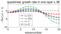
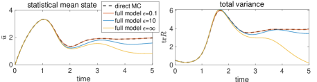
Figure 2: Effects of instability in the one-layer L-96 system with $F=6$. Left: quasilinear growth rate in each wavenumber $-\mathrm{Re}\left(\gamma_{k}^{*}\bar{u}+1\right)$ at several time instants; Right: direct solutions from the full model with different relaxation strengths $\epsilon$.

Next, we check the performance of the RBM prediction with different batch sizes. In the one-layer L96 model with $J=40$, we will focus on the fully resolved RBM model (B2) described in Algorithm 1. In Figure 3, the time-series of the mean $\bar{u}$ and total variance $\mathrm{tr}R=\sum r_{k}$ as well as the prediction for the detailed variance spectrum in each mode during the time evolution are plotted. Two batch sizes $p=5,2$ with $M_{1}=100$ samples from the RBM model prediction are compared with the truth from the direct MC simulation using $M=1\times 10^{5}$ samples for the full dimension $J=40$. Furthermore, we also test an extreme case with only $p=2$ modes (that is, only using one term in the high-order feedback for the strongly unstable dynamics) in each batch and a very small sample size $M_{1}=20$ in computing the statistics. It shows that all the RBM results accurately track the truth statistics with lines overlapping on each other while save a lot of computational cost using the extremely small ensemble. In particular, the L-96 system sets a challenging test model for the RBM model since it contains a wider spectrum of energetic modes containing large degrees of instabilities. Still, as shown in the energy spectra from the starting transient stage to the final equilibrium, the variances in all the modes are captured with high precision.

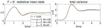
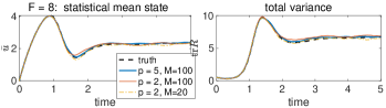
(a)

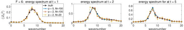
(b)

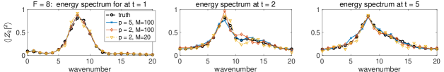
(c)

Figure 3: Time evolutions of the mean and total variance as well as the variance spectra from the RBM prediction with batch size $p=2,5$ and ensemble size $M_{1}=100,20$. Results from the two test regimes $F=6$ and $F=8$ are shown and the truth is recovered from a direct MC simulation with a large sample size $M=1\times 10^{5}$.

Then, another important goal of the RBM model is to accurately characterize the PDFs of the model states. This is especially important in application to uncertainty quantification and data assimilation, where an accurate estimate of PDFs using limited number of samples is crucial. In the RBM approach, the PDFs are captured by the empirical distribution (3) of the stochastic coefficients $Z_{k}$. Figure 4 first plots the 1D marginally PDFs in the leading Fourier modes $Z_{k}$ of the one-layer L-96 system in the two test regimes. It shows that the $F=6$ regime generates stronger non-Gaussian PDFs while the $F=8$ regime is closer to Gaussian but still contains non-negligible non-Gaussian features. Usually, a very large ensemble is essential to capture such non-Gaussian statistics in the direct MC approach. Using the efficient RBM approximation, the shapes PDFs including the skewed and sub-Gaussian structures are accurately characterized using a very small ensemble size $M_{1}=100$. As a more precise calibration of the prediction of PDFs, we plot the 2D joint PDFs between the most important modes in Figure 5. The non-Gaussian structures can be observed more clearly in the joint distributions. The outliers in the sampled PDFs play an important role to characterize the occurrence of extreme events and have crucial impact in many practical applications with limited samples. The RBM model successfully captures the joint PDFs especially recovers the representative non-Gaussian shapes in the outlier regions though using only a very small number of samples.

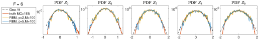
(a)

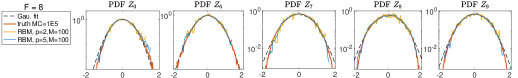
(b)

Figure 4: 1D marginal PDFs of the stochastic coefficients $Z_{k}$ in the two test regimes $F=6,8$ of the one-layer L-96 system. The RBM predictions with sample size $M_{1}=100$ are compared with the truth from direct MC simulation with $M=1\times 10^{5}$. The Gaussian fits of the PDFs with the same mean and variance are also plotted in dashed lines.

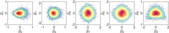
(a) MC $F=6$

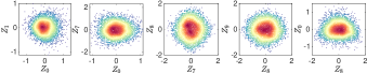
(b) MC $F=8$

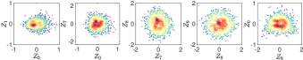
(c) RBM $F=6$

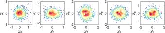
(d) RBM $F=8$

Figure 5: 2D joint PDFs of the leading modes in the two test regimes $F=6,8$ of the one-layer L-96 system. The RBM predictions with sample size $M_{1}=100$ are compared with the truth from direct MC simulation with $M=1\times 10^{5}$.

Finally, we provide a quantitative quantification of the model errors of the RBM prediction with different batch sizes $p$. In particular, one of the central quantities to estimate in the RBM is the second moments, thus we consider the time-averaged errors in the variance prediction $\left\|R_{\mathrm{m}}-R_{\mathrm{t}}\right\|=\frac{1}{N}\sum_{s=1}^{N}\sum_{k}\left|r_{\mathrm{m},k}\left(t_{s}\right)-r_{\mathrm{t},k}\left(t_{s}\right)\right|$ where $R_{\mathrm{m}}$ is the RBM prediction and $R_{\mathrm{t}}$ is the truth. Figure 6 plots the errors with the batch sizes $p=2,5,10$ and sample size $M_{1}=500$. We use a relatively larger sample size to reduce the fluctuation errors from the small ensemble. The convergence of RBM estimates depends on the average on the random batches (thus equivalently on time average of the fast mixing modes), therefore the errors grow as the time step size $\Delta t$ increases. A smaller batch size will lead to larger errors due to the fewer high-order terms explicitly modeled at each time updating step. When the time step decreases to smaller values, the major source of errors is taken over by the fluctuation errors from the small ensemble size, so the decay of the errors starts to slow down. Also the larger batch size $p=10$ shows a slower decay rate since it needs to sample a relatively larger dimensional batch subspace in computing the nonlinear coupling terms. Overall, the error plot shows that the RBM model remains uniformly high prediction skill in accurately recovering the key statistics with a much lower affordable computational cost. It also implies that it is a good strategy to improve the prediction accuracy by taking a smaller time step $\Delta t$ without increasing much of the computational cost.

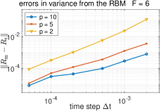
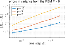
Figure 6: Errors in the total variance from the RBM prediction with different batch sizes $p=2,5,10$ in the two test regimes $F=6,8$ of the one-layer L-96 system.

4.2 The two-layer L-96 system

In the second test model, we examine the model effectiveness in handling truly high-dimensional systems with multiscale structures by considering the more complicate two-layer L-96 system. As a further generalization of the original one-layer system, the two-layer L-96 system [1, 46] introduces an additional second layer state $v_{i},i=1,\cdots,JL$ to the first layer state $u_{j},j=1,\cdots,J$ such that

$$\frac{du_{j}}{dt} =\left(u_{j+1}-u_{j-2}\right)u_{j-1}-u_{j}+F-\frac{hc}{b}\sum_{i=L\left(j-1\right)+1}^{jL}v_{i},$$ (21)

$$\frac{\mathrm{d}v_{i}}{\mathrm{d}t} =-cb\left(v_{i+2}-v_{i-1}\right)v_{i+1}-cv_{i}+\frac{hc}{b}u_{\left[\frac{i-1}{L}\right]+1},$$

both with periodic boundary conditions, $u_{j+J}=u_{j}$ and $v_{i+JL}=v_{i}$. Above, $u$ is usually referred to as the large-scale slow variables and $v$ as the small-scale fast variables. On the right hand sides of (21), the double layer states follow the same energy-conserving nonlinear self-coupling structure as well as uniform linear damping effect as in the one-layer case. The two states of different scales are then coupled through three additional model parameters, $c,b,h$: $c$ signifies the time-scale separation; $b$ controls the ratio between the amplitudes of two layer states $u_{j}$ and $v_{i}$; and $h$ characterizes the coupling strength between the two states. We illustrate the coupling structure of the two-layer system in the diagram of Figure 7. In particular, the second layer states $v_{i}$ for $i=1,\cdots,JL$ are locally coupled with one corresponding first layer state $u_{j}$ with the index $j=\left[\frac{i-1}{L}\right]+1$ (where $\left[a\right]$ takes the integer part of $a$), and are globally linked with each other by the nonlinear self-interactions. Inversely, each first layer state $u_{j}$ receives the combined feedback from a sequence of $L$ second layer states $v_{i}$, $i=L\left(j-1\right)+1,\cdots,jL$. This leads to a fully coupled high-dimensional system including the two-level states $\left\{u_{j},v_{i}\right\}$ with a total of $J\left(L+1\right)$ state variables. The multiscale structure of the dynamical solution is demonstrated by a typical time-series of the large and small scale processes. It is clear to observe the distinctive time and spatial scales and close correlation between the two scales.

The model parameters used in the numerical tests are listed in Table 1 taken the standard model setup as in [46, 1, 15]. Especially, we consider two typical parameter regimes with a mild time-scale separation $c=4$ and a strong time-scale separation $c=10$. Again, the two-layer L-96 system displays strong internal instability containing a large number of unstable modes with positive growth rates as shown in Figure 7. To recover the true model statistics with sufficient accuracy, we need to take a small time step $\Delta t=1\times 10^{-4}$ in order to completely resolve the extremely fast time scales in the second layer variables $v_{i}$. A forth-order Runge-Kutta scheme is adopted for the time integration in both the direct MC simulation and the RBM approaches. A very large ensemble size $M=5\times 10^{5}$ is required considering the very high-dimension $d=J\left(L+1\right)=264$ of the system. In contrast, it is sufficient to only use $M_{1}=O\left(100\right)$ samples in both the full and reduced-order RBM approaches.

$J$	$L$	$F$	$c$	$b$	$h$		$\Delta t$	$M$	$M_{1}$
8	32	20	4, 10	10	1		$1\times 10^{-4}$	$5\times 10^{5}$	500, 100

Table 1: Model parameters used for the two-layer L-96 model (21)

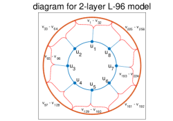
(a)

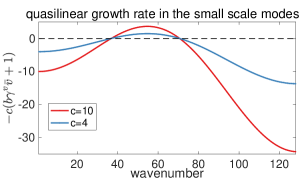
(b)

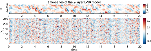
(c)

Figure 7: Illustration of the two-layer L-96 system with large-scale size $J=8$ and small-scale size $JL=256$. Upper: diagram for the model structure and growth rates in the small-scale modes; Lower: a typical time-series solution for the large and small scale states with $c=4,b=10,h=1$.

4.2.1 Stochastic-statistical formulation for the two-layer L-96 system

Similar to the one-layer L-96 system, we can project the large and small scale states to the Fourier modes due to the periodic boundary condition for both $u_{j}$ and $v_{i}$ as

$$u_{j}=\bar{u}+\frac{1}{J}\sum_{\left|k\right|\leq J/2}Z_{k}\left(t\right)e^{i2\pi k\frac{j}{J}},\quad v_{i}=\bar{v}+\frac{1}{JL}\sum_{\left|l\right|\leq JL/2}Y_{l}\left(t\right)e^{i2\pi l\frac{i}{JL}},$$ (22)

where $Z_{k}$ and $Y_{l}$ are the stochastic coefficients for the large and small scale states correspondingly. The two-layer L-96 system (21) also accepts the general system structure (1). Using the translation invariance in both large and small scales, the statistical prediction aims to recover the homogeneous mean states $\bar{u}\equiv\left\langle u_{j}\right\rangle_{p_{t}}$ and $\bar{v}\equiv\left\langle v_{i}\right\rangle_{p_{t}}$, and the variances in large and small scale modes $r_{k}^{u}=\left\langle\left|Z_{k}\right|^{2}\right\rangle_{p_{t}},r_{l}^{v}=\left\langle\left|Y_{l}\right|^{2}\right\rangle_{p_{t}}$ according to the model probability measure $p_{t}$. The detailed equations involving various linear and nonlinear coupling effects between different scales become very complicated. We list the explicit mean and covariance equations involving complicated higher-order coupling terms across the scales in Appendix A.2.

The most important ideas concerning the RBM approximation of the two-layer L96 system (21) can be illustrated in the stochastic equations for the large and small scale fluctuation modes

$$\frac{\mathrm{d}Z_{k}}{\mathrm{d}t} =\frac{1}{J}\sum_{m-n=k}\left(Z_{m}Z_{n}^{*}-r_{m}^{u}\delta_{mn}\right)\gamma_{mn}^{u}-d_{u}Z_{k}-\frac{1}{L}\sum_{s=-L/2+1}^{L/2}\lambda_{k+sJ}^{*}Y_{k+sJ},$$ (23)

$$\frac{\mathrm{d}Y_{l}}{\mathrm{d}t} =\frac{1}{JL}\sum_{p-q=l}\left(Y_{p}Y_{q}^{*}-r_{p}^{v}\delta_{pq}\right)\gamma_{pq}^{v}-d_{v}Y_{l}+\lambda_{l}Z_{\mathrm{mod}\left(l,J\right)}.$$

Above, we have the coupling coefficients $\gamma_{mn}^{u}=e^{2\pi i\frac{m+n}{J}}-e^{-2\pi i\frac{2m-n}{J}}$, $\gamma_{pq}^{v}=cb\left(e^{-2\pi i\frac{p+q}{JL}}-e^{2\pi i\frac{2p-q}{JL}}\right)$, $\lambda_{l}=\frac{hc}{b}\frac{1-e^{-2\pi i\frac{l}{J}}}{1-e^{-2\pi i\frac{l}{JL}}}$, and the quasilinear operator for interaction with the mean states, $d_{u}=1+\gamma_{k}^{u*}\bar{u}$, $d_{v}=c\left(1+b\gamma_{l}^{v*}\bar{v}\right)$ (see the detailed model parameters in (B4)). Notice that in the large-scale modes, the indices in the summation for nonlinear coupling go through all the wavenumbers, $\left|m\right|\leq J/2$, while in the small-scale modes the indices for nonlinear coupling include all the small-scale wavenumbers, $\left|p\right|\leq JL/2$. This leads to an extremely high computational overload considering the high dimension of the small-scale modes. Finally, the large and small scale modes are coupled through the last linear terms. Especially, the small-scale modes $Y_{k+sJ},\left|s\right|\leq L/2$ give a combined feedback to the large-scale mode $Z_{k}$, while each $Z_{k}$ is acting on a sequence of small-scale modes $Y_{k+sJ}$. It is realized that in (23) the most computational demanding part comes from the summation terms going through all the wavenumbers representing both linear and nonlinear coupling between scales.

Next, we present the performance of the RBM models on the two-layer L-96 with genuinely high dimensional and multscale scale processes. In particular, we first consider the full RBM model in Algorithm 1, then further reduce the computational cost by applying the reduced-order RBM model in Algorithm 2 exploiting the large number of fast-mixing small-scale modes.

4.2.2 Numerical results for the full RBM model

First, we consider the full RBM approximation, that is, to introduce random batch decomposition in both the large and small scale stochastic modes $\left\{Z_{k}^{\left(i\right)},Y_{l}^{\left(i\right)}\right\}$, while still run independent samples for ensemble simulation of the entire stochastic equations during each time updating interval. This leads to the full RBM model for the stochastic coefficients of the two-layer L-96 system following the general formulation (8)

$$\frac{\mathrm{d}Z_{k}^{\left(i\right)}}{\mathrm{d}t} =c_{p}\sum_{m\in\mathcal{I}_{k}^{s}}\left(Z_{m}^{\left(i\right)}Z_{m-k}^{\left(i\right)*}-r_{m}^{u}\delta_{m,m-k}\right)\gamma_{m,m-k}^{u}-d_{u}Z_{k}^{\left(i\right)}-c_{L}\sum_{k+sJ\in\mathcal{J}_{l}^{s}}\lambda_{k+sJ}^{*}Y_{k+sJ}^{\left(i\right)},$$ (24)

$$\frac{\mathrm{d}Y_{l}^{\left(i\right)}}{\mathrm{d}t} =c_{q}\sum_{p\in\mathcal{J}_{l}^{s}}\left(Y_{p}^{\left(i\right)}Y_{p-l}^{\left(i\right)*}-r_{p}^{v}\delta_{p,p-l}\right)\gamma_{p,p-l}^{v}-d_{v}Y_{l}^{\left(i\right)}+\lambda_{l}Z_{\mathrm{mod}\left(l,J\right)}^{\left(i\right)},$$

with independent samples $i=1,\cdots,M_{1}$. In the RBM approximation at each time updating step $t=t_{s}$, we choose the batches $\cup_{k}\mathcal{I}_{k}^{s}=\left\{k:\left|k\right|\leq\frac{J}{2}\right\}$ with batch size $p=\left|\mathcal{I}_{k}^{s}\right|$ for the large-scale modes $Z_{k}$, and batches $\cup_{l}\mathcal{J}_{l}^{s}=\left\{l:\left|l\right|\leq\frac{JL}{2}\right\}$ with $q=\left|\mathcal{J}_{l}^{s}\right|$ for the small-scale modes $Y_{l}$. Then the original summation terms taking over the entire spectrum space are reduced to the summation for modes restricted inside one batch of very small size $\left(p,q\right)$ (with the pair elements corresponding to large and small scale batch sizes). The new normalization factors can be found as $c_{p}=\frac{1}{J}\frac{J-1}{p-1}$, $c_{q}=\frac{1}{JL}\frac{JL-1}{q-1}$, and $c_{L}=\frac{1}{L}\frac{L-1}{q-1}$ following the same principle as the one-layer case. The corresponding RBM equations for the associated covariance equations can be derived accordingly. We list the explicit equations in Appendix A.2. In this way, the computational cost for the nonlinear coupling terms, particularly the small scales with a large number of modes, are greatly saved by constraining the high-order interactions only inside the very small batch. This leads to the effective reduction in computational cost to $O\left(M_{1}J\left(p+Lq\right)\right)$ in solving the stochastic equations compared to the original cost $O\left(MJ^{2}\left(1+L^{2}\right)\right)$ in the direct MC approach in computing the full ensemble of size $M\gg M_{1}$.

In the numerical test of the full RBM model, we take the model parameters for the standard regime $c=10,b=10,h=1,F=20$ and $J=8,L=32$. The resulting coupled large and small-scale processes form a very high total dimension $d=J\left(L+1\right)=264$. In particular, the small-scale variable $v_{i}$ has a much faster time scale and the large scale state $u_{j}$. This leads to a more challenging multiscale problem since we have to resolve the large number of small scale modes even that we are only interested in the large-scale state. In order to get accurate statistical prediction resolving all the multiscale features, we use a very large ensemble size $M=5\times 10^{5}$ for the direct MC simulation to accurate recover the true reference solution. In the RBM model, three different batch pairs $\left(p,q\right)=\left(4,16\right),\left(4,8\right),\left(2,4\right)$ are tested in contrast to the total number of modes $\left(J,JL\right)=\left(8,256\right)$. A much smaller ensemble size $M_{1}=500$ is used and this is made possible by sampling only the $q$-dimensional subspace instead of the $JL$-dimensional full space of the small scales.

In Figure 8, we first show the RBM model prediction for the mean $\bar{u},\bar{v}$ and average total variance $\sum r_{k}^{u}/J,\sum r_{l}^{v}/JL$ with three different batch sizes, as well as the pointwise errors in mean and total varianc at each time step. It shows accurate recovery of the key statistics in both the mean and variance, and in both the starting transient stage and final equilibrium. The high accuracy is maintained with almost indistinguishable results as we reduce the batch sizes $\left(p,q\right)$. Relatively larger errors are observed in the starting transient stage when a small batch size is applied. Notice that significant computational reduction is achieved where the smallest batch size refers using only $q=4$ nonlinear coupling terms for each $Y_{l}$ out of the total $JL=256$ terms. In addition, the detailed model prediction for the variance spectra in each large and small scale modes is shown in Figure 9. A wide range of the small-scale modes with high wavenumbers are excited due to the instability in small scales, as illustrate in Figure 7. This presents a highly challenging scenario as we only resolve a very small batch of modes for the nonlinear coupling term to stabilize the large number of unstable modes. Again, the energy spectrum is recovered exactly with uniformly high skill using the three extremely small batch sizes. This highlights the robust skill in the RBM model to achieve computational efficiency and maintain high prediction accuracy at the same time.

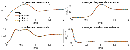
(a)

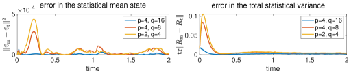
(b)

Figure 8: Prediction of the mean and averaged variance in both large and small scale modes from full RBM model with different batch sizes $\left(p,q\right)$ compared with the full MC model with $JL=256$ modes in small scales and sample size $M=5\times 10^{5}$. $M_{1}=500$ samples are used for all the RBM models. The trajectory errors in the mean and variance are also compared.

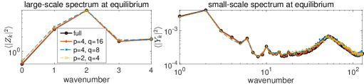
Figure 9: Prediction of the variance spectra for large and small scale modes in full RBM model with different batch sizes $\left(p,q\right)$ compared with the full MC model with $JL=256$ modes in small scales and sample size $M=5\times 10^{5}$.

Next, we proceed to check the ability of the RBM model to capture the PDFs of the dominant modes. Figure 10 shows the marginal PDFs of the leading stochastic modes in both large and small scales. In this case of the two-layer L-96 system, even stronger non-Gaussian statistics are displayed with highly skewed and fat-tailed PDFs. Accurate characterization of such non-Gaussian PDFs becomes even more critical issue in statistical prediction of such high-dimensional systems. Usually, the small number of samples tend to concentrate near the central part of the PDF and miss the crucial extreme events featuring the edge regions of the large phase space. Using the RBM model with a very small ensemble size, the strongly non-Gaussian PDFs are successfully captured confirming the very high skill of the RBM approach in recovering the true model statistics not only in the leading moments but also in the more challenging higher-order statistics. In addition, we also compare the joint PDFs in the predicted leading modes in Figure 11. The non-Gaussian structures become more pronounced in the 2D distributions, revealing bimodal PDFs as already indicated in the marginal PDFs. The RBM predictions maintain very accurate in recover the highly non-Gaussian statistics despite using a very small ensemble size.

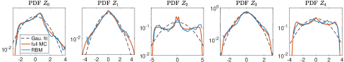
(a) large-scale modes

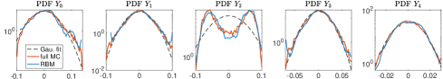
(b) small-scale modes

Figure 10: 1D marginal PDFs of the leading large and small scale stochastic modes $Z_{k},Y_{l}$ of the two-layer L-96 system. The RBM predictions are compared with the truth from direct MC simulation. The Gaussian fits of the PDFs with the same mean and variance are also plotted in dashed lines.

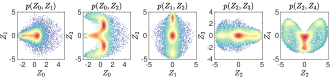
(a) MC large scale $Z_{k}$

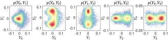
(b) MC small scale $Y_{l}$

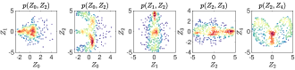
(c) RBM large scale $Z_{k}$

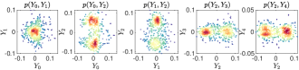
(d) RBM small scale $Y_{l}$

Figure 11: 2D joint PDFs of the leading large and small scale stochastic modes $Z_{k},Y_{l}$ of the two-layer L-96 system. The RBM predictions are compared with the truth from direct MC simulation.

Finally, we provide a quantitative comparison of the RBM model prediction errors as the key model parameters change. In Figure 12, we show the averaged errors in the total variance $\left\|R_{\mathrm{m}}-R_{\mathrm{t}}\right\|=\frac{1}{N}\sum_{s=1}^{N}\sum_{k}\left|r_{\mathrm{m},k}\left(t_{s}\right)-r_{\mathrm{t},k}\left(t_{s}\right)\right|$ and the mean $\left\|\bar{v}_{\mathrm{m}}-\bar{v}_{\mathrm{t}}\right\|^{2}=\frac{1}{N}\sum_{s=1}^{N}\left|\bar{v}_{\mathrm{m}}\left(t_{s}\right)-\bar{v}_{\mathrm{t}}\left(t_{s}\right)\right|^{2}$ according to the time integration step $\Delta t=t_{s+1}-t_{s}$ with two batch sizes $\left(p,q\right)=\left(4,16\right),\left(4,8\right)$ and two ensemble sizes $M_{1}=500,100$. The errors grow with larger time step size and with smaller ensemble and batch sizes agreeing with the intuition. Among the range of large to moderate time step sizes, reducing the time step can effectively improve the prediction accuracy since it is corresponding to more frequent resampling (thus more equivalent samples in the time average) in the RBM approximation. With very small time step size though, the error will saturate because the small ensemble size will account for the major error in the statistical estimates. It also implies that it might be useful to use a smaller batch size $q$ with a relatively larger ensemble to achieve accurate prediction with minimum computational cost.

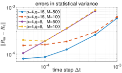
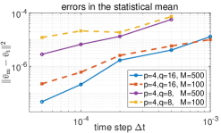
Figure 12: Errors in the statistical mean and total variance from the RBM prediction with different batch and ensemble sizes for the two-layer L-96 system.

4.2.3 Numerical results for the reduced-order RBM model

Next, we consider a further reduction of computation cost by applying the reduced-order RBM model as described in Algorithm 2. In the reduced RBM model, we still keep the statistical mean and covariance equations (B3) and (B5) the same as the full RBM model case. In the two-layer L-96 system, most of the computational cost comes from the ensemble simulation for the stochastic coefficients in (23) for the wide range of small-scale modes $Y_{l}$. In most situations, we are mostly interested in the statistics in the main large-scale modes $Z_{k}$ while the small-scale modes give crucial combined feedback to affect the large-scale state, thus their contributions cannot be simply ignored. The unstable growth (shown in Figure 7) and excited small scales in equilibrium energy spectrum (in Figure 9) emphasize the non-negligible role of these small-scale modes. This sets the inherent obstacle in developing effective reduced-order models for multiscale systems.

To enable further computational reduction for the small-scale modes, following the idea in (10) we group the ensemble members in the large scale modes $\mathbf{Z}^{\left(i\right)},i=1,\cdots,M_{1}$ with one single small-scale state $\mathbf{Y}$. In applying the RBM approximation, the same partition $\mathcal{I}_{k}^{s}$ is applied to the small number of large-scale modes. The model reduction strategy is applied to the expensive small-scale equations. The large number of small-scale modes are then divided into the batches $\mathcal{J}_{i}^{s}$, satisfying $\cup_{i=1}^{M_{1}}\mathcal{J}_{i}^{s}=\left\{l:\left|l\right|\leq JL/2\right\}$. According to the modes in the batches, the full system is decomposed into much smaller subsystems with one large-scale sample $\mathbf{Z}^{\left(i\right)}$ together with a portion of the small-scale modes $Y_{l},l\in\mathcal{J}_{i}^{s}$. The model reduction is made possible by the very large number of fast-mixing small-scale modes. This leads to the coupled equations for the stochastic coefficients in subsets $\left\{\mathbf{Z}^{\left(i\right)},Y_{l}\right\}_{l\in\mathcal{J}_{i}^{s}}$ during the time interval $t\in\left(t_{s},t_{s+1}\right]$

$$\frac{\mathrm{d}Z_{k}^{\left(i\right)}}{\mathrm{d}t}= c_{p}\sum_{m\in\mathcal{I}_{k}^{s}}\left(Z_{m}^{\left(i\right)}Z_{m-k}^{\left(i\right)*}-r_{m}^{u}\delta_{m,m-k}\right)\gamma_{m,m-k}^{u}-d_{u}Z_{k}^{\left(i\right)}-c_{L}\sum_{k+sJ\in\mathcal{J}_{i}^{s}}\tilde{\lambda}_{k+sJ}^{*}Y_{k+sJ},$$ (25)

$$\frac{\mathrm{d}Y_{l}}{\mathrm{d}t}= c_{q}\sum_{p\in\mathcal{J}_{i}^{n}}\left(Y_{p}Y_{p-l}^{*}-r_{p}^{v}\delta_{p,p-l}\right)\gamma_{p,p-l}^{v}-d_{v}Y_{l}+\tilde{\lambda}_{l}Z_{\mathrm{mod}\left(l,J\right)}^{\left(i\right)},\qquad l\in\mathcal{J}_{i}^{n}.$$

Above, the ensemble is used only to sample the low-dimensional large-scale state $\mathbf{Z}^{\left(i\right)}\in\mathbb{R}^{J}$, while only a small portion of small-scale modes $\left\{Y_{l}\right\}_{l\in\mathcal{I}_{i}}$ are grouped with the $i$-th sample $\mathbf{Z}^{\left(i\right)}$ together for the time update at $t=t_{s}$. The union of all the randomly sampled groups form the entire spectrum of small-scale modes. In this way, we no longer need to run a very large ensemble for the small scales $Y_{l}$ by exploiting its wide spectrum of modes acting at different large-scale samples. Notice that the samples $\mathbf{Z}^{\left(i\right)}$ will no longer stay independent and will be linked by the small-scale modes through the random batches. Still, the important correlations between the small and large scale modes are maintained through this splitting of small-scale modes.

Remark.

In practice, we may still want to run a small number of small-scale modes $\mathbf{Y}^{\left(j\right)},j=1,\cdots,M_{2}$. This is equivalent to introduce an ensemble of size $M_{2}$ to the above block model (25), so that the model parameters have the relation $\kappa=\frac{M_{1}}{M_{2}}=\frac{JL}{2q}$. For consistent statistics, the large and small scale coupling coefficient needs to be updated as $\tilde{\lambda}_{l}=\sqrt{\kappa}\lambda_{l}$. This leads to the computational reduction from $O\left(M_{1}J\left(p+Lq\right)\right)$ in the full RBM model to $O\left(M_{1}Jp+M_{2}JLq\right)=O\left(M_{1}\left(q^{2}+pJ\right)\right)$ which is only dependent on the dimension $J$ of the large-scale state and independent of the small scale dimension $JL$.

In the numerical test of the reduced-order model, we consider the parameter regime of the two-layer L-96 system with $c=4,b=10,h=1,F=20$. This regime gives a weaker scale separation between the large and small scales thus sets a more important role for the small-scale processes with a non-negligible contribution to the large-scale modes. We fix the batch size as $\left(p,q\right)=\left(4,32\right)$. The relatively large batch size $q=32$ (compared with the full dimension $JL=256$) is used to ensure a larger allowed sample size $M_{2}=\frac{2qM_{1}}{JL}$ for the small-scale modes. We pick a moderate sample size $M_{1}=500$ to sample the large-scale mode of dimension $J$ and the large number of small-scale modes only requires a small sample size $M_{2}=125$. Another extreme sample size $M_{1}=100,M_{2}=25$ is also tested. The reduced-order model enables even more efficient computation compared with the very high dimension of the full system $d=J\left(L+1\right)=264$.

We show the prediction results in the reduced-order RBM model in Figure 13. It can be seen that the reduced model maintains the high skill to capture the leading statistics in both the large and small scale states while save additional computational cost by avoiding running the large ensemble simulation. The pointwise errors in mean and variance further confirm the accurate statistical prediction even with a small and reduced sample size. Accordingly, we show the detailed prediction of the energy spectra at several time instants in both large and small scale modes in Figure 14. In the case of reduced-order model due to the very small ensemble size, it is expected the small-scale modes will become very noisy and have larger fluctuation errors especially for the large wavenumber modes. Still, the reduced-order RBM model successfully captures the structure of spectra in both large and small scales. These encouraging results suggest further applications of the RBM models to more practical and realistic systems exhibiting stronger multiscale coupling and a very wide spectrum covering a large number of scales.

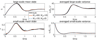
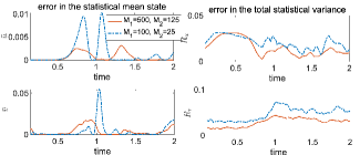
Figure 13: Prediction of the mean and variances in the reduced-order RBM model with batch size $\left(p,q\right)=\left(4,32\right)$ and sample size $(M_{1},M_{2})=(500,125),(100,25)$ with for $M_{1}$ samples for large-scale state and $M_{2}$ for small-scale state. The time evolutions of the errors in mean and variance are also compared.

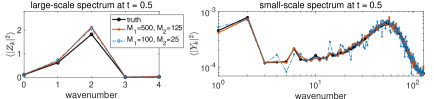
(a)

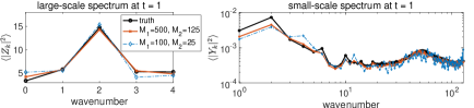
(b)

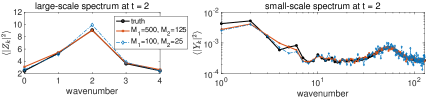
(c)

Figure 14: Reduced-order RBM model prediction of the variance spectra in both large and small scale modes at several time instants $t=0.5,1,2$.

5 Summary

We present a systematic closure modeling framework that enables efficient ensemble prediction of leading-order statistics and non-Gaussian PDFs in complex turbulent systems, which are characterized by strong internal instability and interactions of coupled spatio-temporal scales. A general stochastic-statistical formulation is established derived from a generic multiscale nonlinear system, capable of modeling a wide range of complex phenomena observed in natural and engineering systems. A mean and fluctuation decomposition of the original model state is introduced to deal with the irreducible dynamics in the high-dimensional equations. The fluctuation modes, which capture large uncertainty in multiscale modes, are modeled using stochastic equations that depend on the mean state and covariance of fluctuation modes. The leading-order statistical equations for the mean and covariance incorporate higher-order moment feedback from different scales. A precise high-order closure is introduced using empirical average of the ensemble prediction of the stochastic equation solution, which explicitly captures detailed multiscale interactions. The coupling between stochastic and statistical equations is further reinforced by a relaxation term for statistical consistency. This approach effectively balances the strong internal instability often encountered in turbulent systems, mitigating the inherent problem of numerical divergence in the statistical solution. The model achieves high skill in capturing non-Gaussian statistics and extreme outliers by explicitly resolving crucial higher-order moments instead of relying on insufficient low-order parameterizations. The stochastic-statistical formulation offers a flexible approach for recovering essential model statistics, making it applicable to a wide range of problems in uncertainty quantification and data assimilation [42, 39, 3].

To enable efficient computation using a small ensemble size for the stochastic equation and limit the number of high-order nonlinear coupling terms during each time update, we generalize the idea in RBM approximation for mean-fluctuation equations [37]. The approach decomposes the wide spectrum involving large number of multiscale modes into small random batches. A much smaller ensemble size is made possible by just sampling the nonlinear coupling terms involving modes in a low-dimensional subspace inside one batch. Simutaneously, the contribution from all the other modes is fully modeled by resampling the batches at each time step, exploiting the ergodicity of the stochastic modes. Consequently, high prediction accuracy concerning all high-order feedbacks is achieved. For systems with exceptionally high dimensionality, a model reduction strategy is proposed to further reduce the computational cost by linking the large number of small-scale fluctuation modes to the ensemble samples of large-scale state. The resulting algorithms are straightforward to implement and are well-suited for a wide range of multiscale turbulent systems. We evaluate the performance of the proposed RBM models using the representative one-layer and two-layer L-96 systems, which exhibit strong multiscale coupling and a wide spectrum of energetic unstable modes. The models demonstrate uniform high prediction skill for the leading order mean and variance, and more notably, capture the highly non-Gaussian PDFs and extreme events using a very small ensemble. As a result, the computational cost is reduced to an affordable level for genuinely high dimensional systems. In future research directions, we aim to develop a complete theory to analyze the general stochastic-statistical modeling framework building upon the preliminary estimates presented in this paper. The promising results also suggest potential applications to more realistic high-dimensional systems. The reduced-order RBM model shows potential in overcoming the curse of dimensionality and providing an effective tool for a wide range of practical problems related to prediction and data assimilation.

Data Availability

The data that support the findings of this study are available from the corresponding author upon reasonable request.

Appendix A Proof of theorems in Section 3.3

Proof of Theorem 1.

Define the following functions according to solutions to (11a) and (11b)

$$\tilde{w}\left(\mathbf{x},t\right)= \frac{1}{K}\sum_{k=1}^{K}\mathbb{E}_{\mathbf{x}}\varphi\left(\tilde{Z}_{k}\left(t\right)\right),$$ (A1)

$$w\left(\mathbf{x},t\right)= \frac{1}{K}\sum_{k=1}^{K}\mathbb{E}_{\mathbf{x}}\varphi\left(Z_{k}\left(t\right)\right),$$

with the test function $\varphi\in C_{b}^{2}$ and initial state $\mathbf{Z}\left(0\right)=\tilde{\mathbf{Z}}\left(0\right)=\mathbf{x}\in\mathbb{R}^{K}$. The the functions (A1) defined in the time interval $t\in\left(t_{s},t_{s+1}\right]$ are governed by the backward Kolmogorov equation [45] as

$$\partial_{t}\tilde{w}=\tilde{\mathcal{L}}_{\mathcal{I}^{s}}\tilde{w} =\sum_{k=1}^{K}\left[\sum_{m,n}I_{k}^{s}\left(m\right)\tilde{L}_{v,km}\left(\bar{u}\right)x_{m}+I_{k}^{s}\left(m\right)I_{k}^{s}\left(n\right)\tilde{\gamma}_{mnk}\left(x_{m}x_{n}-R_{mn}\right)\right]\cdot\partial_{x_{k}}\tilde{w}+\frac{1}{2}\sum_{k=1}^{K}\sigma_{k}^{2}\partial_{x_{k}}^{2}\tilde{w},$$ (A2)

$$\partial_{t}w=\mathcal{L}w =\sum_{k=1}^{K}\left[\sum_{m,n}L_{v,km}\left(\bar{u}\right)x_{m}+\gamma_{mnk}\left(x_{m}x_{n}-R_{mn}\right)\right]\cdot\partial_{x_{k}}w+\frac{1}{2}\sum_{k=1}^{K}\sigma_{k}^{2}\partial_{x_{k}}^{2}w.$$

Above in (A2), the backward equation for the RBM model $\tilde{w}$ is subject to the additional randomness due to the partition $\mathcal{I}^{s}=\left\{\mathcal{I}_{k}^{s}\right\}$ during the time updating interval. We introduce the index function defined in time $t\in\left(t_{s},t_{s+1}\right]$

$$I_{k}^{s}\left(m\right)=\begin{cases}1,&\mathrm{if}\>m\in\mathcal{I}_{k}^{s},\\ 0,&\mathrm{otherwise.}\end{cases}$$

Notice that the functions $I_{k}^{s}$ is kept constant during each time interval $\left(t_{s},t_{s+1}\right]$ and will change values subject to the resampling of the random batches. According to the conclusion in [37], we have the expectation of the partition functions by counting the ordered combinations of the random batches

$$\mathbb{E}I_{k}^{s}\left(m\right)=\frac{p}{K},\quad\mathbb{E}I_{k}^{s}\left(m\right)I_{k}^{s}\left(n\right)=\frac{p}{K}\frac{p-1}{K-1}.$$

This leads to the consistent condition on the expectation with the partition using the proper choice of the coupling coefficients

$$\mathbb{E}^{\mathcal{I}^{s}}\tilde{\mathcal{L}}_{\mathcal{I}^{s}}=\mathcal{L}.$$

Using the semigroup operator $\tilde{\mathcal{S}}$ acting on the function $w\left(\mathbf{x},t_{s}\right)$ and the above identity, we have

$$\tilde{\mathcal{S}}w\left(\mathbf{x},t_{s}\right)-w\left(\mathbf{x},t_{s+1}\right) =\mathbb{E}^{\mathcal{I}^{s}}e^{\Delta t\tilde{\mathcal{L}}_{\mathcal{I}^{s}}}w\left(\mathbf{x},t_{s}\right)-w\left(\mathbf{x},t_{s+1}\right)$$

$$=\int_{0}^{\Delta t}\left(\Delta t-\tau\right)\left[\mathbb{E}^{\mathcal{I}^{s}}\left(\tilde{\mathcal{L}}_{\mathcal{I}^{s}}\right)^{2}e^{\tau\tilde{\mathcal{L}}_{\mathcal{I}^{s}}}-\mathcal{L}^{2}e^{\tau\mathcal{L}}\right]w\left(\mathbf{x},t_{s}\right)\mathrm{d}\tau.$$

By the assumptions (12), the residual terms on the last equality are uniformly bounded

$$\left\|\left(\tilde{\mathcal{L}}_{\mathcal{I}^{s}}\right)^{2}e^{\tau\tilde{\mathcal{L}}_{\mathcal{I}^{s}}}w\left(\cdot,t\right)\right\|_{\infty}<C,\quad\left\|\mathcal{L}^{2}e^{\tau\mathcal{L}}w\left(\cdot,t\right)\right\|_{\infty}<C.$$

Therefore, the one-step error for between the RBM solution $\tilde{\mathcal{S}}w\left(\mathbf{x},t_{s}\right)$ and the full model $w\left(\mathbf{x},t_{s+1}\right)$ can be estimated as

$$\left\|\tilde{\mathcal{S}}w\left(\cdot,t_{s}\right)-w\left(\cdot,t_{s+1}\right)\right\|_{\infty}\leq C\Delta t^{2}.$$

Finally, by applying $\tilde{\mathcal{S}}$ on the initial function $w\left(\mathbf{x},0\right)=\varphi\left(\mathbf{x}\right)$ $s$ times and recurrently using the above contraction property, we compute the total error at $t=t_{s}$ as

$$\left\|\tilde{\mathcal{S}}^{\left(s\right)}\varphi\left(\cdot\right)-w\left(\cdot,t_{s}\right)\right\|_{\infty} \leq\left\|\tilde{\mathcal{S}}\left[\tilde{\mathcal{S}}^{\left(s-1\right)}\varphi\left(\cdot\right)-w\left(\cdot,t_{s-1}\right)\right]\right\|_{\infty}+\left\|\tilde{\mathcal{S}}w\left(\cdot,t_{s-1}\right)-w\left(\cdot,t_{s}\right)\right\|_{\infty}$$

$$\leq\left\|\tilde{\mathcal{S}}^{\left(s-1\right)}\varphi\left(\cdot\right)-w\left(\cdot,t_{s-1}\right)\right\|_{\infty}+\left\|\tilde{\mathcal{S}}w\left(\cdot,t_{s-1}\right)-w\left(\cdot,t_{s}\right)\right\|_{\infty}$$

$$\leq\sum_{i=1}^{s}\left\|\tilde{\mathcal{S}}w\left(\cdot,t_{i-1}\right)-w\left(\cdot,t_{i}\right)\right\|_{\infty}\leq C\left(t_{s}\right)\Delta t.$$

This completes the proof of the theorem. ∎

Proof of Theorem 3.

Under the structure assumptions of the bilinear term (13), the total statistical energy $E=\bar{u}^{2}+\frac{1}{K}\mathrm{tr}R$ from the solutions of the mean and covariance equations in (7) satisfies

$$\frac{\mathrm{d}E}{\mathrm{d}t}=-2dE+\bar{u}\cdot F.$$

Similarly, the RBM model (8) also satisfies the corresponding energy equation with $\tilde{E}=\tilde{\bar{u}}^{2}+\frac{1}{K}\mathrm{tr}\tilde{R}$ with the consistent structure symmetry

$$\frac{\mathrm{d}\tilde{E}}{\mathrm{d}t}=-2d\tilde{E}+\tilde{\bar{u}}\cdot F.$$

By taking the difference between the above two equations, we can write the solution for the difference between the statistical energy in truth and RBM approximation formally as

$$\delta E\left(t\right)=\delta\bar{u}^{2}+\frac{1}{K}\delta\mathrm{tr}R=\int_{0}^{t}e^{-2d(t-s)}\delta\bar{u}\left(s\right)\cdot F\left(s\right)\mathrm{d}s,$$

where we assume the initial states are the same, $E\left(0\right)=\tilde{E}\left(0\right)$, and $\delta E=E-\tilde{E}$, $\delta\bar{u}=\bar{u}-\tilde{\bar{u}}$. Then using the statistical estimation for the total variance derived in (14), we find

$$M\left|\delta\bar{u}\right|\leq\left|\bar{u}^{2}-\tilde{\bar{u}}^{2}\right| \leq\frac{1}{K}\left|\mathrm{tr}R-\mathrm{tr}\tilde{R}\right|+\int_{0}^{t}e^{-2d(t-s)}\left|\delta\bar{u}\right|\cdot\left|F\right|\mathrm{d}s$$

$$\leq C\left(T\right)\Delta t+\int_{0}^{t}\left|\delta\bar{u}\right|\cdot\left|F\right|e^{-2d(t-s)}\mathrm{d}s.$$ (A3)

Above on the left hand side, we use the assumption that the mean states $\left|\bar{u}+\tilde{\bar{u}}\right|>M$ have a uniformly common bound from below. This is observed in the numerical simulations. Finally, applying Grönwall’s inequality to (A3), we have the uniformly bound for the convergence of the statistical mean state

$$\left|\delta\bar{u}\right|\left(t\right)\leq C\left(T\right)\Delta te^{\int_{0}^{t}\left|F\right|e^{-2d(t-s)}\mathrm{d}s}\leq C_{1}\left(T\right)\Delta t.$$

The final result (17) is achieved by taking the supremum for $t\in\left[0,T\right]$. ∎

A.1 Explicit equations for the one-layer L-96 system

According to the general equations (7), the full stochastic-statistical formulation for the L-96 system (18) can be derived as

$$\frac{\mathrm{d}\bar{u}}{\mathrm{d}t}= \frac{1}{J^{2}}\sum_{k}\gamma_{k}r_{k}-\bar{u}+F,$$ (B1)

$$\frac{\mathrm{d}r_{k}}{\mathrm{d}t}= \frac{1}{J}\sum_{m-n=k}\left[\left\langle Z_{m}Z_{n}^{*}Z_{k}^{*}\right\rangle_{p}\gamma_{mn}+\left\langle Z_{m}^{*}Z_{n}Z_{k}\right\rangle_{p}\gamma_{mn}^{*}\right]$$

$$-2\left(\mathrm{Re}\gamma_{k}\bar{u}+1\right)r_{k}+\epsilon^{-1}\left(\left\langle\left|Z_{k}\right|^{2}\right\rangle_{p}-r_{k}\right),$$

$$\frac{\mathrm{d}Z_{k}}{\mathrm{d}t}= \frac{1}{J}\sum_{m-n=k}\left(Z_{m}Z_{n}^{*}-r_{m}\delta_{mn}\right)\gamma_{mn}-\left(\gamma_{k}^{*}\bar{u}+1\right)Z_{k}.$$

Above we have the coupling coefficients $\gamma_{mn}=\exp\left(i2\pi\frac{m+n}{J}\right)-\exp\left(-i2\pi\frac{n-2m}{J}\right)$ and $\gamma_{k}\coloneqq\gamma_{kk}$. The first two equations are deterministic providing the statistical mean and variance dynamics. The third equation characterizes the stochastic evolution of the coefficients $Z_{k}$ (with randomness from the initial ensemble). The higher-order moments in the variance equations are recovered by the stochastic equation containing non-Gaussian information, $\left\langle f\right\rangle_{p}=\int f\mathrm{d}p$. Therefore, the above equations (B1) provide a closed system by coupling the statistical and stochastic equations including all the higher-order feedbacks. Especially, additional relaxation term is added to the variance equation for $r_{k}$ to guarantee the consistent statistical mean and variance in the model prediction. In one time update of the above full equations, the mean equation requires $J$ operations for the summation of all the variance; Each component of the $J$ variances requires $J$ operations in the summation together with $M$ operations needed in computing the empirical average of the third moments; Finally, the ensemble simulation of the stochastic coefficients requires $J^{2}$ operations for each of the $M$ samples.

Correspondingly, we can derive the RBM model for the one-layer L-96 system (B1) in the time updating interval $t\in\left(t_{s},t_{s+1}\right]$ as

$$\frac{\mathrm{d}\bar{u}}{\mathrm{d}t}= \frac{1}{J^{2}}\sum_{k}\gamma_{k}r_{k}-\bar{u}+F,$$ (B2)

$$\frac{\mathrm{d}r_{k}}{\mathrm{d}t}= c_{p}\sum_{m\in\mathcal{I}_{k}^{s}}\left\langle Z_{m}Z_{m-k}^{*}Z_{k}^{*}\right\rangle_{p_{M}}\gamma_{m,m-k}+\left\langle Z_{m}^{*}Z_{m-k}Z_{k}\right\rangle_{p_{M}}\gamma_{m,m-k}^{*}$$

$$-2\mathrm{Re}\gamma_{k}\bar{u}r_{k}-2r_{k}\;+\epsilon^{-1}\left(\left\langle\left|Z_{k}\right|^{2}\right\rangle_{p_{M}}-r_{k}\right),$$

$$\frac{\mathrm{d}Z_{k}^{\left(i\right)}}{\mathrm{d}t}= c_{p}\sum_{m\in\mathcal{I}_{k}^{s}}\left(Z_{m}^{\left(i\right)}Z_{m-k}^{\left(i\right)*}-r_{m}\delta_{mn}\right)\gamma_{m,m-k}-\left(\gamma_{k}^{*}\bar{u}+1\right)Z_{k}^{\left(i\right)}.$$

Above, the deterministic solutions of the statistical mean $\bar{u}$ and variances $r_{k}$ are closed by the stochastic equation for the coefficients $Z_{k}$, which are sampled by an ensemble simulation using a small sample size of trajectories $i=1,\cdots,M_{1}$. The empirical statistics in the dynamics are computed from the ensemble average of the sample realizations at each time updating step

$$\left\langle f\right\rangle_{p_{M}}=\frac{1}{M_{1}}\sum_{i=1}^{M_{1}}f\left(Z^{\left(i\right)}\right).$$

Importantly, it is crucial to use the consistent scaling factor $c_{p}=\frac{1}{J}\frac{J-1}{p-1}$ according to the batch size $p$ in the summation for higher-order feedback. Through the RBM approach, the set of total spectral modes $\left\{Z_{k}\right\}_{\left|k\right|\leq J/2}$ are randomly divided into small batches $\mathcal{I}_{k}^{s}$ with size $p$ at each time step $t=t_{s}$. This enables the large computational reduction from $O(J^{2})$ to $O(Jp)$ for each single sample trajectory and reduces the sample size from a very large $M$ to $M_{1}\ll M$ sampling only the $p$-dimensional batch subspace.

A.2 Explicit equations for the two-layer L-96 system

Following the same procedure using the general formulation (7), we first derive the mean equations for the large and small scale states of the two-layer L-96 system (21)

$$\frac{\mathrm{d}\bar{u}}{\mathrm{d}t} =\frac{1}{J^{2}}\sum_{\left|k\right|\leq J/2}\gamma_{k}^{u}r_{k}^{u}-\bar{u}+F-\frac{hc}{b}L\bar{v},$$ (B3)

$$\frac{\mathrm{d}\bar{v}}{\mathrm{d}t} =\frac{cb}{J^{2}L^{2}}\sum_{\left|l\right|\leq JL/2}\gamma_{l}^{v}r_{l}^{v}-c\bar{v}+\frac{hc}{b}\bar{u}.$$

Next, we have the set of covariance equations associated with the large and small scale stochastic coefficients from the Fourier decomposition in (22)

$$\frac{\mathrm{d}r_{k}^{u}}{\mathrm{d}t}= \frac{1}{J}\sum_{m-n=k}\left[\left\langle Z_{m}Z_{n}^{*}Z_{k}^{*}\right\rangle\gamma_{mn}^{u}+\left\langle Z_{m}^{*}Z_{n}Z_{k}\right\rangle\gamma_{mn}^{u*}\right]-2\left(1+\mathrm{Re}\gamma_{k}^{u}\bar{u}\right)r_{k}^{u}$$ (B4)

$$-\frac{hc}{b}\frac{1}{L}\sum_{s=-L/2+1}^{L/2}\lambda_{k+sJ}^{*}r_{k+sJ}^{x}+\epsilon^{-1}\left(\left\langle\left|Z_{k}\right|^{2}\right\rangle-r_{k}^{u}\right),\quad\left|k\right|\leq J/2,$$

$$\frac{\mathrm{d}r_{l}^{v}}{\mathrm{d}t}= \frac{cb}{JL}\sum_{p-q=l}\left[\left\langle Y_{p}Y_{q}^{*}Y_{l}^{*}\right\rangle\gamma_{pq}^{v}+\left\langle Y_{p}^{*}Y_{q}Y_{l}\right\rangle\gamma_{pq}^{v*}\right]-2c\left(1+b\mathrm{Re}\gamma_{l}^{v}\bar{v}\right)r_{l}^{v}$$

$$+\frac{hc}{b}\lambda_{l}r_{l}^{x}+\epsilon^{-1}\left(\left\langle\left|Y_{l}\right|^{2}\right\rangle-r_{l}^{v}\right),$$

$$\frac{\mathrm{d}r_{l}^{x}}{\mathrm{d}t}= \frac{1}{J}\sum_{m-n=k}\gamma_{mn}^{u}\left\langle Z_{m}Z_{n}^{*}Y_{l}^{*}\right\rangle+\frac{cb}{JL}\sum_{p-q=l}\gamma_{pq}^{v*}\left\langle Y_{p}^{*}Y_{q}Z_{\mathrm{mod}\left(l,J\right)}\right\rangle-\left(\gamma_{\mathrm{mod}\left(l,J\right)}^{u*}\bar{u}+cb\gamma_{l}^{v}\bar{v}+1+c\right)r_{l}^{x}$$

$$+\frac{hc}{b}\lambda_{l}^{*}\left(r_{\mathrm{mod}\left(l,J\right)}^{u}-\frac{1}{L}r_{l}^{v}\right)+\epsilon^{-1}\left(\left\langle Z_{\mathrm{mod}\left(l,J\right)}Y_{l}^{*}\right\rangle-r_{l}^{x}\right),\quad\left|l\right|\leq JL/2,$$

where $r_{k}^{u}=\left\langle\left|Z_{k}\right|^{2}\right\rangle,r_{l}^{v}=\left\langle\left|Y_{l}\right|^{2}\right\rangle$ are the variances for the large and small scales, and $r_{l}^{x}=\left\langle Z_{\mathrm{mod}\left(l,J\right)}Y_{l}^{*}\right\rangle$ gives the cross-covariance. The coupling coefficients are $\gamma_{mn}^{u}=e^{2\pi i\frac{m+n}{J}}-e^{-2\pi i\frac{2m-n}{J}}$, $\gamma_{pq}^{v}=e^{-2\pi i\frac{p+q}{JL}}-e^{2\pi i\frac{2p-q}{JL}}$, $\lambda_{l}=\frac{1-e^{-2\pi i\frac{l}{J}}}{1-e^{-2\pi i\frac{l}{JL}}}$, and $\gamma_{k}^{u}=e^{4\pi i\frac{k}{J}}-e^{-2\pi i\frac{k}{J}}$, $\gamma_{l}^{v}=e^{-4\pi i\frac{l}{JL}}-e^{2\pi i\frac{l}{JL}}$.

Correspondingly, the RBM approximation for the covariance equations are derived according to the full and reduced-order stochastic equations proposed in (24) and (25). The explicit RBM model equations during the time interval $t\in\left(t_{s},t_{s+1}\right]$ can be found as

$$\frac{\mathrm{d}r_{k}^{u}}{\mathrm{d}t}= c_{p}\sum_{m\in\mathcal{I}_{k}^{s}}\left[\left\langle Z_{m}Z_{m-k}^{*}Z_{k}^{*}\right\rangle\gamma_{m,m-k}^{u}+\left\langle Z_{m}^{*}Z_{m-k}Z_{k}\right\rangle\gamma_{m,m-k}^{u*}\right]-2\left(1+\mathrm{Re}\gamma_{k}^{u}\bar{u}\right)r_{k}^{u}$$ (B5)

$$-c_{L}\frac{hc}{b}\sum_{k+sJ\in\mathcal{I}_{k}^{s}}\lambda_{k+sJ}^{*}r_{k+sJ}^{x}+\epsilon^{-1}\left(\left\langle\left|Z_{k}\right|^{2}\right\rangle-r_{k}^{u}\right),$$

$$\frac{\mathrm{d}r_{l}^{v}}{\mathrm{d}t}= c_{q}cb\sum_{p\in\mathcal{J}_{l}^{s}}\left[\left\langle Y_{p}Y_{p-l}^{*}Y_{l}^{*}\right\rangle\gamma_{p,p-l}^{v}+\left\langle Y_{p}^{*}Y_{p-l}Y_{l}\right\rangle\gamma_{p,p-l}^{v*}\right]-2c\left(1+b\mathrm{Re}\gamma_{l}^{v}\bar{v}\right)r_{l}^{v}$$

$$+\frac{hc}{b}\lambda_{l}r_{l}^{x}+\epsilon^{-1}\left(\left\langle\left|Y_{l}\right|^{2}\right\rangle-r_{l}^{v}\right),$$

$$\frac{\mathrm{d}r_{l}^{x}}{\mathrm{d}t}= c_{p}\sum_{m\in\mathcal{I}_{k}^{s}}\gamma_{m,m-k}^{u}\left\langle Z_{m}Z_{m-k}^{*}Y_{l}^{*}\right\rangle+c_{q}cb\sum_{p\in\mathcal{J}_{l}^{s}}\gamma_{p,p-l}^{v*}\left\langle Y_{p}^{*}Y_{p-l}Z_{\mathrm{mod}\left(l,J\right)}\right\rangle-\left(\gamma_{\mathrm{mod}\left(l,J\right)}^{u*}\bar{u}+cb\gamma_{l}^{v}\bar{v}+1+c\right)r_{l}^{x}$$

$$+\frac{hc}{b}\lambda_{l}^{*}\left(r_{\mathrm{mod}\left(l,J\right)}^{u}-\frac{1}{L}r_{l}^{v}\right)+\epsilon^{-1}\left(\left\langle Z_{\mathrm{mod}\left(l,J\right)}Y_{l}^{*}\right\rangle-r_{l}^{x}\right),$$

with the important rescaling parameters $c_{p}=\frac{1}{J}\frac{J-1}{p-1}$, $c_{q}=\frac{1}{JL}\frac{JL-1}{q-1}$, and $c_{L}=\frac{1}{L}\frac{L-1}{q-1}$. In the same way as the one-layer case, the higher-order moments are computed through the empirical average of the computed samples.

References

- [1] HM Arnold, IM Moroz, and TN Palmer. Stochastic parametrizations and model uncertainty in the Lorenz ’96 system. Philosophical Transactions of the Royal Society A: Mathematical, Physical and Engineering Sciences, 371(1991):20110479, 2013.
- [2] Craig H Bishop, Brian J Etherton, and Sharanya J Majumdar. Adaptive sampling with the ensemble transform Kalman filter. part i: Theoretical aspects. Monthly weather review, 129(3):420–436, 2001.
- [3] Edoardo Calvello, Sebastian Reich, and Andrew M Stuart. Ensemble Kalman methods: a mean field perspective. arXiv preprint arXiv:2209.11371, 2022.
- [4] Nan Chen and Andrew J Majda. Predicting observed and hidden extreme events in complex nonlinear dynamical systems with partial observations and short training time series. Chaos: An Interdisciplinary Journal of Nonlinear Science, 30(3):033101, 2020.
- [5] Will Cousins and Themistoklis P Sapsis. Unsteady evolution of localized unidirectional deep-water wave groups. Physical Review E, 91(6):063204, 2015.
- [6] Fred Daum and Jim Huang. Curse of dimensionality and particle filters. In 2003 IEEE Aerospace Conference Proceedings (Cat. No. 03TH8652), volume 4, pages 4_1979–4_1993. IEEE, 2003.
- [7] Robert L Dewar and Raden Farzand Abdullatif. Zonal flow generation by modulational instability. In Frontiers in Turbulence and Coherent Structures, pages 415–430. World Scientific, 2007.
- [8] Patrick H. Diamond, Sanae-I. Itoh, and Kimitaka Itoh. Modern Plasma Physics. Cambridge University Press, Cambridge, 2010.
- [9] David L Donoho et al. High-dimensional data analysis: The curses and blessings of dimensionality. AMS math challenges lecture, 1(2000):32, 2000.
- [10] Jerome H Friedman. On bias, variance, 0/1—loss, and the curse-of-dimensionality. Data mining and knowledge discovery, 1(1):55–77, 1997.
- [11] Uriel Frisch. Turbulence. Cambridge University Press, nov 1995.
- [12] Yuan Gao, Tiejun Li, Xiaoguang Li, and Jian-Guo Liu. Transition path theory for Langevin dynamics on manifolds: Optimal control and data-driven solver. Multiscale Modeling & Simulation, 21(1):1–33, 2023.
- [13] Yuan Gao, Wuchen Li, and Jian-Guo Liu. Master equations for finite state mean field games with nonlinear activations. arXiv preprint arXiv:2212.05675, 2022.
- [14] Yuan Gao, Jian-Guo Liu, and Nan Wu. Data-driven efficient solvers for Langevin dynamics on manifold in high dimensions. Applied and Computational Harmonic Analysis, 62:261–309, 2023.
- [15] Brent Giggins and Georg A Gottwald. Stochastically perturbed bred vectors in multi-scale systems. Quarterly Journal of the Royal Meteorological Society, 145(719):642–658, 2019.
- [16] Peter L Houtekamer, Louis Lefaivre, Jacques Derome, Harold Ritchie, and Herschel L Mitchell. A system simulation approach to ensemble prediction. Monthly Weather Review, 124(6):1225–1242, 1996.
- [17] Shi Jin, Lei Li, and Jian-Guo Liu. Random batch methods (RBM) for interacting particle systems. Journal of Computational Physics, 400:108877, 2020.
- [18] Shi Jin, Lei Li, and Jian-Guo Liu. Convergence of the random batch method for interacting particles with disparate species and weights. SIAM Journal on Numerical Analysis, 59(2):746–768, 2021.
- [19] Eugenia Kalnay. Atmospheric modeling, data assimilation and predictability. Cambridge university press, 2003.
- [20] Marcel Lesieur. Turbulence in fluids: stochastic and numerical modelling, volume 488. Nijhoff Boston, MA, 1987.
- [21] Martin Leutbecher and Tim N Palmer. Ensemble forecasting. Journal of computational physics, 227(7):3515–3539, 2008.
- [22] Edward N Lorenz. Predictability: A problem partly solved. In Proc. Seminar on predictability, volume 1. Reading, 1996.
- [23] Yushuang Luo, Xiantao Li, and Wenrui Hao. Stability preserving data-driven models with latent dynamics. Chaos: An Interdisciplinary Journal of Nonlinear Science, 32(8):081103, 2022.
- [24] Andrew Majda and Xiaoming Wang. Nonlinear dynamics and statistical theories for basic geophysical flows. Cambridge University Press, 2006.
- [25] Andrew J Majda. Introduction to turbulent dynamical systems in complex systems. Springer, 2016.
- [26] Andrew J Majda, MNJ Moore, and Di Qi. Statistical dynamical model to predict extreme events and anomalous features in shallow water waves with abrupt depth change. Proceedings of the National Academy of Sciences, 116(10):3982–3987, 2019.
- [27] Andrew J Majda and Di Qi. Improving prediction skill of imperfect turbulent models through statistical response and information theory. Journal of Nonlinear Science, 26:233–285, 2016.
- [28] Andrew J Majda and Di Qi. Strategies for reduced-order models for predicting the statistical responses and uncertainty quantification in complex turbulent dynamical systems. SIAM Review, 60(3):491–549, 2018.
- [29] Andrew J Majda and Di Qi. Linear and nonlinear statistical response theories with prototype applications to sensitivity analysis and statistical control of complex turbulent dynamical systems. Chaos: An Interdisciplinary Journal of Nonlinear Science, 29(10):103131, 2019.
- [30] Romit Maulik, Omer San, Adil Rasheed, and Prakash Vedula. Subgrid modelling for two-dimensional turbulence using neural networks. Journal of Fluid Mechanics, 858:122–144, 2019.
- [31] Dwight Roy Nicholson and Dwight R Nicholson. Introduction to plasma theory, volume 1. Wiley New York, 1983.
- [32] David Orrell. Model error and predictability over different timescales in the Lorenz ’96 systems. Journal of the atmospheric sciences, 60(17):2219–2228, 2003.
- [33] Tim Palmer. The ECMWF ensemble prediction system: Looking back (more than) 25 years and projecting forward 25 years. Quarterly Journal of the Royal Meteorological Society, 145:12–24, 2019.
- [34] Joseph Pedlosky. Geophysical fluid dynamics. Springer Science & Business Media, 2013.
- [35] Di Qi and John Harlim. Machine learning-based statistical closure models for turbulent dynamical systems. Philosophical Transactions of the Royal Society A, 380(2229):20210205, 2022.
- [36] Di Qi and John Harlim. A data-driven statistical-stochastic surrogate modeling strategy for complex nonlinear non-stationary dynamics. Journal of Computational Physics, 485:112085, 2023.
- [37] Di Qi and Jian-Guo Liu. A random batch method for efficient ensemble forecasts of multiscale turbulent systems. Chaos: An Interdisciplinary Journal of Nonlinear Science, 33(2):023113, 2023.
- [38] Di Qi and Eric Vanden-Eijnden. Anomalous statistics and large deviations of turbulent water waves past a step. AIP Advances, 12(2):025016, 2022.
- [39] Sebastian Reich and Colin Cotter. Probabilistic forecasting and Bayesian data assimilation. Cambridge University Press, 2015.
- [40] Themistoklis P Sapsis and Andrew J Majda. Statistically accurate low-order models for uncertainty quantification in turbulent dynamical systems. Proceedings of the National Academy of Sciences, 110(34):13705–13710, 2013.
- [41] Leonard A Smith. Disentangling uncertainty and error: On the predictability of nonlinear systems. Nonlinear dynamics and statistics, pages 31–64, 2001.
- [42] Andrew M Stuart. Inverse problems: a Bayesian perspective. Acta numerica, 19:451–559, 2010.
- [43] Shanyin Tong, Eric Vanden-Eijnden, and Georg Stadler. Extreme event probability estimation using PDE-constrained optimization and large deviation theory, with application to tsunamis. Communications in Applied Mathematics and Computational Science, 16(2):181–225, 2021.
- [44] Eric Vanden Eijnden. Non-Gaussian invariant measures for the Majda model of decaying turbulent transport. Communications on Pure and Applied Mathematics: A Journal Issued by the Courant Institute of Mathematical Sciences, 54(9):1146–1167, 2001.
- [45] SR Srinivasa Varadhan. Stochastic processes, volume 16. American Mathematical Soc., 2007.
- [46] Daniel S Wilks. Effects of stochastic parametrizations in the Lorenz ’96 system. Quarterly Journal of the Royal Meteorological Society: A journal of the atmospheric sciences, applied meteorology and physical oceanography, 131(606):389–407, 2005.