The temporal dynamics of group interactions in higher-order social networks

Abstract

The structure and behaviour of many social systems are shaped by the interactions among their individuals. Representing them as complex networks has shed light on the mechanisms that govern their formation and evolution. Such representations, however, focus on interactions between pairs of individuals (represented by the edges of the network), although many social interactions involve instead groups: these can be represented as hyperedges, that can comprehend any number of individuals, leading to the use of higher-order network representations. While recent research has investigated the structure of static higher-order networks, little is known about the mechanisms that govern their evolution. How do groups form and develop? How do people move between different groups? Here, we investigate the temporal dynamics of group change, using empirical social interactions collected in different settings. We leverage proximity records from two data-collection efforts that have tracked the temporal evolution of social interactions among students of a university and children in a preschool. We study the mechanisms governing the temporal dynamics both at the node and group level, characterising how individuals navigate groups and how groups form and disaggregate, finding robust patterns across contexts. We then propose a dynamical hypergraph model that closely reproduces the empirical observations. These results represent a further step in understanding the social dynamics of higher-order interactions, stressing the importance of considering their temporal aspect. The proposed model moreover opens up research directions to study the impact of higher-order temporal network patterns on dynamical processes that evolve on top of them.

Introduction

Social interactions are the building blocks of our society Wasserman and Faust (1994). Humans—and animals in general— form groups of different sizes Lehmann et al. (2007) and have learnt the advantages of communicating and gathering in close social circles Dunbar (2018, 2020). Our everyday social path is in fact a succession of these group events that involve different numbers of peers, from walking alone or having a coffee with a friend, to engaging in meetings or group conversations at work or during social gatherings. Networks provide a powerful tool to represent these complex social trajectories with the capacity to encode the structure and dynamics of interactions between individuals Albert and Barabási (2002); Newman (2003); Barrat et al. (2008); Latora et al. (2017). The use of network representations and of social network analysis tools Wasserman and Faust (1994), as well as the emerging field of temporal networks, have helped identifying the mechanisms that govern the formation and evolution of these structures Vespignani (2018); Holme and Saramäki (2012); Holme (2015). Nevertheless, these conventional network descriptions are inherently limited to the description of pairwise interactions, which does not capture the full complexity of the social phenomena Battiston et al. (2020, 2021); Torres et al. (2021); Bianconi (2021). Considering interactions of higher-order is thus compulsory to represent and model how humans interact in groups Milojević (2014); Juul et al. (2022) or how animals gather Katz et al. (2011).

The structure and dynamics of group interactions, however, are complex McGrath (1984). Groups may have heterogeneous sizes (orders) Patania et al. (2017); Benson et al. (2018); Cencetti et al. (2021); Iacopini et al. (2022); Korbel et al. (2023), can change dynamically Forsyth (2018); Geard and Bullock (2010) or exhibit hierarchical and nested structures Lotito et al. (2022); Mancastroppa et al. (2023). Possible driving mechanisms behind these characters include for example, simplicial closure Benson et al. (2018) and homophily Korbel et al. (2023). Most studies on group formation and structure, however, do not take into account the further temporal evolution of the underlying social systems—that is characterised by patterns of memory and burstiness, and exhibits a complex dynamics of merging and splitting of groups Zhao et al. (2011); Cencetti et al. (2021); Ceria and Wang (2023); Gallo et al. (2023). For instance, larger groups tend to have shorter durations Zhao et al. (2011) and exhibit shorter temporal correlations Gallo et al. (2023); the dynamics of group formation and fragmentation exhibits a preferred temporal direction Cencetti et al. (2021); Gallo et al. (2023), and non-trivial recurrence of groups can emerge, driven by different contexts and geographical places of interactions and defining social circles Sekara et al. (2016). These complex patterns are the results of microscopic individual level decisions, ultimately shaping the emergence of collective behaviours. Understanding these mechanisms is essential to better characterise the emerging group dynamics and their effects on processes such as disease transmission or spread of information, social norms and behavioural patterns within and across group gatherings Barrat et al. (2008); Castellano et al. (2009); Vespignani (2012); Pastor-Satorras et al. (2015).

Here, we address this challenge by investigating empirical traces of group dynamics extracted from proximity data in different social and temporal contexts. Leveraging two data sets of temporally-resolved human interactions among preschool children and freshmen students, we highlight complex mechanisms of group dynamics both at the node and at the group level. Following how individuals move across groups of different sizes, we find that the main dynamical patterns of group-change are independent from the context of interactions. The statistics of group durations exhibit as well robust properties, with a long-gets-longer effect Zhao et al. (2011); Vestergaard et al. (2014) for all group sizes (i.e., the probability to leave a group decreases with the time spent in it). Furthermore, the dynamics of group aggregation and disaggregation shows hierarchical and largely symmetrical properties of assembly and disassembly. Finally, we propose a dynamical higher-order network model for temporal interactions—that takes groups explicitly into account— and show that it reproduces the empirical patterns.

Our results shed lights on how temporal patterns of group formation and evolution can result from microscopic choices at the level of nodes, by accounting for mechanisms of social and temporal memory. The proposed model can moreover serve as a synthetic structure for studying the impact of higher-order interactions and their temporal properties on dynamical processes: indeed, recent works based on static hypergraphs have shown evidence that group interactions can induce critical mass effects in social contagion Iacopini et al. (2019); St-Onge et al. (2022), amplify small initial opinion biases and accelerate the formation of consensus Papanikolaou et al. (2022); Iacopini et al. (2022), but investigations on evolving structures are scarce Chowdhary et al. (2021). Overall, our study provides a starting point for increasingly realistic modelling approaches to better characterise complex social systems and the phenomenology of attached processes.

Results

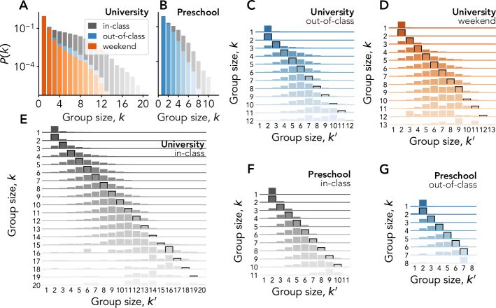
Figure 1: (A-B) Group size distributions for University (A) and Preschool (B) interactions that take place in-class, out-of-class, or during the weekend (see legend). (C-G) Node transition matrix for University (C-E) and Preschool (F-G), for interactions that take place during in-class (E,F), out-of-class (C,G), or weekend (D) time. The elements of each matrix represent the conditional probability $P(n_{i}^{t+1}=k^{\prime}|n_{i}^{t}=k)$ of finding a node $i$ in a group of size $k^{\prime}$ at time $t+1$ given that at time $t$ it belonged to a different group of size $k$. Probability values are given by the height of each element (normalized by row). Note that the scales on the y-axes–one for each matrix row–vary for visualization purposes.

Extracting groups from real-world data

We consider records from two data-collection efforts that tracked social interactions at a university and in a preschool, yielding data sets in the form of temporal networks, in which each person is represented as a node and each interaction as a temporal edge (see Materials and Methods). Time is in each case discretized by the temporal resolution of the data collection setup. At each timestamp, we define as groups the maximal cliques (largest fully connected subgraphs) and build in this way a temporal hypergraph. At each timestamp, each node can thus be either isolated or part of one or several groups (hyperedges).

University.

We use data collected by the Copenhagen Network Study (CNS) Sapiezynski et al. (2019). It is a temporally-resolved data describing the proximity events of 706 freshmen students at the Technical University of Denmark, collected using the exchange of Bluetooth signals by their smartphones. We use the publicly available data describing these proximity events during four consecutive weeks and with a temporal resolution of $5$ minutes Sapiezynski et al. (2019). We split the data into three different contexts, which might result in different interaction patterns. First, we treat all interactions taking place over the weekends as a separate set. Second, we divide interactions that happen during the workweek into in-class and out-of-class time. In this way, we do not mix the group dynamics emerging in unconstrained interactions during the free time of the lunch break and in-between classes with potentially constrained co-presence due to common attendance of classes and/or seating configurations. For this data set moreover, we perform some data pre-processing before extracting the groups in each timestamp, to filter out very weak interactions (based on the Bluetooth Received Signal Strength Indication), smoothen intermittent patterns, remove spurious connections, and perform a standard triadic closure procedure with tailored parameters Sekara et al. (2016). Additional details on the data set and the pre-processing are described in the Materials and Methods.

Preschool.

We also consider another data set, collected in a preschool as part of the DyLNet project Dai et al. (2022) to follow the social interactions of children of age $3-6$ and their teachers and assistants. The data describes proximity social interactions between $174$ children and $34$ adults in seven classes, recorded by Radio Frequency Identification (RFID) Wireless Proximity Sensors carried by each participant. Interactions were recorded with a temporal resolution of $5$ seconds, during periods of $5$ consecutive days, for $10$ consecutive months (overall $50$ days of data collection) of a single academic year in a French pre-school. For the purpose of our study we rely on a pre-processed data set shared in Dai et al. (2022) and a temporal network reconstructed from the cleaned interaction signals as explained in Dai et al. (2020), and we remove the data of interactions with and between adults, to focus on the childrens’ group dynamics.

Similarly to the university setting, we also divide the data according to the contexts that may impose different constraints on the emergence of possible group interactions. We differentiate between in-class periods, during which the social grouping of children was strongly influenced by the teachers’ instructions and scheduled activities, and out-of-class periods, when children could choose freely to interact with anyone from their own and potentially other classes. For more details on the data pre-processing, network reconstruction, and context selection, we refer to the Materials and Methods section.

The higher-order dynamics of group-changing

A first coarse summary of the complexity of group interactions is documented through the heterogeneity of groups sizes, already documented in a variety of studies Patania et al. (2017); Benson et al. (2018); Cencetti et al. (2021); Iacopini et al. (2022); Korbel et al. (2023); Mancastroppa et al. (2023). We confirm this finding in the data sets considered here in Fig. 1A,B, with distributions of instantaneous group sizes having similar shape but spanning varying ranges of values: the interactions measured in the university (panel A) feature larger group sizes than preschool ones (panel B), possibly because of the longer range of the Bluetooth signals used in the data collection infrastructure. In addition, we observe a general tendency of gathering in smaller groups in contexts where students or children are free to interact (out-of-class and weekend).

The distribution of sizes is however, by design, an aggregated observable that does not inform us about the dynamics of interactions: a given node might belong at different times to groups of very different sizes, just as a node in a temporal network might have very different numbers of neighbours or centrality values at different times Braha and Bar-Yam (2006, 2009); Pedreschi et al. (2020). We thus now investigate how individuals move across groups of various sizes. We refer here to a group change by a node in the most general sense, i.e., it does not necessarily mean that the node is actively changing from a group to another one: from the point of view of a given individual, a group change can also be due to another person joining or leaving their current group. We thus build for each context a transition matrix $T\equiv\{T_{kk^{\prime}}\}$ describing these changes as measured in the data: denoting by $n_{i}^{t}$ the size of a group to which node $i$ belongs at time $t$, each matrix element represents the conditional probability $P(n_{i}^{t+1}=k^{\prime}|n_{i}^{t}=k)$ of finding a given node $i$ in a group of size $k^{\prime}$ at time $t+1$ given that at time $t$ it belonged to a different group of size $k$ (see Materials and Methods). The results, displayed in Fig. 1C-G, show strikingly robust patterns across the different contexts, differing only in the cut-off associated with the largest group sizes observed: (i) at given group size $k$ at $t$, the most probable group size at the next time step is $k^{\prime}=k$, for small enough $k$ (except for $k=1$ in which case the next size is most often $2$); (ii) the distribution $P(n_{i}^{t+1}=k^{\prime}|n_{i}^{t}=k)$ extends to values around the diagonal $k^{\prime}=k$, with both events of individuals moving to a larger or a smaller group but in both cases large differences between $k$ and $k^{\prime}$ are rare; (iii) as $k$ increases, the distribution shifts to the left of the diagonal, i.e., it becomes increasingly probable that a change of group leads an individual to a smaller group size.

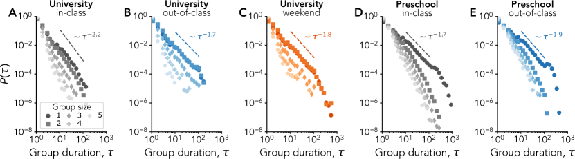
Figure 2: Distributions of group durations $\tau$ for the CNS (A-C) and the DyLNet (D-E) data sets in different contexts: in-class (A,D), out-of-class (B,E) and weekend (C). In each panel, different symbols correspond to different group sizes. The distributions for group size $1$ have been fitted using the method in Ref. Alstott et al. (2014), and can be characterized by the depicted exponent values.

Having described the evolution between groups of different sizes from an individual standpoint, we now shift the focus to a group point of view. For each group, we define its times of birth and death respectively as the first and last appearance of the same set of members in consecutive time steps. The duration of a group is then naturally given by the temporal difference $\tau$ between its time of birth and death, and we investigate in Fig. 2 how the duration statistics depend on the group size. We find that the distributions of group duration $P_{k}(\tau)$ for groups of size $k$ present broad shapes for all $k$, with comparable patterns in shape, exponent values and size dependency across the very different contexts considered. In particular, whether students interact during classes, in the other spaces of the university, or elsewhere during the weekend, the distributions of their group interactions depend on the group size in a similar way: the heavy-tail distributions are broader for smaller group sizes, with longer averages and maximum observed durations. Group interactions at preschool show a similar pattern. This extends the results described in Zhao et al. (2011) to very different contexts, showing that the strong robustness of statistical patterns of contacts goes beyond the one of pairwise interactions described in earlier works Cattuto et al. (2010); Barrat et al. (2014), and hinting at common robust mechanisms determining contact and group formation and evolution in different contexts.

To go further, we now investigate how groups change: indeed, the node transition matrices introduced above and shown in Fig. 1 give only partial information regarding the actual group dynamics. The individual point of view adopted is useful to understand how people move between group sizes, but the impact of these individual changes on the sizes of the groups needs an independent analysis. For instance, while Fig. 2 shows that larger groups tend to have shorter lives, how they break up is still to uncover. Similarly, a group might appear due to the fusion of two pre-existing groups of comparable sizes—like water droplets that merge after overlapping due to surface tension, or from a gradual process of the integration of one individual at a time. To investigate this issue, we follow the members of each group, before the group’s birth and after its break-up. Moreover, we pool together the results of groups of the same size, to check whether groups of different sizes undergo different aggregation and disaggregation dynamics. For each group size $k$, we show in Fig. 3 the heatmaps (one for each context) of the size distributions of the largest sub-set of group members observed just before the birth or just after the death of a group (see Materials and Methods). For small group sizes, both group aggregation and disaggregation tend to happen gradually from or to groups of similar sizes. This is in agreement with previous results for the formation of 3-body interactions Cencetti et al. (2021). For increasingly larger groups, the picture evolves in a slightly context-dependent way: even if no merging from (or splitting into) equally sized groups is observed, medium- and large-sized groups tend to acquire and lose members in chunks instead of one by one. This points towards a partially hierarchical dynamical mechanism according to which individuals first engage in relatively small groups that then aggregate and form bigger ones. A symmetric process takes place when large groups dismantle—first into smaller medium-sized subgroups and then loosing members one at the time.

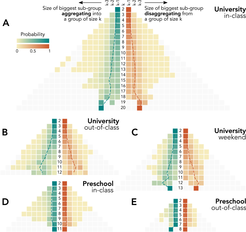
Figure 3: Group dynamics of aggregation and disaggregation for University (A-C) and Preschool (D-E) interactions that take place during in-class (A,D), out-of-class (B,E), or weekend (C) time. Each side of the pyramidal heatmaps shows the probability distribution associated to the size for the largest sub-group joining and the largest subgroup leaving a group of size $k$. The central column reports the considered group size $k$, while the probability distributions on its left-hand side and right-hand side respectively corresponds to group aggregation and disaggregation. Dashed lines refer to the distribution average.

A dynamical model for groups’ evolution

Most models describing the temporal evolution of social interactions consider network representations, i.e., are based on mechanisms describing how pairwise interactions are established and successively broken Perra et al. (2012); Starnini et al. (2013); Vestergaard et al. (2014); Karsai et al. (2014); Nadini et al. (2018); Le Bail et al. (2023). Here, we describe instead a model that explicitly integrates how individuals form groups of arbitrary sizes Stehlé et al. (2010); Zhao et al. (2011); Petri and Barrat (2018): at each time step an individual can decide to stay in their current group, leave and join a different one, or become isolated.

The model is inspired by the one put forward in Stehlé et al. (2010); Zhao et al. (2011): we consider $N$ agents $i=1,2,\dots,N$ represented as a set of vertices $\mathcal{V}$ that interact in groups over time through hyperedges. A $k$-hyperedge $\sigma\in\mathcal{K}$ is a set of $k$ vertices $\sigma=[p_{0},\dots,p_{k-1}]$ Hatcher et al. (2002) representing a group interaction of size $k$. We call $\mathcal{K}^{t}$ the set of hyperedges present at time $t$. For simplicity, we assume that each agent participates in only one hyperedge at a time. Given this rule, a useful quantity to define is $\sigma_{i}^{t}\in\mathcal{K}^{t}$, which denotes the—single—hyperedge incident on each node $i$ at time $t$, whose order $n_{i}^{t}\equiv|\sigma_{i}^{t}|$ corresponds to the size of the interaction. Under this notation, if $n_{i}^{t}=1$, node $i$ trivially forms a $1$-hyperedge with itself, which means that the agent is isolated.

The model evolves through iterations where each time step $t$ corresponds to an epoch, during which each one of the $N$ agents is selected in a random order. Whenever an agent $i\in\mathcal{V}$ is selected, currently a member of group $\sigma_{i}^{t}$, the model then evolves according to two sequential mechanisms. With the first one the agent decides to either stay in the same group, depending on the time spent there and the group size, or alternatively leave it for a different one. If the agent stays, nothing happens. If the agent instead leaves its current group, a second mechanism is triggered, corresponding to the choice of its next group: this choice is based on the acquaintances made until that time. We note that in the original model of Stehlé et al. (2010); Zhao et al. (2011), individuals leaving a group became automatically isolated, and isolated individuals could join of any size, which implies that the shape of the empirical transition matrix of Fig.1 could not be reproduced.

Let us now define these mechanisms in more details. First, we define the probability for a node $i$ to leave its own group of size $k$ at time $t$ as

$$p_{k}(\tau)=\frac{b_{k}}{\tau^{\beta}/N},$$ (1)

where $b_{k}$ is a constant that depends on the size of the current group of node $i$, $\tau$ is the time node $i$ has spent in that group (residence time), and $\beta$ is a real-valued exponent that modulates the impact of the residence time. With probability $1-p_{k}(\tau)$ the agent $i$ stays in the same group.

In case of a group change, agent $i$ leaves its current group $\sigma_{i}^{t}$ in favour of a different one $\omega\in\Omega_{t}=\{\mathcal{K}^{t}\setminus\sigma_{i}^{t}\cup\emptyset\}$. Note that, by including the empty set $\emptyset$ among the possible target groups, we account for the possibility that $i$ becomes isolated. Specifically, we include in the ensemble $\Omega_{t}$ of possible groups to join multiple copies of $\emptyset$: this multiplicity, controlled by a parameter $\epsilon$, makes it possible to tune in the model the willingness of agents to become isolated upon leaving a group. Among all possible groups $\omega\in\Omega_{t}$, $i$ selects the one to join via the second behavioural mechanism, which involves the memory of previous interactions. Namely, the probability to join $\omega$ is proportional to the fraction $\chi_{i,\omega}(t)$ of agents in $\omega$ that at time $t$ have already interacted with $i$ in the past:

$$\chi_{i,\omega}(t)=\frac{1+\Big{[}\omega\cap\bigcup\limits_{t^{\prime}=1}^{t}\sigma_{i}^{t^{\prime}}\Big{]}}{1+|\omega|}.$$ (2)

Note that node $i$ itself is included in the computation of (2) in order to have a non-zero probability for $i$ to join either an empty group or a group of previously unmet individuals. $\chi_{i,\omega}(t)$ is thus the density of agents in the group, which are known to $i$ right after joining. Altogether, the probability for an agent $i$ belonging to group $\sigma_{i}^{t}$ at time $t$ to move to group $\omega$ at time $t+1$ is given by

$$\text{Prob}(\sigma_{i}^{t+1}=\omega|\{\sigma_{i}^{t}\}_{t})=\frac{\chi_{i,\omega}(t)}{\sum_{\omega^{\prime}}\chi_{i,{\omega^{\prime}}}(t)}.$$ (3)

The inclusion of such a mechanism of social memory in the model, that translates the idea that individuals have a preference for repeating interactions with people already met, is supported by previous empirical and modelling investigations for temporal networks Karsai et al. (2014); Vestergaard et al. (2014); Le Bail et al. (2023).

Feeding the model with empirical knowledge and data

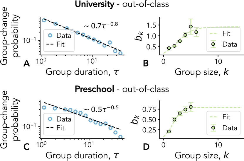
Figure 4: Fitting the empirical group-change probability for the out-of-class interactions from the CNS (A-B) and the DyLNet (C-D) data sets. (A,C) Probability for a node belonging to a group of any size to leave it for a different one after exactly $\tau$ timestamps. Points are binned empirical results, dashed lines represent a power-law fit of the form $b\tau^{\beta}$—values reported in each panel. Fitted exponents $\beta$ are then used to estimate the group-size-dependent constants $b_{k}$, as given in (1), with another power-law fit. In (B,D) the resulting values for $b_{k}$ are plotted (points) together with a logistic fit (dashed lines).

Equation (1) assumes a decreasing relationship between the probability of leaving a group of size $n$ and the time $\tau$ an agent has already spent in that group Zhao et al. (2011), i.e., a “long-gets-longer” effect. Evidence for such effect has been found empirically in pairwise interactions Vestergaard et al. (2014); Karsai et al. (2014), but the case of larger groups, and the dependency in the group size (encoded here in the set of constants $b_{k}$) have not been investigated. It is however reasonable to assume that the probability of leaving a group also depends on the size of the group itself. Indeed, size is a crucial factor that determines a group’s sociological form Simmel (1902), and its ability to sustain a single conversation —leading to the phenomenon known as schisming Egbert (1997). We thus assume, for simplicity, that $b_{k}$ increases monotonically with $k$ according to the logistic function

$$b_{k}=\frac{1}{1+e^{-\alpha(k-k_{0})}}.$$ (4)

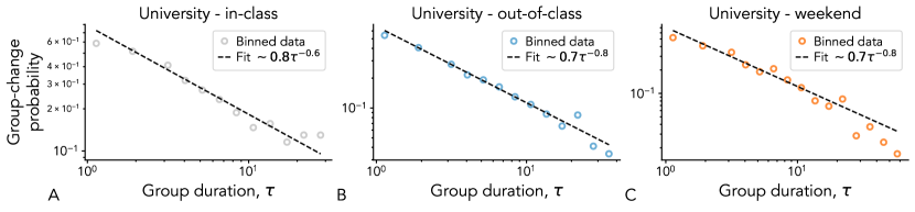
Figure S1: Fitting the group-change probability from the CNS data set by context of interaction: in-class (A), out-of-class (B), and weekend (C). We plot the probability for a node belonging to a group of any size to leave it for a different one after exactly $\tau$ timestamps. Points are binned empirical results, dashed lines represent a power-law fit of the form $b\tau^{\beta}$—values reported in each panel. Compared to Fig. S3, group sizes have been aggregated up to size $k=4$.

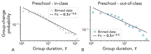
Figure S2: Fitting the group-change probability from the DyLNet data set by context of interaction: in-class (A) and out-of-class (B). We plot the probability for a node belonging to a group of any size to leave it for a different one after exactly $\tau$ timestamps. Points are binned empirical results, dashed lines represent a power-law fit of the form $b\tau^{\beta}$—values reported in each panel. Compared to Fig. S4, group sizes have been aggregated up to size $k=4$.

To validate empirically the choice of this functional form, we measure the group-change probabilities in our data, and how they depend on the group sizes. Specifically, we compute the probability $P^{\curvearrowright}(k,\tau)$ for a node belonging to a group of size $k$ to leave the group after $\tau$ timestamps (see Materials and Methods). Figure 4A,C shows the resulting probability distribution as a function of the group duration $\tau$ aggregated over all group sizes $k$ (the distributions shown in the figure correspond to interactions that take place out of class, and results for the other contexts are shown in the SI Appendix, Fig. S1 and Fig. S2). The empirical results suggest that the “old-get-older” mechanism observed in pairwise interactions remains valid for groups: the probability for an agent to change group decreases with the time they have spent in that group. In other words, the longer a group has been established, the smaller the probability that it will break apart. We fit each empirical distribution using power-law functions of the form $b\tau^{\beta}$ and report the resulting values in Fig.4A,C (dashed lines). The quality of the fit also justifies the form of (1). Similar trends can be found for the two data sets, both when aggregating over group sizes as in Fig. 4 and for the distributions $P^{\curvearrowright}(k,\tau)$ separated by group size, as shown in SI Appendix, Fig. S3 and Fig. S4 for the CNS and the DyLNet data sets, respectively.

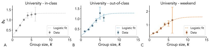
Figure S5: Estimation of the group-size-dependent constants $b_{k}$, as given in Eq. (1) of the main text, from the CNS data set by context of interaction: in-class (A), out-of-class (B), and weekend (C). For each context, the fitted exponent $\beta$ for the group-change probability reported in Fig. LABEL:fig:SI:CNS_PL_fit_group_change_by_context is used to estimate the values of $b_{k}$ for different $k$ with power-law fits. Estimated $b_{k}$ (points) are plotted together with a logistic fit (dashed lines).

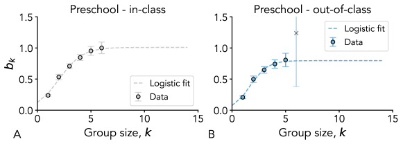
Figure S6: Estimation of the group-size-dependent constants $b_{k}$, as given in Eq. (1) of the main text, from the DyLNet data set by context of interaction: in-class (A) and out-of-class (B). For each context, the fitted exponent $\beta$ for the group-change probability reported in Fig. S2 is used to estimate the values of $b_{k}$ for different $k$ with power-law fits. Estimated $b_{k}$ (points) are plotted together with a logistic fit (dashed lines).

Using the value of $\beta$ reported in Fig. 4A,C, we finally use the fits of the empirical distributions to estimate the constants $b_{k}$ as a function of the group size for each data set and each context. We show the results in Fig.4B,D, together with the fits to a logistic form 4 (dashed lines). Similar results across the different contexts and data sets are reported in SI Appendix, Fig. S5 and Fig. S6. In all cases, the logistic fit falls within the confidence intervals of the empirical measures, justifying the choice of the logistic function assumed in the model.

The model reproduces the higher-order dynamical features

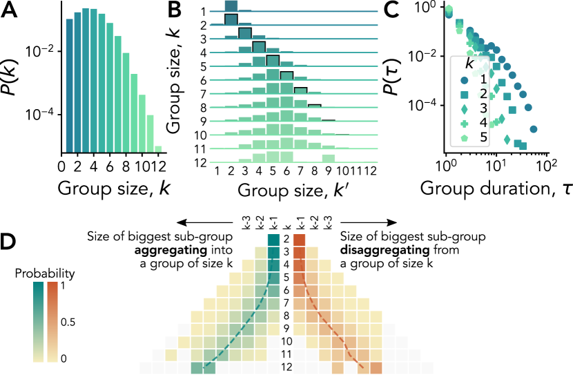
Figure 5: Simulated distribution of group size (A), node transition matrix (B), and group duration for different group sizes $k$ (C) generated by the proposed temporal hypergraph model.

We now explore the ability of the model defined above to capture the key empirical features we have uncovered in the dynamics of group interactions. As empirical results are robust across data sets and contexts, we consider as an example the University interactions taking place during out-of-class time. We thus run the model initialised with $N=700$ agents for $T=2000$ time steps, using different parameter values for $\epsilon$, $\alpha$, and $k_{0}$—while $\beta$ is set to $0.8$ as measured in Fig. 4A. Each realisation of the model generates a sequence of temporally-ordered hypergraphs that we can analyse as per the empirical data, obtaining in particular group size distributions and group size transition matrices. As described in Materials and Methods, we can thus fit the model jointly on these two observables. We show the results of the best performing model in Fig. 5. All obtained results are in line with the empirical data analysed. The group-size distribution [Fig. 5A] spans a range of values comparable with the empirical observation in Fig. 1A. The group size transition matrix for the dynamics of group changes from the node point of view, shown in Fig. 5B, has similar symmetric patterns for small sizes and a biased transition towards smaller sizes due to the cut-off effect for larger groups, as in Fig. 1C. Interestingly, other group properties, albeit not taken into account for the exploration of the model parameters, are also reproduced. Indeed, the group duration distributions (Fig. 5C) display broad tails, with a similar group size dependency as in the empirical observations of Fig. 2B. More importantly, even complex dynamical characters such as the group disaggregation and aggregation probability distributions, displayed in Figure 5D, resembles the empirical findings [Fig. 3B], showing the excellent capacity of the proposed model to account for and reproduce the complex phenomenology of the dynamics of group interactions.

Discussion

We have here analysed human interactions under the lens of group dynamics in two data sets, collected respectively among preschool children and university freshmen students. Despite the inherently different nature of their interactions due to age, contexts, and setting constraints such as class schedules, and despite the differences in data collection techniques, we have uncovered strikingly similar group dynamics both at the individual and group level. In particular, we have observed similar group size and duration distributions, and more importantly, consistent dynamical characters of individual group transitions and group formation and dissolution phenomena in the two settings and at times corresponding to different activity types. It would of course be interesting to extend these results to other contexts of human interactions, to confirm the generality of such group dynamics and patterns of group size change among humans.

Our analysis and results contribute to the obtention of a more detailed representation of social dynamics than the ones limited to pairwise interactions. We have accordingly proposed a synthetic model describing how nodes representing individuals form groups and navigate between groups of different sizes. The model includes mechanisms of short-term memory (“long gets longer”) and long-term social memory (higher probability to join a group including individuals already encountered), and is able to reproduce the non-trivial dynamics of group changes, both from a node-centric point of view and from the point of view of group formation and break-up. The model could also be extended to other forms of memory, as explored in pairwise interactions Le Bail et al. (2023).

Thanks to its realistic group dynamics, our model could be used to generate synthetic substrates for studying the impact of higher-order temporal interactions on dynamical processes. Indeed, while the impact of higher order interactions on various dynamical processes has been well assessed Iacopini et al. (2019); Battiston et al. (2021), studies on structures undergoing a realistic temporal evolution are scarce Chowdhary et al. (2021); Shang (2023). The interplay with the dynamics of groups might prove relevant for a wide variety of processes of interest in many contexts, such as the dynamics of adoption Barrat et al. (2022) and opinion formation Neuhäuser et al. (2022), but also in synchronisation Skardal and Arenas (2022); Millán et al. (2022), cooperation Traulsen and Nowak (2006) and other evolutionary dynamical processes Perc et al. (2013). Overall, our results call for the development of more modelling approaches that explicitly take both the temporal and the many-body nature of social interactions into account, both to understand the mechanisms from which the complex group dynamics emerges, and to investigate the consequences of such group gatherings in collective dynamics. Notably, such approaches should not be limited to humans, as non-human animals have also shown to be sensible to higher-order social effects Katz et al. (2011); Rosenthal et al. (2015), and, at the pairwise interaction level, complex features similar to the ones of human interactions have been observed Gelardi et al. (2020). Further studies would however be required in order to integrate behavioural response to non-pairwise interactions with additional environmental Flierl et al. (1999), cultural Conradt and Roper (2000), and ecological factors—like splitting for resource competition, or grouping as a defensive strategy against predators Wittemyer et al. (2005). Indeed, there are cases in which the drivers of animal grouping can have genetic roots Archie et al. (2006).

Another interesting research direction would be to check the robustness of the empirical results with respect to other definitions of groups or hyperedges from data obtained by measuring pairwise interactions, such as Bayesian inference approach to distinguish hyperedges from combinations of lower-order interactions Young et al. (2021), or extraction of statistically significant hyperedges Musciotto et al. (2021).

To conclude, our study contributes towards a better understanding of human behaviour in terms of the formation and disaggregation of groups, and of the navigation between social groups. We expect that the analysis presented can support researchers working at the intersection of social and behavioural sciences, while the proposed model can directly be used to inform more realistic simulations of social contagion, norm emergence, and spreading phenomena Vespignani (2012) in interacting populations.

Materials and Methods

Data Description and pre-processing

Copenhagen Network Study

We use data collected via the Copenhagen Network Study (CNS) Sapiezynski et al. (2019) that represents a temporally-resolved proximity data collected through the Bluetooth signal of cellular phones carried by 706 freshmen students at the Technical University of Denmark. The publicly available data corresponds to the data recorded during four weeks of a semester, and describes proximity of students with a temporal resolution of 5 minutes. The raw data (already pre-processed in Ref. Sapiezynski et al. (2019)) contains 5,474,289 records. Each entry contains a timestamp, the ID of one user (ego), the ID of another user (alter), and the associated Received Signal Strength Indication (RSSI) measured in dBm. The data is already processed to neglect the directionality of each interaction (which device is scanning). Empty scans (no other device found) are reported with a 0 RSSI, which corresponds to isolated nodes.

We split the data records into three main periods according to the hour of the day and the day of the week. Even though the released data Sapiezynski et al. (2019) do not contain precise information on time and date, these can be easily inferred by cross-checking activity patterns in the temporal sequences with the official timetables for Bachelor studies at DTU of Denmark (2022). The resulting contexts are:

• Workweek (in-class): Monday to Friday, 8 a.m. to 5 p.m.

• Workweek (out-of-class): Monday to Friday, 12 a.m. (midnight) to 8 a.m. and 5 p.m. to 11.59 p.m.

• Weekend: Saturday and Sunday.

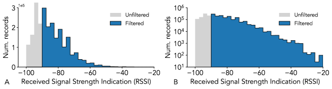
Figure S7: Filtering bluetooth signals from the CNS data set. (A) Number of recorded interactions as a function of the associated Received Signal Strength Indication (RSSI) [dBm]. The y-axis in panel (B) is in logarithmic scale. The volume of interactions retained after the filtering is displayed in blue.

We further clean the data in the following way. First, we remove external users by deleting all records in which the device of a participant scanned a device that did not take part in the experiment (resulting in 4,646,415 records). We then retain only records with an RSSI higher than -90dBm [see SI Appendix, Fig. S7]. This is slightly less restrictive than the threshold of -80dBm used in Sekara and Lehmann (2014), which was used to select interactions occurring within a radius of 2 meters (a typical distance for social interactions among close acquaintances Hall (1990)). After doing this, we have 3,824,052 records divided into 1,603,916 pairwise interactions and 2,220,136 empty scans. We treat the latter as isolated nodes.

We then perform three pre-processing steps as in Ref. Sekara et al. (2016). First, in order to smooth the pairwise interactions, we look for all the gaps composed by pairwise interactions that are present at times $t-1$ and $t+1$ but not at time $t$. We fill the resulting 163,349 gaps by using the mean RSSI of the adjacent timestamps (eventually replacing, if present, a record of an empty scan from one of the two interacting nodes).

Second, we filter out spurious interactions by removing all the 130,935 pairwise signals that are present solely at time $t$ but not at times $t-1$ and $t+1$, leaving us with 3,855,139 records. This is also in line with the procedure performed in Ref. Sekara et al. (2016), which is based on the convention developed by the Rochester Interaction Record Reis and Wheeler (1991), according to which an encounter needs to last 10 minutes or longer to be classified as meaningful.

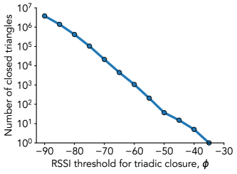
Figure S8: Pre-processing of the CNS dataset: triadic closure. Number of links added via triadic closure as a function of their approximated Received Signal Strength Indication (RSSI).

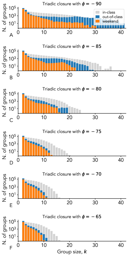
Figure S9: Pre-processing of the CNS dataset: triadic closure with threshold. Impact of thresholding the newly added link—due to the triadic closure—on the group size distributions for different contexts of interaction. Each panel shows the number of groups, divided by context [in-class (gray), out-of-class (blue), weekend (orange)], as a function of the group size $k$. Different panels (rows) correspond to different value of the threshold $\phi$ used to filter out the links added with the triadic closure. Links featuring a Received Signal Strength Indication (RSSI) [dBm] lower than $\phi$ are thus removed.

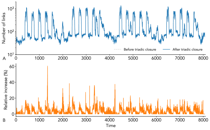
Figure S10: Preprocessing of the CNS dataset: impact of the triadic closure on the number of raw pairwise interactions in time (A), and relative change (B).

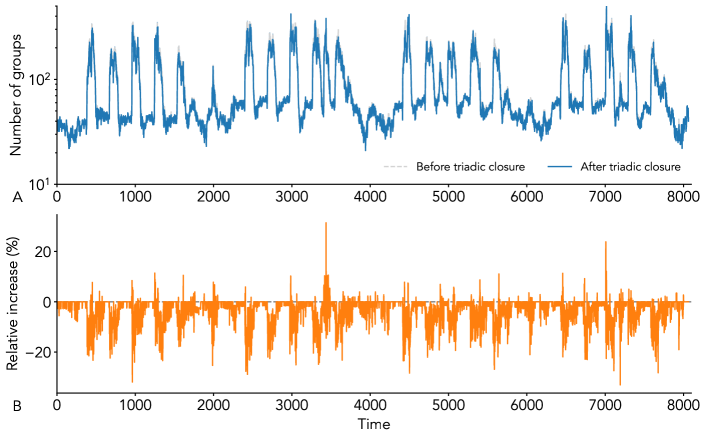
Figure S11: Preprocessing of the CNS dataset: impact of the triadic closure on the number of groups in time (A), and relative change (B).

Third, we perform triadic closure. Namely, if at time $t$ a user $i$ scans a user $j$ and user $j$ scans a user $k$, then we also add a record (if not already present) of an active scan between user $i$ and user $k$. We assign to this interaction the minimum RSSI between the other two. One of the potential pitfalls of performing triadic closure is the addition of many links to events that have already a low RSSI. In particular, if we filter the number of newly added links—due to the triadic closure—by RSSI, we notice that this number scales as a power law with the RSSI [see SI Appendix, Fig. S8]. In order to avoid closing triangles associated to “weak” events, we select an additional threshold of $-75dBm$ for the RSSI of the newly added links. This is chosen as the lowest threshold that preserves the group-size distribution across the different contexts [see SI Appendix, Fig. S9]. Figures SI Appendix, Fig. S10 and SI Appendix, Fig. S11 show the impact of the triadic closure—with the chosen threshold—on the number of links and groups in time, respectively. When observed through time, the added links by themselves do not significantly affect the number of tracked links, but help reducing the number of groups—merging together components that would be disconnected otherwise.

As a final step, we check whether the links removed during the procedure involved were the only interactions of an involved node at that particular time (also considering the triadic closure). In this case, we add back the node to the records and declare it as isolated. We finally end up with a pre-processed data set of 3,991,329 records.

DyLNet Study

The DyLNet data set was collected with the purpose of observing longitudinally the co-evolution of social network and language development of children in pre-school age. The data collection was carried out in a French preschool by recording the proxy social interactions and voice of 174 children between age 3 to 6 and their teachers and assistants. In this study we rely on data openly shared in Dai et al. (2022) and focus on the proximity social interaction data that was recorded over 9 sessions (5 morning and 4 afternoon periods— there are no classes in France on Wednesdays) per week, in 10 consecutive months during a single academic year. The data collection was carried out by using autonomous Radio Frequency Identification (RFID) Wireless Proximity Sensors (employing IEEE 802.15.4 low-rate wireless standard to communicate) installed on participants. Ground-truth data was collected in situ or via controlled experimental settings. Badges broadcasted a ‘hello’ packet with 0 dBm transmission power for 384 $\mu s$ every 5 seconds, otherwise they were in listening mode to record the badge ID and RSSI of other proxy badges if the received signal reached the minimum sensitivity value of -94 dBm. Mutually observed badges were paired to indicate proximity interactions, and were further pre-processed to finally obtain an undirected temporal network Dai et al. (2020). Interactions in this network indicate face-to-face proximity of participants within 2 meters with temporal resolution of 5 seconds.

Taking the reconstructed network Dai et al. (2022) as a starting point, we remove teachers from the data, restricting our attention to children. The data are also enriched with information. For example, the record of each pairwise interaction comes with a 5 digits label that tracks the context category of each of the two individuals at the beginning and end of the interaction. Leveraging this information, as well as the identity and class membership of each individual, as per the CNS, allows us to split interactions into two categories:

• in-class: interactions among children belonging to the same class that starts and finish during class time. Spurious interactions of children belonging to different classes during class time or interactions that start in class and end during the free time are thus removed;

• out-of-class: interactions among children of any class that start and finish during the free time. Spurious interactions that start in class and end during free time or viceversa are thus removed.

Differently from the CNS data set, no data collection was performed over the weekends. Although the resolution of the original data is 5 seconds, since there was no central unit synchronising the clocks of the badges attached to each participant (they were in-sync only once per a day), we remove interactions that last for less than 10 seconds. Finally, differently from the CNS, the DyLNet data records do not explicitly include isolated participants, i.e., a child that a given timestamp does not participate to any interaction. We thus “add back” isolated records for each child in all those timestamps in which that child does not interact with other nodes, but such that the child had at least one interaction during the same school session.

Computing node transition matrices

The node transition matrices measure the conditional probabilities of moving across groups of different sizes. Each matrix is constructed —from a node-centric point of view— by counting, for each node $i\in\mathcal{V}$, the number of observed transitions at consecutive times across two different groups of sizes $k$ and $k^{\prime}$. With the variable $n_{i}^{t}$ denoting the size of the group to which $i$ belong at time $t$, each element $T_{kk^{\prime}}$ of the matrix $T$ corresponds to the following conditional probability:

$$\begin{split}T_{kk^{\prime}}&\equiv P(n_{i}^{t+1}=k^{\prime}|n_{i}^{t}=k)\\ &=\frac{\sum_{t,i}\delta_{n_{i}^{t}k}\delta_{n_{i}^{t+1}k^{\prime}}(1-\delta_{\sigma_{i}^{t}\sigma_{i}^{t+1}})}{k^{\prime}\sum_{k^{\prime},t,i}\delta_{n_{i}^{t}k}\delta_{n_{i}^{t+1}k^{\prime}}(1-\delta_{\sigma_{i}^{t}\sigma_{i}^{t+1}})},\end{split}$$ (5)

where $\sigma_{i}^{t}$ denotes the group where node $i$ belongs at time $t$ and $\delta_{x,y}$ is the Kronecker delta function ($\delta_{x,y}=1$ if $x=y$ and zero otherwise). The normalization by the size of the target group in (5) ensures that changes to groups of different sizes are comparable. Without this, a single node leaving a group of, say, 5 nodes —assuming no further changes to the group— would result in 4 contributions (the remaining nodes) to the transitions from size 5 to size 4.

Computing group aggregation and disaggregation matrices

Studying group aggregation and disaggregation helps us to understand how groups that form/dismantle behave just before/after the event. Each group interaction $\sigma$, of size $k\equiv|\sigma|$, is associated to a time of birth $t_{\beta}$ and a time of death $t_{\delta}$ defining a temporal span $\tau=t_{\delta}-_{\beta}$ in which all the members of the group stayed continuously together. To study the aggregation and disaggregation phases, we look at how the $k$ members of $\sigma$ were respectively distributed among groups at $t_{\beta}-1$ and $t_{\delta}+1$ (if these timestamps are present within the considered context of interaction). In particular, the probability heatmaps shown in Fig. 3 are constructed, for each group size $k$, from the frequencies of the sizes of the maximal sub-groups of $\sigma$ right before its birth,

$$\max\limits_{\sigma^{\prime}\in\mathcal{K}^{t_{\beta}-1}:|\sigma^{\prime}|<|\sigma|}|\sigma\cap\sigma^{\prime}|,$$ (6)

and right after its death,

$$\max\limits_{\sigma^{\prime}\in\mathcal{K}^{t_{\delta}+1}:|\sigma^{\prime}|<|\sigma|}|\sigma\cap\sigma^{\prime}|.$$ (7)

Notice how we intentionally restrict our attention to the sub-groups of smaller sizes, thus splitting the dynamics into groups that either grow or shrink. Within this dichotomy, for example, a group of size 3 that detaches from a group of size 5 will not contribute to building the probability distribution associated to the aggregation dynamics for $k=3$, but only to the disaggregation one for $k=5$.

Computing group-change probabilities

The group-change probability for each data set and context of interaction is computed by considering for all time steps $t$ and all nodes $i$ the number of times each node, belonging to a group of size $k$, leaves the group after $\tau$ timestamps, over all the possible times. This is defined as:

$$P^{\curvearrowright}(k,\tau)=\frac{\sum\limits_{t,i}(1-\delta_{\sigma_{i}^{t+1}\sigma_{i}^{t}})\prod\limits_{\Delta=0}^{\tau+1}\delta_{\sigma_{i}^{t}\sigma_{i}^{t-\Delta}}(1-\delta_{\sigma_{i}^{t}\sigma_{i}^{t-\tau}})\delta_{n_{i}^{t}k}}{\sum\limits_{t,i}\prod\limits_{\Delta=0}^{\tau+1}\delta_{\sigma_{i}^{t}\sigma_{i}^{t-\Delta}}(1-\delta_{\sigma_{i}^{t}\sigma_{i}^{t-\tau}})\delta_{n_{i}^{t}k}}.$$ (8)

Fig. 4 shows the results aggregated over all group sizes, while the full results from (8) are given in SI Appendix, Fig. S3 and Fig. S4.

Model parametrization and fitting

The model is fitted by selecting the best-performing run among different combinations of parameters and with respect to two target observables. We perform different realisations of the model for different values of the parameters $\theta=\{\epsilon,\alpha,n_{0}\}$, while keeping constant $N=700$ (as the number of students at the university), $\beta=0.8$ (as measured, see Fig. 4), and for a number of time steps equals to $T=2000$ (notice that each time step involves the activation of every node in a random order). The optimal set of parameters $\theta^{*}$ is selected based on a joint minimisation of the Kullback–Leibler (KL) divergence $D_{\text{KL}}(\cdot||\cdot)$ with respect to the logarithm of the empirical group-size distribution $\hat{\text{P}}(k)$ and the node transition matrix $\hat{T}_{kk^{\prime}}$:

$$\begin{split}\theta^{*}=&\operatorname*{arg\,min}_{\theta}\Big{[}\mu D_{\text{KL}}\big{(}\hat{\text{P}}(k)||P(k|\theta)\big{)}\\ &+[1-\mu]D_{\text{KL}}\big{(}\hat{T}_{kk^{\prime}}||T(kk^{\prime}|\theta)\big{)}\Big{]},\end{split}$$ (9)

with $\mu=1/2$.

Data and Code Availability

The Copenhagen Network Study data are available from the original source Sapiezynski et al. (2019) at https://doi.org/10.6084/m9.figshare.7267433. The DyLNet data are available at the original source Dai et al. (2022) at https://doi.org/10.7303/syn26560886.

The code will shortly be available at https://github.com/iaciac/temporal-group-interactions . The model was coded using the XGI Python library for compleX Group Interactions Landry et al. (2023).

Acknowledgements

The authors are thankful for the insightful discussion with Sicheng Dai about the DyLNet data set. I.I. acknowledges support from the James S. McDonnell Foundation $21^{\text{st}}$ Century Science Initiative Understanding Dynamic and Multi-scale Systems - Postdoctoral Fellowship Award. A.B. and M.K. acknowledge support from the Agence Nationale de la Recherche (ANR) project DATAREDUX (ANR-19-CE46-0008). MK was supported by the CHIST-ERA project SAI: FWF I 5205-N; the SoBigData++ H2020-871042; and EMOMAP CIVICA projects.

Supplemental Material:
The temporal dynamics of group interactions in higher-order social networks

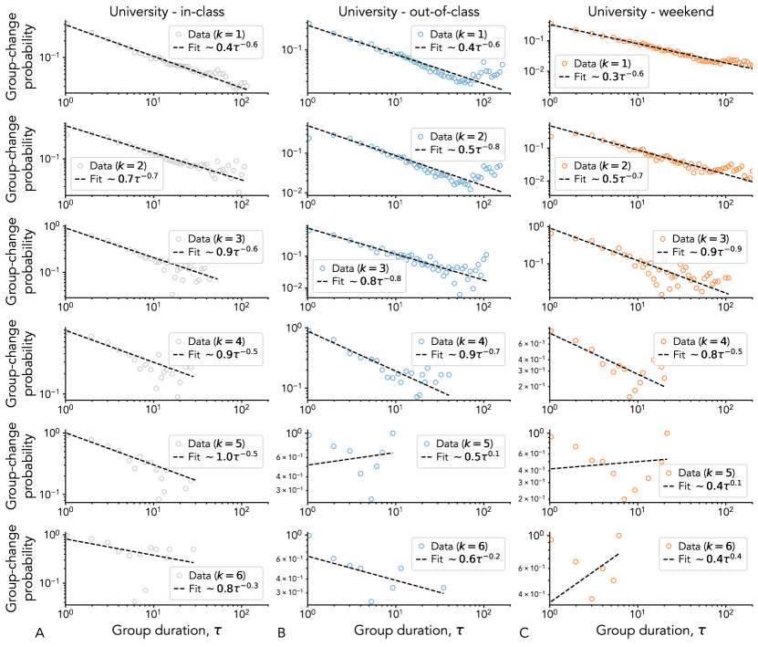
Figure S3: Fitting the group-change probability from the CNS data set by group size $k$ and by context of interaction: in-class (A), out-of-class (B), and weekend (C). Each row corresponds to a different size $k$ of the group interaction. We plot the probability for a node belonging to a group of size $k$ to leave it for a different one after exactly $\tau$ timestamps. Points are binned empirical results, dashed lines represent a power-law fit of the form $b\tau^{\beta}$—values reported in each panel.

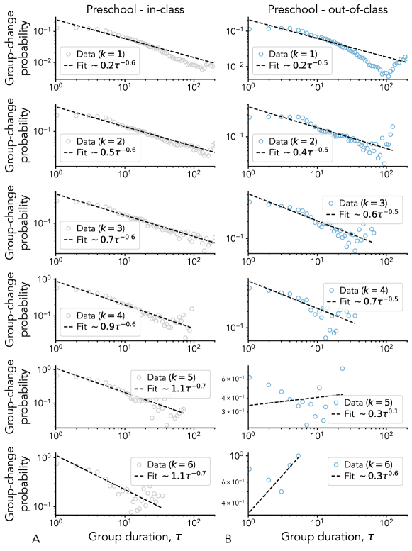
Figure S4: Fitting the group-change probability from the DyLNet data set by group size $k$ and by context of interaction: in-class (A) and out-of-class (B). Each row corresponds to a different size $k$ of the group interaction. We plot the probability for a node belonging to a group of size $k$ to leave it for a different one after exactly $\tau$ timestamps. Points are binned empirical results, dashed lines represent a power-law fit of the form $b\tau^{\beta}$—values reported in each panel.

References

- Wasserman and Faust (1994) S. Wasserman and K. Faust, Social Network Analysis: Methods and Applications, Structural Analysis in the Social Sciences (Cambridge University Press, 1994).
- Lehmann et al. (2007) Julia Lehmann, Amanda H Korstjens, and Robin IM Dunbar, “Group size, grooming and social cohesion in primates,” Anim. Behav. 74, 1617–1629 (2007).
- Dunbar (2018) Robin IM Dunbar, “The anatomy of friendship,” Trends Cogn. Sci. 22, 32–51 (2018).
- Dunbar (2020) RIM Dunbar, “Structure and function in human and primate social networks: Implications for diffusion, network stability and health,” Proc. R. Soc. A 476, 20200446 (2020).
- Albert and Barabási (2002) Réka Albert and Albert-László Barabási, “Statistical mechanics of complex networks,” Rev. Mod. Phys. 74, 47 (2002).
- Newman (2003) Mark EJ Newman, “The structure and function of complex networks,” SIAM review 45, 167–256 (2003).
- Barrat et al. (2008) A. Barrat, M. Barthélemy, and A. Vespignani, Dynamical Processes on Complex Networks (Cambridge University Press, 2008).
- Latora et al. (2017) V. Latora, V. Nicosia, and G. Russo, Complex Networks: Principles, Methods and Applications, Complex Networks: Principles, Methods and Applications (Cambridge University Press, 2017).
- Vespignani (2018) Alessandro Vespignani, “Twenty years of network science,” (2018).
- Holme and Saramäki (2012) Petter Holme and Jari Saramäki, “Temporal networks,” Phys. Rep. 519, 97–125 (2012).
- Holme (2015) Petter Holme, “Modern temporal network theory: a colloquium,” Eur. Phys. J. B 88, 1–30 (2015).
- Battiston et al. (2020) F. Battiston, G. Cencetti, I. Iacopini, V. Latora, M. Lucas, A. Patania, J.-G. Young, and G. Petri, “Networks beyond pairwise interactions: Structure and dynamics,” Phys. Rep. 874, 1–92 (2020).
- Battiston et al. (2021) F. Battiston, E. Amico, A. Barrat, G. Bianconi, G. Ferraz de Arruda, B. Franceschiello, I. Iacopini, S. Kéfi, V. Latora, Y. Moreno, M. Murray, T. Peixoto, F. Vaccarino, and G. Petri, “The physics of higher-order interactions in complex systems,” Nat. Phys. 17, 1093–1098 (2021).
- Torres et al. (2021) Leo Torres, Ann S Blevins, Danielle Bassett, and Tina Eliassi-Rad, “The why, how, and when of representations for complex systems,” SIAM Rev. 63, 435–485 (2021).
- Bianconi (2021) Ginestra Bianconi, Higher-Order Networks, Elements in Structure and Dynamics of Complex Networks (Cambridge University Press, 2021).
- Milojević (2014) Staša Milojević, “Principles of scientific research team formation and evolution,” Proc. Natl. Acad. Sci. U.S.A. 111, 3984–3989 (2014).
- Juul et al. (2022) Jonas L Juul, Austin R Benson, and Jon Kleinberg, “Hypergraph patterns and collaboration structure,” arXiv preprint arXiv:2210.02163 (2022), https://doi.org/10.48550/arXiv.2210.02163.
- Katz et al. (2011) Yael Katz, Kolbjørn Tunstrøm, Christos C Ioannou, Cristián Huepe, and Iain D Couzin, “Inferring the structure and dynamics of interactions in schooling fish,” Proc. Natl. Acad. Sci. U.S.A. 108, 18720–18725 (2011).
- McGrath (1984) J.E. McGrath, Groups: Interaction and Performance (Prentice-Hall, 1984).
- Patania et al. (2017) Alice Patania, Giovanni Petri, and Francesco Vaccarino, “The shape of collaborations,” EPJ Data Sci. 6, 1–16 (2017).
- Benson et al. (2018) Austin R Benson, Rediet Abebe, Michael T Schaub, Ali Jadbabaie, and Jon Kleinberg, “Simplicial closure and higher-order link prediction,” Proc. Natl. Acad. Sci. U.S.A. 115, E11221–E11230 (2018).
- Cencetti et al. (2021) Giulia Cencetti, Federico Battiston, Bruno Lepri, and Márton Karsai, “Temporal properties of higher-order interactions in social networks,” Sci. Rep. 11, 1–10 (2021).
- Iacopini et al. (2022) Iacopo Iacopini, Giovanni Petri, Andrea Baronchelli, and Alain Barrat, “Group interactions modulate critical mass dynamics in social convention,” Commun., Phys. 5, 1–10 (2022).
- Korbel et al. (2023) Jan Korbel, Simon D. Lindner, Tuan Minh Pham, Rudolf Hanel, and Stefan Thurner, “Homophily-based social group formation in a spin glass self-assembly framework,” Phys. Rev. Lett. 130, 057401 (2023).
- Forsyth (2018) Donelson R Forsyth, Group dynamics (Cengage Learning, 2018).
- Geard and Bullock (2010) Nicholas Geard and Seth Bullock, “Competition and the dynamics of group affiliation,” Adv. Complex Syst. 13, 501–517 (2010).
- Lotito et al. (2022) Quintino Francesco Lotito, Federico Musciotto, Alberto Montresor, and Federico Battiston, “Higher-order motif analysis in hypergraphs,” Commun. Phys. 5, 1–8 (2022).
- Mancastroppa et al. (2023) Marco Mancastroppa, Iacopo Iacopini, Giovanni Petri, and Alain Barrat, “Hyper-cores promote localization and efficient seeding in higher-order processes,” arXiv preprint arXiv:2301.04235 (2023), https://doi.org/10.48550/arXiv.2301.04235.
- Zhao et al. (2011) Kun Zhao, Juliette Stehlé, Ginestra Bianconi, and Alain Barrat, “Social network dynamics of face-to-face interactions,” Phys. Rev. E 83, 056109 (2011).
- Ceria and Wang (2023) Alberto Ceria and Huijuan Wang, “Temporal-topological properties of higher-order evolving networks,” Sci. Rep. 13 (2023), https://doi.org/10.1038/s41598-023-32253-9.
- Gallo et al. (2023) Luca Gallo, Lucas Lacasa, Vito Latora, and Federico Battiston, “Higher-order correlations reveal complex memory in temporal hypergraphs,” arXiv preprint arXiv:2303.09316 (2023), https://doi.org/10.48550/arXiv.2303.09316.
- Sekara et al. (2016) Vedran Sekara, Arkadiusz Stopczynski, and Sune Lehmann, “Fundamental structures of dynamic social networks,” Proc. Natl. Acad. Sci. U.S.A. 113, 9977–9982 (2016).
- Castellano et al. (2009) Claudio Castellano, Santo Fortunato, and Vittorio Loreto, “Statistical physics of social dynamics,” Rev. Mod. Phys. 81, 591 (2009).
- Vespignani (2012) Alessandro Vespignani, “Modelling dynamical processes in complex socio-technical systems,” Nat. Phys. 8, 32–39 (2012).
- Pastor-Satorras et al. (2015) Romualdo Pastor-Satorras, Claudio Castellano, Piet Van Mieghem, and Alessandro Vespignani, “Epidemic processes in complex networks,” Rev. Mod. Phys. 87, 925–979 (2015).
- Vestergaard et al. (2014) Christian L Vestergaard, Mathieu Génois, and Alain Barrat, “How memory generates heterogeneous dynamics in temporal networks,” Phys. Rev. E 90, 042805 (2014).
- Iacopini et al. (2019) Iacopo Iacopini, Giovanni Petri, Alain Barrat, and Vito Latora, “Simplicial models of social contagion,” Nat. Commun. 10, 2485 (2019).
- St-Onge et al. (2022) Guillaume St-Onge, Iacopo Iacopini, Vito Latora, Alain Barrat, Giovanni Petri, Antoine Allard, and Laurent Hébert-Dufresne, “Influential groups for seeding and sustaining nonlinear contagion in heterogeneous hypergraphs,” Commun. Phys. 5, 1–16 (2022).
- Papanikolaou et al. (2022) Nikos Papanikolaou, Giacomo Vaccario, Erik Hormann, Renaud Lambiotte, and Frank Schweitzer, “Consensus from group interactions: An adaptive voter model on hypergraphs,” Phys. Rev. E 105, 054307 (2022).
- Chowdhary et al. (2021) Sandeep Chowdhary, Aanjaneya Kumar, Giulia Cencetti, Iacopo Iacopini, and Federico Battiston, “Simplicial contagion in temporal higher-order networks,” J. Phys. Complexity 2, 035019 (2021).
- Sapiezynski et al. (2019) Piotr Sapiezynski, Arkadiusz Stopczynski, David Dreyer Lassen, and Sune Lehmann, “Interaction data from the copenhagen networks study,” Sci. Data 6, 1–10 (2019).
- Dai et al. (2022) Sicheng Dai, Hélène Bouchet, Márton Karsai, Jean-Pierre Chevrot, Eric Fleury, and Aurélie Nardy, “Longitudinal data collection to follow social network and language development dynamics at preschool,” Sci. Data 9, 1–17 (2022).
- Dai et al. (2020) Sicheng Dai, Hélène Bouchet, Aurélie Nardy, Eric Fleury, Jean-Pierre Chevrot, and Márton Karsai, “Temporal social network reconstruction using wireless proximity sensors: model selection and consequences,” EPJ Data Sci. 9, 19 (2020).
- Alstott et al. (2014) Jeff Alstott, Ed Bullmore, and Dietmar Plenz, “powerlaw: a python package for analysis of heavy-tailed distributions,” PLoS One 9, e85777 (2014).
- Braha and Bar-Yam (2006) Dan Braha and Yaneer Bar-Yam, “From centrality to temporary fame: Dynamic centrality in complex networks,” Complexity 12, 59–63 (2006).
- Braha and Bar-Yam (2009) Dan Braha and Yaneer Bar-Yam, “Time-dependent complex networks: Dynamic centrality, dynamic motifs, and cycles of social interactions,” in Adaptive networks: Theory, models and applications (Springer, 2009) pp. 39–50.
- Pedreschi et al. (2020) Nicola Pedreschi, Christophe Bernard, Wesley Clawson, Pascale Quilichini, Alain Barrat, and Demian Battaglia, “Dynamic core-periphery structure of information sharing networks in entorhinal cortex and hippocampus,” Netw. Neurosci. 4, 946–975 (2020).
- Cattuto et al. (2010) Ciro Cattuto, Wouter Van den Broeck, Alain Barrat, Vittoria Colizza, Jean-François Pinton, and Alessandro Vespignani, “Dynamics of person-to-person interactions from distributed rfid sensor networks,” PLoS One 5, e11596 (2010).
- Barrat et al. (2014) Alain Barrat, Ciro Cattuto, Alberto Eugenio Tozzi, Philippe Vanhems, and Nicolas Voirin, “Measuring contact patterns with wearable sensors: methods, data characteristics and applications to data-driven simulations of infectious diseases,” Clin. Microbiol. Infect. 20, 10–16 (2014).
- Perra et al. (2012) Nicola Perra, Bruno Gonçalves, Romualdo Pastor-Satorras, and Alessandro Vespignani, “Activity driven modeling of time varying networks,” Sci. Rep. 2, 1–7 (2012).
- Starnini et al. (2013) Michele Starnini, Andrea Baronchelli, and Romualdo Pastor-Satorras, “Modeling human dynamics of face-to-face interaction networks,” Phys. Rev. Lett. 110, 168701 (2013).
- Karsai et al. (2014) Márton Karsai, Nicola Perra, and Alessandro Vespignani, “Time varying networks and the weakness of strong ties,” Sci. Rep. 4, 1–7 (2014).
- Nadini et al. (2018) Matthieu Nadini, Kaiyuan Sun, Enrico Ubaldi, Michele Starnini, Alessandro Rizzo, and Nicola Perra, “Epidemic spreading in modular time-varying networks,” Sci. Rep. 8, 1–11 (2018).
- Le Bail et al. (2023) Didier Le Bail, Mathieu Génois, and Alain Barrat, “Modeling framework unifying contact and social networks,” Phys. Rev. E 107, 024301 (2023).
- Stehlé et al. (2010) Juliette Stehlé, Alain Barrat, and Ginestra Bianconi, “Dynamical and bursty interactions in social networks,” Phys. Rev. E 81, 035101 (2010).
- Petri and Barrat (2018) Giovanni Petri and Alain Barrat, “Simplicial activity driven model,” Phys. Rev. Lett. 121, 228301 (2018).
- Hatcher et al. (2002) A. Hatcher, Cambridge University Press, and Cornell University. Department of Mathematics, Algebraic Topology, Algebraic Topology (Cambridge University Press, 2002).
- Simmel (1902) Georg Simmel, “The number of members as determining the sociological form of the group,” Am. J. Sociol. 8, 1–46 (1902).
- Egbert (1997) Maria M Egbert, “Schisming: The collaborative transformation from a single conversation to multiple conversations,” Res. Lang. Soc. 30, 1–51 (1997).
- Note (1) Note that similar group duration distributions were actually already found in a different context Zhao et al. (2011).
- Shang (2023) Yilun Shang, “Non-linear consensus dynamics on temporal hypergraphs with random noisy higher-order interactions,” J. Complex Netw. 11, cnad009 (2023).
- Barrat et al. (2022) Alain Barrat, Guilherme Ferraz de Arruda, Iacopo Iacopini, and Yamir Moreno, “Social contagion on higher-order structures,” in Higher-Order Systems (Springer, 2022) pp. 329–346.
- Neuhäuser et al. (2022) Leonie Neuhäuser, Renaud Lambiotte, and Michael T Schaub, “Consensus dynamics and opinion formation on hypergraphs,” in Higher-Order Systems (Springer, 2022) pp. 347–376.
- Skardal and Arenas (2022) Per Sebastian Skardal and Alex Arenas, “Explosive synchronization and multistability in large systems of kuramoto oscillators with higher-order interactions,” in Higher-Order Systems (Springer, 2022) pp. 217–232.
- Millán et al. (2022) Ana Paula Millán, Juan G Restrepo, Joaquín J Torres, and Ginestra Bianconi, “Geometry, topology and simplicial synchronization,” in Higher-Order Systems (Springer, 2022) pp. 269–299.
- Traulsen and Nowak (2006) Arne Traulsen and Martin A. Nowak, “Evolution of cooperation by multilevel selection,” Proc. Natl. Acad. Sci. U.S.A. 103, 10952–10955 (2006), https://www.pnas.org/doi/pdf/10.1073/pnas.0602530103 .
- Perc et al. (2013) Matjaž Perc, Jesús Gómez-Gardenes, Attila Szolnoki, Luis M Floría, and Yamir Moreno, “Evolutionary dynamics of group interactions on structured populations: a review,” J. R. Soc. Interface 10, 20120997 (2013).
- Rosenthal et al. (2015) Sara Brin Rosenthal, Colin R Twomey, Andrew T Hartnett, Hai Shan Wu, and Iain D Couzin, “Revealing the hidden networks of interaction in mobile animal groups allows prediction of complex behavioral contagion,” Proc. Natl. Acad. Sci. U.S.A. 112, 4690–4695 (2015).
- Gelardi et al. (2020) Valeria Gelardi, Jeanne Godard, D. Paleressompoulle, N. Claidière, and A. Barrat, “Measuring social networks in primates: wearable sensors versus direct observations,” Proc. R. Soc A 476, 20190737 (2020).
- Flierl et al. (1999) G Flierl, D Grünbaum, S Levin, and D Olson, “From individuals to aggregations: the interplay between behavior and physics,” J. Theor. Biol. 196, 397–454 (1999).
- Conradt and Roper (2000) Larissa Conradt and Timothy J Roper, “Activity synchrony and social cohesion: a fission-fusion model,” Proc. Royal Soc. B 267, 2213–2218 (2000).
- Wittemyer et al. (2005) George Wittemyer, Iain Douglas-Hamilton, and Wayne Marcus Getz, “The socioecology of elephants: analysis of the processes creating multitiered social structures,” Anim. Behav. 69, 1357–1371 (2005).
- Archie et al. (2006) Elizabeth A Archie, Cynthia J Moss, and Susan C Alberts, “The ties that bind: genetic relatedness predicts the fission and fusion of social groups in wild african elephants,” Proc. Royal Soc. B 273, 513–522 (2006).
- Young et al. (2021) Jean-Gabriel Young, Giovanni Petri, and Tiago P Peixoto, “Hypergraph reconstruction from network data,” Commun. Phys. 4, 135 (2021).
- Musciotto et al. (2021) Federico Musciotto, Federico Battiston, and Rosario N Mantegna, “Detecting informative higher-order interactions in statistically validated hypergraphs,” Commun. Phys. 4, 218 (2021).
- of Denmark (2022) Technical University of Denmark, “Course base,” https://www.dtu.dk/english/education/course-base (2022).
- Sekara and Lehmann (2014) Vedran Sekara and Sune Lehmann, “The strength of friendship ties in proximity sensor data,” PLoS One 9, e100915 (2014).
- Hall (1990) E.T. Hall, The Hidden Dimension (Anchor Books, 1990).
- Reis and Wheeler (1991) Harry T. Reis and Ladd Wheeler, “Studying social interaction with the rochester interaction record,” Adv. Exp. Soc. Psychol. 24, 269–318 (1991).
- Landry et al. (2023) Nicholas W. Landry, Maxime Lucas, Iacopo Iacopini, Giovanni Petri, Alice Schwarze, Alice Patania, and Leo Torres, “Xgi: A python package for higher-order interaction networks,” J. Open Source Softw. 8, 5162 (2023).