Neural Volumetric Reconstruction for Coherent Synthetic Aperture Sonar

Abstract.

Synthetic aperture sonar (SAS) measures a scene from multiple views in order to increase the resolution of reconstructed imagery. Image reconstruction methods for SAS coherently combine measurements to focus acoustic energy onto the scene. However, image formation is typically under-constrained due to a limited number of measurements and bandlimited hardware, which limits the capabilities of existing reconstruction methods. To help meet these challenges, we design an analysis-by-synthesis optimization that leverages recent advances in neural rendering to perform coherent SAS imaging. Our optimization enables us to incorporate physics-based constraints and scene priors into the image formation process. We validate our method on simulation and experimental results captured in both air and water. We demonstrate both quantitatively and qualitatively that our method typically produces superior reconstructions than existing approaches. We share code and data for reproducibility.

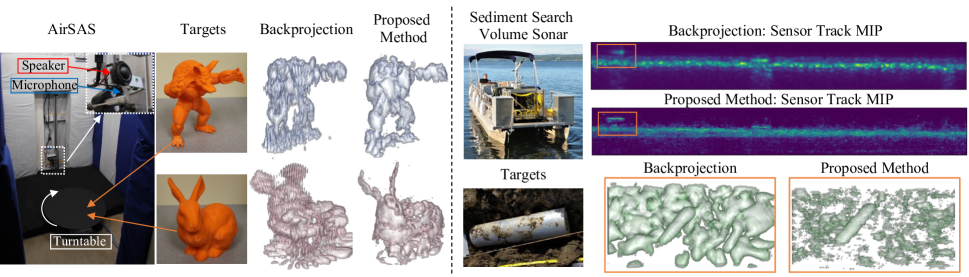
Figure 1. We propose an analysis-by-synthesis optimization that leverages techniques from neural rendering to optimize coherent reconstructions of SAS volumetric scenes. We demonstrate our approach on an in-lab circular SAS in air (AirSAS) and in-water bistatic SAS, the sediment volume search sonar (SVSS). On the left side of the figure, we show the AirSAS, 3D printed targets, and reconstructions obtained using backprojection and our proposed method. On the right side, we show 2D maximum intensity projections (MIPs) of the SVSS track and 3D reconstructions of targets highlighted in orange. In many cases, our method produces better reconstructions than traditional SAS reconstruction algorithms, such as backprojection. SVSS hardware photos courtesy of (Brown et al., 2021).

This is a teaser figure

1. Introduction

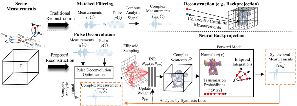
Figure 2. Block diagram of our method. Given measurements obtained from $n$ sensor positions, the top row shows the traditional reconstruction pipeline and the bottom row shows our proposed reconstruction pipeline. Traditional reconstruction uses matched filtering to compress the measurements in time, and then coherently combines measurements using backprojection (or a functionally equivalent algorithm implemented in the Fourier domain). Our method roughly parallels these steps. Instead of matched filtering, we apply pulse deconvolution, which is an optimization that deconvolves the transmitted pulse from measurements. We then propose neural backprojection, which uses a neural network to estimate the scene and synthesizes measurements using our differentiable forward model. The network is trained by minimizing a loss between synthesized and pulse deconvolved measurements.

Synthetic aperture sonar (SAS) is an active acoustic imaging technique that coherently combines data from a moving array to form high-resolution imagery, especially of underwater environments (Bellettini and Pinto, 2008; Hayes and Gough, 2009). The moving array in SAS collects both magnitude and phase information which allows coherent integration methods to achieve resolution parallel to the sensor path that is independent of range (Callow, 2003). These high resolution SAS reconstructions are important for applications in target localization (Williams, 2016), monitoring man-made (Nadimi et al., 2021) and biological structures (Sture et al., 2018).

However, reconstructing SAS imagery from measurements is an under-constrained problem (Callow, 2003). First, SAS scenes are often undersampled due to the slow propagation of sound relative to the traveling velocity of the sensor platform (Callow, 2003; Putney and Anderson, 2005). Second, SAS transducers (transmitter and receiver) are bandlimited, limiting the ability to reconstruct arbitrarily fine spatial frequencies in imagery (de Heering et al., 1994; Reed et al., 2022; Pailhas et al., 2017).

In related fields, under-constrained imaging problems are typically addressed by optimizing an objective function that incorporates scene or physics-based priors into the reconstruction (Bouman, 2022). In particular, a common strategy is analysis-by-synthesis, where a forward model synthesizes measurements from an estimated scene, and the scene is optimized by minimizing the loss between synthesized and given measurements (Bertero et al., 2021; Lucas et al., 2018). This framework can flexibly incorporate losses corresponding to sensor noise models and custom scene priors (Kaipio and Somersalo, 2004). State-of-the-art analysis-by-synthesis typically uses a neural network coupled with a differentiable forward map (Xie et al., 2022). Notably, neural radiance fields (NeRF) use a neural network and differentiable volume rendering to synthesize novel views of 3D scenes from 2D images (Mildenhall et al., 2021).

Despite the success of these methods, existing SAS reconstruction algorithms do not use analysis-by-synthesis optimization for reconstruction. Instead, SAS reconstruction coherently combines measurements (in either the time or frequency domain) to focus acoustic energy into the scene. While post-processing optimizations are used (e.g. image-space deconvolution (Reed et al., 2022; de Heering et al., 1994; Pailhas et al., 2017), autofocus (Marston et al., 2014; Mansour et al., 2018; Fienup, 2000; Gerg and Monga, 2020)), these methods seek to improve already reconstructed SAS images, rather than incorporate the physics and priors into the image formation.

The challenge for analysis-by-synthesis reconstructions for SAS is the lack of differentiable forward models that are computationally efficient. Acoustic rendering by solving wave equations is physically-realistic but computationally expensive. While geometric acoustic renderers exist for simulating SAS measurements (Gul et al., 2017; Woods, 2020), they are not typically differentiable. Further, since SAS measurements can be collected on arbitrary paths (Callow, 2003; Hayes and Gough, 2009) (although they typically align with circular or linear scans in practice), it is difficult to precompute a simple forward model. Moreover, SAS arrays transmit spherically propagating sources and measure time series of the received sound pressure. This requires more burdensome sampling than in the optical domain, where cameras measure the intensity of a light ray that travels in a straight line, typically without phase information. These challenges must be taken into account when designing a forward model for analysis-by-synthesis optimization.

Inspired by recent neural rendering techniques, we design an analysis-by-synthesis method for coherent SAS reconstruction. We leverage implicit neural representations (pioneered by NeRF (Mildenhall et al., 2021)) to estimate acoustic scatterers in a 3D volume. Specifically, we formulate a differentiable forward map of a point-based sonar scattering model, and design an ellipsoidal sampling technique to importance sample propagating acoustic pressure waves and then synthesize measurements. Our analysis-by-synthesis optimization allows us to incorporate the physics of the measurement formation, various noise models, and scene priors into the reconstruction. We demonstrate that our technique is not restricted to any particular spatial sampling pattern.

Our proposed method consists of two primary steps. First, we leverage iterative pulse deconvolution to perform pulse compression which increases the bandwidth of the emitters and sensors computationally. Second, we propose an analysis-by-synthesis reconstruction algorithm, which we term neural backprojection. Our method is inspired by traditional NeRF techniques but varies significantly in terms of sampling (ellipsoidal vs. line sampling) and output (intensity vs. time series). We perform multiple experiments on simulated and hardware-measured data to show both quantitatively and qualitatively that our design outperforms traditional techniques. Using ablation studies, we validate our design and contextualize the performance of our method against existing approaches. Our specific contributions are as follows:
(1) An analysis-by-synthesis framework for incorporating the physics of acoustic signal formation, scene priors, and noise models for coherent volumetric SAS reconstructions. 
(2) Design of a differentiable acoustic forward model that assumes ideal pulse deconvolution to sample along constant time-of-flight ellipsoids.
(3) Evaluation of our proposed method on simulated and real hardware measurements from an in-air circular SAS and in-water measurements from a field survey of a lakebed using a bistatic SAS.
(4) Code and datasets, shared as supplementary material and on the website, for reproducibility.

Organization:

The rest of the paper is organized as follows. Section 2 provides background on SAS and existing reconstruction methods. Section 3 introduces our forward model and provides background on how it is traditionally inverted. Section 4 gives a summary of our proposed approach, which involves pulse deconvolution (Section 5) and neural backprojection (Section 6). Section 7 discusses our datasets and code implementation. Section 8 validates our method by comparing it to existing reconstruction methods and through extensive ablations on hardware measured and simulated data. Section 9 discusses the main findings, impact, and limitations of our work, along with potential future directions.

2. Related Work

2.1. Synthetic Aperture Sonar (SAS)

Many sensing modalities leverage a combination of spatially distributed measurements to enhance performance. In particular, array or aperture processing use either a spatial array of sensors (i.e. real aperture) or a virtual array from moving sensors (i.e. synthetic aperture) to reconstruct a spatial map of the scene. Synthetic aperture imaging has been used for sonar and radar (Gough and Hawkins, 1997b), ultrasound (Jensen et al., 2006) and optical light fields (Levoy and Hanrahan, 1996). Synthetic aperture imaging techniques parallel many of those in tomographic imaging which leverage penetrating waves to image the target scene (Ferguson and Wyber, 2009).

In this paper, we focus on synthetic aperture sonar (SAS) which is a leading technology for underwater imaging and visualization (Hayes and Gough, 2009). Acoustical waves are used to insonify the scene, and the time-of-flight of the acoustic signal is used to help determine the location of target objects and scatterers in the scene. Exploiting the full resolution of synthetic aperture systems requires coherent integration of measurements — combination considering measurement magnitude and phase (Hawkins, 1996). In particular, coherent integration yields an along-track (along the sensor path) resolution independent of range and wavelength (Hawkins, 1996).

SAS systems typically transmit pulse compressable waveforms, waveforms with large average power but with good range resolution (Eaves and Reedy, 2012; Harrison, 2019). Common examples include swept frequency waveforms, which apply a linear or non-linear change in waveform frequency over time (Harrison, 2019). These waveforms are pulse compressed at the receiver by correlating measurements with the transmitted waveform (i.e., pulse). This processing is commonly referred to throughout communications and remote sensing communities as matched filtering (or replica-correlation). Waveform design is an active areas of research for creating optimal compressed waveforms — there is a tradeoff between range resolution and hardware limitations affecting bandwidth (Callow, 2003).

2.2. SAS Reconstruction

Many algorithms exist for reconstructing imagery from SAS measurements. Perhaps the most intuitive algorithm is time-domain backprojection (also called delay-and-sum or time-domain correlation) which backprojects received measurements to image voxels using their time-of-flight measurements. The advantage of this method is that it works for arbitrary scanning geometries, however, traditionally it has been considered slow to compute (Hayes and Gough, 2009; Soumekh, 1999). Wavenumber domain algorithms such as range-Doppler and $\omega-k$ migration are significantly faster but require assuming a far-field geometry and an interpolation step to snap measurements onto a Fourier grid (Eaves and Reedy, 2012; Hayes and Gough, 2009). For circular scanning geometries (CSAS), specialized reconstruction algorithms (Plotnick et al., 2014; Marston et al., 2011, 2014) exploit symmetry and connections to computed tomography (Ferguson and Wyber, 2005) for high-resolution visualization. Even further specialized SAS techniques leverage interferometry (Hansen et al., 2003; Griffiths et al., 1997) for advanced seafloor mapping. In this paper, we use time-domain backprojection as our baseline SAS reconstruction approach. While this method is considered slow conventionally, modern computing capabilities with GPUs have alleviated this bottleneck (Gerg et al., 2020). Backprojection is applicable to nearly arbitrary measurement patterns, in contrast with Fourier-based methods which make a collocated transmit/receive assumption and require interpolation to a Fourier grid. Additionally, backprojection and Fourier methods typically produce equivalent imagery for data that meets the requirements necessary of the Fourier-based algorithms (Bamler, 1992).

Many methods exist for further improving the visual quality of reconstructed imagery. Notably, many methods estimate the platform track and motion to correct imaging errors (Cook, 2007; Brown et al., 2019a; Yu et al., 2006; Cook and Brown, 2008; Fienup, 2000; Callow, 2003; Fortune et al., 2001),deconvolution (Putney and Anderson, 2005; de Heering et al., 1994), autofocus (Marston et al., 2014; Gerg and Monga, 2021), and accounting for environment noise (Chaillan et al., 2007; Callow, 2003; Hayes and Gough, 1992; Piper et al., 2002). These methods are complementary to our reconstruction approach, and could be investigated further in conjunction with our pipeline.

2.3. Acoustic Rendering

Modeling acoustic information in an environment has largely fallen into two broad categories: geometric acoustics and wave-based simulation. Geometric acoustic methods, also known as ray tracing, are based upon a small wavelength approximation to the wave equation (Savioja and Svensson, 2015; Liu and Manocha, 2020). The analog of Kajiya’s rendering equation for room acoustics has been proposed with acoustic bidirectional reflectance distributions (Siltanen et al., 2007). Further, bidirectional path tracing has been introduced to handle occlusion in complex environments (Cao et al., 2016). However, diffraction can cause changes in sound propogation, particularly near edges where sound paths bend. To account for this, researchers have proposed techniques to add these higher-order diffraction effects to path tracing and radiosity simulations (Schissler et al., 2014).

In contrast, solving the wave equation directly encapsulates all these diffraction effects, but is computationally expensive (Hamilton et al., 2017). To alleviate processing times, precomputation has been used extensively (Raghuvanshi et al., 2010; Raghuvanshi and Snyder, 2014) with these systems. In addition, acoustic textures have been introduced to enable fast computation of wave effects for ambient sound and extended sources (Zhang et al., 2018b, 2019). Further, anisotropic effects for complex directional sources can be rendered efficiently (Chaitanya et al., 2020). In addition to acoustically modeling large environments, there has been a large body of work modeling the vibration modes of complex objects (Wang et al., 2018). This includes elastic rods (Schweickart et al., 2017), fire (Chadwick and James, 2011), fractures (Zheng and James, 2010), thin shells (Chadwick et al., 2009).

For SAS in particular, there have been several acoustic rendering models proposed in the literature. The Personal Computer Shallow Water Acoustic Tool-set (PC-SWAT) is a common underwater simulation environment that leverages finite element modeling (Sammelmann, 2001) as well as extensions to ray-based geometric acoustics (Woods, 2020). HoloOcean is a more general underwater robotics simulator that enables simulation of acoustics (Potokar et al., 2022). BELLHOP is a popular acoustic ray tracing model for long range propagation modeling (Gul et al., 2017). In this work, we leverage the Point-based Sonar Scattering Model (PoSSM), a single bounce acoustic scattering model (Brown et al., 2017; Brown, 2017; Johnson and Brown, 2018), to design our forward model for our neural backprojection method.

2.4. Transient and Non-Line-of-Sight Imaging

Many works use optical transient imaging for measuring scenes in depth by leveraging continuous wave time-of-flight devices (Heide et al., 2013; Kadambi et al., 2016, 2013) or impulse-based time-of-flight single photon avalanche diode (SPADs) (O’Toole et al., 2017; Callenberg et al., 2021). In particular, transient imaging is useful for non-line-of-sight (NLOS) reconstruction (Velten et al., 2012; Arellano et al., 2017; Lindell et al., 2019b; Ahn et al., 2019; Liu et al., 2019; Pediredla et al., 2019). Analysis-by-synthesis optimization has been effective for NLOS problems including differentiable transient rendering (Iseringhausen and Hullin, 2020; Yi et al., 2021; Plack et al., 2023; Wu et al., 2021) and even utilized for conventional cameras (Chandran and Jayasuriya, 2019; Chen et al., 2019). While there are interesting connections between transient/NLOS imaging and SAS, more research is needed to connect these domains. Lindell et al. used acoustic time-of-flight to perform NLOS reconstruction (Lindell et al., 2019a), but do not consider SAS processing. SAS imaging presents new technical challenges for transient imaging including non-linear measurement trajectories and bi-static transducer arrays, coherent processing, and acoustic-specific effects.

2.5. Neural Fields

Recently, there has been large interest in representing scenes or physical quantities using the optimized weights of neural networks (Xie et al., 2022). These networks, termed implicit neural representations (INR), or more broadly as neural rendering or neural fields, exploded in popularity following NeRF, which used them for learning 3D volumes from 2D images (Mildenhall et al., 2021). These networks use a positional encoding to overcome spectral bias (Cao et al., 2019).

INRs have been used in a huge number of inverse problems across imaging and scientific applications (Xie et al., 2022). In particular, INRs have been recently applied to tomographic imaging methods which has similarities to synthetic aperture processing (Sun et al., 2022; Zang et al., 2021; Rückert et al., 2022; Reed et al., 2021b). Of particular interest to our work is neural rendering for time-of-flight (ToF) cameras. Time-of-Flight Radiance Fields couples a ToF camera with an optical camera to create depth reconstructions (Attal et al., 2021). While this work does consider the phase of the ToF measurements, their method does not feature coherent integration of phase values as we do in synthetic aperture processing. Further, they consider ToF cameras where each pixel corresponds to samples along a ray. In contrast, measurements from a SAS array correspond to samples along propagating spherical wavefronts. Shen et al. propose leveraging neural fields for NLOS imaging (Shen et al., 2021). In contrast, we leverage neural fields coupled with differentiable acoustic forward model for SAS imaging.

Several works consider apply neural fields for sonar and SAS image reconstruction. Reed et al. leverage neural fields to perform 2D CSAS deconvolution (Reed et al., 2021a, 2022). Their method post-processes (deblurs) reconstructed 2D scenes for circular SAS measurement geometries (Reed et al., 2022). On the other hand, our proposed approach focuses on reconstruction for 3D SAS. Recently, a method using an INR for forward-looking sonar was developed (Qadri et al., 2023). Forward-looking sonar stitches images together from individual slices, and does not typically utilize coherent integration. Our method differs from this method as we account for the effects of the transmit waveform and consider the coherent integration of multiple views, which is fundamental to synthetic aperture processing.

3. Background: Forward Model and Time-Domain Backprojection

Table 1. Definition of operators and variables used throughout the paper.

Operators	Definition
$\widehat{x}$	Complex-valued analytic signal of $x$.
—x—	Magnitude of $x$. If $x=a+jb$ then $|x|=\sqrt{a^{2}+b^{2}}$.
$\angle x$	Angle of $x$. If $x=a+jb$ then $\angle x=\tan^{-1}{b/a}$.
——x——	2-norm of vector $\mathbf{x}$.
$\mathcal{H}(x)$	Hilbert transform of $x$.
$\mathcal{R}(x)$	Real part of $x$.
$\mathcal{I}(x)$	Imaginary part of $x$.
Variables
$p(t)$	Transmitted pulse.
$s_{n}(t)$	Raw measurements of sensor $n$.
$s_{{\text{MF}}}(t)$	Match-filtered measurements.
$s_{\text{PD}}(t)$	Given Pulse deconvolved measurements .
$\mathbf{s^{\prime}}_{\text{PD}}(t)$	Synthesized pulse deconvolved measurements.
$N_{\text{PD}}$	Pulse deconvolution network.
$N_{\text{BP}}$	Neural backprojection network.
$\Delta f$	Transmit pulse bandwidth.
$f_{\text{start}}$	Transmit pulse start frequency.
$f_{\text{stop}}$	Transmit pulse stop frequency.
$f_{c}$	Transmit pulse center frequency, $(f_{\text{start}}+f_{\text{stop}})/2$.
$\mathcal{X}$	The set of all scene points.
$\mathbf{E}_{r_{i}}$	The set of points $x$ on the ellipsoid surface at range $r_{i}$.
$b_{T}(\mathbf{x})$	Transmitter directivity function at point $\mathbf{x}.$
$b_{R}(\mathbf{x})$	Receiver directivity function at point $\mathbf{x}.$
$a(r_{i})$	Length of ellipsoid $x$ semi-axis defined at range $r_{i}$.
$b(r_{i})$	Length of ellipsoid $y$ semi-axis defined at range $r_{i}$.
$c(r_{i})$	Length of ellipsoid $z$ semi-axis defined at range $r_{i}$.
$\mathbf{o}_{T}$	Transmitter origin.
$\mathbf{x}_{T}$	Transmission ray.
$\mathbf{o}_{R}$	Receiver origin.
$\mathbf{x}_{R}$	Receive ray.
$\mathbf{d}_{T}$	Transmit ray direction (unit vector).
$T(\mathbf{o}_{T},\mathbf{x})$	Transmission probability from a transmitter origin to a point $\mathbf{x}$.
$T(\mathbf{o}_{R},\mathbf{x})$	Transmission probability from a receiver origin to a point $\mathbf{x}$.
$r_{i}$	Distance $i$ from transmit and receiver origin.
$l_{i}$	Depth $i$ along ray.
$\widehat{\sigma^{\prime}}$	Estimated complex scattering function.
$\sigma$	Ground truth scattering function.

We first introduce the forward measurement model that we use later to design our analysis-by-synthesis optimization. This model is inspired by a point-based sonar scattering model (Brown, 2017; Brown et al., 2017). Point scattering models assume high-frequency propagation (i.e., geometric acoustics), but offer computational tractability and differentiability that is friendly for neural rendering techniques.

We now formulate our imaging model mathematically (we refer the reader to Table 1 for reference to the notation used throughout the text). Let $\mathbf{x}\in\mathbb{R}^{3}$ describe a 3D coordinate in a scene, $\sigma(\mathbf{x})\in\mathbb{R}$ the amplitude of the acoustic scatterer at $\mathbf{x}$, $p(t)$ is the transmitted pulse, and $\mathcal{X}$ the set of all coordinates in the volume of interest. We also define $b_{T}(\mathbf{x})$ and $b_{R}(\mathbf{x})$ to be the transmitter and receiver directivity functions respectively. We define $T(\mathbf{o}_{T},\mathbf{x})$ and $T(\mathbf{o}_{R},\mathbf{x})$ as the transmission probabilities between a scene point and the transmitter and receiver origins, respectively, where $T(\cdot)$ is a function that computes the transmission probability between two points and enables our model to account for occlusion.

Let $R_{T}=||\mathbf{o}_{T}-\mathbf{x}||$ and $R_{R}=||\mathbf{o}_{R}-\mathbf{x}||$ be the distances between the scene point and sensor transmit and receive origins, respectively. Then, the receiver records real-valued measurements similar to Brown et al. (Brown et al., 2017):

(1) $$\mathbf{s}(t)=\int\displaylimits_{\mathcal{X}}\frac{b_{T}(\mathbf{x})b_{R}(\mathbf{x})T(\mathbf{o}_{T},\mathbf{x})T(\mathbf{o}_{R},\mathbf{x})}{2\pi R_{T}R_{R}}L(\sigma(\mathbf{x}))p\left(t-\frac{R_{t}+R_{R}}{c}\right)\mathrm{d}\mathbf{x},$$

where $L(\cdot)$ is a Lambertian acoustic scattering model computed using the normal vector at a point $\mathbf{n}(\mathbf{x})$. Contrary to acoustic radiance (Siltanen et al., 2007), this equation models acoustic pressure which has a $1/\text{distance}$ falloff due to spherical propagation (Pierce, 1981). Additionally, note that the sensor measurement $s(t)=s(\mathbf{o}_{T},\mathbf{o}_{R},t)$ is actually a function of the transmit and receive origins as well. Throughout the text, we will sometimes index measurements as $\mathbf{s}_{n}(t)$, but typically omit $n$ for brevity.

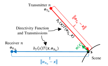
Figure 3. Forward model geometry. A transmitter pings the scene with the transmit waveform. The propagation of the waveform to a scene point $\mathbf{x}$ is weighted by the directivity function and transmission probability. The scene point reflects acoustic energy back towards the receiver that is weighted by a Lambertian scattering term, the return transmission probability, and the receiver directivity.

3.1. Conventional SAS Reconstruction with Time-domain Backprojection

We now briefly discuss the traditional processing pipeline for SAS measurements, where received measurements are compressed in range and the coherent integration of measurements forms an image.

Match-filtering and Pulse Compression.

The first processing step for the received signal is to perform matched filtering by cross-correlating with the transmitted pulse:

(2) $$\mathbf{s}_{\text{MF}}(t)=\mathbf{s}(t)\ast_{t}p^{*}(-t).$$

Note that we have written the cross-correlation as a convolution in time $\ast_{t}$ with the time-reversed conjugate signal $p^{*}(-t)$ which is typically done in sonar/radar processing literature. Match-filtering is a robust method for deconvolving the transmission waveform from measurements (Soumekh, 1999) and is the optimal linear filter for detecting a signal in white noise (Smith, 1997).

For a simple rectangular transmitted pulse $p(t)=A,-\tau/2\leq t\leq\tau/2$ and zero elsewhere, it is easy to show that $S_{MF}(t)$ is a triangle function and the energy of the signal is $A^{2}\tau$. Since the transmitter is operating at peak amplitude (in this example), the duration of the signal $\tau$ yields higher energy, and thus higher signal-to-noise ratio (SNR). However, increasing $\tau$ comes at the expense of poor range-resolution, given by the equation (Eaves and Reedy, 2012; Harrison, 2019):

(3) $$\Delta r=\frac{c}{2B},$$

where $c$ is the pulse propagation speed, and the bandwidth $B=1/\tau$ in this case.

To decouple the relationship between range resolution and energy of the signal, sonars transmit a frequency-modulated pulse (Harrison, 2019). In particular, the linear frequency modulated (LFM) pulse is a common choice:

(4) $$p(t)=w(t)\cos\left(2\pi\frac{\Delta f}{2\tau}t^{2}+2\pi f_{\text{start}}t\right),$$

where the bandwidth in Hz is given by $\Delta f$ = $|f_{\text{start}}-f_{\text{stop}}|$, $\tau$ is the pulse duration in seconds, and $w(t)$ is a windowing function to attenuate side-lobes in the ambiguity function. The range-resolution of a pulse-compressed waveform computed using Eq. (3) is $\Delta r=\frac{c}{2\Delta f}$.

Coherent Backprojection.

Synthetic aperture imaging reconstructs images with range-independent along-track resolution through coherent integration of measurements (Callow, 2003). As the transmitted waveform is typically modulated by a carrier frequency, it is desirable to coherently integrate the envelope of received measurements. The signal envelope can be estimated with range binning (Hayes and Gough, 2009), but the analytical form of the envelope is obtained with the Hilbert transform (Bracewell, 1986). In particular, the Hilbert transform can be used to obtain the analytic signal (also called the pre-envelope):

(5) $$\widehat{\mathbf{s}_{\text{MF}}}=\mathbf{s}_{\text{MF}}+j\mathcal{H}(\mathbf{s}_{\text{MF}})$$

where $j=\sqrt{-1}$ and $\mathcal{H}$ is the Hilbert transform operator.

Given these (now) complex measurements, SAS image formation uses the sensor and scene geometry to coherently integrate measurements that are projected onto the scene using their time-of-flights,

(6) $$I_{\text{BP}}(\mathbf{x})=\sum_{n}\widehat{\mathbf{s}_{\text{MF}_{n}}}\left(t-\frac{R_{T}+R_{R}}{c}\right).$$

Later, we show that this equation effectively integrates energy along ellipsoids defined by the transmit and receive locations and time-of-flights. We remind the reader that the values $R_{T},R_{R}$ are defined in terms of $\mathbf{x}$ and the transmit and receive positions of the transducers, and thus are not constant for differing $n$ and $\mathbf{x}$. Eq. (6) is the coherent integration of measurements and results in a complex image. The final estimate of the acoustic scattering coefficient $\sigma(\mathbf{x})$ is obtained by taking the image magnitude $|I_{\text{BP}}(\mathbf{x})|$ (Hawkins, 1996).

4. Overview of Proposed Method

Our proposed reconstruction method (shown in Fig. 2) consists of two main steps that roughly parallel the matched filtering and coherent backprojection described in the previous section. First, we propose deconvolving given waveforms via an iterative deconvolution optimization rather than performing matched filtering. While matched filtering can be optimized through waveform design to realize a better ambiguity function in cross-correlation (i.e. better range compression), these techniques require a priori knowledge and do not work across a variety of sonar environments. In contrast, we present an adaptable approach to waveform compression where performance can be tuned via sparsity and smoothness priors, which we label pulse deconvolution in Section 5.

Our second step is an analysis-by-synthesis reconstruction using an implicit neural representation (similar to NeRF in traditional view synthesis (Mildenhall et al., 2021)). We use a network to predict complex-valued scatterers, and use a differentiable forward model to synthesize complex sensor measurements in time. Traditional NeRF scene sampling methods are not directly applicable to our problem since we require sampling the scene points with constant time-of-flight, which correspond to ellipsoids with the transmitter and receiver as foci (Pediredla et al., 2019). Thus, we project rays from the transducer and sample rays at the intersection of ellipsoidal surfaces corresponding to measurement time bins and develop importance sampling methods to determine transmission probabilities for these rays and ellipsoidal surfaces. Finally, we explain how we implement our physics-based priors, such as a Lambertian scattering assumption, and regularization to our analysis-by-synthesis optimization.

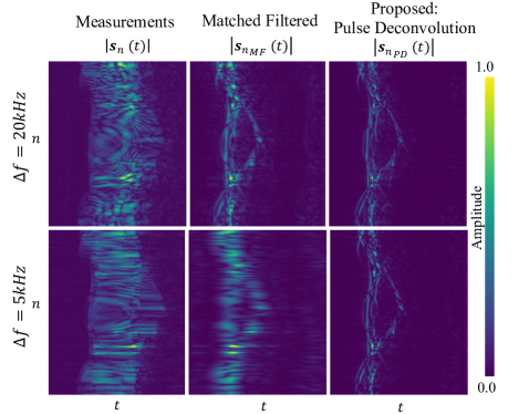
Figure 4. Comparing matched filtering performance with pulse deconvolution. We show the magnitude (i.e., signal envelope) of AirSAS measurements of a 3D-printed Stanford bunny measured with an LFM ($f_{c}=20$ kHz) at bandwidths $\Delta f=20$ kHz (top row) and $\Delta f=5$ kHz (bottom row). Matched filtering’s ability to compress measurements degrades at the lower $5$ kHz bandwidth. Our pulse deconvolution method yields better compression at both bandwidths.

5. Pulse Deconvolution

We now present our method for deconvolving the transmit waveform from SAS measurements. We refer to the deconvolved measurements as $\mathbf{s}_{\text{PD}}(t)$. We propose optimizing a network, labeled the pulse deconvolution network $N_{pd}$ as,

(7) $$\begin{split}\mathcal{L}_{PD}=||N_{PD}(t;\theta_{\text{PD}})\ast p^{*}(-t)-\mathbf{s}(t)||_{2}\\ +\lambda_{1_{\text{PD}}}\mathcal{L}_{\text{Sparse}}^{\text{PD}}+\lambda_{2_{\text{PD}}}\mathcal{L}_{\text{TV Phase}}^{\text{PD}},\end{split}$$

where $\theta_{\text{PD}}$ are the trainable weights of the network. The sparsity and phase smoothing operators are defined as,

(8) $$\mathcal{L}_{\text{Sparse}}^{\text{PD}}=\sum_{t}||N_{PD}(t;\theta_{\text{PD}})||_{1}$$

(9) $$\mathcal{L}_{\text{PD, TV Phase}}^{\text{PD}}=\sum_{t}||\nabla\angle N_{PD}(t;\theta_{\text{PD}})||_{1},$$

where $\angle\cdot$ denotes the angle of a complex value and where regularizors are weighted by scalar hyperparameters $\lambda_{1_{\text{PD}}}$ and $\lambda_{2_{\text{PD}}}$. We find that sparsity regularization is particularly important for recovering accurate deconvolutions. The total-variation (TV) phase prior encourages the solution to have a smoothly varying phase, which we find helps attenuate noise in the deconvolved waveforms. We minimize the total pulse deconvolution loss $\mathcal{L}_{PD}$ with respect to the network weights $\theta_{\text{PD}}$ using PyTorch’s ADAM (Kingma and Ba, 2014) optimizer.

We implement the network using an implicit neural representation (INR), where input coordinates are transformed with a hash-encoding (Müller et al., 2022) to help the network overcome spectral bias. Our implementation trains an INR per batch of sensor measurements. In particular, we add an additional input to the network, $n$ (omitted from Eq (9)), that denotes a sensor index and allows a single network to deconvolve a batch of sensor measurements. At inference, we form the pulse deconvolved signal $\mathbf{s}_{\text{PD}}(t)=N_{PD}(t;\theta_{\text{PD}})$ using the network and then calculate the analytic signal $\widehat{\mathbf{s}_{\text{PD}}}$ to be used for coherent neural backprojection described in Section 6.

Fig. 4 compares the pulse compression performance of match-filtering and our deconvolution method on AirSAS (Section 7.2) data. The figure shows $n=360$ bunny measurements recorded using an LFM with center frequency $f_{c}=20$ kHz at bandwidths $\Delta f=20$ kHz and $\Delta f=$ 5 kHz. In agreement with Eq. (3), match-filtering compresses measurements more at $\Delta f=20$ kHz than at $\Delta f=5$ kHz. Our proposed deconvolution method compresses the measurements more than match-filtering and with remarkably similar performance at both bandwidths.

In addition to our proposed deconvolution method, we experiment with deconvolving the waveforms in a single step using simple Wiener deconvolution, but observe notably inferior performance compared to the network. We also tried optimizing Eq. (7) without a neural network (i.e., by updating the values at each time bins directly via gradient descent) and actually observed competitive deconvolution performance. However, we find that the network seems to output marginally smoother deconvolved waveforms. Given this observation, and the fact that the INR had a nearly equivalent latency, we use a network in Eq. (7) to obtain $\mathbf{s}_{\text{PD}}(t)$ for all experiments.

6. Neural Backprojection

Our first choice for synthesizing measurements is to use the point-based scattering model of Eq. (1). However, coherent backprojection methods integrate the envelope of the signal from Eq. (1), and thus we perform our analysis-by-synthesis optimization by computing a loss between synthesized measurements and given analytic (i.e. complex) signal measurements from the data. To synthesize the analytic measurements, we derive an approximation to the analytic forward model (see the supplemental material for the full derivation):

(10) $$\widehat{\mathbf{s^{\prime}}_{\text{PD}}}\left(t=\frac{R_{T}+R_{R}}{c}\right)\approx\int_{\mathbf{E}_{r}}b_{T}(\mathbf{x})b_{R}(\mathbf{x})T(\mathbf{o}_{T},\mathbf{x})T(\mathbf{x},\mathbf{o}_{R})L({\widehat{\sigma^{\prime}}}(\mathbf{x}))\mathrm{d}\mathbf{x},$$

where $\widehat{\mathbf{s^{\prime}}_{\text{PD}}}$ are synthesized (i.e. rendered) complex-valued pulse deconvolved measurements. This equation synthesizes measurements using the transmitter and receiver directivity functions $b_{T}(\mathbf{x})$ and $b_{R}(\mathbf{x})$, the transmission probabilities to and from each point $T(\mathbf{o}_{T},\mathbf{x})$ and $T(\mathbf{x},\mathbf{o}_{R})$, and a Lambertian scattering function $L(\cdot)$ applied to complex-valued scene scatterers ${\widehat{\sigma^{\prime}}}$.

A key property of Eq. (10) is that ${\widehat{\sigma^{\prime}}}$ now defines complex-valued scatterers, which is consistent with how conventional backprojection algorithms recover a complex SAS image corresponding to the complex envelope of the matched filtered signals (Bracewell, 1986; Hayes and Gough, 1992). It also accounts for any non-idealities in the pulse deconvolution which can introduce complex magnitude and phase into the equation. Thus in Eq. (10), we are synthesizing complex-valued estimates of given deconvolved measurements such that $\mathcal{R}(\widehat{\mathbf{s^{\prime}}_{\text{PD}}})(t)\approx\mathbf{s}_{\text{PD}}(t)$. This enables us to coherently integrate scatterers and recover our estimate of the scatterers $\sigma(x)$ from Eq. (1) by computing the magnitude $|{\widehat{\sigma^{\prime}}}(\mathbf{x})|\approx\sigma(\mathbf{x})$.

In Eq. 10, the measured amplitude at a particular time is given by integrating complex-valued scatterers along a 3D ellipsoid surface $\mathbf{E}_{r}$. Assuming no multipath, the ellipsoid is defined by a constant time-of-flight from the transmitter and receiver origins (and whose sampling we detail further in Section 6.1). The ellipsoid approximation assumes that pulse deconvolution works well, and we show in our experimental results that not performing pulse deconvolution results in worse reconstructions. Finally, we note that we assume $b_{R}(\mathbf{x})$ = 1 for all $\mathcal{X}$, which is reasonable since receivers typically have relatively large beamwidths to suppress aliasing (Gough and Hawkins, 1997a), and omit the term $\frac{1}{2\pi R_{T}R_{R}}$ in the equation as this is commonly done in time-domain beamformers in actual implementation (Hayes and Gough, 1992).

We estimate the complex scattering function ${\widehat{\sigma^{\prime}}}$ using a neural network, entitled the back-projection network $N_{\text{BP}}$, that is parameterized with weights $\theta_{\text{BP}}$. Specifically, the network defines the complex scatterer at each location,

(11) $${\widehat{\sigma^{\prime}}}(\mathbf{x})=N_{\text{BP}}(\mathbf{x};\theta_{\text{BP}}).$$

Thus the analysis-by-synthesis optimization loss can be written as

(12) $$\mathcal{L}_{BP}=\left|\left|\widehat{\mathbf{s^{\prime}}_{\text{PD}}}-\widehat{\mathbf{s}_{\text{PD}}}\right|\right|_{2},$$

where we minimize the loss between complex-valued synthesized and given pulse deconvolved measurements with respect to the network weights $\theta_{\text{BP}}$ using PyTorch’s ADAM (Kingma and Ba, 2014) optimizer.

In the next subsections, we describe how we importance sample the scene via ellipsoids of constant time-of-flight (Section 6.1), estimate the transmission probabilities for the transmit and return rays and compute surface normals (Section 6.2), and compute the above loss with regularization terms (Section 6.3).

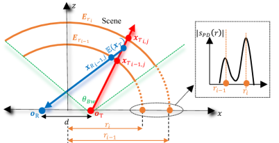
Figure 5. 2D diagram ($xz$ slice) of our sampling scheme. A transmission ray (red) is projected within the transmitter beamwidth (green) and sampled at the intersection of the ellipsoids (orange) defined by range samples (shown in the dotted black box). The return ray (blue) is computed from the expected depth of the transmit ray back to the receiver.

6.1. Ellipsoidal Sampling

As shown in Fig. 5, a set of points for a constant time-of-flight $t=\frac{R_{t}+R_{R}}{c}$ define an ellipsoid whose foci are the transmitter and the receiver positions, and with semi-major axis length $r=c\cdot t/2$, where $c$ is the sound speed. The ellipsoid can be written as:

(13) $$\frac{x^{2}}{a(r)^{2}}+\frac{y^{2}}{b(r)^{2}}+\frac{z^{2}}{c(r)^{2}}-1=0,$$

where transmit $\mathbf{o}_{T}$ and receive $\mathbf{o}_{R}$ elements are separated by distance $d$. The ellipsoid semi-axes lengths are,

(14) $$a(r)=r,b(r)=\sqrt{(r)^{2}-(d/2)^{2}},c(r)=b(r).$$

Thus, our problem reduces to sampling the intersection of transmitted and received rays with these ellipsoids. We begin by sampling a bundle of rays originating from the transmitter and within its beamwidth $\theta_{\text{bw}}$. Fig. 5 illustrates a transmitted ray in red with direction $\mathbf{d}_{{T}_{j}}$ and defined as

(15) $$\mathbf{x}_{T_{ij}}=\mathbf{o}_{T}+l_{i}\mathbf{d}_{{T}_{j}}$$

where $l_{i}$ are depth samples along the ray. We sample this ray at its intersection with ellipsoids defined by desired range of samples. Note that we index ray samples by the ray direction $j$ and the depth sample $i$.

In contrast to conventional NeRF methods that use a coarse network for depth importance sampling, we can use the time series measurements. In particular, we sample time $t_{i}$ with probability $Pr(t=t_{i})=\frac{|\widehat{\mathbf{s}_{\text{PD}}}(t_{i})|}{\sum_{i}\left|\widehat{\mathbf{s}_{\text{PD}}}(t_{i})\right|}$.

This concept is illustrated in Fig. 5. In the upper left of the figure, we show a deconvolved waveform that is sampled at two-time bins (converted to range using $r_{i}=c\cdot t_{i}/2$). These sampled ranges define ellipsoids drawn in the orange curves. We find the depth $l_{i}$ that a ray intersects the ellipsoid by substituting the ray into the ellipsoid equation. Substitution yields a quadratic equation with a positive root,

(16) $$l_{i}=-b_{0}+\frac{\sqrt{b_{0}^{2}-4a_{0}c_{0}}}{2a_{0}}$$

where

(17) $$a_{0}=\frac{[d_{T}]_{x}^{2}}{a(r_{i})^{2}}+\frac{[d_{T}]_{y}^{2}}{b(r_{i})^{2}}+\frac{[d_{T}]_{z}^{2}}{c(r_{i})^{2}}$$

(18) $$b_{0}=\frac{2[x_{T}]_{x}[d_{T}]_{x}}{a(r_{i})^{2}}+\frac{2[x_{T}]_{y}[d_{T}]_{y}}{b(r_{i})^{2}}+\frac{2[x_{T}]_{z}[d_{T}]_{z}}{c(r_{i})^{2}}$$

(19) $$c_{0}=\frac{[x_{T}]_{x}^{2}}{a(r_{i})^{2}}+\frac{[x_{T}]_{y}^{2}}{b(r_{i})^{2}}+\frac{[x_{T}]_{y}^{2}}{c(r_{i})^{2}}-1,$$

and the notation $[d_{T}]_{x}$ refers to the $x$ component of the vector $\mathbf{d}_{T}$. The positive root of the quadratic corresponds to the valid intersection, while the negative root is the intersection on the other side of the ellipsoid.

While not shown in the figure, we also implement a simple direction-based priority sampling. Specifically, we sample a set of sparse rays spanning uniform directions within the transmitter beamwidth. We integrate along each ray and use the resulting magnitude to weight the likelihood of dense sampling in nearby directions.

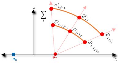
Figure 6. 2D diagram ($xz$ slice) of our scheme for integrating ellipsoid surfaces to synthesize measurements. Eq. (10) weights scene scatterers by their respective transmission and Lambertian terms and integrates them along the surface of ellipsoids.

6.2. Transmission and Normal Calculations

We handle occlusion by computing transmission probabilities between the transmitter/receiver and scene points. Our computed transmission probability is similar to NeRF’s (Mildenhall et al., 2021), although we use it to weight complex-valued scatter coefficients rather than scene density.

As shown in Fig. 6, the network $N_{\text{BP}}$ predicts complex-valued scatterers $({\widehat{\sigma^{\prime}}}_{ij})$ at the sampled ray-ellipsoid intersections. The transmission probability between the transmitter and scene point is computed using the cumulative product in depth (Mildenhall et al., 2021)

(20) $$T(\mathbf{o}_{T},\mathbf{x}_{T_{i}})=\prod_{k<i}\exp{\left(-|{\widehat{\sigma^{\prime}}}_{k}|\cdot|l_{k+1}-l_{k}|\cdot\zeta\right)},$$

where $k$ indexes depth, and we omit the direction index $j$ since Eq. (20) is computed for all rays. We use the scalar $\zeta$ to scale the transmission falloff rate — we find it useful to increase $\zeta$ for sparser pulse deconvolved waveforms (corresponding to sparser scenes). Note that we use the scatterer magnitude to compute the transmission probability since each term in the cumulative product should be non-negative.

Computing a return ray from each sampled transmission point approximately squares the number of required scene samples. Thus, we compute a return ray only from the expected depth of the transmission ray (Zhang et al., 2021). The return ray is illustrated in blue in Fig. 5. We compute the expected ray sample in-depth as,

(21) $$\mathbb{E}(\mathbf{x}_{T})=\sum_{i}\mathbf{x}_{T_{i}}\frac{|{\widehat{\sigma^{\prime}}}(\mathbf{x}_{i})T(\mathbf{o}_{T},\mathbf{x}_{T_{i}})|}{\sum_{i}|{\widehat{\sigma^{\prime}}}(\mathbf{x}_{i})T(\mathbf{o}_{T},\mathbf{x}_{T_{i}})|}.$$

and define the return ray as

(22) $$\mathbf{x}_{R_{ij}}=\mathbb{E}(\mathbf{x}_{T_{i}})+l_{i}\mathbf{d}_{R_{j}},$$

where $\mathbf{d}_{R_{j}}$ = $\frac{\mathbf{o}_{R}-\mathbb{E}(\mathbf{x}_{T_{j}})}{||\mathbf{o}_{R}-\mathbb{E}(\mathbf{x}_{T_{j}})||}$ and the depths $l_{i}$ are sampled at the ellipsoid intersections found using the negative root of Eq. (16). Since the expected depth is typically less than the max depth (see Fig. 5), we simply set return ray samples with depths greater than the expected sample (i.e. when $l<0$) to 0 so that they are ignored by downstream calculations. We compute a transmission probability for the return ray using a cumulative product in depth (Eq. 20). The return ray is used only to compute the transmission probability — its sampled points are not part of the ellipsoid surface integrations of Eq. (10). Note that for simulated and real AirSAS experiments, the transmitter and receiver are collocated so we omit calculating the transmittance of the returning ray.

We compute surface normals using a method from Poole et al. (Poole et al., 2022),

(23) $$\mathbf{n}(\mathbf{x})=\frac{\nabla\mathbf{x}|{\widehat{\sigma^{\prime}}}|}{\left|\left|\nabla\mathbf{x}|{\widehat{\sigma^{\prime}}}|\right|\right|},$$

noting that we use the magnitude of the scatterers for normal computation. Scatterers are weighted with a Lambertian scattering model model (Lambert, 1760; Ramamoorthi and Hanrahan, 2001)

(24) $$L({\widehat{\sigma^{\prime}}})={\widehat{\sigma^{\prime}}}\cdot\max\left(0,\mathbf{n}(\mathbf{x})\cdot\frac{\mathbf{x}-\mathbf{o}_{T}}{\left|\left|\mathbf{x}-\mathbf{o}_{T}\right|\right|}\right).$$

We show in our experiments that the Lambertian scattering model is important for reconstructing accurate object surfaces.

6.3. Loss and Regularization

Fig. 6 illustrates integrating sampled ellipsoid surfaces after weighting scene scatterers with transmission and Lambertian terms. As expressed in Eq. (10), these operations synthesize a complex-valued waveform. We compute a loss between the synthesized waveform and the analytic version of the pulse deconvolved waveforms,

(27) $$\begin{gathered}\mathcal{L}_{BP}=\left|\left|\widehat{\mathbf{s^{\prime}}_{\text{PD}}}-\widehat{\mathbf{s}_{\text{PD}}}\right|\right|_{2}+\\ \lambda_{1_{\text{BP}}}\mathcal{L}_{\text{Sparse}}^{\text{BP}}+\lambda_{2_{\text{BP}}}\mathcal{L}_{\text{TV}_{\text{Space}}}^{\text{BP}}+\lambda_{3_{\text{BP}}}\mathcal{L}_{\text{TV}_{\text{Phase}}}^{\text{BP}}\end{gathered}$$

where $\lambda_{1_{\text{BP}}}$, $\lambda_{2_{\text{BP}}}$, and $\lambda_{3_{\text{BP}}}$ are scalar weights for commonly used sparsity and total variation priors defined as,

(28) $$\mathcal{L}_{\text{Sparse}}^{\text{BP}}=\sum_{n}\left|\left||{\widehat{\sigma^{\prime}}}|\right|\right|_{1}$$

(29) $$\mathcal{L}_{\text{TV}_{\text{Space}}}^{\text{BP}}=\sum_{n}||\nabla_{d_{\text{reg}}}{\widehat{\sigma^{\prime}}}||_{1},$$

(30) $$\mathcal{L}_{\text{TV}_{\text{Phase}}}^{\text{BP}}=\sum_{n}||\nabla_{d_{\text{reg}}}\angle{\widehat{\sigma^{\prime}}}||_{1}.$$

The total loss is minimized with respect to the network weights. The total variation losses are performed on the complex scene scatterers and their phase — the $\nabla_{d_{\text{reg}}}$ is computed using the distance hyperparameter $d_{\text{reg}}$ that determines the distance between the compared samples. Regularization terms are computed using all ray samples. We find that these priors benefit some reconstructions while harming others and should be tuned depending on the scene and measurement noise. For example, in the supplemental material we show that these priors are particularly useful when reconstructing from limited measurements. We highlight that the ability to add and tune priors is an advantage of our method over backprojection, which does not have the ability to incorporate priors (Ahn et al., 2019).

Eq. (27) should be minimized over the given $n$ sensor measurements. In practice, we use gradient accumulation to average the gradients over a fixed number of sensors before performing a backpropagation update to the weights. We find that this stabilizes the optimization while avoiding the memory overhead of batching multiple sensors. In all experiments, we accumulate gradients over $5$ sensors.

Finally, we note that the loss function as shown in Eq. (27) can be considered coherent since it computes the loss between the complex estimated and target deconvolved measurements. In the supplemental material, we show that incoherent reconstruction yields inferior results, validating our design choice of having the network predict complex-valued scatterers and performing the loss between complex-valued measurements.

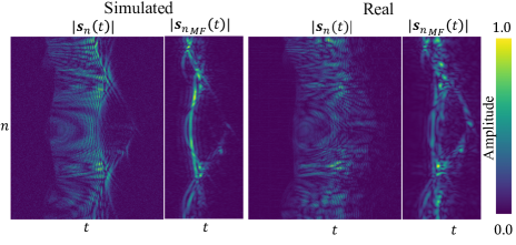
Figure 7. Comparing simulated measurements and real measurements of the bunny measured using an LFM pulse ($f_{c}=20$ kHz and $\Delta f=20$ kHz). Our simulated measurements are qualitatively similar to real measurements.

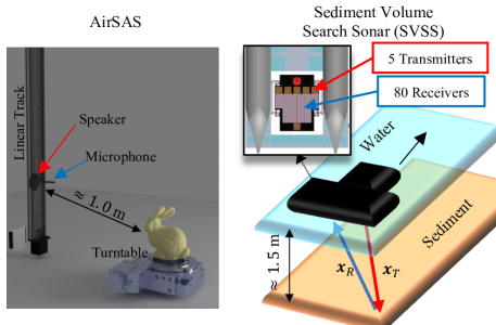
Figure 8. Measurement geometry for the AirSAS (left) and SVSS (right). AirSAS collects circular SAS measurements inside an anechoic chamber using a speaker and microphone pointed at a turntable. The speaker and microphone are mounted on a vertical linear track $1$ meter from the turntable. Objects on the turntable fit within 0.2 cubic meters. SVSS is mounted on a pontoon boat that travels in a linear fashion and is used to image underwater targets. The SVSS array is approximately $1.5$ meters above the lakebed and reconstructs scenes with dimension approximatley $1$ meter across (perpendicular to platform path) and between $1-10$ meters long (parallel to platform path).

7. Simulator and Hardware Implementation

In this section, we discuss the implementation of a simulator and hardware for collecting SAS measurements. We refer the reader to open-source code and data.

7.1. SAS Simulator using Optical Time-of-Flight Renderer

We simulate SAS measurements by leveraging an implementation of an optical time-of-flight (ToF) renderer based on Kim et al. (Kim and Kim, 2021). This renderer was chosen in part due to its CUDA implementation that uses asynchronous operations to efficiently accumulate per-ray radiances by their travel time. While this simulator does not capture acoustic effects (including diffraction), it does enable efficient prototyping and we note that optical renderers have been leveraged for SAS simulation in the literature (Reed et al., 2019).

Specifically, we configure the simulator to emulate an in-air, circular SAS setup called AirSAS (Blanford et al., 2019). AirSAS consists of a speaker and microphone directed at a circular turntable that holds a target. We simulate the speaker (transmitter) as a point light source and the microphone (receiver) with an irradiance meter to measure reflected rays. We configure the renderer to measure the ToF transients from each sensor location. We convolve these transients with our transmitted pulse to obtain simulated SAS measurements. We provide plots of rendered transient signals in the supplemental document.

We use simulated measurements for several experiments to quantitatively evaluate the effect of bandwidth, noise, and object shape. In Fig. 7, we show a side-by-side comparison of a subset of simulated and measured waveforms from the bunny. While our simulator ignores non-linear wave effects like sound diffraction and environmental effects like changing sound speed, we observe that the simulated measurements are similar to AirSAS measurements.

7.2. AirSAS

AirSAS is an in-air, circular SAS contained within an anechoic chamber (Blanford et al., 2019). AirSAS being an in-air system enables experimental control that is impossible or challenging to achieve in water. Importantly, the relevant sound physics between air and water are directly analogous for the purposes of this work. AirSAS data has been used extensively in prior literature for proof-of-concept demonstrations (Park et al., 2020; Cowen et al., 2021; Goehle et al., 2022; Blanford et al., 2022; Reed et al., 2022).

We illustrate the concept of AirSAS on the left side of Fig. 8. The AirSAS transducer array is comprised of a loudspeaker tweeter (Peerless OX20SC02-04) and a microphone (GRAS 46AM). The tweeter transmits a linear frequency modulated chirp for a duration of 1 ms waveform at center frequency $f_{c}=20$ kHz and bandwidth $\Delta f=20$ kHz or $\Delta f=5$ kHz depending on the experiment. The transmitted LFM is multiplied with a Tukey window with ratio $0.1$ to suppress side-lobes.

AirSAS measurements of 3D printed objects (shown in Fig. 1) were provided by the authors of (Blanford et al., 2019). AirSAS scenes are collected on a $0.2\times 0.2$ meter turntable that is rotated in 360, $1$ degree increments. The speaker and microphone are placed approximately $1$ meter from the table and vertically translated by a linear-track by $5$ mm at every 360 measurements. The spacing between measurements satisfies SAS sampling criteria of $D\leq\lambda_{\text{min}}/2$ where $\lambda_{\text{min}}$ is the minimum wavelength in the transmit waveform and $D$ is the distance between measurement elements (Callow, 2003). We can easily sub-sample the full set of given measurements to create helical or sparse-angle collection geometries (e.g., those used in Fig. 13).

7.3. Sediment Volume Search Sonar

We also evaluate our method on in-water sonar measurements collected from the Sediment Volume Search Sonar (SVSS) (Brown et al., 2021). SVSS was designed for sub-surface imaging and thus uses relatively long wavelengths to penetrate a lake bed. Specifically, the array transmitters emit an LFM with spectra ($f_{c}=27.5$ kHz and $\Delta f=15$ kHz) for a duration of $255$ $\mu$s and Taylor windowed (Brown et al., 2021). The SVSS is deployed on a pontoon boat (shown in Fig. 1) that is equipped with a suite of precise navigation sensors to accurately tow the sonar array in the water. We were provided with field data from the Foster Joseph Sayers Reservoir in Pennsylvania where various targets and objects of interest were placed on the lakebed and then measured (Brown et al., 2021).

Fig. 8 shows the SVSS array and the measurement geometry. The SVSS transducer array consists of 5 transmitters that ping the scene in cyclical succession and 80 actively recording receive elements. For our reconstructions, we typically discard measurements where the scene target is outside the beamwidth of the firing transmitter. Unlike AirSAS, we do not assume a collocated transmitter and receiver for SVSS — the transmit and receive elements are relatively far apart relative to the imaging range (i.e., bistatic). We account for the bistatic transmit and receive elements by computing a return ray for each transmit ray at the expected transmission depth as described in Section 6.2.

7.4. Methods for Comparison

We compare our method to two 3D SAS imaging algorithms: time-domain backprojection and a polar formatting algorithm (PFA). We use traditionally matched-filtered waveforms as input to the SAS imaging algorithms, except for the ablation experiment shown in Figure 14. Time-domain backprojection focuses the matched-filtered waveforms onto the scene by explicitly computing the delay between the sensor and scene. Backprojection applies to near arbitrary array and measurement trajectories (Callow et al., 2009) and is standard for high-resolution SAS imaging (Hansen et al., 2011; Gerg et al., 2020), making it the stable baseline (Callow et al., 2006) for our AirSAS and SVSS experiments. For breadth of comparison, we also implement and compare against a polar formatting algorithm (PFA) (Gough and Hawkins, 1997b), a wavenumber method designed for circular SAS. This algorithm applies to our circular AirSAS and simulation geometries, but not the non-linear and bistatic measurement geometry of SVSS (Callow, 2003).

Note that there are several existing analysis-by-synthesis reconstruction methods for 2D SAS, but these are not easily adapted to 3D SAS with non-linear and bistatic measurement geometries. Reed et al. present a deconvolution method for 2D SAS that assumes a spatially invariant PSF, does not consider 3D effects like occlusion and surface normals, and is applies only to 2D circular SAS (Reed et al., 2022). Putney and Anderson adapt the WIPE deconvolution method for 2D SAS (Putney and Anderson, 2005). While WIPE was originally designed for 1D deconvolution (Lannes et al., 1997), Putney and Anderson extend it to 2D SAS by inverting the range migration algorithm (RMA) and evaluate their method on two SAS images (Putney and Anderson, 2005). The paper does not provide reproducible details on how to invert the RMA, how to apply it to SAS, or provide available code/software. Future work is needed to implement and adapt WIPE to consider 3D effects and complexities such as occlusion, surface scattering, bistatic arrays, and arbitrary collection geometries.

In addition to backprojection and PFA, we implement a ‘Gradient Descent’ baseline, which is neural backprojection method without the INR. Instead of an INR, we backpropagate error gradients directly to a fixed set of scene voxels. The value of a scene point is computed by trilinear interpolation of the relevant voxels. This comparison is similar to Yu et al., who implement NeRF without a neural network (Fridovich-Keil and Yu et al., 2022), but we note that they optimize a spherical harmonic basis rather than scene values directly. In our case, the gradient descent comparison is simply the removal of the INR from neural backprojection, allowing us to better observe the INR’s specific impacts on reconstruction quality.

7.5. Optimization, Visualizations, and Metrics

We reconstruct all real results using an A100 GPU and simulated results using a 3090 Ti GPU. We use PyTorch’s python library for all experiments. For pulse deconvolution, we choose an INR hash encoding and model architecture derived from ‘Instant NeRF’ by (Müller et al., 2022) for its convergence speed. For neural backprojection, we use the same hash encoding technique from (Müller et al., 2022) coupled with four fully-connected layers. Using the A100 system, it takes approximately 40 ms to deconvolve a single 1000 sample measurement. For reconstruction, using 5000 rays and 200 depth samples, it takes our proposed method approximately 10 ms per iteration, and approximately 10,000 - 20,000 iterations to converge. The gradient descent method runs marginally slower at approximately 16 ms per iteration. The number of iterations until convergence was approximately equivalent for all scenes reconstructed using between 2000 and 50000 measurements. Finally, we note that backprojection is faster than our iterative methods as it takes approximately 0.1 ms per measurement (analogous to one iteration since we process one measurement per iteration). Overall it takes approximately 1-2 hours to reconstruct AirSAS and SVSS scenes with our method or gradient descent while backprojection of these scenes takes less than 5 minutes.

We visualize AirSAS and SVSS reconstructions using MATLAB’s volumetric renderering function, volshow(). Please refer to the supplemental material for AirSAS renderings at different thresholds. For the SVSS data, we also use maximum intensity projections (MIPs) to better visualize the data collapsed into two dimensions (Wallis et al., 1989) and more easily measure the dimensions of reconstructed targets in the supplemental material. For simulated visualizations, we use marching cubes to export a mesh and render depth and illumination colored images. We show all methods on the same threshold to provide the reader with a fair comparison.

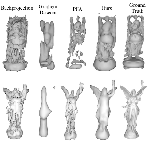
Figure 9. Reconstructions from simulated measurements using backprojection, gradient descent, the polar formatting algorithm (PFA), and our method. Compared to other methods, our reconstructions more accurately match the ground truth geometry.

Meanwhile, to quantitatively evaluate each method, we use two 3D metrics (Chamfer (Borgefors, 1986) distance, intersection-over-union (IOU)) and two image metrics (PSNR, LPIPS (Zhang et al., 2018a)) for selected viewpoints of the 3D volume. The 3D metrics capture the entire point cloud reconstruction performance, while the 2D image metrics help capture the perceptual quality of the shape from the rendered viewpoints. We compute points for the 3D metrics by exporting each method’s predicted point cloud to a mesh. As the point cloud threshold (i.e., points ¡ threshold = 0) influences the predicted mesh, we sweep over possible thresholds and choose the threshold that maximizes the performance of each method. The Chamfer distance is calculated based on a point cloud sampled from the reconstructed mesh surface, while IOU is calculated using a voxel representation of the mesh. We compute image metrics on rendered depth-images of the predicted and ground truth mesh at 10 azimuth angles. We use the depth images as these are independent on illumination and rely solely on the the object’s reconstructed geometry.

Table 2. Simulation results showing the average quantitative metrics for Backprojection (BP), Gradient descent (GD), the Polar formatting algorithm (PFA), and our reconstructions of 8 different meshes.

Metric	Chamfer $\downarrow$	IOU $\uparrow$	LPIPS $\downarrow$	PSNR $\uparrow$	MSE $\downarrow$
BP	1.36E-04	0.2928	0.1215	15.783	5.55E-03
GD	2.21E-04	0.4309	0.1236	15.117	6.13E-03
PFA	2.13E-04	0.3586	0.1238	15.048	6.64E-03
Ours	1.12E-04	0.5194	0.0988	17.918	3.99E-03

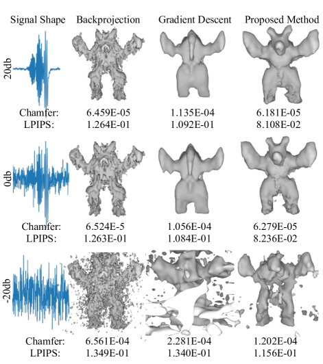
Figure 10. Simulation results using a $\Delta f=20$ kHz LFM showing the reconstructed meshes of an armadillo object at three noise levels. Our method performs decently well even at -20 dB signal-to-noise-ratio.

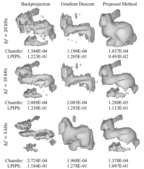
Figure 11. Simulation results using LFMs with different bandwidths $\Delta f$ to measure a bunny. As expected, the performance of all methods degrades at lower bandwidths, but our proposed method better preserves the object geometry.

8. Experimental Results

We validate our method on simulated data and two real-data sources. Section 8.1 presents our simulation results, where we test our method against baselines while varying experiment noise and bandwidths. Section 8.2 presents our first real-data source, AirSAS, where we test our method under varying measurement trajectories, bandwidths, and ablations. Finally, Section 8.3 presents our other real-data source, measurements captured of the Foster Joseph Sayers Reservoir, Pennsylvania using SVSS. Our SVSS results validate our method’s applicability to underwater environments and bistatic transducer arrays.

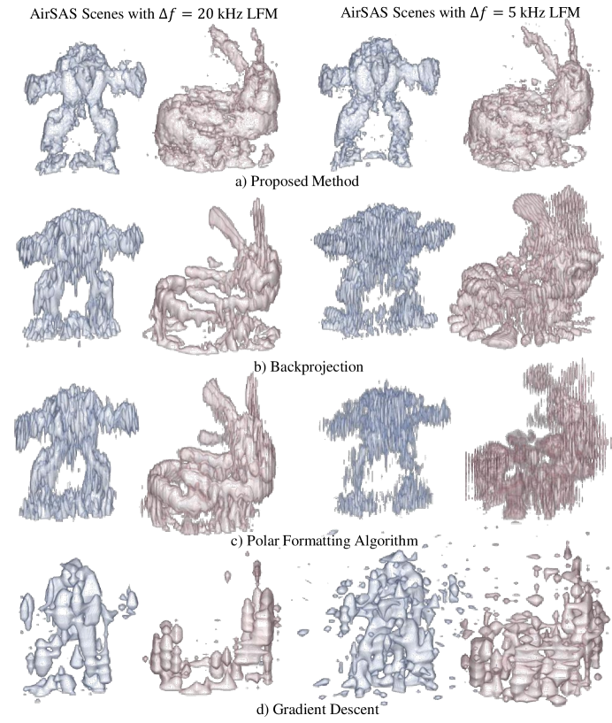
Figure 12. Reconstructions of AirSAS data captured with relatively high ($\Delta f=20$ kHz) and low ($\Delta f=5$ kHz) bandwidth LFMs. Our method demonstrates more consistent performance across waveform bandwidth compared to backprojection, the polar formatting algorithm, and gradient descent.

8.1. Simulation Results

Effectiveness of proposed method

We compare our proposed method against backprojection, the polar formatting algorithm, and gradient descent on simulated scenes measured with an LFM ($f_{c}=20$ kHz and $\Delta f=20$ kHz) at an SNR of $20$ dB. Table 2 presents quantitative metrics averaged over reconstructions from 8 different objects. Considering the PSNR metric, our approach offers $2$ dB improvement over other methods.

Figure 9 shows reconstructions of two objects used to compute the average in Table 2. In general, our method more accurately matches the ground truth geometry, especially occlusions in the mesh. We note that our method does lose some high-frequency details. We show reconstructions for all 8 meshes in the supplemental material.

Effects of noise:

In Fig. 10, we show armadillo reconstructions from each method at three SNR levels and measured using a $\Delta f=20$ kHz LFM. The bottom row of the figure shows an example waveform to highlight the challenge of reconstructing the scene under poor SNR conditions. As expected, the performance of each method tends to degrade as SNR decreases. Our method tends to outperform both competing methods at each noise level. We observe that the gradient descent method fails to recover higher frequency details on the object. There also seems to be a saturation level where 20 dB is not that much improved over 0 dB for all methods.

Effects of bandwidth:

Fig. 11 shows our next experiment, where a bunny object is simulated using three LFM bandwidths, $\Delta f=5kHz$, $\Delta f=10kHz$, and $\Delta f=20kHz$. As expected, the performance of all methods degrades at lower bandwidths, but we observe that our method tends to preserve the shape of spatial features more accurately compared to backprojection and gradient descent. This observation is reflected in the quantitative results, where our reconstructions generally report superior metrics.

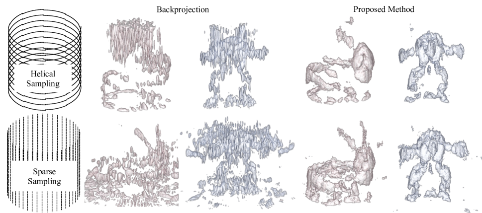
Figure 13. Helical and sparse view reconstructions of AirSAS measurements from $\Delta f=20$ kHz AirSAS bunny and armadillo. Our method can recover scene geometry while attenuating the undesirable image artifacts that plague backprojection in undersampled regimes.

8.2. AirSAS Reconstructions

Main results:

We reconstruct a 3D printed bunny and armadillo that were measured with an LFM of center frequency $f_{c}=20$kHz at bandwidths $\Delta f=20$ kHz and $\Delta f=5$ kHz. Fig. 12 shows the results of our method, backprojection, the polar formatting algorithm and gradient descent. First, we note that reconstruction quality decreases across all methods as the bandwidth decreases. However, the quality of our method is notably more consistent across the two bandwidth values, which conforms to our simulated results presented earlier. In the lower bandwidth case, our method produces notably more detailed and artifact-free reconstructions compared to the other methods. This is partially due to the fact that our pulse deconvolution performs similarly across both bandwidths, which is not the case for backprojection since it uses matched filtered waveforms. Additionally, neural backprojection helps overcome structural errors present in backprojection and PFA, such as the bunny’s concave head at the $20$ kHz bandwidth. We observe that the gradient descent method’s reconstruction is noisier and less accurate than ours, highlighting the importance of using an INR in neural backprojection.

Undersampling:

In real-world SAS applications, it is difficult to obtain multiple looks at an object from a dense collection of viewpoints. Thus we compare the performance of our method to backprojection in helical and sparse sampling schemes, as shown in Fig. 13. In both the helical and sparse sampling cases, we are using only approximately $10\%$ of the measurements required to be fully sampled in the traditional sense. Helical sampling is missing many vertical samples, and therefore induces vertical streaking artifacts in the backprojection results, as discussed in other works (Marston and Kennedy, 2016). While our method’s reconstruction is not perfect in this case, we highlight the fact that it contains fewer vertical streaking artifacts when compared to backprojection.

Sparse view sampling is common in computed-tomography literature, and is known to induce radial streaking artifacts in imagery due to the missing angles (Bian et al., 2010). As shown in the bottom row of Fig. 13, our method does remarkably well in this case, reconstructing a scene that is comparable to one obtained with fully sampled measurements. The notably superior performance of our method can potentially be attributed to our sparsity and smoothness priors, and also aligns with previous works that demonstrate the utility of INRs in limited data reconstruction problems (Rückert et al., 2022; Reed et al., 2021b; Sun et al., 2022).

Ablation studies:

Our ablations investigate various design choices in our pipeline. First, we perform an experiment to highlight the synergistic importance of both pulse deconvolution and neural backprojection in our method. In Fig. 14, we show an armadillo reconstruction using (1) matched-filtering and time-domain backprojection, (2) using matched-filtering and neural backprojection, (3) pulse deconvolution and time-domain backprojection, and (4) pulse deconvolution and neural backprojection (proposed approach). Clearly, both steps of our method are important for maximizing reconstruction quality. We observe that using match filtered waveforms with neural backprojection gives perhaps a slightly more accurate geometry, but is extremely noisy due to the limited range compression abilities of match-filtering. On the other hand, using our pulse deconvolved waveforms with traditional backprojection yields a smoother reconstruction than the traditional pipeline, but contains streaking artifacts common in backprojection algorithms.

Fig. 15 demonstrates the importance of our Lambertian scattering model by visualizing the normals computed by Eq.  (23). The reconstruction without the Lambertian model is noisier and sparser as the network struggles to reconstruct a scene consistent with given measurements since the 3D printed object is roughly diffuse in acoustic scattering. The normals also appear almost random without a Lambertian model, as the network was not constrained to output consistent surfaces.

Fig. 16 ablates the ability of our forward model to handle occlusion by setting $\zeta=0$ in the transmission probability calculation of Eq. 20. Without occlusion, neural backprojection fails to capture sharp outlines of the object’s geometry. As occlusion was a factor during the capture of the real-data, these artifacts are expected — the network predicts erroneous features since the forward model is unable to account for occlusion.

In the supplemental material, we also ablate for coherent versus incoherent SAS reconstruction as well as the effect of scene priors (e.g., sparsity) on reconstructions.

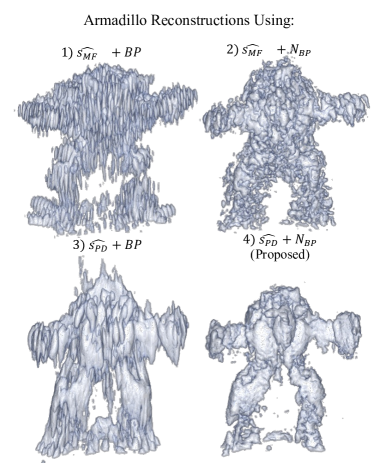
Figure 14. Ablating pulse deconvolution and neural backprojection using AirSAS $\Delta f=5$ kHz armadillo measurements. The top left (1) shows the traditional reconstruction pipeline that uses matched filtered waveforms as input to backprojection. The top right (2) shows using the matched filtered waveforms as input to neural backprojection. The bottom left (3) shows using the pulse deconvolved measurements as input to backprojection. The bottom right (4) is our proposed method and uses pulse deconvolution as input to neural backprojection. We observe that pulse deconvolution helps attenuate high-frequency surface noise, while neural backprojection aids in reconstructing accurate geometric features. Both pulse deconvolution and neural backprojection are important for maximizing reconstruction performance.

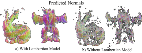
Figure 15. AirSAS reconstructions of scenes measured with a $\Delta f=20$ kHz LFM weighted by the 3D predicted normals encoded using the RGB channels. Left (a) shows reconstructions using the Lambertian model and right (b) shows reconstructions without using the Lambertian model. Using the Lambertian model yields better reconstructions and normal predictions since it enables the model to account for incidence angle.

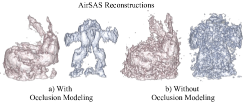
Figure 16. AirSAS reconstructions of scenes measured with a $\Delta f=20$ kHz LFM (a) with occlusion modeling and (b) without occlusion modeling. We turn off occlusion by setting $\zeta=0$ in the transmission probability of Eq. 20. Occlusion modeling is important for our method to obtain accurate reconstructions.

8.3. SVSS Reconstructions

Migrating from an in-lab to an in-water SAS deployed in the field brings a new set of challenges. First, the SVSS uses a more complicated sonar array that consists of five transmitters and eighty receivers, each with overlapping beamwidth that should be considered for accurate reconstructions.

Additionally, the energy backscattered from the lakebed is relatively strong compared to the targets. As such, we observe that a naive application of our deconvolution method using sparsity regularization tends to deconvolve returns from the lakebed and set the significantly smaller energy from the target close to zero. Using these measurements with neural backprojection yields subpar results since the objective function is mainly concerned with reconstructing the background. We address this issue by dynamic-range compressing our deconvolved measurements before passing them to the network — while this step amplifies noise, we find that that it makes the energy from the target strong enough for quality reconstructions. In particular, we dynamic-range compress measurements using $\mathbf{s}_{\text{PD}}^{\text{drc}}=\text{sign}(\mathbf{s}_{\text{PD}})|\mathbf{s}_{\text{PD}}|^{\kappa}$ where $\kappa\rightarrow 0$ increases the compression rate and $\text{sgn}(\cdot)$ returns the sign of the argument.

In Fig. 17, we show reconstructions of three targets of interest along an SVSS track. Note that we show a 2D maximum intensity projection (MIP) of an entire track in Fig. 1. Overall, our reconstructions appear sharper and with flatter side-profiles, because we better compress the waveforms during pulse deconvolution. In some cases, the object geometry appears more well-defined using our method, for example along the square cutouts in the cinder block. We also measure quantitative dimensions of the reconstructed cinder blocks (see supplemental material), and find that our method and backprojection are roughly equivalent in estimating metric lengths.

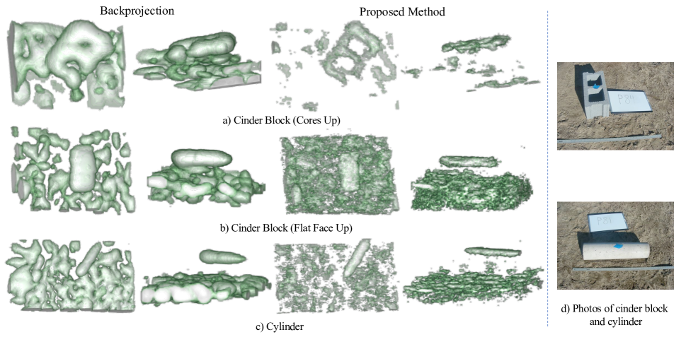
Figure 17. Two views of reconstructions with backprojection (left) and our proposed method (right) using in-water SAS data captured with SVSS. Our method recovers sharper object geometries, for example around the cinder block cores. Objects appear flatter in our reconstructions because of our pulse deconvolution step compressing measurements more than matched filtering. SVSS hardware photos courtesy of (Brown et al., 2021).

9. Discussion

We design an analysis-by-synthesis optimization for reconstructing SAS scenes, which yields several advantages to traditional approaches, including the ability to incorporate scene priors. We demonstrate the usefulness of this ability in Fig. 13, where we achieve far better reconstructions in the undersampled regimes of helical and sparse-view collection geometries. Additionally, our choice of a differentiable forward model influences image formation in interesting ways. For example, our inclusion of the Lambertian scattering model drastically improves our reconstructions, as shown in Fig. 15. These scattering constraints are easier to implement in our framework than with backprojection. We believe this work provides a promising avenue for future investigations into additional physics-based scattering models that enhance SAS reconstruction accuracy.

While existing acoustic renderers for simulating SAS measurements exist, we highlight the challenges of designing an efficient differentiable forward model for SAS compatible with analysis-by-synthesis optimization. In particular, we discuss the burdensome sampling requirements for integrating spherically propagating acoustic sources. We addressed this challenge in two ways. First, we proposed a pulse deconvolution step that yields waveforms with energy distributed among sparse time bins. In Section 6.1 (and derived in the supplemental material), we show that synthesis of each of these time bins equates to integrating the scene points that lie on the surfaces of ellipsoids. Second, we implement importance sampling in range and direction, and compute return rays only at the expected depth to make our optimization tractable for our 3D reconstructions.

The performance of our method contrasts with backprojection’s in meaningful ways. First, our method is less sensitive to transmit waveform bandwidth as shown in Fig. 12 when comparing the $\Delta f=20$ kHz and $\Delta f=5$ kHz reconstructions. As bandwidth is expensive (i.e., expensive transducers), these results demonstrate the potential for high-quality SAS imaging with inexpensive hardware. Second, our method typically recovers more accurate 3D shape details than backprojection. This is due to our pulse deconvolution step compressing the waveforms for accurate localization, and properly modeling occlusion, surface normals, and Lambertian scattering in our forward model.

9.1. Limitations and Future Work

There are disadvantages to analysis-by-synthesis frameworks applied to SAS reconstruction. First, our optimization is significantly slower than backprojection. Our reconstructions take up to 1-2 hours to complete, whereas backprojection can reconstruct scenes in minutes. Practically this implies a trade-off for the choice of reconstruction: backprojection may be most useful when surveying large underwater regions, whereas our method can be applied to enhance visual details to regions of interest identified in the backprojected imagery.

The second disadvantage of analysis-by-synthesis is that our reconstruction quality is limited by the accuracy of our forward model. Using a neural network in our pipeline can help compensate for forward model inaccuracies (Xie et al., 2022; Lucas et al., 2018), but this is true only to an extent. We observe that our model falls short of reconstructing effects ignored by our forward model, such as elastic scattering. Elastic scattering describes the phenomena where an insonified target stores then radiates acoustic energy (Al Mursaline et al., 2021). Elastic scattered energy can be seen as non-zero energy that appears to radiate downward from the cylinder approximately centered on the backprojected 3D reconstruction slice in Fig. 1. The presence of this energy is useful for target classification and detection (Brown et al., 2019b). While our proposed method predicts sharper object boundaries, this energy is notably absent in our reconstruction. This makes sense since our forward model has no mechanism to handle non-linear acoustics. An interesting future direction is to incorporate physics-based models that handle non-linear acoustics in our formulation.

There are interesting directions for future work related to accounting for uncertainty in our forward model. First, future work may find our method useful for solving joint unknown problems. For example, there is typically uncertainty in the SAS platform’s position with respect to the scene (Hayes and Gough, 2009). Future work may investigate using our analysis-by-synthesis framework to jointly solve for the platform position and the scene. Second, surrogate modeling may be useful for approximating inefficient and non-differentiable forward models with neural networks (Sun and Wang, 2019).

We now address some limitations with our pulse deconvolution step. In Fig. 14, we demonstrate the importance of this step, as using the matched filtered waveforms as input to neural backprojection drastically underperforms using the deconvolved pulse waveforms. However, deconvolution is an ill-posed inverse problem that is sensitive to noise, making the performance of this step depend on sparsity and smoothness hyperparameters. Thus, pulse deconvolution requires user input to select hyperparameters that maximize deconvolution performance. Future work may seek ways to robustly deconvolve the waveforms that minimize the need for hyperparameter tuning.

Finally, we mention that our deconvolution method and subsequent neural backprojection are done at the carrier frequency $f_{c}$, rather than at the baseband spectrum. Since we are operating at a relatively low carrier frequency ($f_{c}=20$ and $f_{c}=27.5$ kHz for AirSAS and SVSS, respectively), relative to our sampling rate $F_{s}=100$ kHZ, this is a non-issue. However, adapting this method to radar or even higher frequency SAS may require adapting the method to baseband signals. Empirically, we observed that trivially adapting our method to basebanded measurements results in worse reconstructions and therefore, it requires further investigation.

9.2. Conclusion

This work presents a reconstruction technique for SAS that we show outperforms traditional image formation in a number of settings. Importantly, we demonstrate that the method scales to in-water SAS data captured from field surveys. We believe this work to be an important step in advancing SAS imaging since it provides a framework for incorporating physics-based knowledge and custom priors into SAS image formation. More broadly, as this work demonstrates an impactful application of neural rendering for SAS, we believe it opens new possibilities for other synthetic aperture and coherent imaging fields like radar and ultrasound.

- (1)
- Ahn et al. (2019) Byeongjoo Ahn, Akshat Dave, Ashok Veeraraghavan, Ioannis Gkioulekas, and Aswin C Sankaranarayanan. 2019. Convolutional approximations to the general non-line-of-sight imaging operator. In Proceedings of the IEEE/CVF International Conference on Computer Vision. 7889–7899.
- Al Mursaline et al. (2021) Miad Al Mursaline, Timothy K Stanton, Andone C Lavery, and Erin M Fischell. 2021. Acoustic scattering by elastic cylinders: Practical sonar effects. The Journal of the Acoustical Society of America 150, 4 (2021), A327–A327.
- Arellano et al. (2017) Victor Arellano, Diego Gutierrez, and Adrian Jarabo. 2017. Fast back-projection for non-line of sight reconstruction. In ACM SIGGRAPH 2017 Posters. 1–2.
- Attal et al. (2021) Benjamin Attal, Eliot Laidlaw, Aaron Gokaslan, Changil Kim, Christian Richardt, James Tompkin, and Matthew O’Toole. 2021. TöRF: Time-of-Flight Radiance Fields for Dynamic Scene View Synthesis. Advances in Neural Information Processing Systems 34 (2021).
- Bamler (1992) Richard Bamler. 1992. A comparison of range-Doppler and wavenumber domain SAR focusing algorithms. IEEE Transactions on Geoscience and Remote Sensing 30, 4 (1992), 706–713.
- Bellettini and Pinto (2008) Andrea Bellettini and Marc Pinto. 2008. Design and experimental results of a 300-kHz synthetic aperture sonar optimized for shallow-water operations. IEEE Journal of Oceanic Engineering 34, 3 (2008), 285–293.
- Bertero et al. (2021) Mario Bertero, Patrizia Boccacci, and Christine De Mol. 2021. Introduction to inverse problems in imaging. CRC Press.
- Bian et al. (2010) Junguo Bian, Jeffrey H Siewerdsen, Xiao Han, Emil Y Sidky, Jerry L Prince, Charles A Pelizzari, and Xiaochuan Pan. 2010. Evaluation of sparse-view reconstruction from flat-panel-detector cone-beam CT. Physics in Medicine & Biology 55, 22 (2010), 6575.
- Blanford et al. (2022) Thomas E Blanford, Luke Garrett, J Daniel Park, and Daniel C Brown. 2022. Leveraging audio hardware for underwater acoustics experiments. In Proceedings of Meetings on Acoustics 182ASA, Vol. 46. Acoustical Society of America, 030002.
- Blanford et al. (2019) Thomas E. Blanford, John D. McKay, Daniel C. Brown, Joonho D. Park, and Shawn F. Johnson. 2019. Development of an in-air circular synthetic aperture sonar system as an educational tool. 177th Meeting of the Acoustical Society of America 36, 070002. https://doi.org/10.1121/2.0001025
- Borgefors (1986) Gunilla Borgefors. 1986. Distance transformations in digital images. Computer Vision, Graphics, and Image Processing 34, 3 (1986), 344–371.
- Bouman (2022) Charles A Bouman. 2022. Foundations of Computational Imaging: A Model-Based Approach. SIAM.
- Bracewell (1986) Ronald Newbold Bracewell. 1986. The Fourier transform and its applications. McGraw-Hill New York.
- Brown (2017) Daniel C Brown. 2017. Modeling and measurement of spatial coherence for normal incidence seafloor scattering. Ph. D. Dissertation. The Pennsylvania State University.
- Brown et al. (2019a) Daniel C Brown, Isaac D Gerg, and Thomas E Blanford. 2019a. Interpolation kernels for synthetic aperture sonar along-track motion estimation. IEEE Journal of Oceanic Engineering 45, 4 (2019), 1497–1505.
- Brown et al. (2021) Daniel C Brown, Shawn Johnson, Caleb Brownstead, Joeseph Calantoni, and Gene Fabian. 2021. Sediment Volume Search Sonar Development. Technical Report. https://serdp-estcp.org/projects/details/97e4a43c-bb65-432d-94ba-6aaff361571a
- Brown et al. (2019b) Daniel C Brown, Shawn F Johnson, Isaac D Gerg, and Cale F Brownstead. 2019b. Simulation and testing results for a sub-bottom ieee. In Proceedings of Meetings on Acoustics 177ASA, Vol. 36. Acoustical Society of America, 070001.
- Brown et al. (2017) Daniel C Brown, Shawn F Johnson, and Derek R Olson. 2017. A point-based scattering model for the incoherent component of the scattered field. The Journal of the Acoustical Society of America 141, 3 (2017), EL210–EL215.
- Callenberg et al. (2021) Clara Callenberg, Zheng Shi, Felix Heide, and Matthias B Hullin. 2021. Low-cost SPAD sensing for non-line-of-sight tracking, material classification and depth imaging. ACM Transactions on Graphics (TOG) 40, 4 (2021), 1–12.
- Callow (2003) Hayden J Callow. 2003. Signal Processing for Synthetic Aperture Sonar Image Enhancement. Ph. D. Dissertation. University of Canterbury.
- Callow et al. (2006) Hayden J Callow, Roy E Hansen, and TO Saebo. 2006. Effect of approximations in fast factorized backprojection in synthetic aperture imaging of spot regions. In OCEANS 2006. IEEE, 1–6.
- Callow et al. (2009) Hayden J Callow, Michael P Hayes, and Peter T Gough. 2009. Motion-compensation improvement for widebeam, multiple-receiver SAS systems. IEEE Journal of Oceanic Engineering 34, 3 (2009), 262–268.
- Cao et al. (2016) Chunxiao Cao, Zhong Ren, Carl Schissler, Dinesh Manocha, and Kun Zhou. 2016. Interactive sound propagation with bidirectional path tracing. ACM Transactions on Graphics (TOG) 35, 6 (2016), 1–11.
- Cao et al. (2019) Yuan Cao, Zhiying Fang, Yue Wu, Ding-Xuan Zhou, and Quanquan Gu. 2019. Towards understanding the spectral bias of deep learning. arXiv preprint arXiv:1912.01198 (2019).
- Chadwick et al. (2009) Jeffrey N Chadwick, Steven S An, and Doug L James. 2009. Harmonic shells: a practical nonlinear sound model for near-rigid thin shells. ACM Transactions on Graphics 28, 5 (2009), 1–119.
- Chadwick and James (2011) Jeffrey N Chadwick and Doug L James. 2011. Animating fire with sound. ACM Transactions on Graphics (TOG) 30, 4 (2011), 1–8.
- Chaillan et al. (2007) Fabien Chaillan, Christophe Fraschini, and Philippe Courmontagne. 2007. Speckle noise reduction in SAS imagery. Signal Processing 87, 4 (2007), 762–781.
- Chaitanya et al. (2020) Chakravarty R. Alla Chaitanya, Nikunj Raghuvanshi, Keith W. Godin, Zechen Zhang, Derek Nowrouzezahrai, and John M. Snyder. 2020. Directional Sources and Listeners in Interactive Sound Propagation Using Reciprocal Wave Field Coding. ACM Trans. Graph. 39, 4, Article 44 (7 2020), 14 pages. https://doi.org/10.1145/3386569.3392459
- Chandran and Jayasuriya (2019) Sreenithy Chandran and Suren Jayasuriya. 2019. Adaptive Lighting for Data-Driven Non-Line-of-Sight 3D Localization and Object Identification. In 30th British Machine Vision Conference 2019, BMVC 2019, Cardiff, UK, September 9-12, 2019. BMVA Press, 155. https://bmvc2019.org/wp-content/uploads/papers/0723-paper.pdf
- Chen et al. (2019) Wenzheng Chen, Simon Daneau, Fahim Mannan, and Felix Heide. 2019. Steady-state non-line-of-sight imaging. In Proceedings of the IEEE/CVF Conference on Computer Vision and Pattern Recognition. 6790–6799.
- Cook (2007) Daniel A Cook. 2007. Synthetic aperture sonar motion estimation and compensation. Ph. D. Dissertation. Georgia Institute of Technology.
- Cook and Brown (2008) Daniel A Cook and Daniel C Brown. 2008. Analysis of phase error effects on stripmap SAS. IEEE Journal of Oceanic Engineering 34, 3 (2008), 250–261.
- Cowen et al. (2021) Benjamin Cowen, J Daniel Park, Thomas E Blanford, Geoff Goehle, and Daniel C Brown. 2021. AirSAS: Controlled Dataset Generation for Physics-Informed Machine Learning. In NeurIPS Data-Centric AI Workshop.
- de Heering et al. (1994) Philippe de Heering, Klaus Uwe Simmer, Ezackiel Ochieng-Ogolla, and Alexander Wasiljeff. 1994. A Deconvolution Algorithm for Broadband Synthetic Aperture Data Processing. IEEE Journal of Oceanic Engineering 19 (1994), 73–83. Issue 1. https://doi.org/10.1109/48.289452
- Eaves and Reedy (2012) Jerry Eaves and Edward Reedy. 2012. Principles of modern radar. Springer Science & Business Media.
- Ferguson and Wyber (2005) Brian G Ferguson and Ron J Wyber. 2005. Application of acoustic reflection tomography to sonar imaging. The Journal of the Acoustical Society of America 117, 5 (2005), 2915–2928.
- Ferguson and Wyber (2009) Brian G Ferguson and Ron J Wyber. 2009. Generalized framework for real aperture, synthetic aperture, and tomographic sonar imaging. IEEE Journal of Oceanic Engineering 34, 3 (2009), 225–238.
- Fienup (2000) JR Fienup. 2000. Synthetic-aperture radar autofocus by maximizing sharpness. Optics letters 25, 4 (2000), 221–223.
- Fortune et al. (2001) SA Fortune, MP Hayes, and PT Gough. 2001. Statistical autofocus of synthetic aperture sonar images using image contrast optimisation. In MTS/IEEE Oceans 2001. An Ocean Odyssey. Conference Proceedings (IEEE Cat. No. 01CH37295), Vol. 1. IEEE, 163–169.
- Fridovich-Keil and Yu et al. (2022) Fridovich-Keil and Yu, Matthew Tancik, Qinhong Chen, Benjamin Recht, and Angjoo Kanazawa. 2022. Plenoxels: Radiance Fields without Neural Networks. In CVPR.
- Gerg and Monga (2020) Isaac Gerg and Vishal Monga. 2020. Deep Autofocus for Synthetic Aperture Sonar. arXiv preprint arXiv:2010.15687 (2020).
- Gerg et al. (2020) Isaac D Gerg, Daniel C Brown, Stephen G Wagner, Daniel Cook, Brian N O’Donnell, Thomas Benson, and Thomas C Montgomery. 2020. GPU Acceleration for Synthetic Aperture Sonar Image Reconstruction. In Global Oceans 2020: Singapore–US Gulf Coast. IEEE, 1–9.
- Gerg and Monga (2021) Isaac D Gerg and Vishal Monga. 2021. Real-Time, Deep Synthetic Aperture Sonar (SAS) Autofocus. In 2021 IEEE International Geoscience and Remote Sensing Symposium IGARSS. IEEE, 8684–8687.
- Goehle et al. (2022) Geoff Goehle, Benjamin Cowen, Thomas E Blanford, J Daniel Park, and Daniel C Brown. 2022. Approximate extraction of late-time returns via morphological component analysis. arXiv preprint arXiv:2208.06056 (2022).
- Gough and Hawkins (1997a) Peter T Gough and David W Hawkins. 1997a. Imaging algorithms for a strip-map synthetic aperture sonar: Minimizing the effects of aperture errors and aperture undersampling. IEEE Journal of Oceanic Engineering 22, 1 (1997), 27–39.
- Gough and Hawkins (1997b) Peter T Gough and David W Hawkins. 1997b. Unified framework for modern synthetic aperture imaging algorithms. International Journal of Imaging Systems and Technology 8, 4 (1997), 343–358.
- Griffiths et al. (1997) HD Griffiths, TA Rafik, Z Meng, CFN Cowan, H Shafeeu, and DK Anthony. 1997. Interferometric synthetic aperture sonar for high-resolution 3-D mapping of the seabed. IEE Proceedings-Radar, Sonar and Navigation 144, 2 (1997), 96–103.
- Gul et al. (2017) Sana Gul, S Sajjad Haider Zaidi, Rehan Khan, and Ammar Banduk Wala. 2017. Underwater acoustic channel modeling using BELLHOP ray tracing method. In 2017 14th International Bhurban Conference on Applied Sciences and Technology (IBCAST). IEEE, 665–670.
- Hamilton et al. (2017) Brian Hamilton, Stefan Bilbao, Brian Hamilton, and Stefan Bilbao. 2017. FDTD Methods for 3-D Room Acoustics Simulation With High-Order Accuracy in Space and Time. IEEE/ACM Trans. Audio, Speech and Lang. Proc. 25, 11 (11 2017), 2112–2124. https://doi.org/10.1109/TASLP.2017.2744799
- Hansen et al. (2011) Roy Edgar Hansen, Hayden John Callow, Torstein Olsmo Sabo, and Stig Asle Vaksvik Synnes. 2011. Challenges in seafloor imaging and mapping with synthetic aperture sonar. IEEE Transactions on Geoscience and Remote Sensing 49, 10 (2011), 3677–3687.
- Hansen et al. (2003) Roy Edgar Hansen, Torstien Olsom Saebo, Kenneth Gade, and Sean Chapman. 2003. Signal processing for AUV based interferometric synthetic aperture sonar. IEEE Oceans 2003 5 (2003), 2438–2444.
- Harrison (2019) Lee Andrew Andy Harrison. 2019. Introduction to Radar using Python and MATLAB. Artech House.
- Hawkins (1996) David William Hawkins. 1996. Synthetic aperture imaging algorithms: with application to wide bandwidth sonar. Ph. D. Dissertation. University of Canterbury.
- Hayes and Gough (1992) Michael P Hayes and Peter T Gough. 1992. Broad-band synthetic aperture sonar. IEEE Journal of Oceanic Engineering 17, 1 (1992), 80–94.
- Hayes and Gough (2009) Michael P Hayes and Peter T Gough. 2009. Synthetic aperture sonar: A review of current status. IEEE Journal of Oceanic Engineering 34, 3 (2009), 207–224.
- Heide et al. (2013) Felix Heide, Matthias B Hullin, James Gregson, and Wolfgang Heidrich. 2013. Low-budget transient imaging using photonic mixer devices. ACM Transactions on Graphics (ToG) 32, 4 (2013), 1–10.
- Iseringhausen and Hullin (2020) Julian Iseringhausen and Matthias B Hullin. 2020. Non-line-of-sight reconstruction using efficient transient rendering. ACM Transactions on Graphics (ToG) 39, 1 (2020), 1–14.
- Jensen et al. (2006) Jørgen Arendt Jensen, Svetoslav Ivanov Nikolov, Kim Løkke Gammelmark, and Morten Høgholm Pedersen. 2006. Synthetic aperture ultrasound imaging. Ultrasonics 44 (2006), e5–e15.
- Johnson and Brown (2018) Shawn F Johnson and Daniel C Brown. 2018. SAS simulations with procedural texture and the point-based sonar scattering model. In OCEANS 2018 MTS/IEEE Charleston. IEEE, 1–7.
- Kadambi et al. (2013) Achuta Kadambi, Refael Whyte, Ayush Bhandari, Lee Streeter, Christopher Barsi, Adrian Dorrington, and Ramesh Raskar. 2013. Coded time of flight cameras: sparse deconvolution to address multipath interference and recover time profiles. ACM Transactions on Graphics (ToG) 32, 6 (2013), 1–10.
- Kadambi et al. (2016) Achuta Kadambi, Hang Zhao, Boxin Shi, and Ramesh Raskar. 2016. Occluded imaging with time-of-flight sensors. ACM Transactions on Graphics (ToG) 35, 2 (2016), 1–12.
- Kaipio and Somersalo (2004) Jari P Kaipio and Erkki Somersalo. 2004. Computational and statistical methods for inverse problems. Applied Mathematical Sciences 160 (2004).
- Kim and Kim (2021) Juhyeon Kim and Young Min Kim. 2021. Fast and Lightweight Path Guiding Algorithm on GPU. In Pacific Graphics Short Papers, Posters, and Work-in-Progress Papers, Sung-Hee Lee, Stefanie Zollmann, Makoto Okabe, and Burkhard Wünsche (Eds.). The Eurographics Association. https://doi.org/10.2312/pg.20211379
- Kingma and Ba (2014) Diederik P Kingma and Jimmy Ba. 2014. Adam: A method for stochastic optimization. arXiv preprint arXiv:1412.6980 (2014).
- Lambert (1760) Johann Heinrich Lambert. 1760. Photometria sive de mensura et gradibus luminis, colorum et umbrae. sumptibus vidvae E. Klett, typis CP Detleffsen.
- Lannes et al. (1997) André Lannes, Eric Anterrieu, and Pierre Maréchal. 1997. Clean and wipe. Astronomy and Astrophysics Supplement Series 123, 1 (1997), 183–198.
- Levoy and Hanrahan (1996) Marc Levoy and Pat Hanrahan. 1996. Light field rendering. Proceedings of the 23rd Annual Conference on Computer Graphics and Interactive Techniques (1996), 31–42.
- Lindell et al. (2019a) David B Lindell, Gordon Wetzstein, and Vladlen Koltun. 2019a. Acoustic non-line-of-sight imaging. In Proceedings of the IEEE/CVF Conference on Computer Vision and Pattern Recognition. 6780–6789.
- Lindell et al. (2019b) David B Lindell, Gordon Wetzstein, and Matthew O’Toole. 2019b. Wave-based non-line-of-sight imaging using fast fk migration. ACM Transactions on Graphics (ToG) 38, 4 (2019), 1–13.
- Liu and Manocha (2020) Shiguang Liu and Dinesh Manocha. 2020. Sound synthesis, propagation, and rendering: a survey. arXiv preprint arXiv:2011.05538 (2020).
- Liu et al. (2019) Xiaochun Liu, Ibón Guillén, Marco La Manna, Ji Hyun Nam, Syed Azer Reza, Toan Huu Le, Adrian Jarabo, Diego Gutierrez, and Andreas Velten. 2019. Non-line-of-sight imaging using phasor-field virtual wave optics. Nature 572, 7771 (2019), 620–623.
- Lucas et al. (2018) Alice Lucas, Michael Iliadis, Rafael Molina, and Aggelos K Katsaggelos. 2018. Using deep neural networks for inverse problems in imaging: beyond analytical methods. IEEE Signal Processing Magazine 35, 1 (2018), 20–36.
- Mansour et al. (2018) Hassan Mansour, Dehong Liu, Ulugbek S. Kamilov, and Petros T. Boufounos. 2018. Sparse Blind Deconvolution for Distributed Radar Autofocus Imaging. (5 2018). http://arxiv.org/abs/1805.03269
- Marston and Kennedy (2016) Timothy M Marston and Jermaine L Kennedy. 2016. Volumetric acoustic imaging via circular multipass aperture synthesis. IEEE Journal of Oceanic Engineering 41, 4 (2016), 852–867.
- Marston et al. (2011) Timothy M Marston, Jermaine L Kennedy, and Philip L Marston. 2011. Coherent and semi-coherent processing of limited-aperture circular synthetic aperture (CSAS) data. In OCEANS’11 MTS/IEEE KONA. IEEE, 1–6.
- Marston et al. (2014) Timothy M Marston, Jermaine L Kennedy, and Philip L Marston. 2014. Autofocusing circular synthetic aperture sonar imagery using phase corrections modeled as generalized cones. The Journal of the Acoustical Society of America 136, 2 (2014), 614–622.
- Mildenhall et al. (2021) Ben Mildenhall, Pratul P Srinivasan, Matthew Tancik, Jonathan T Barron, Ravi Ramamoorthi, and Ren Ng. 2021. Nerf: Representing scenes as neural radiance fields for view synthesis. Commun. ACM 65, 1 (2021), 99–106.
- Müller et al. (2022) Thomas Müller, Alex Evans, Christoph Schied, and Alexander Keller. 2022. Instant Neural Graphics Primitives with a Multiresolution Hash Encoding. ACM Trans. Graph. 41, 4, Article 102 (July 2022), 15 pages. https://doi.org/10.1145/3528223.3530127
- Nadimi et al. (2021) Nahid Nadimi, Reza Javidan, and Kamran Layeghi. 2021. Efficient Detection of Underwater Natural Gas Pipeline Leak Based on Synthetic Aperture Sonar (SAS) Systems. Journal of Marine Science and Engineering 9, 11 (2021), 1273.
- O’Toole et al. (2017) Matthew O’Toole, Felix Heide, David B Lindell, Kai Zang, Steven Diamond, and Gordon Wetzstein. 2017. Reconstructing transient images from single-photon sensors. In Proceedings of the IEEE conference on computer vision and pattern recognition. 1539–1547.
- Pailhas et al. (2017) Yan Pailhas, Yvan Petillot, and Bernard Mulgrew. 2017. Increasing circular synthetic aperture sonar resolution via adapted wave atoms deconvolution. The Journal of the Acoustical Society of America 141 (4 2017), 2623–2632. Issue 4. https://doi.org/10.1121/1.4979807
- Park et al. (2020) J Daniel Park, Thomas E Blanford, Daniel C Brown, and Daniel Plotnick. 2020. Alternative representations and object classification of circular synthetic aperture in-air acoustic data. The Journal of the Acoustical Society of America 148, 4 (2020), 2661–2661.
- Pediredla et al. (2019) Adithya Pediredla, Ashok Veeraraghavan, and Ioannis Gkioulekas. 2019. Ellipsoidal path connections for time-gated rendering. ACM Transactions on Graphics (TOG) 38, 4 (2019), 1–12.
- Pierce (1981) A. D. Pierce. 1981. Acoustics: An introduction to its physical principles and applications. (1981), 486–487.
- Piper et al. (2002) John E Piper, Kerry W Commander, Eric I Thorsos, and Kevin L Williams. 2002. Detection of buried targets using a synthetic aperture sonar. IEEE Journal of Oceanic Engineering 27, 3 (2002), 495–504.
- Plack et al. (2023) Markus Plack, Clara Callenberg, Monika Schneider, and Matthias B Hullin. 2023. Fast Differentiable Transient Rendering for Non-Line-of-Sight Reconstruction. In Proceedings of the IEEE/CVF Winter Conference on Applications of Computer Vision. 3067–3076.
- Plotnick et al. (2014) Daniel S Plotnick, Philip L Marston, and Timothy M Marston. 2014. Fast nearfield to farfield conversion algorithm for circular synthetic aperture sonar. The Journal of the Acoustical Society of America 136, 2 (2014), EL61–EL66.
- Poole et al. (2022) Ben Poole, Ajay Jain, Jonathan T. Barron, and Ben Mildenhall. 2022. DreamFusion: Text-to-3D using 2D Diffusion. arXiv (2022).
- Potokar et al. (2022) Easton Potokar, Spencer Ashford, Michael Kaess, and Joshua G Mangelson. 2022. HoloOcean: An underwater robotics simulator. In 2022 International Conference on Robotics and Automation (ICRA). IEEE, 3040–3046.
- Putney and Anderson (2005) Angela Putney and Richard H. Anderson. 2005. Reconstruction of under-sampled SAS data using the WIPE algorithm. Proceedings of MTS/IEEE OCEANS, 2005 2005, 111–118. https://doi.org/10.1109/OCEANS.2005.1639747
- Qadri et al. (2023) M. Qadri, M. Kaess, and I. Gkioulekas. 2023. Neural Implicit Surface Reconstruction using Imaging Sonar. In Proc. IEEE Intl. Conf. on Robotics and Automation, ICRA. London, UK. To appear.
- Raghuvanshi and Snyder (2014) Nikunj Raghuvanshi and John Snyder. 2014. Parametric Wave Field Coding for Precomputed Sound Propagation. ACM Trans. Graph. 33, 4, Article 38 (7 2014), 11 pages. https://doi.org/10.1145/2601097.2601184
- Raghuvanshi et al. (2010) Nikunj Raghuvanshi, John Snyder, Ravish Mehra, Ming Lin, and Naga Govindaraju. 2010. Precomputed Wave Simulation for Real-Time Sound Propagation of Dynamic Sources in Complex Scenes. ACM Trans. Graph. 29, 4, Article 68 (7 2010), 11 pages. https://doi.org/10.1145/1778765.1778805
- Ramamoorthi and Hanrahan (2001) Ravi Ramamoorthi and Pat Hanrahan. 2001. A signal-processing framework for inverse rendering. In Proceedings of the 28th Annual Conference on Computer Graphics and Interactive Techniques. 117–128.
- Reed et al. (2021a) Albert Reed, Thomas Blanford, Daniel C. Brown, and Suren Jayasuriya. 2021a. Implicit Neural Representations for Deconvolving SAS Images. In OCEANS 2021: San Diego – Porto. 1–7. https://doi.org/10.23919/OCEANS44145.2021.9705799
- Reed et al. (2022) Albert Reed, Thomas Blanford, Daniel C. Brown, and Suren Jayasuriya. 2022. SINR: Deconvolving Circular SAS Images Using Implicit Neural Representations. IEEE Journal of Selected Topics in Signal Processing (2022), 1–16. https://doi.org/10.1109/JSTSP.2022.3215849
- Reed et al. (2019) Albert Reed, Isaac D Gerg, John D McKay, Daniel C Brown, David P Williamsk, and Suren Jayasuriya. 2019. Coupling rendering and generative adversarial networks for artificial SAS image generation. In OCEANS 2019 MTS/IEEE SEATTLE. IEEE, 1–10.
- Reed et al. (2021b) Albert W. Reed, Hyojin Kim, Rushil Anirudh, K. Aditya Mohan, Kyle Champley, Jingu Kang, and Suren Jayasuriya. 2021b. Dynamic CT Reconstruction from Limited Views with Implicit Neural Representations and Parametric Motion Fields. 2021 IEEE/CVF International Conference on Computer Vision (ICCV) (2021), 2238–2248. https://doi.org/10.1109/ICCV48922.2021.00226
- Rückert et al. (2022) Darius Rückert, Yuanhao Wang, Rui Li, Ramzi Idoughi, and Wolfgang Heidrich. 2022. NeAT: Neural Adaptive Tomography. ACM Transactions on Graphics (2022).
- Sammelmann (2001) G.S. Sammelmann. 2001. Propagation and scattering in very shallow water. In MTS/IEEE Oceans 2001. An Ocean Odyssey. Conference Proceedings (IEEE Cat. No.01CH37295), Vol. 1. 337–344 vol.1. https://doi.org/10.1109/OCEANS.2001.968749
- Savioja and Svensson (2015) Lauri Savioja and U Peter Svensson. 2015. Overview of geometrical room acoustic modeling techniques. The Journal of the Acoustical Society of America 138, 2 (2015), 708–730.
- Schissler et al. (2014) Carl Schissler, Ravish Mehra, and Dinesh Manocha. 2014. High-Order Diffraction and Diffuse Reflections for Interactive Sound Propagation in Large Environments. ACM Trans. Graph. 33, 4, Article 39 (7 2014), 12 pages. https://doi.org/10.1145/2601097.2601216
- Schweickart et al. (2017) Eston Schweickart, Doug L James, and Steve Marschner. 2017. Animating elastic rods with sound. ACM Transactions on Graphics (TOG) 36, 4 (2017), 1–10.
- Shen et al. (2021) Siyuan Shen, Zi Wang, Ping Liu, Zhengqing Pan, Ruiqian Li, Tian Gao, Shiying Li, and Jingyi Yu. 2021. Non-line-of-Sight Imaging via Neural Transient Fields. IEEE Transactions on Pattern Analysis and Machine Intelligence (2021).
- Siltanen et al. (2007) Samuel Siltanen, Tapio Lokki, Sami Kiminki, and Lauri Savioja. 2007. The room acoustic rendering equation. The Journal of the Acoustical Society of America 122, 3 (2007), 1624–1635.
- Smith (1997) Steven W Smith. 1997. The scientist and engineer’s guide to digital signal processing. California Technical Pub. San Diego.
- Soumekh (1999) Mehrdad Soumekh. 1999. Synthetic aperture radar signal processing. Vol. 7. New York: Wiley.
- Sture et al. (2018) Øystein Sture, Martin Ludvigsen, Margrete S Scheide, and Terje Thorsnes. 2018. Recognition of cold-water corals in synthetic aperture sonar imagery. In 2018 IEEE/OES Autonomous Underwater Vehicle Workshop (AUV). IEEE, 1–6.
- Sun and Wang (2019) Gang Sun and Shuyue Wang. 2019. A review of the artificial neural network surrogate modeling in aerodynamic design. Proceedings of the Institution of Mechanical Engineers, Part G: Journal of Aerospace Engineering 233, 16 (2019), 5863–5872.
- Sun et al. (2022) Yu Sun, Jiaming Liu, Mingyang Xie, Brendt Wohlberg, and Ulugbek S Kamilov. 2022. Coil: Coordinate-based internal learning for imaging inverse problems. IEEE Transactions on Computational Imaging (2022).
- Velten et al. (2012) Andreas Velten, Thomas Willwacher, Otkrist Gupta, Ashok Veeraraghavan, Moungi G Bawendi, and Ramesh Raskar. 2012. Recovering three-dimensional shape around a corner using ultrafast time-of-flight imaging. Nature Communications 3, 1 (2012), 745.
- Wallis et al. (1989) J.W. Wallis, T.R. Miller, C.A. Lerner, and E.C. Kleerup. 1989. Three-Dimensional Display in Nuclear Medicine. IEEE Trans. Med. Imag. 8, 4 (Dec. 1989), 297–303. https://doi.org/10.1109/42.41482
- Wang et al. (2018) Jui-Hsien Wang, Ante Qu, Timothy R Langlois, and Doug L James. 2018. Toward wave-based sound synthesis for computer animation. ACM Trans. Graph. 37, 4 (2018), 109–1.
- Williams (2016) David P Williams. 2016. Underwater target classification in synthetic aperture sonar imagery using deep convolutional neural networks. In 2016 23rd International Conference on Pattern Recognition (ICPR). IEEE, 2497–2502.
- Woods (2020) Denton Woods. 2020. Ray-based methods in PC SWAT. The Journal of the Acoustical Society of America 148, 4 (2020), 2796–2796.
- Wu et al. (2021) Lifan Wu, Guangyan Cai, Ravi Ramamoorthi, and Shuang Zhao. 2021. Differentiable time-gated rendering. ACM Transactions on Graphics (TOG) 40, 6 (2021), 1–16.
- Xie et al. (2022) Yiheng Xie, Towaki Takikawa, Shunsuke Saito, Or Litany, Shiqin Yan, Numair Khan, Federico Tombari, James Tompkin, Vincent Sitzmann, and Srinath Sridhar. 2022. Neural fields in visual computing and beyond. In Computer Graphics Forum, Vol. 41. Wiley Online Library, 641–676.
- Yi et al. (2021) Shinyoung Yi, Donggun Kim, Kiseok Choi, Adrian Jarabo, Diego Gutierrez, and Min H Kim. 2021. Differentiable transient rendering. ACM Transactions on Graphics (TOG) 40, 6 (2021), 1–11.
- Yu et al. (2006) Lian Yu, Nicola Neretti, and Nathan Intrator. 2006. Multiple ping sonar accuracy improvement using robust motion estimation and ping fusion. The Journal of the Acoustical Society of America 119, 4 (2006), 2106–2113.
- Zang et al. (2021) Guangming Zang, Ramzi Idoughi, Rui Li, Peter Wonka, and Wolfgang Heidrich. 2021. IntraTomo: Self-supervised Learning-based Tomography via Sinogram Synthesis and Prediction. In Proceedings of the IEEE/CVF International Conference on Computer Vision. 1960–1970.
- Zhang et al. (2018a) Richard Zhang, Phillip Isola, Alexei A Efros, Eli Shechtman, and Oliver Wang. 2018a. The unreasonable effectiveness of deep features as a perceptual metric. In Proceedings of the IEEE Conference on Computer Vision and Pattern Recognition. 586–595.
- Zhang et al. (2021) Xiuming Zhang, Pratul P Srinivasan, Boyang Deng, Paul Debevec, William T Freeman, and Jonathan T Barron. 2021. Nerfactor: Neural factorization of shape and reflectance under an unknown illumination. ACM Transactions on Graphics (TOG) 40, 6 (2021), 1–18.
- Zhang et al. (2018b) Zechen Zhang, Nikunj Raghuvanshi, John Snyder, and Steve Marschner. 2018b. Ambient sound propagation. ACM Transactions on Graphics (TOG) 37, 6 (2018), 1–10.
- Zhang et al. (2019) Zechen Zhang, Nikunj Raghuvanshi, John Snyder, and Steve Marschner. 2019. Acoustic texture rendering for extended sources in complex scenes. ACM Transactions on Graphics (TOG) 38, 6 (2019), 1–9.
- Zheng and James (2010) Changxi Zheng and Doug L James. 2010. Rigid-body fracture sound with precomputed soundbanks. ACM SIGGRAPH 2010 papers (2010), 1–13.