Improving Spectrum-Based Localization of Multiple Faults by Iterative Test Suite Reduction

Abstract.

Spectrum-based fault localization (SBFL) works well for single-fault programs but its accuracy decays for increasing fault numbers. We present FLITSR (Fault Localization by Iterative Test Suite Reduction), a novel SBFL extension that improves the localization of a given base metric specifically in the presence of multiple faults. FLITSR iteratively selects reduced versions of the test suite that better localize the individual faults in the system. This allows it to identify and re-rank faults ranked too low by the base metric because they were masked by other program elements.

We evaluated FLITSR over method-level spectra from an existing large synthetic dataset comprising 75000 variants of 15 open-source projects with up to 32 injected faults, as well as method- and statement-level spectra from a new dataset with 326 true multi-fault versions from the Defects4J benchmark set containing up to 14 real faults. For all three spectrum types we consistently see substantial reductions of the average wasted efforts at different fault levels, of 30%-90% over the best base metric, and generally similarly large increases in precision and recall, albeit with larger variance across the underlying projects. For the method-level real faults, FLITSR also substantially outperforms GRACE, a state-of-the-art learning-based fault localizer.

1. Introduction

Debugging (i.e., finding and fixing bugs) contributes to a large part of the costs of the software development process (Vessey, 1985), and substantial efforts have been made to automate it (Wong et al., 2016; Zou et al., 2021). Debugging involves fault localization, fault understanding, and fault correction (Parnin and Orso, 2011); we focus on the first here. There are many approaches to automated fault localization, most notably learning-based (Lou et al., 2021; Li et al., 2019; Wong et al., 2012b), model-based (Wong et al., 2016; Mayer and Stumptner, 2008), and spectrum-based fault localization (SBFL) (de Souza et al., 2016; Jones et al., 2002; Abreu et al., 2006; Wong et al., 2014). SBFL is a lightweight and scalable approach that summarizes coverage information for each program element over a given test suite into a spectrum, and uses a given formula or metric to compute from the spectrum a suspiciousness score, which is seen as likelihood for elements to contain a fault.

SBFL has been widely studied, with a variety of different metrics and extensions suggested (see Section 6), and with successful applications to downstream tasks such as automated program repair (Debroy and Wong, 2010; Forrest et al., 2009; Nguyen et al., 2013). In several studies involving single-fault programs, users of SBFL tools were found to be more effective (i.e., found more bugs) (Gouveia et al., 2013; de Souza et al., 2022; Xia et al., 2016; Xie et al., 2016) and more efficient (i.e., found bugs faster) (Gouveia et al., 2013; de Souza et al., 2022; Horváth et al., 2020) than users without such tools. SBFL has been shown to perform well when there are only a few test failures related to a single fault (Heiden et al., 2019). However, its effectiveness degrades, in particular beyond the first fault, when there are multiple test failures related to multiple faults (DiGiuseppe and Jones, 2011). This multi-fault localization (MFL) problem naturally emerges in many situations, e.g., after testing by external QA, fuzzing campaigns, or field releases of new versions, or simply through the accumulation of unresolved issues.

Several approaches have been proposed to address the MFL problem (Zakari et al., 2020). The most widely used one is the one-bug-at-a-time (OBA) approach (Jones et al., 2002; Debroy and Wong, 2009; Wong et al., 2014, 2012a; Jones and Harrold, 2005), which iteratively finds and fixes the top-ranked faults. However, OBA is not realistic in practice, where bugs are fixed based on priorities other than their SBFL rank (e.g., system impact, time to fix, availability of developer responsible for the code, etc.). Alternatively, in the parallel debugging approach the spectrum is decomposed into several blocks or fault-focused clusters where failures caused by the same fault are grouped into the same cluster (Jones et al., 2007; Wong et al., 2012b; Gao and Wong, 2019; Steimann and Frenkel, 2012). However, due to fault interference and fault masking the decompositions are often imperfect (Hogerle et al., 2014), so that clusters again induce an MFL problem. True multiple-bug-at-a-time (MBA) approaches localize multiple faults in one run, without any changes to the target system. However, MBA has “enjoyed little attention” (Zakari et al., 2020), with only few approaches published (Abreu et al., 2011, 2009a; Zakari et al., 2018; Zheng et al., 2018). Most of these require exceedingly large runtimes due to their incorporation of various other technologies such as SAT solvers (Abreu et al., 2009a).

In this paper, we address this gap and present a novel, purely spectrum-based MBA approach called FLITSR (Fault Localization by Iterative Test Suite Reduction). It is based on the observation that in a ranking induced by an SBFL metric, the position of faulty elements is influenced by the density of failing tests executing each of these faults. Our key insight is that by removing from the test suite the failing tests executing the most suspicious element, we can increase the relative density of failing tests executing the remaining faulty elements, and so improve the ranks of these faults. We can thus use any SBFL metric in a feedback loop (alternating between localizing and recording the most suspicious element and removing its associated failing tests) in order to reduce the test suite in each iteration to localize the remaining faults more accurately. Through this process, FLITSR constructs a set of highly suspicious program elements called a basis, where the execution of each failing test in the test suite involves at least one basis element. The basis element(s) executed in this test can thus be seen as the cause of the test failure, and the constructed basis thus fully explains all test failures. FLITSR then computes a new ranking by shifting the basis elements towards the top, since it considers them as the elements most likely to contain a fault. For most program spectra, multiple bases exist; we exploit this in a variant of FLITSR called FLITSR*, which iteratively calculates the various bases, and ranks them in the order that they were found. This sequence of bases also gives us a sequence of natural cut-off points (i.e., the end of each basis in the ranking), where developers can choose to stop inspecting the ranking as further inspection yields diminishing returns. This is in line with how developers use SBFL tools (Parnin and Orso, 2011).

FLITSR is generic in the SBFL metric used and extends any metric’s induced localization to the MFL scenario, even if the given metric was originally developed for single faults. We experimentally evaluate FLITSR using eleven well-performing SBFL metrics including popular single-fault metrics (Jones et al., 2002; Abreu et al., 2006; Wong et al., 2014; Yoo, 2012; Wong et al., 2007; Naish et al., 2011), state-of-the-art multi-fault metrics (Hogerle et al., 2014; Abreu et al., 2009a, b; Neelofar et al., 2018), and learning-based metrics (Lou et al., 2021), and show that it unanimously improves on all base metrics, providing the best overall ranking using metrics that perform best in the single-fault case. This shows that FLITSR indeed successfully extends single-fault solutions to the multi-fault case.

The current evaluation of MFL techniques poses significant problems, due to the scarcity of suitable datasets with known fault locations. We first use an existing set of test coverage matrices (TCMs) (Hogerle et al., 2014; tcm, [n. d.]; Steimann et al., 2013) that has also been used in other projects (Steimann et al., 2013; Steimann and Frenkel, 2012; Sun and Podgurski, 2016), with up to $N_{f}=32$ injected faults. Here, the best FLITSR*-variant reduces the average wasted effort to the first resp. median fault by 20% resp. 40% ($N_{f}=4$) to 35% resp. 45% ($N_{f}=32$), compared to the best base metric, and increases precision by 60%, and recall by 40% to 75%.

We also contribute a new multi-fault dataset derived from the Defects4J dataset (Just et al., 2014a) of real bugs, and use it to evaluate FLITSR at the method and statement levels. This is the first large multi-fault dataset that contains only existing real faults. For this dataset, the results vary considerably between the individual projects, and in fact more than between method- and statement-level. For two projects (Chart and Lang), FLITSR yields substantial (30%-90%) method-level wasted effort reductions, and similar increases in recall (30%) and precision (20%-50%), and can pinpoint the top error in about half of the cases. For the remaining three projects, FLITSR* can improve on FLITSR, with improvements over the base metric for all measures in almost all cases. At the statement-level, the overall results are similar, but the improvements are relatively smaller, due to the larger sizes of the spectra. We finally show that FLITSR outperforms by a wide margin GRACE (Lou et al., 2021), a state-of-the-art learning-based method-level fault localizer.

In this paper we make the following original contributions:

• We present a novel SBFL technique called FLITSR, and its extension, FLITSR*, that localize multiple bugs at a time.

• We evaluate our approach compared to eleven popular and well-performing SBFL metrics, including three that have been designed for multi-fault localization. We demonstrate large improvements for multi-fault problems.

• We show that FLITSR outperforms GRACE (Lou et al., 2021), a state-of-the-art learning-based fault localizer.

• We provide a replication package, with a complete working implementation of our approach, and a new real multi-fault version of the Defects4J dataset.

2. Spectrum-Based Fault Localization

In this section we give background on SBFL and formalize its basic notations; we also introduce the concepts of fault-covering span and basis, which are at the core of FLITSR.

System under test and test suites. A system under test (SUT) $S=\{e_{1},\ldots,e_{m}\}$ consists of program elements $e_{i}$ at a given level of coverage granularity (typically statements, basic blocks, methods, classes, or packages). For SBFL, we require as input the SUT $S$, a test suite $T=\{t_{1},\ldots,t_{n}\}$, and an (execution) oracle that labels the execution $S(t)$ of the SUT over each test $t$ as either failing or passing and so partitions $T$ into failing and passing tests $F$ and $P$, respectively. We identify the coverage spectra for the execution of the SUT over a test with the set of executed program elements (i.e., $S(t)\subset S$), and define the set of failing (resp. passing) tests of an element $e\in S$ as $F_{S,T}(e)=\{t\in F\mid e\in S(t)\}$ (resp. $P_{S,T}(e)=\{t\in P\mid e\in S(t)\}$). We drop the subscripts on $F_{S,T}$ resp. $P_{S,T}$ if $S$ resp. $T$ are clear from the context, and define $F(E)=\bigcup_{e\in E}F(e)$ as the failing tests of a set of elements $E$. For the evaluation, we require a localization oracle that labels a subset $B\subset S$ of program elements (“bugs”) as faulty and so provides ground truth.

Spectrum-based fault localization. SBFL uses coverage information for the SUT’s elements to localize faults, which is collected when the SUT is executed over the test suite. SBFL techniques typically do not work directly with the full execution spectrum (i.e., the matrix shown in the upper part of Figure 1) but with more compact execution counts that count in how many passing (resp. failing) test cases an element $e$ is executed (resp. is not executed). SBFL techniques then use a formula called a (ranking) metric $M_{S,T}$ to compute from the execution counts a suspiciousness score for each program element. Elements with a higher score are seen as more likely to be faulty. A description of the counts as well as a comprehensive list of metrics is given by Heiden et al. (Heiden et al., 2019). We additionally require that the SBFL metric assigns a higher score to elements that are executed in failing tests than to elements that are not executed in failing tests. i.e., $F(e_{1})\neq\emptyset$ and $F(e_{2})=\emptyset$ imply $M_{S,T}(e_{1})>M_{S,T}(e_{2})$.

Ranking and ties. The elements can be sorted by descending score $M_{S,T}$ order to produce a suspiciousness ranking. We use $M^{\#}_{S,T}(e)$ to denote the (ordinal) rank of an element $e$ induced by the ranking metric $M_{S,T}$. Note that the rank of an element $e$ can improve (i.e., decrease) even if its score deteriorates (i.e., decreases) for a different system variant $S^{\prime}$ (e.g., after a bug fix) or test suite $T^{\prime}$, i.e., $M_{S^{\prime},T}(e)<M_{S,T}(e)$ does not imply $M^{\#}_{S^{\prime},T}(e)>M^{\#}_{S,T}(e)$, and similarly for $T^{\prime}$. Elements with the same score form a tie group or tie, and can only be arranged in a random order. A tie that contains both faulty and non-faulty elements is called critical. Elements that have identical execution spectra over the test suite are always tied and form an ambiguity group; SBFL metrics cannot tell the elements in ambiguity groups apart.

Fault exposure and masking. We call a fault $e\in B$ exposed by a test suite $T$ if it is executed in at least one failing test (i.e., $F(e)\neq\emptyset$), and require that all faults $B$ identified by the localization oracle are also exposed by the test suite $T$, i.e., that $T$ is strong. We define fault masking as the interaction between two or more faults that causes the localization of one or more of these faults to become harder (DiGiuseppe and Jones, 2015). More formally, fault masking occurs when the rank of one particular fault $b_{i}$ increases due to the presence of one or more other faults $b_{j}\neq b_{i}$, i.e., if $S^{\prime}$ is a variant of the system $S$ in which some of the faults $b_{j}$ have been fixed and $M^{\#}_{S,T}(b_{i})>M^{\#}_{S^{\prime},T}(b_{i})$. Fault masking makes fault localization harder.

Dominators and domination. We call an element a dominator for a set of elements, if every test case executes the set of elements if and only if it executes the dominator. More formally, given an element $d\in S$, and a set of elements $E\subset S$ where $d\notin E$, we call $d$ a dominator for the elements in the set $E$, if for all $e\in E$, $P(e)\cup F(e)\subseteq P(d)\cup F(d)$. We also say that $d$ dominates $E$.

Span and basis. FLITSR counters fault masking by constructing (in the first phase of the algorithm) a fault-covering set or span of program elements that together are executed in all failing tests. More precisely, $C\subseteq S$ is a span if $F(C)=F(S)=F$. We call $I\subseteq S$ (fault-) irreducible if removing an element $e$ from $I$ also removes at least one associated failing test, i.e., if $F(I\setminus\{e\})\subsetneq F(I)$ for all $e\in I$. A span is called a basis if it is fault-irreducible. Hence, a span $C$ is a basis iff for all $e\in C$, $C\setminus\{e\}$ is not a span. In the second phase, FLITSR extracts a basis from the span constructed in the first phase.

Wasted effort. A ranking can be used to estimate the effort developers waste on non-faulty elements if they inspect the program elements in rank order until they find one ore more faults. The wasted effort for a given faulty element in the system is defined as the number of non-faulty elements ranked above than the faulty element; we do not include faulty elements here because we do not consider the corresponding inspection effort as wasted. In general, the wasted effort is a random variable because the faulty element can be in a critical tie, where the number of non-faulty elements in that tie that are ranked above is random. In the single-fault case the expected value of this random variable or average wasted effort (AWE) is $(n-1)/2$ for an $n$-way tie. In the multi-fault case with $k$ faulty elements in the tie, this generalizes to $(n-k)/(k+1)$ for any of the $k$ faults, and thus $k\cdot(n-k)/(k+1)$ for all faults. We use $\mathit{AWE}_{k}$ to denote the average wasted effort of the $k$-th fault the ranking. $\mathit{AWE}_{1}+1$ is also called the mean first rank. We also define the average wasted effort to the last ($\mathit{AWE}_{L}=\mathit{AWE}_{N_{f}}$) and median ($\mathit{AWE}_{M}=\mathit{AWE}_{N_{f}/2}$) fault in the ranking, where $N_{f}=|B|$ is the total number of faults given by the localization oracle.

Precision and recall. Developers typically inspect only a small number of program elements before giving up with the ranking (Parnin and Orso, 2011). We therefore calculate precision and recall at a fixed absolute number $X$ of elements in the ranking. Hence, the precision at $X$ ($P@X$) is the fraction of the $X$ elements inspected that are actually faults, i.e., $k/X$ where $k$ is the expected number of faults found before the cut-off point $X$. Likewise, the recall at $X$ ($R@X$) is the fraction of all faults found at the cut-off $X$, i.e., $k/N_{f}$. $R@X$ is the relative version of hit@$X$ (Parnin and Orso, 2011; Heiden et al., 2019); it is more appropriate when the number of faults varies widely across the different subjects.

3. FLITSR Core Algorithm

In this section we illustrate and describe in detail how FLITSR’s core algorithm works. It takes as input a fixed SUT $S$ and initial test suite $T=F\mathbin{\mathaccent 0{\cdot}\cup}P$, and a base metric $M_{S,T}$. It returns as output a ranked basis $C\subseteq S$ of highly suspicious elements $e\in S$ that together are executed in all failing tests $F$, i.e., $F(C)=F$, along with a ranking for these elements.

3.1. Running Example

We use the code in Listing LABEL:lst:motv1 to illustrate our approach. The count method returns a three-element array cs containing the number of characters in the input string s that fall within three different character classes (i.e., upper- and lower-case letters, and digits), or null if it encounters any other character. The type method checks whether the string corresponding to the counts cs is a number or a word, or neither. This code contains multiple faults; for now we focus on those on lines 6, 9, and 23.

⬇

1public int[] count(String s) {

2 int len = s.length();

3 int[] cs = new int[3]; // [upper,lower,digits]

4 for (int i = 0; i < len; i++) {

5 if (48 <= s.charAt(i) && s.charAt(i) <= 57) {

6 cs[len-1]++; // fix: cs[cs.length-1]++

7 } else if (65 <= s.charAt(i) && s.charAt(i) <= 90) {

8 cs[0]++;

9 } else if (96 <= s.charAt(i) && s.charAt(i) <= 120) { // fix:  (97 <= s.charAt(i) && s.charAt(i) <= 122)

10 cs[1]++;

11 } else {

12 return null;

13 }

14 }

15 return cs;

16}

17

18public String type(int[] cs) {

19 if (cs == null) {

20 return "invalid input";

21 }

22 int len = cs[0] + cs[1] + cs[2];

23 if (cs[len-1] == len) { // fix: cs[cs.length-1]

24 return "number";

25 } else if (cs[0] + cs[1] == len) {

26 return "word";

27 }

28 return "unknown";

29}

Listing 1: Code example with multiple faults; locations and fixes indicated by comments.

Figure 1 shows the test suite, the spectrum, and the suspiciousness scores computed for the example metrics. We use a test suite of 15 unit tests for count ($c_{1}$–$c_{15}$), 8 unit tests for type ($t_{16}$–$t_{23}$), and 3 integration tests ($i_{24}$–$i_{26}$). The integration tests call type on the result returned by count for the given input strings. Note that SBFL can only localize faults that are executed in at least one failing test case, and that the test suite ensures this for these three faults. We use Tarantula (Jones et al., 2002), Ochiai (Abreu et al., 2006), and DStar (Wong et al., 2014) as example metrics.

The metrics all agree on $l_{12}$ as the most suspicious statement; unfortunately, this is not faulty. The reasons for this confident but wrong verdict are that there are only three tests (i.e., $c_{3}$, $c_{4}$, and $c_{5}$) that execute $l_{12}$, which all fail, giving it a high score under any metric, but the control flow fault at $l_{9}$ forces the execution of $l_{12}$ in these failing tests, so that $l_{12}$ masks the actual fault location $l_{9}$. Even so, Tarantula performs relatively well, ranking the faults in second, third, and tied fourth position, respectively, which gives an AWE_L of 1.5 statements while Ochiai and DStar perform worse, with larger AWEs of 6.5 and 8, respectively. We show below how FLITSR improves on these results.

#	input	$l_{2}$	$l_{3}$	$l_{4}$	$l_{5}$	l6	$l_{7}$	$l_{8}$	l9	$l_{10}$	$l_{12}$	$l_{15}$	$l_{19}$	$l_{20}$	$l_{22}$	l23	$l_{24}$	$l_{25}$	$l_{26}$	$l_{28}$
$c_{1}$	"0"	✗	✗	✗	✗	✗						✗
$c_{2}$	"`bc"	✗	✗	✗	✗		✗		✗	✗		✗
$c_{3}$	"az"	✗	✗	✗	✗		✗		✗		✗
$c_{4}$	"1z"	✗	✗	✗	✗	✗	✗		✗		✗
$c_{5}$	"Ay"	✗	✗	✗	✗		✗	✗	✗		✗
$c_{6}$	"AZ"	✓	✓	✓	✓		✓	✓				✓
$c_{7}$	"bg"	✓	✓	✓	✓		✓		✓	✓		✓
$c_{8}$	"Bg"	✓	✓	✓	✓		✓	✓	✓	✓		✓
$c_{9}$	"gx"	✓	✓	✓	✓		✓		✓	✓		✓
$c_{10}$	"x"	✓	✓	✓	✓		✓		✓	✓		✓
$c_{11}$	"AGMZ"	✓	✓	✓	✓		✓	✓				✓
$c_{12}$	"A"	✓	✓	✓	✓		✓	✓				✓
$c_{13}$	"a"	✓	✓	✓	✓		✓		✓	✓		✓
$c_{14}$	"ZZ"	✓	✓	✓	✓		✓	✓				✓
$c_{15}$	"abcde"	✓	✓	✓	✓		✓		✓	✓		✓
$t_{16}$	[0,2,0]												✗		✗	✗	✗
$t_{17}$	[0,0,1]												✗		✗	✗		✗		✗
$t_{18}$	[0,0,6]												✗		✗	✗
$t_{19}$	[0,1,1]												✓		✓	✓		✓		✓
$t_{20}$	[0,0,3]												✓		✓	✓	✓
$t_{21}$	[1,0,1]												✓		✓	✓		✓		✓
$t_{22}$	[1,1,1]												✓		✓	✓		✓		✓
$t_{23}$	null												✓	✓
$i_{24}$	"aZ"	✓	✓	✓	✓		✓	✓	✓	✓		✓	✓		✓	✓		✓	✓
$i_{25}$	"91"	✓	✓	✓	✓	✓						✓	✓		✓	✓	✓
$i_{26}$	"000"	✓	✓	✓	✓	✓						✓	✓		✓	✓	✓
Tarantula		0.46	0.46	0.46	0.46	0.69	0.45	0.27	0.56	0.24	1.00	0.26	0.46	0.00	0.49	0.49	0.43	0.36	0.00	0.43
Ochiai		0.42	0.42	0.42	0.42	0.35	0.37	0.13	0.43	0.13	0.61	0.18	0.32	0.00	0.34	0.34	0.18	0.16	0.00	0.18
DStar		1.56	1.56	1.56	1.56	0.50	1.07	0.08	1.45	0.07	1.80	0.21	0.69	0.00	0.75	0.75	0.10	0.09	0.00	0.10

Figure 1. Test suite, spectrum, and suspiciousness scores for running example. ✓ and ✗ denote execution in passing and failing (also highlighted in red) tests. Faulty statements are boldfaced in the top row, scores of the most suspicious statements are highlighted in yellow in the bottom rows.

Algorithm 1 FLITSR core algorithm

1:$M$ $\triangleright$ base SBFL metric

2:$S$ $\triangleright$ system under test

3:$T=F\mathbin{\mathaccent 0{\cdot}\cup}P$ $\triangleright$ initial test suite

4:$C$ $\triangleright$ span / basis

5:$R$ $\triangleright$ FLITSR ranking

6:$C$ $\leftarrow$ $\emptyset$

7:$A$ $\leftarrow$ $\emptyset$ $\triangleright$ phase 2 test accumulator

8:flitsr($T$) $\triangleright$ start phase 1

9:compact($R$) $\triangleright$ remove gaps in ranking

10:function flitsr($T_{i}$) $\triangleright$ pre  $F_{T_{i}}\!\neq\!\emptyset\wedge F=F_{T_{i}}\cup F(C)$

11:    $r$ $\leftarrow$ $M^{\#}_{S,T_{i}}$ $\triangleright$ rank $S$ over $T_{i}$ according to $M$

12:    $T_{i+1}$ $\leftarrow$ reduce($T_{i}$, $r$) $\triangleright$ inv  $F_{T_{i+1}}\subsetneq F_{T_{i}}\wedge F=F_{T_{i+1}}\cup F(C)$

13:    if $F_{T_{i+1}}\neq\emptyset$ then

14:         flitsr($T_{i+1}$)

15:    end if$\triangleright$ inv $F=F(C)$

16:    sift($T_{i}$, $r$)$\triangleright$ continue with phase 2

17:end function$\triangleright$ post $F=F(C)$

18:function reduce($T_{i}$, $r$)

19:    $e$ $\leftarrow$ $r$[1] $\triangleright$ select top-ranked element

20:    $C$ $\leftarrow$ $C\cup\{e\}$

21:    return $T_{i}\setminus F_{S,T_{i}}(e)$

22:end function

23:function sift($T_{i}$, $r$) $\triangleright$ inv $F=A\cup F(C)$

24:    $e$ $\leftarrow$ $r$[1] $\triangleright$ select top-ranked element

25:    if $F_{S,T_{i}}(e)\subseteq A$ then

26:         $C$ $\leftarrow$ $C\setminus\{e\}$

27:    else

28:         $R[e]$ $\leftarrow$ $i$ $\triangleright$ set FLITSR-rank of element

29:         $A$ $\leftarrow$ $A\cup F_{S,T}(e)$ $\triangleright$ Add failing tests from full test suite

30:    end if

31:end function

3.2. Phase I: Span Computation

The FLITSR core algorithm (see Algorithm 1) works in two phases. In the first phase, it constructs a fault-covering element set or span, alternating over two steps until there are no further failing tests:

   localize::

use the given base metric with the current test suite to identify the most suspicious program element; and

   reduce::

remove from the current test suite all failing tests that execute this program element.

The recursive top-level function flitsr (lines 5–12) implements this first phase. It takes as input a current test suite $T_{i}$ and uses this to rank the elements in the SUT $S$ (line 6) according to the metric $M$. It then calls the function reduce (lines 13–17), which selects the most suspicious element $e$, adds it to the span $C$, and removes all failing tests $F_{S,T_{i}}(e)$ that execute $e$. Note that $e$ can be in a tie; if this forms an ambiguity group over the full test suite, we select all elements; otherwise, we use a tie breaker strategy that gives preference to the original ranking and test suite, and has worked well in practice. If the test suite returned by reduce still contains failing tests (line 8), flitsr recurses (line 9), otherwise $C$ is already a span, and flitsr proceeds to the sift function to start the second phase (line 11). Note that FLITSR reduces the test suite only for localization purposes and never re-executes it.

Running example. The upper half of Figure 2 illustrates the span computation for the running example, using Ochiai as base metric; Figure 3 shows the scores in more detail.

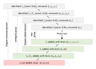
Figure 2. Recursion chain for FLITSR with Ochiai as base metric, over the test suite in Figure 1.

Iteration	$l_{2}$	$l_{3}$	$l_{4}$	$l_{5}$	l6	$l_{7}$	$l_{8}$	l9	$l_{10}$	$l_{12}$	$l_{15}$	$l_{19}$	$l_{20}$	$l_{22}$	l23	$l_{24}$	$l_{25}$	$l_{26}$	$l_{28}$
1	0.42	0.42	0.42	0.42	0.35	0.37	0.13	0.43	0.13	0.61	0.18	0.32	0.00	0.34	0.34	0.18	0.16	0.00	0.18
2	0.23	0.23	0.23	0.23	0.26	0.13	0.00	0.16	0.16	-	0.23	0.40	0.00	0.42	0.42	0.22	0.20	0.00	0.22
3	0.37	0.37	0.37	0.37	0.41	0.20	0.00	0.25	0.25	-	0.37	0.00	0.00	-	-	0.00	0.00	0.00	0.00
4	0.27	0.27	0.27	0.27	-	0.29	0.00	0.35	0.35	-	0.27	0.00	0.00	-	-	0.00	0.00	0.00	0.00
FLITSR	-	-	-	-	#2	-	-	#3	-	-	-	-	-	#1	#1	-	-	-	-

Figure 3. Ochiai scores for each FLITSR iteration in running example; the highest scores in each iteration are highlighted, and elements in the final basis boldfaced. Final ranking shown at bottom.

In the first iteration, Ochiai identifies $l_{12}$ as most suspicious; it is executed in the failing tests $c_{3}$, $c_{4}$, and $c_{5}$, which are thus removed from the test suite. In the second iteration, $l_{22}$ and $l_{23}$ both emerge as most suspicious over this reduced test suite. Note that $l_{22}$ and $l_{23}$ have identical execution spectra over the original test suite (see Figure 1) and form an ambiguity group. Hence, FLITSR adds both to the span, and removes $t_{16}$–$t_{18}$. The third iteration identifies $l_{6}$ and removes $c_{1}$. The fourth iteration identifies $l_{9}$ and $l_{10}$ as most suspicious; however, these do not form an ambiguity group over the original test suite and FLITSR applies its tie breaker rule, to pick $l_{9}$ only, since its original Ochiai score is higher than that of $l_{10}$ (see Figure 1). After $c_{2}$ is removed, the test suite contains no further failing tests, and the first phase is completed.

3.3. Phase II: Span Reduction

In the second phase, FLITSR minimizes the fault-covering set by eliminating redundant program elements, i.e., by identifying elements which can be removed from the set without compromising its fault-covering property. Elements identified in later iterations are more often required in the basis since they explain failing test cases that elements from previous iterations did not. FLITSR therefore backtracks over the iterations from the first phase and checks in sift (lines 18–26) whether the elements added to the span in the current iteration are subsumed (i.e., their failing tests are already accumulated) by elements added in later iterations (line 20) and can thus be sifted out (line 21). However, if this is not the case, FLITSR considers $e$ to be faulty, and sift sets the rank of $e$ and adds its failing tests from the original test suite to $A$, so that it accumulates all failing tests of the elements kept in the basis (line 24). This ensures that $C$ maintains the spanning property.

The basis elements are then placed at the top of the SBFL ranking, and are given an internal ranking in the order that they were selected by FLITSR. This internal ranking is based on the intuition that elements selected earlier by FLITSR are chosen based on a larger part of the test suite, and are therefore more likely to be a correct choice. The internal basis ranking also reduces the number of large ties in the ranking, which is a difficult problem in SBFL (Xu et al., 2011).

Running example. The lower half of Figure 2 illustrates the span reduction for the running example. It starts with the results of the fourth-round iteration of the first phase, i.e., the element $l_{9}$, and the failing tests $c_{2}$–$c_{5}$; note that the second phase always uses the failing tests from the original test suite, not the reduced versions. Since the accumulator $A$ is initially empty, we keep $l_{9}$ at rank #4 and add $c_{2}$–$c_{5}$ to $A$. From the third iteration we keep $l_{6}$ in the basis at rank #3, and add $c_{1}$ to $A$ (since it already contains $c_{4}$); from the second iteration, we keep $l_{22}$ and $l_{23}$ (since we cannot resolve the ambiguity group) at rank #2, and add the tests $t_{16}$–$t_{18}$ to $A$. Hence, when we return to the first iteration, $A$ already contains all failing tests that execute $l_{12}$, which means that it is reducible and can be removed. The second phase therefore ends with only the four suspicious elements $l_{6}$, $l_{9}$, $l_{22}$, and $l_{23}$.

The final call to compact (line 4) simply removes the gaps left in $R$ by elements not kept in the basis, and ensures the dense ranking shown in the final line of Figure 3. This gives an AWE for the last fault of 0.5, an improvement over all base metrics (see Figure 1).

3.4. Correctness

It is easy to see that the algorithm terminates in linear time. The SBFL metric ensures that the top-ranked element $e$ is failing at least one test (see Section 2) i.e., $F_{S,T_{i}}(e)\neq\emptyset$, unless all tests remaining in $T_{i}$ pass (i.e., $T_{i}\cap F=\emptyset$). Thus reduce removes a non-empty subset from $T_{i}$ on every call (i.e., the first part of the invariant on line 7 holds), as long as it contains at least one failing test. Since $T$ is finite, the condition on line 8 will become true in at most $T$ steps, at which point the recursion terminates, and the second phase will execute at most $T$ steps as well.

It is also easy to see that the algorithm computes a fault-covering span. reduce maintains the second part of the invariant on line 7 because it adds $e$ to $C$, so that the tests removed from $T_{i}$ are captured in $T_{i+1}$ by $F(C)$. When the condition on line 8 fails, this simplifies to the invariant at line 10. sift maintains a similar invariant (i.e., $F=A\cup F(C)$, see line 18) in a similar fashion. Note that reduce must remove all remaining failing tests $F_{S,T_{i}}(e)$ to ensure correctness; if it removes a subset $F^{\prime}\subsetneq F_{S,T_{i}}(e)$, sift is not guaranteed to compute a basis; if it removes a superset $F_{S,T_{i}}(e)\subsetneq F^{\prime}\subset F$, $C$ is not guaranteed to be a span. We can finally show that the span returned by Algorithm 1 is indeed minimal, i.e., a basis. The proof is given in the replication package.

4. Multi-Round Localization

The FLITSR core algorithm computes a single basis comprising only a few, highly suspicious elements. However, most program spectra admit multiple bases, with each giving an alternate explanation for the test failures. In this section, we describe a multi-round extension called FLITSR* which iteratively calculates additional bases, and ranks more program elements explicitly. We illustrate this extension with an extension of our running example, as shown in Figure 4 and described below.

FLITSR* is particularly useful when the program contains dominators and more than one failure-explaining basis may be required. More specifically, since a dominator, by definition (see Section 2), masks all other exposed faults that it dominates, FLITSR may fail to localize them; this occurs when the dominator is ranked by the base metric as the most suspicious element in any iteration (but the last) of the first phase, since FLITSR either removes all (remaining) failing tests executing the dominator and thus does not consider the masked faults in the first phase, or removes them from the basis in the second phase if they had already been selected.

Running example. Consider again our running example in LABEL:lst:motv1 and Figure 1. $l_{2}$ is actually faulty as well and fails with an uncaught exception if count is called with a null value. However, the original test suite does not expose this fault, and the base metrics score $l_{2}$ fairly low. If we now add to $T$ the new integration test $i_{27}$ that calls count with null (cf. Figure 4), the base metrics score $l_{2}$ higher.

#	input	l2	$l_{3}$	$l_{4}$	$l_{5}$	l6	$l_{7}$	$l_{8}$	l9	$l_{10}$	$l_{12}$	$l_{15}$	$l_{19}$	$l_{20}$	$l_{22}$	l23	$l_{24}$	$l_{25}$	$l_{26}$	$l_{28}$
$c_{1}$	"0"	✗	✗	✗	✗	✗						✗
⋮	⋮	⋮	⋮	⋮	⋮	⋮	⋮	⋮	⋮	⋮	⋮	⋮	⋮	⋮	⋮	⋮	⋮	⋮	⋮	⋮
$i_{26}$	"000"	✓	✓	✓	✓	✓						✓	✓		✓	✓	✓
t27	null	✗
Tarantula		0.48	0.44	0.44	0.44	0.67	0.42	0.25	0.53	0.22	1.00	0.24	0.43	0.00	0.46	0.46	0.40	0.33	0.00	0.40
Ochiai		0.46	0.39	0.39	0.39	0.33	0.34	0.13	0.40	0.12	0.58	0.17	0.30	0.00	0.32	0.32	0.17	0.15	0.00	0.17
DStar		2.25	1.47	1.47	1.47	0.44	1.00	0.07	1.33	0.07	1.50	0.20	0.64	0.00	0.69	0.69	0.09	0.08	0.00	0.09
1.1		0.46	0.39	0.39	0.39	0.33	0.34	0.13	0.40	0.12	0.58	0.17	0.30	0.00	0.32	0.32	0.17	0.15	0.00	0.17
1.2		0.31	0.21	0.21	0.21	0.24	0.12	0.00	0.14	0.14	-	0.21	0.37	0.00	0.39	0.39	0.20	0.18	0.00	0.20
1.3		0.43	0.30	0.30	0.30	0.33	0.17	0.00	0.20	0.20	-	0.30	0.00	0.00	-	-	0.00	0.00	0.00	0.00
FLITSR		#2	-	-	-	-	-	-	-	-	-	-	-	-	#1	#1	-	-	-	-
2.1		-	0.42	0.42	0.42	0.35	0.37	0.13	0.43	0.13	0.61	0.18	0.32	0.00	-	-	0.18	0.16	0.00	0.18
2.2		-	0.23	0.23	0.23	0.26	0.13	0.00	0.16	0.16	-	0.23	0.40	0.00	-	-	0.22	0.20	0.00	0.22
2.3		-	0.37	0.37	0.37	0.41	0.20	0.00	0.25	0.25	-	0.37	-	0.00	-	-	0.00	0.00	0.00	0.00
2.4		-	0.27	0.27	0.27	-	0.29	0.00	0.35	0.35	-	0.27	-	0.00	-	-	0.00	0.00	0.00	0.00
3.1		-	0.45	0.45	0.45	-	0.39	0.14	-	0.13	0.65	0.20	-	0.00	-	-	0.19	0.17	0.00	0.19
3.2		-	0.26	0.26	0.26	-	0.14	0.00	-	0.18	-	0.26	-	0.00	-	-	0.25	0.22	0.00	0.25
3.3		-	-	-	-	-	0.00	0.00	-	0.00	-	0.00	-	0.00	-	-	0.35	0.32	0.00	0.35
3.4		-	-	-	-	-	0.00	0.00	-	0.00	-	0.00	-	0.00	-	-	-	0.45	0.00	0.50
4.1		-	-	-	-	-	0.42	0.15	-	0.14	0.71	0.21	-	0.00	-	-	-	0.18	0.00	-
4.2		-	-	-	-	-	0.17	0.00	-	0.20	-	0.30	-	0.00	-	-	-	0.26	0.00	-
4.3		-	-	-	-	-	0.00	0.00	-	0.00	-	-	-	0.00	-	-	-	0.45	0.00	-
5.1		-	-	-	-	-	0.52	0.19	-	0.18	-	-	-	0.00	-	-	-	-	0.00	-
6.1		-	-	-	-	-	-	0.27	-	0.25	-	-	-	0.00	-	-	-	-	0.00	-
6.2		-	-	-	-	-	-	-	-	0.35	-	-	-	0.00	-	-	-	-	0.00	-
FLITSR∗		#2	#6	#6	#6	#4	#12	#13	#5	#14	#9	#10	#3	-	#1	#1	#7	#11	-	#8

Figure 4. Spectrum (top block) and suspiciousness scores for running example with extended test suite. Scores for base metrics shown in second block, Ochiai scores for FLITSR and FLITSR* rounds in third and fourth blocks. Highest scores in each iteration are highlighted, and elements in any computed basis are boldfaced. Final ranking shown at bottom.

However, if we run FLITSR using this extended test suite $T^{\prime}$, we encounter $l_{2}$ early on, and since it is a dominator for count, FLITSR constructs an “impoverished” basis, which leaves too many (faulty) elements unranked. Consider for example FLITSR’s run using Ochiai, as detailed in the lower part of Figure 4. As before (i.e., without $i_{27}$), FLITSR first selects $l_{12}$, then $l_{22}$ and $l_{23}$ in the first two iterations of its first phase, removing the corresponding test failures $\{c_{3},c_{4},c_{5},t_{16},t_{17},t_{18}\}$ from $T^{\prime}$. In the third iteration, it identifies $l_{2}$ as most suspicious, due to the failing test case $i_{27}$; however, since this is a dominator for count, FLITSR removes all remaining test failures $c_{1}$, $c_{2}$, and $i_{27}$ and terminates its first phase. In the second phase, it identifies $l_{12}$ as redundant. The basis returned by FLITSR is thus just $\{l_{2},l_{22},l_{23}\}$, with $l_{2}$ at rank #2, as given in Figure 4. Hence, FLITSR fails to localize the faults $l_{6}$ and $l_{9}$ due to the presence of the exposed dominator and its performance degrades.

FLITSR*. We can prevent this performance degradation by running multiple FLITSR rounds over increasingly smaller subsets of the SUT’s elements and test suite. Each round then returns a less suspicious basis for the remaining test failures. The elements in each round’s basis $C_{i}$ are ranked just below those of the previous round.

We remove the basis $C_{i}$ before the next round, i.e., do not compute any scores for these elements. We also remove the failing tests that are executed only by elements in $C_{i}$ to prevent these now “unexplainable” test failures from influencing the scores computed in the next round. We repeat this process until a round can no longer compute a basis, i.e., until all elements executing a failing test have been added to a basis and thus been ranked explicitly.

Algorithm 2 FLITSR^∗ multi-round algorithm

1:$M$ $\triangleright$ base scoring method

2:$S_{0}$ $\triangleright$ system under test

3:$T_{0}$ $\triangleright$ initial test suite

4:$C^{*}$ $\triangleright$ basis list

5:$C^{*}$ $\leftarrow$ $\langle\rangle$

6:flitsr^∗($S_{0},T_{0}$)

7:function flitsr*($S_{i}$, $T_{i}$)

8:    $C$, _ $\leftarrow$ flitsr($M,S_{i},T_{i}$) $\triangleright$ Algorithm 1

9:    if $C\neq\emptyset$ then

10:          $C^{*}$ $\leftarrow$ $C^{*}+\!\!\!+\,\langle C\rangle$ $\triangleright$ append basis with lowest rank

11:          $S^{\prime}_{i}$ $\leftarrow$ $S_{i}\setminus C$ $\triangleright$ remove from coverage matrix

12:          $R$ $\leftarrow$ $F_{S_{i},T_{i}}(C)\setminus F_{S_{i},T_{i}}(S^{\prime}_{i})$ $\triangleright$ tests failing in basis only

13:          $T^{\prime}_{i}$ $\leftarrow$ $T_{i}\setminus R$ $\triangleright$ remove from coverage matrix

14:         flitsr^∗($S^{\prime}_{i},T^{\prime}_{i}$)

15:    end if

16:end function

Algorithm 2 shows the algorithm’s details. It reuses Algorithm 1 with minor changes as basic building block. In particular, we now require the algorithm to maintain and use an offset in the rank assignments, to ensure that later bases are ranked lower.

Running example. The lower part of Figure 4 shows the detailed Ochiai scores in the subsequent rounds of FLITSR^∗ for our running example. Entries dashed across the entire block denote the elements removed in a previous round.

In the first round, FLITSR identifies the basis $C_{1}=\{l_{2},l_{22},l_{23}\}$. These elements (in fact, $l_{2}$) exclusively execute the failing test $t_{27}$, so for the second round we remove $C_{1}$ from $S$ and $F_{S,T}(C_{1})\setminus F_{S,T}(S\backslash C_{1})=\{t_{27}\}$ from $T$, for the new SUT $S_{1}$ and test suite $T_{1}$, respectively. This second round identifies the basis $C_{2}=\{l_{6},l_{9},l_{19}\}$. All failing tests remaining in $T_{1}$ that are executed by elements in $C_{2}$ are also executed by elements remaining in $S_{1}$ that are not in $C_{2}$, so we start the third round with $S_{1}\setminus C_{2}$ and $T_{1}$. The following rounds identify the elements shown in bold in the table as basis and remove them and the associated failing test. After the sixth round no failing tests remain, and FLITSR returns an empty basis, so we terminate the (outer) FLITSR^∗ loop.

Using the ranking in the last line of Figure 4 gives us an AWE_L of 2, which is a substantial improvement over both FLITSR’s single-round result of 12.33, and the Ochiai result of 5.

5. Experimental Evaluation

5.1. Research Questions

With our experimental evaluation, we aim to answer the following research questions:

RQ1:

How much does FLITSR improve on existing SBFL methods?

RQ2:

How much are the results dependent on the applied base metric? Which base metric, if any, induces the best results?

RQ3:

How much does FLITSR improve on learning-based methods?

RQ4:

What effect does the multi-round variant FLITSR^∗ have on the improvements?

RQ5:

What effect do the fault type (real or injected) and coverage granularity have on the results of FLITSR and FLITSR*?

5.2. Experimental Setup

5.2.1. Synthetic Fault Data Set

Our first experimental dataset is based on variants of 15 Java-based open-source systems analyzed by Steimann and Frenkel (Hogerle et al., 2014; tcm, [n. d.]). Each variant differs from its respective baseline system by a number of synthetic faults injected into its methods by repeatedly applying simple mutation operators. The number $N_{f}$ of injected faults follows a geometric progression; the number of resulting variants is $m_{1}\leq 600$ resp. $m_{n}=5000,n=2,4,8,16,32$, for a total of 75000 $n$-fault variants.

Each variant was executed over its respective baseline test suite, which range in size from 55 (JDepend) to 1666 (Daikon) tests ($\mu\!\>=\!\>345,\sigma^{2}\!\>=\!\>403$). However, not all methods are exercised by the test suites, and the spectra contain between 152 (Jester) and 2075 (Lang) methods ($\mu\!\>=\!\>698,\sigma^{2}\!\>=\!\>589$).

5.2.2. Real Fault Data Set

Table 1. Defects4J (1.5.0) multi-fault benchmark characteristics; cf. (An et al., 2021) for included bug ids. $N$ is the number of versions in each project.

		Size (methods / stmts.)				Tests (pass / fail)				Faults
Project	$N$	min	max	min	max	min	max	min	max	min	avg	max
Chart	26	3466	4135	62113	79788	1578	6486	1	24	1	3.39	5
Closure	104	3294	5520	27412	45109	2591	7821	7	81	2	9.10	14
Lang	64	1538	2022	8909	11190	1593	2658	2	35	2	6.10	12
Math	106	745	4029	4809	38688	876	5184	2	34	1	4.90	10
Time	26	1732	1797	9898	10917	3745	3996	6	54	2	6.94	10

Our second experimental dataset is based on Defects4J (v1.5.0) (Just et al., 2014a), a collection of real-world faults extracted from five medium-sized (20–100 kLoC) Java-based open-source systems. Each fault is given in the form of a diff file that repairs the faulty base version, and is accompanied by a test suite that exposes this fault only. The variants in Defects4J are not necessarily single-fault systems, since faults from later versions can already be present in earlier ones. However these multiple faults are not identified in each version since the test cases that expose the faults do not initially exist in that version. An et al. (An et al., 2021) use an iterative search approach to “transplant” the fault-exposing tests across versions in order to identify versions within the Defects4J dataset that already contain multiple faults. From this, they detect 311 existing multi-fault versions within the Defects4J dataset.

However, the test transplantation by An et al.(An et al., 2021) does not provide the localization oracle that is required to evaluate the performance of a fault localizer: it only guarantees that tests that expose a fault $f_{i}$ in a more recent system variant $v_{i}$ also fail in the older variant $v_{j}$, but does not specify where in $v_{j}$ the fault $f_{i}$ is located.

We therefore apply a fault location translation process that augments the test transplantation. For this process, we identify all lines in the diff that repairs $f_{i}$ in $v_{i}$ as faulty lines pertaining to that bug. We then locate these lines in the earlier version $v_{j}$ (where the lines may have been moved), by considering the diffs in the full project history in order, updating the line numbers if their position has changed. If a line is either not executable, or modified during the history of the project between the versions, we consider the line no longer necessarily identifying for the fault, and therefore remove it from consideration. If all the lines in a fault-fixing diff have been dropped in this way, a characteristic location for the fault cannot be given, and we therefore remove this fault from the experimental evaluation. In this way, we get a subset of all faults identified by An et al. (An et al., 2021) in each version. Note that we do not alter any Defects4J version, but merely identify the statements in a version that pertain to a bug that has been described in a later version. This is in contrast to Zheng et al. (Zheng et al., 2018), who created synthetic multi-fault versions by transplanting faults. Table 1 summarizes our dataset; it is available at https://github.com/DCallaz/defects4j_multifault.

5.2.3. Data Collection

For the first dataset, we used the method-level execution spectra provided by Steimann and Frenkel (Hogerle et al., 2014; tcm, [n. d.]), in the form of TCMs. For the second dataset, we compiled the (faulty) sources using the Defect4J compile script and relied on GZoltar (v1.7.3) (Campos et al., 2012) to collect coverage information for each of the variants. We condensed this into method- and statement-level spectra.

For each spectrum we computed eight single fault metrics (Tarantula, Ochiai, DStar, Jaccard, GP13, naish2, Overlap, and Harmonic) and three multi-fault metrics (Zoltar, Hyperbolic and Barinel), and ran both FLITSR and FLITSR* using each of these as base metric. For each metric (including all FLITSR variants) we produced a single suspiciousness ranking per spectrum. We evaluated the metrics based on the rankings without attempting to fix any faults.

We also compare to the state-of-the-art learning-based tool GRACE, which has been shown to outperform other learning-based techniques (Lou et al., 2021). For this comparison, we ran the existing implementation of GRACE (which identifies method-level faults only) as a black-box over the five Defects4J projects we use in our evaluation. Note that the actual Defects4J code bases are identical to those used for the original evaluation of GRACE (Lou et al., 2021), with the only difference being the test suite supplied for each version. Note also that FLITSR runs almost instantaneously, once the coverage data is collected, while GRACE spent several hours on optimizing its predictions, and failed to terminate within 24 hours for Closure.

5.3. Method-Level Localization Results

Table 2. Method-level results for 15 Java projects (Hogerle et al., 2014) averaged over all variants with given number $N_{f}$ of mutations. Metrics designed for multi-fault localization are shown in the last three rows. Improvements of FLITSR and FLITSR* variants over corresponding base metrics are highlighted in yellow. Best results in each column are shown in bold.

	$N_{f}=1$			$N_{f}=2$				$N_{f}=4$				$N_{f}=8$				$N_{f}=16$				$N_{f}=32$
Metric	AWE1	P@5	R @ $N_{\!f\!}$	AWE1	AWE2	P@5	R @ $N_{\!f\!}$	AWE1	AWEM	P@5	R @ $N_{\!f\!}$	AWE1	AWEM	P@5	R @ $N_{\!f\!}$	AWE1	AWEM	P@5	R @ $N_{\!f\!}$	AWE1	AWEM	P@5	R @ $N_{\!f\!}$
FLITSR (T)	25.4	8.3	39.9	16.3	65.5	14.1	33.1	10.4	42.6	22.6	29.7	7.0	48.3	28.6	28.0	4.9	52.6	31.0	28.4	3.1	52.6	33.0	31.2
FLITSR (O)	19.7	10.3	41.9	12.0	60.3	18.1	35.6	8.5	40.1	26.4	31.7	6.3	49.1	30.5	29.5	5.0	61.2	31.6	28.5	3.4	65.1	32.6	29.7
FLITSR (H)	17.2	10.4	42.1	12.2	61.9	17.9	35.6	8.6	38.9	26.2	31.8	6.1	45.5	30.7	29.7	4.5	52.9	32.5	29.2	3.1	55.0	33.5	31.1
FLITSR* (T)	21.7	10.2	39.9	13.3	54.5	17.8	33.2	9.0	33.6	25.1	29.8	6.3	37.9	28.8	28.1	4.4	42.8	31.0	28.6	3.0	44.2	33.0	31.5
FLITSR* (O)	19.9	10.8	41.9	12.0	52.0	18.9	35.6	8.0	32.0	26.8	31.8	5.8	37.4	30.6	29.7	4.7	45.4	31.7	29.1	3.2	48.5	32.6	30.8
FLITSR* (H)	17.3	10.8	42.1	12.1	49.2	18.9	35.6	8.3	31.9	26.8	31.8	5.8	37.1	30.8	29.8	4.3	43.2	32.6	29.5	3.1	45.5	33.5	31.5
Tarantula (Jones et al., 2002)	29.7	7.3	22.2	23.9	71.6	10.1	14.3	20.5	54.2	11.1	11.5	16.7	64.9	11.4	11.3	12.2	72.3	13.2	13.1	7.9	75.9	17.4	17.3
Ochiai (Abreu et al., 2006)	19.7	10.3	40.5	12.4	74.0	14.7	29.9	10.1	64.7	16.6	21.5	8.8	89.5	16.5	15.7	8.3	102.8	16.3	13.2	6.7	104.1	17.7	15.1
DStar (Wong et al., 2014)	19.5	10.6	41.3	12.5	83.0	14.6	29.9	11.1	77.5	15.3	20.1	10.5	105.9	14.2	13.5	10.2	114.7	14.0	11.5	7.8	112.0	16.0	14.1
Jaccard (Chen et al., 2002)	20.7	10.2	40.1	12.9	77.7	14.6	29.7	10.4	70.5	16.1	21.0	9.2	100.6	15.5	14.7	8.9	113.6	15.2	12.2	7.3	111.8	16.6	14.2
GP13 (Yoo, 2012)	18.5	11.2	43.5	22.4	95.3	11.2	22.2	22.8	88.1	10.3	13.0	18.2	108.6	10.2	10.4	13.5	115.0	11.5	10.4	8.8	112.0	14.8	13.9
Naish2 (Naish et al., 2011)	15.8	11.2	43.5	22.2	92.0	11.2	22.2	22.8	87.8	10.3	13.0	18.2	108.6	10.2	10.4	13.5	115.0	11.5	10.4	8.8	112.0	14.8	13.9
Overlap (Heiden et al., 2019)	39.8	4.5	11.6	29.5	83.9	7.8	11.4	22.0	60.6	10.4	10.8	16.8	67.8	11.2	11.2	12.2	72.9	13.2	13.0	7.9	75.9	17.4	17.3
Harmonic (Lee, 2011)	17.2	10.4	40.7	12.5	70.0	14.5	29.5	9.9	52.6	17.0	22.1	7.6	66.3	18.3	17.5	6.6	76.2	19.2	15.9	5.4	81.5	20.9	17.9
Zoltar-s (Abreu et al., 2009a)	18.8	10.5	41.5	16.8	71.1	12.7	24.7	12.7	52.4	14.9	19.1	8.8	64.2	16.8	16.4	6.3	72.4	19.5	16.4	4.6	77.3	22.2	18.9
Hyperbolic (Neelofar et al., 2018)	18.4	11.1	43.4	20.1	82.5	12.0	24.0	17.7	66.2	13.1	16.7	13.3	75.0	14.1	14.0	10.2	79.5	15.7	13.9	6.8	82.0	18.8	17.2
Barinel (Abreu et al., 2009b)	629.1	0.0	0.0	310.5	518.5	0.4	0.4	168.9	363.2	0.9	0.9	84.1	318.0	2.2	2.2	40.6	266.9	4.9	4.9	19.4	221.1	9.9	9.9

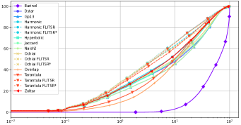
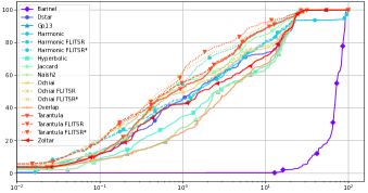
Figure 5. Percentage of bugs found over proportion of methods inspected in rank order, x-axis shown in log-scale. (Top) averaged over synthetic fault dataset (Hogerle et al., 2014). (Bot) averaged over Defects4J multi-fault dataset.

The graphs in Figure 5 plot the percentage of faults found with respect to the percentage of methods inspected, over all projects in each of the datasets and for all base metrics and a subset of FLITSR and FLITSR* variants. We use a log-scale for the x-axis to highlight the differences at the higher parts of the ranking since developers only inspect a small number of the program elements in order (Parnin and Orso, 2011). We only plot a sample of the FLITSR and FLITSR* variants because there is little variance in the remaining results. Specifically, we show results for Tarantula and Ochiai, due to their popularity in the literature, and Harmonic mean, since its FLITSR and FLITSR* variants performed well.

Figure 5 shows that the FLITSR variants find a larger fraction of the faults at a smaller fraction of the methods inspected than the corresponding base metrics, and that FLITSR* amplifies this trend and outperforms FLITSR after the inspection of 0.5–1% of the methods. We also note that even for base metrics that perform quite differently (cf. Figure 5 for Ochiai versus Tarantula), their FLITSR and FLITSR* variants perform surprisingly similar. A comparison of the two graphs shows that all techniques perform substantially better for real faults than for synthetic faults; for example, at 1% of the methods inspected FLITSR* already identifies about 62% of the real faults, compared to about 28% of the synthetic faults.

Tables 2 and 3 show more detailed results. We include the AWEs at different levels, as appropriate, as well as precision and recall (cf. Section 2 for definitions). For the TCM dataset, we aggregated the data over the different fault injection bins. Here, we use $R@N_{f}$, where $N_{f}$ is the number of injected faults, and $P@5$. For the Defects4J dataset, we aggregated the data over the individual projects. Here, we always use $R@10$ (because the average number $\overline{N}{\!{}_{f}}$ of faults per variant is less than ten), $P@5$ and $P@1$; the latter shows how often the fault localizer pinpoints at least one fault.

Table 3. Method-level results for Defects4J multi-fault dataset averaged over all variants per project. See Table 2 for notation.

	Chart ($\overline{|S|}=3649$, $\overline{N}{\!{}_{f}}=3$)					Closure ($\overline{|S|}=5155$, $\overline{N}{\!{}_{f}}=9$)					Lang ($\overline{|S|}=1745$, $\overline{N}{\!{}_{f}}=6$)					Math ($\overline{|S|}=2733$, $\overline{N}{\!{}_{f}}=5$)					Time ($\overline{|S|}=1769$, $\overline{N}{\!{}_{f}}=7$)
Metric	AWE1	AWEM	R@10	P@1	P@5	AWE1	AWEM	R@10	P@1	P@5	AWE1	AWEM	R@10	P@1	P@5	AWE1	AWEM	R@10	P@1	P@5	AWE1	AWEM	R@10	P@1	P@5
FLITSR (T)	0.3	4.1	78.3	67.5	44.8	93.2	574.8	2.3	3.6	3.2	4.3	28.3	34.8	44.2	18.5	1.0	12.2	64.8	57.1	29.7	5.2	47.5	16.3	0.0	16.2
FLITSR (O)	2.1	22.7	65.1	32.5	31.9	97.2	924.9	2.5	0.0	3.3	3.0	30.5	34.9	59.8	21.2	1.0	13.2	63.7	76.6	34.5	5.1	187.1	13.4	43.4	12.7
FLITSR (H)	1.7	20.8	62.8	41.2	37.5	105.7	714.2	2.4	1.1	3.1	3.8	30.4	31.4	45.9	16.7	1.9	24.3	58.9	45.6	26.6	3.0	190.7	17.1	43.4	13.6
FLITSR* (T)	0.3	5.2	74.7	67.5	45.3	50.9	520.1	2.8	3.6	3.3	3.8	21.8	36.6	44.2	19.3	1.0	12.0	65.0	57.1	29.6	5.2	25.0	16.3	0.0	16.5
FLITSR* (O)	2.1	7.1	61.5	32.5	32.2	48.4	643.3	3.0	0.0	3.4	3.0	24.5	36.1	59.8	22.0	1.0	12.5	65.2	76.6	34.4	5.1	19.3	16.3	43.4	12.7
FLITSR* (H)	1.7	7.0	60.3	41.2	37.8	50.0	652.5	4.7	1.1	3.3	3.8	24.7	32.9	45.9	17.1	1.9	19.2	57.3	45.6	27.2	3.0	27.3	23.2	43.4	13.6
Tarantula	3.2	11.9	60.0	31.6	31.8	96.0	573.6	2.5	1.5	2.5	4.8	28.2	36.1	27.5	20.3	2.4	17.2	49.6	29.9	24.6	5.2	69.3	15.6	0.0	15.4
Ochiai	5.4	37.5	48.9	24.6	22.5	108.1	922.6	1.3	0.5	1.8	3.7	30.5	31.5	45.4	18.8	2.5	19.8	46.8	55.8	28.7	2.5	254.7	19.7	43.4	19.8
DStar	5.7	86.2	38.5	22.9	20.6	140.7	987.5	0.6	0.0	0.5	10.3	29.4	28.9	48.1	17.3	5.3	32.1	41.9	55.8	21.4	12.7	402.1	23.7	43.4	17.3
Jaccard	5.5	57.6	40.2	24.1	21.8	98.9	586.3	0.8	0.0	1.4	7.9	31.5	27.5	58.8	17.1	3.6	18.2	47.9	49.7	23.5	3.2	112.5	26.3	43.4	17.1
GP13	12.3	139.7	34.8	7.5	16.5	445.4	1165.7	0.0	0.0	0.0	12.6	30.7	28.2	46.5	15.6	24.7	49.4	17.8	49.7	8.0	413.4	659.5	0.0	0.0	0.0
Naish2	12.3	139.7	34.8	7.5	16.5	445.4	1155.5	0.0	0.0	0.0	12.6	30.7	28.2	46.5	15.6	24.7	46.7	17.8	49.7	8.0	413.4	659.5	0.0	0.0	0.0
Overlap	6.4	48.3	41.7	29.1	26.5	430.9	1217.4	0.1	0.2	0.2	6.3	40.6	26.0	24.0	17.0	10.1	53.1	29.0	29.2	20.0	262.3	576.7	0.0	0.0	0.0
Harmonic	5.7	30.4	55.3	34.4	30.7	116.1	713.1	1.4	0.0	2.0	3.8	29.1	31.8	35.3	19.2	3.0	25.5	45.7	29.2	25.2	4.9	224.7	18.3	34.7	14.5
Zoltar-s	3.4	27.7	55.6	35.7	32.2	264.6	1023.6	1.2	1.7	1.0	3.6	29.4	31.7	35.3	19.3	2.6	20.4	46.2	29.5	25.3	79.9	439.4	4.2	0.0	5.2
Hyperbolic	8.1	42.4	45.6	24.1	19.5	446.5	1147.9	0.0	0.0	0.0	4.2	29.1	32.1	33.6	18.4	8.2	40.2	27.9	23.4	17.9	322.9	633.3	0.0	0.0	0.0
Barinel	1717.4	3288.4	0.1	0.0	0.0	3772.9	4813.6	0.0	0.0	0.0	1217.9	1915.2	0.1	0.0	0.0	1863.5	3323.6	0.1	0.0	0.0	1407.3	2557.0	0.0	0.0	0.0
GRACE	35.5	98.8	9.7	10.0	5.0	(aborted after 24 hours)					7.2	48.2	22.7	26.2	18.6	22.2	87.9	12.5	10.5	5.0	296.1	701.8	0.4	5.2	1.0

Table 4. Statement-level results for Defects4J multi-fault dataset averaged over all variants per project. See Table 2 for notation.

	Chart ($\overline{|S|}=67570$, $\overline{N}{\!{}_{f}}=3$)					Closure ($\overline{|S|}=41969$, $\overline{N}{\!{}_{f}}=9$)					Lang ($\overline{|S|}=9719$, $\overline{N}{\!{}_{f}}=6$)					Math ($\overline{|S|}=23740$, $\overline{N}{\!{}_{f}}=5$)					Time ($\overline{|S|}=10289$, $\overline{N}{\!{}_{f}}=7$)
Metric	AWE1	AWEM	R@10	P@1	P@5	AWE1	AWEM	R@10	P@1	P@5	AWE1	AWEM	R@10	P@1	P@5	AWE1	AWEM	R@10	P@1	P@5	AWE1	AWEM	R@10	P@1	P@5
FLITSR (T)	7.4	60.1	24.6	24.0	13.4	36.9	1806.6	15.5	38.8	21.7	35.5	151.5	5.6	2.4	1.7	3.9	130.5	34.3	36.1	16.6	3.2	186.8	18.5	56.5	14.3
FLITSR (O)	7.1	119.4	25.3	26.2	13.3	58.4	2920.3	14.6	3.9	15.5	28.8	175.4	7.6	4.8	3.5	7.0	141.0	24.8	27.2	11.4	5.7	676.4	18.8	21.7	15.6
FLITSR (H)	7.1	106.7	25.7	26.2	14.4	126.2	2561.1	12.9	17.8	17.6	32.0	168.7	7.5	4.1	3.6	4.2	86.2	31.2	33.2	15.2	6.1	582.0	18.6	43.4	14.6
FLITSR* (T)	7.4	36.1	24.6	24.0	14.2	22.2	1461.6	15.5	38.8	21.7	31.0	125.6	5.6	2.4	1.7	3.9	129.2	34.3	36.1	16.6	3.2	94.4	18.5	56.5	14.3
FLITSR* (O)	7.1	39.9	25.3	26.2	13.3	21.4	1717.9	14.6	3.9	15.5	26.0	110.7	7.5	4.8	3.5	8.3	142.3	23.8	27.2	11.4	5.7	74.4	18.8	21.7	15.6
FLITSR* (H)	7.1	39.3	25.6	26.2	14.3	51.0	2241.2	13.0	17.8	17.6	30.2	137.2	7.5	4.1	3.6	4.2	84.4	31.3	33.2	15.2	5.0	136.0	20.6	43.4	14.6
Tarantula	20.3	64.6	16.2	6.3	6.6	60.0	1803.9	13.2	13.7	12.5	38.8	149.7	4.9	1.4	1.9	7.2	145.1	26.1	14.2	12.9	5.7	185.9	14.5	8.5	10.2
Ochiai	14.6	192.9	17.7	26.9	6.0	147.8	2916.2	2.4	13.7	2.4	33.8	174.4	6.7	4.8	2.2	10.1	162.9	19.4	17.6	7.8	12.3	697.6	17.2	21.7	11.1
DStar	15.4	433.7	16.1	26.4	4.6	528.5	3792.5	0.5	1.7	0.2	76.1	193.6	8.1	6.0	2.1	59.5	305.6	10.0	17.6	2.6	82.6	1486.3	18.1	21.7	10.1
Jaccard	15.0	294.1	17.4	26.9	5.1	204.5	1865.2	0.6	1.7	0.6	61.1	183.2	9.7	6.0	2.4	13.6	163.8	15.3	2.1	4.3	17.2	412.3	17.6	21.7	10.1
GP13	53.8	731.0	14.4	15.0	2.9	2172.0	5869.1	0.3	0.5	0.1	84.8	209.5	7.3	5.9	3.8	251.6	449.6	2.9	1.2	0.8	1477.4	2517.0	0.0	0.0	0.0
Naish2	53.8	731.0	14.4	15.0	2.9	2172.0	5811.7	0.3	0.5	0.1	84.8	209.5	7.3	5.9	3.8	251.6	391.7	2.9	1.2	0.8	1477.4	2517.0	0.0	0.0	0.0
Overlap	36.9	228.7	14.1	6.1	6.1	628.7	5110.3	6.8	8.9	6.9	50.3	258.7	2.9	1.5	1.5	30.6	356.5	19.9	13.7	11.4	240.2	2043.8	4.4	6.5	6.5
Harmonic	15.2	135.1	22.1	26.6	13.6	126.9	2559.9	10.1	17.4	9.7	33.6	167.2	3.5	2.6	1.7	8.3	114.5	24.3	21.7	12.7	6.3	581.7	15.8	21.7	9.0
Zoltar-s	10.5	146.8	23.2	24.5	14.4	336.6	3361.4	13.0	20.3	12.3	32.7	171.2	3.6	2.6	1.7	7.2	161.9	24.4	21.8	12.4	129.1	1439.1	6.6	4.3	4.3
Hyperbolic	27.8	202.4	16.5	26.1	7.1	1670.8	4480.0	0.3	0.5	0.1	36.1	180.5	3.0	2.6	1.7	54.6	294.7	13.1	19.4	9.5	1052.8	2207.5	0.0	0.0	0.0
Barinel	9979.5	19104.6	0.0	0.0	0.0	5859.1	25366.1	0.0	0.0	0.0	4698.2	8210.1	0.0	0.0	0.0	8109.5	18124.6	0.0	0.0	0.0	1936.0	7493.5	0.0	0.0	0.0

Synthetic Faults. The results in Table 2 show that all FLITSR and FLITSR* variants perform very well for multi-fault versions ($N_{f}\geq 2$). AWE₁ ranges from 12-16 methods for $N_{f}=2$, depending on the applied base metric, to approximately 3 methods (i.e., 0.5% of the average project size) for $N_{f}=32$, confirming that it is easier to find a fault if there are more to choose from (DiGiuseppe and Jones, 2011). $P@5$ grows similarly, from appproximately 18% to approximately 33%, while $R@N_{f}$ remains mostly stable around 30%. However, the AWE_M values increase with growing fault numbers, from approximately 30–40 for $N_{f}=4$ to approximately 45–65 for $N_{f}=32$, showing that the multi-fault localization problem is hard indeed.

The highlighted entries show that for the multi-fault versions ($N_{f}\geq 2$) all FLITSR and FLITSR* variants substantially outperform all base metrics in all measures, including Zoltar-s, Hyperbolic, and Barinel, which were designed to handle multi-fault programs. Moreover, the performance difference generally grows with growing fault numbers. For example, for FLITSR* using Harmonic as base metric, the AWE₁ improvement grows from 3.2% (for $N_{f}=2$) to 42.5% (for $N_{f}=32$), AWE_M from 29.7% to 46.7%, P@5 from 30.3% to 60.2%, and R@$N_{f}$ from 30.3% to 60.2%. However, in some cases the growth levels out at smaller fault levels. At $N_{f}=1$, FLITSR no longer outperforms all base metrics for all measures, but any regressions remain small. This is expected because our approach targets multi-fault systems.

Defects4J. Table 3 shows that the results for the Defects4J dataset vary considerably between the individual projects. For Chart and Math, most base metrics already perform well, but FLITSR still yields substantial AWE reductions to the first (30%-90%) and median (30%-75%) faults, and similar increases in recall (generally around 30%) and precision (generally 20%-50%). AWE₁ is below 2.0, with $P@1$ reaching up to almost 80%, which means that FLITSR pinpoints the top error in four out of five variants. FLITSR* yields further improvements for AWE_M of up to 70% compared to the base FLITSR, and 80% compared to the corresponding base metric. For the remaining three projects, FLITSR* shows drastic improvement over FLITSR, i.e., these projects have dominating faults that require repeated localization rounds. For Lang and Closure FLITSR* yields improvements to the first fault (e.g., a 50% AWE₁ reduction for Closure), and reasonable improvements to the median fault (10%-30%); for Time it yields better improvements to the median fault (60%-90%), and no improvement for the first fault.

The bottom row of Table 3 shows the results for GRACE. It performs much worse on our multi-fault Defects4J dataset variant than the published results on the original Defects4J (Lou et al., 2021) would indicate. It is outperformed by all FLITSR-variants on almost all measures; in particular, FLITSR and FLITSR* have much smaller AWEs to the first and median faults. This may indicate that GRACE may not generalize well to multiple fauts.

5.4. Statement-Level Localization Results

Figure 6 shows the statement-level results for the Defects4J dataset. Overall, it confirms the method-level results (cf. Figure 5): FLITSR* outperforms FLITSR for each base metric, which in turn outperforms the base metric itself. Since there are generally 10$\times$ more statements than methods, the AWEs are still higher and precision and recall values are lower (cf. Table 4).

The individual project results in Table 4 show that the FLITSR* variants indeed consistently outperform the base metrics.

5.5. Statistical Analysis

We performed a non-parametric paired significance test (Wilcoxon signed-rank test) on the AWE numbers. For the synthetic faults, this shows that both FLITSR-variants statistically significantly (p¡¡0.05) outperform the respective base metrics in aggregate over all fault densities (and FLITSR* outperforms FLITSR); however, for single-fault programs and lower fault densities ($N_{\!f}=2$) the differences for some individual metrics are not statistically significant. For real faults, both FLITSR-variants again statistically significantly outperform the respective base metrics to the first fault (when aggregated over all projects), and while FLITSR* statistically significantly outperforms the base metrics to the median fault, FLITSR does not.

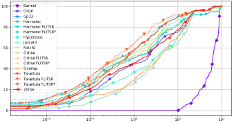
Figure 6. Percentage of bugs found over proportion of statements inspected in rank order, averaged over Defects4J multi-fault dataset. x-axis shown in log-scale.

5.6. Threats to Validity

Internal Validity. There are several threats to the internal validity of our evaluation. We carefully tested and documented our implementation, data collection and evaluation scripts to mitigate against implementation errors. We also make a replication package (rep, 2023) available. We ran GRACE as a black-box system using its default settings, which may not be optimal, but due to the complexity of its implementation we cannot tell.

The main threat is ground truth errors in the execution spectra and the actual fault locations. For the method-level dataset, we cannot judge whether the TCMs faithfully reflect actual system executions, and we have to accept them as ground truth. For the Defects4J dataset, we relied on GZoltar (Campos et al., 2012) to collect execution spectra, which is widely used in the literature (e.g., (Pearson et al., 2017; Xuan and Monperrus, 2014; Liu et al., 2019)), but is prone to potential imprecisions in the collection of statement-level execution data, which may affect the results. We discard non-executed statements labelled as fault locations, and discard faults that only affect non-executed statements to minimize bias effects. Similarly, our fault location oracle is based on the statements that are identified by the translation process (cf. Section 5.2.2);

Finally, residual faults not exposed by the test suites can still impact execution through fault masking. However, any such residual faults affect all applied approaches (if not necessarily to the same extent), which mitigates their impact.

External Validity. Our results may not necessarily generalize beyond our experimental set-up. The main threats stem from the execution spectra, the fault types, and the applied metrics. Our evaluation uses simple program execution spectra derived from Java-based systems. Spectra derived from other languages (Wong et al., 2014; Abreu et al., 2009c; Wang et al., 2020; Khan et al., 2021; Troya et al., 2018; Raselimo and Fischer, 2019) or involving more complex types of elements (e.g., data flow edges (Santelices et al., 2009)) could have different characteristics that impact the results.

Our method-level evaluation partly relies on mutation-based fault injection (Steimann et al., 2013). There is some evidence (Just et al., 2014b; Papadakis et al., 2018) that they may be a valid substitute for real faults in software testing, but Figure 5 shows that the localization results differ substantially, although the general trends remain similar. Tables 3 and 4 show that different real-world projects lead to quite different results; other projects with different fault characteristics may not support our conclusions.

Since our results vary with the base metric, using different metrics could lead to different results. However, we chose metrics that are widely used in the literature (cf. (Pearson et al., 2017)) and have different characteristics. Likewise, other learning-based systems may produce better results than GRACE. However, we were unable to get any other system to run over our datasets, and GRACE was the best performing system investigated in (Lou et al., 2021).

5.7. Answers to Research Questions

We can now summarize the results of our experimental evaluation into answers to our research questions.

RQ1 (comparison with base metrics): While the specific results vary with the dataset, measurement, and base metric, FLITSR generally substantially improves over the base metric, and regresses only in a few cases and only by small amounts. AWE improvements reach 90%, recall improvements 80%, and precision improvements 60%; in most cases we see improvements between 20% and 50%

RQ2 (effects of choice of base metric): For the synthetic fault dataset, we see in Figure 5 the respective curves for FLITSR and in particular FLITSR* using different base metrics run very closely together, even when the base metrics themselves differ drastically (e.g., Ochiai and Tarantula). We can therefore conclude that FLITSR normalizes the variations in the base metrics, and even a bad base metric will give a good FLITSR (and FLITSR*) result. Nevertheless, the best results are achieved using Harmonic and Ochiai, which are both well-performing single-fault metrics (de Souza et al., 2016).

For the much smaller real fault dataset we see bigger differences between the metrics, both at the method- and statement-level; in particular, Tarantula now emerges as strong base metric as well.

RQ3 (comparison with learning-based localization): On our multi-fault Defects4J dataset GRACE performed much worse on all measures than FLITSR using almost any base metric. This demonstrates that FLITSR outperforms even the state-of-the-art learning-based techniques.

RQ4 (comparison between FLITSR and FLITSR*): For both real and injected fault datasets, it is clear that FLITSR* improves upon FLITSR when there are more dominated or masked faults, which is the case in most versions. For the synthetic fault dataset, the improvements of FLITSR* over FLITSR are more consistent (with all fault levels except $N_{f}=1$ showing improvements), but are less pronounced. For the real fault dataset we see larger improvements that are very project dependent, which indicates which projects have higher fault masking occurring.

RQ5 (effects of fault type and coverage granularity): Figure 5 shows that the synthetic fault dataset provides more normalized, consistent results than real faults, with FLITSR and FLITSR* still outperforming all other metrics, and the FLITSR* variants that perform the best remaining roughly the same. However, this could be attributed to the large number of versions (75000) normalizing the results. A comparison of the method- and statement-level results in Table 3 and Table 4 shows that AWEs to all faults increase, and the $P@X$ generally decrease for the statement level, which is expected as there are more elements to consider.

6. Related work

Spectrum-based fault localization. The first widely used SBFL metric was Tarantula (Jones et al., 2002); following its introduction, a large number of different metrics (in total, 35 metrics are listed in the surveys by Wong et al. (Wong et al., 2016) and de Souza et al. (de Souza et al., 2016)) with different characteristics have been proposed and evaluated. While there is no consensus about a “best” metric, Tarantula, Ochiai (Abreu et al., 2006), Jaccard (Chen et al., 2002), and DStar (Wong et al., 2014) are widely used in current work. Zhang et al. investigate using the PageRank algorithm to further improve the SBFL rankings (Zhang et al., 2017).

Multiple-fault localization. Over the last decade, much of the focus of fault localization has shifted to multi-fault localization, where three common approaches have emerged: one-bug-at-a-time (OBA), parallel debugging, and multiple-bug-at-a-time (MBA) (Zakari et al., 2020) (see Section 1). The most popular is one-bug-at-a-time (OBA) (Liu et al., 2016; Sun and Podgurski, 2016; Perez et al., 2017) for which our evaluation shows that even the AWE to the first fault is improved by FLITSR, which would inevitably aid OBA when it is applied. The second approach is parallel debugging. Various techniques in this domain have been investigated (Jones et al., 2007; Podgurski et al., 2003; Hogerle et al., 2014; Zakari and Lee, 2019), and many report promising results, however many issues arise due to this method, such as Bug Races and lost test cases and elements. In addition to this, the parallel debugging technique assumes a truly parallel setup can be achieved in practice, and thus addresses a different problem. The last type of multiple-fault localization is multiple-but-at-a-time (MBA), under which our technique falls. The research done for MBA mostly employs additional technologies to aid the SBFL results, such as logic reasoning approaches that originate from MBFL (Abreu et al., 2009a, 2011) (which we compare to), genetic algorithms (Zheng et al., 2018), a linear programming model (Dean et al., 2009), and ideas from Complex Network Theory (Zakari et al., 2018). All of these use technologies with large time complexities making them somewhat infeasible in practice. Lastly, the approach by Steimann and Bertschler (Steimann and Bertschler, 2009) requires the probability distribution of the number of faults as an additional input. Our approach uses no extra information or additional technologies, providing a simple but powerful solution.

Learning-based SBFL. In addition to traditional SBFL, two classes of learning-based SBFL techniques have been proposed, (1) learning-to-represent, which learn relationships in finer coverage spectra (Wong et al., 2012b; Wong and Qi, 2009; Zhang et al., 2019), and (2) learning-to-combine, which learn to combine multiple fault localization techniques (Li et al., 2019; Li and Zhang, 2017; Sohn and Yoo, 2017) . We experimentally compare FLITSR to GRACE (Lou et al., 2021) (a combination of both techniques) as the state of the art for the learning based techniques.

Test-suite reduction. As test suite sizes increase during software evolution, so does the cost of test suite execution. Different test suite reduction techniques (Harrold et al., 1993; Chen and Lau, 1998; Black et al., 2004) have been developed to counter this. However, these techniques focus on improving the test suite execution efficiency, while FLITSR focuses on improving fault localization results.

7. Conclusions and future work

Conclusions

We present a novel MBA approach called FLITSR (and its multi-iteration variant FLITSR*) to address the problems arising when popular SBFL techniques are applied to multi-fault programs. In particular, since the bug prioritization order in practice differs from the ranked list of faulty elements, it may be necessary to consider faults other than the top-ranked fault. This highlights the need for a set of high-priority elements such as the basis returned by FLITSR, and the importance of improving the localization of multiple faults in the ranking. We applied our approach to many underlying base metrics developed for both single- and multi-fault scenarios, and evaluated this on two datasets, one at the method level containing injected faults, and one at the method and statement levels containing real-world faults.

For the synthetic method level fault dataset, we found that FLITSR greatly reduces the AWE to the first fault (up to 60%), especially at a higher number of faults. We also saw that FLITSR* further reduces the AWE to the median fault, by about half on average, and almost doubles precision and recall. On the Defects4J real-fault dataset, we found that the improvements of FLITSR are more pronounced (up to 90% and 75% reduction in AWE₁ and AWE_M resp.), but the variation in the performance of FLITSR using differing base metrics also increases, as does the variation in performance of the base metrics themselves. The choice of base metric thus appears to be more important for real-world data, as a bad choice can lead to suboptimal results. The wasted effort is significantly higher for the statement level than for the method level, which is expected as there are many more elements to consider. However despite this, there is little variation in the improvements achieved by FLITSR between the statement and method level on the Defects4J dataset. This indicates that FLITSR is general in the level of coverage used, and can provide improvements in both cases.

The comparison of FLITSR to the state-of-the-art learning-based tool GRACE shows that FLITSR not only outperforms the SBFL metrics it uses, but also other, more recent techniques. This indicates that it extends the localization induced by any metric to the multi-fault case, so that it outperforms state-of-the-art techniques, even if the base metric does not originally perform well for multiple faults.

Future work. The tie resolution problem present in existing SBFL techniques (Xu et al., 2011; Sarhan et al., 2021) is amplified in FLITSR. We have used the original SBFL metric’s rankings as a tie-breaker for the evaluation here. We will consider better tie-break strategies in future work.

Although our evaluation shows that FLITSR improves considerably upon the base metrics in the multi-fault setting, we do not know what effect this will have on developers in practice. We also do not know whether the classic ranked list or a minimal basis output will be more useful. We therefore plan to deploy FLITSR in a real-world setting.

Lastly, many other fault localization techniques also produce rankings similar to those of the base metrics and can thus be applied in conjunction with FLITSR to potentially realize further improvements, and we plan to further evaluate this.

- (1)
- tcm ([n. d.]) [n. d.]. TCM database. https://www.fernuni-hagen.de/ps/prjs/PD/.
- rep (2023) 2023. FLITSR Replication package. https://figshare.com/s/b2d72976a4adf06bfedd.
- Abreu et al. (2009c) Rui Abreu, Peter Zoeteweij, Rob Golsteijn, and Arjan J. C. van Gemund. 2009c. A practical evaluation of spectrum-based fault localization. J. Syst. Softw. 82, 11 (2009), 1780–1792. https://doi.org/10.1016/j.jss.2009.06.035
- Abreu et al. (2006) Rui Abreu, Peter Zoeteweij, and Arjan J. C. van Gemund. 2006. An Evaluation of Similarity Coefficients for Software Fault Localization. In 12th IEEE Pacific Rim International Symposium on Dependable Computing (PRDC 2006), 18-20 December, 2006, University of California, Riverside, USA. IEEE Computer Society, 39–46. https://doi.org/10.1109/PRDC.2006.18
- Abreu et al. (2009a) Rui Abreu, Peter Zoeteweij, and Arjan J. C. van Gemund. 2009a. Localizing Software Faults Simultaneously. In Proceedings of the Ninth International Conference on Quality Software, QSIC 2009, Jeju, Korea, August 24-25, 2009. IEEE Computer Society, 367–376. https://doi.org/10.1109/QSIC.2009.55
- Abreu et al. (2009b) Rui Abreu, Peter Zoeteweij, and Arjan J. C. van Gemund. 2009b. Spectrum-Based Multiple Fault Localization. In ASE 2009, 24th IEEE/ACM International Conference on Automated Software Engineering, Auckland, New Zealand, November 16-20, 2009. IEEE Computer Society, 88–99. https://doi.org/10.1109/ASE.2009.25
- Abreu et al. (2011) Rui Abreu, Peter Zoeteweij, and Arjan J. C. van Gemund. 2011. Simultaneous debugging of software faults. J. Syst. Softw. 84, 4 (2011), 573–586. https://doi.org/10.1016/j.jss.2010.11.915
- An et al. (2021) Gabin An, Juyeon Yoon, and Shin Yoo. 2021. Searching for Multi-fault Programs in Defects4J. In Search-Based Software Engineering - 13th International Symposium, SSBSE 2021, Bari, Italy, October 11-12, 2021, Proceedings (Lecture Notes in Computer Science, Vol. 12914). Springer, 153–158. https://doi.org/10.1007/978-3-030-88106-1_11
- Black et al. (2004) Jennifer Black, Emanuel Melachrinoudis, and David R. Kaeli. 2004. Bi-Criteria Models for All-Uses Test Suite Reduction. In 26th International Conference on Software Engineering (ICSE 2004), 23-28 May 2004, Edinburgh, United Kingdom. IEEE Computer Society, 106–115. https://doi.org/10.1109/ICSE.2004.1317433
- Campos et al. (2012) José Campos, André Riboira, Alexandre Perez, and Rui Abreu. 2012. GZoltar: an eclipse plug-in for testing and debugging. In IEEE/ACM International Conference on Automated Software Engineering, ASE’12, Essen, Germany, September 3-7, 2012. ACM, 378–381. https://doi.org/10.1145/2351676.2351752
- Chen et al. (2002) Mike Y. Chen, Emre Kiciman, Eugene Fratkin, Armando Fox, and Eric A. Brewer. 2002. Pinpoint: Problem Determination in Large, Dynamic Internet Services. In 2002 International Conference on Dependable Systems and Networks (DSN 2002), 23-26 June 2002, Bethesda, MD, USA, Proceedings. IEEE Computer Society, 595–604. https://doi.org/10.1109/DSN.2002.1029005
- Chen and Lau (1998) Tsong Yueh Chen and Man Fai Lau. 1998. A new heuristic for test suite reduction. Inf. Softw. Technol. 40, 5-6 (1998), 347–354. https://doi.org/10.1016/S0950-5849(98)00050-0
- de Souza et al. (2016) Higor Amario de Souza, Marcos Lordello Chaim, and Fabio Kon. 2016. Spectrum-based Software Fault Localization: A Survey of Techniques, Advances, and Challenges. CoRR abs/1607.04347 (2016). http://arxiv.org/abs/1607.04347
- de Souza et al. (2022) Higor Amario de Souza, Marcelo de Souza Lauretto, Marcos Lordello Chaim, and Fabio Kon. 2022. Understanding the Use of Spectrum-based Fault Localization. (2022). https://doi.org/10.22541/au.166756977.70529286/v1
- Dean et al. (2009) Brian C. Dean, William B. Pressly, Brian A. Malloy, and Adam A. Whitley. 2009. A Linear Programming Approach for Automated Localization of Multiple Faults. In ASE 2009, 24th IEEE/ACM International Conference on Automated Software Engineering, Auckland, New Zealand, November 16-20, 2009. IEEE Computer Society, 640–644. https://doi.org/10.1109/ASE.2009.54
- Debroy and Wong (2009) Vidroha Debroy and W. Eric Wong. 2009. Insights on Fault Interference for Programs with Multiple Bugs. In ISSRE 2009, 20th International Symposium on Software Reliability Engineering, Mysuru, Karnataka, India, 16-19 November 2009. IEEE Computer Society, 165–174. https://doi.org/10.1109/ISSRE.2009.14
- Debroy and Wong (2010) Vidroha Debroy and W. Eric Wong. 2010. Using Mutation to Automatically Suggest Fixes for Faulty Programs. In Third International Conference on Software Testing, Verification and Validation, ICST 2010, Paris, France, April 7-9, 2010. IEEE Computer Society, 65–74. https://doi.org/10.1109/ICST.2010.66
- DiGiuseppe and Jones (2011) Nicholas DiGiuseppe and James A. Jones. 2011. On the influence of multiple faults on coverage-based fault localization. In Proceedings of the 20th International Symposium on Software Testing and Analysis, ISSTA 2011, Toronto, ON, Canada, July 17-21, 2011. ACM, 210–220. https://doi.org/10.1145/2001420.2001446
- DiGiuseppe and Jones (2015) Nicholas DiGiuseppe and James A. Jones. 2015. Fault density, fault types, and spectra-based fault localization. Empir. Softw. Eng. 20, 4 (2015), 928–967. https://doi.org/10.1007/s10664-014-9304-1
- Forrest et al. (2009) Stephanie Forrest, ThanhVu Nguyen, Westley Weimer, and Claire Le Goues. 2009. A genetic programming approach to automated software repair. In Genetic and Evolutionary Computation Conference, GECCO 2009, Proceedings, Montreal, Québec, Canada, July 8-12, 2009. ACM, 947–954. https://doi.org/10.1145/1569901.1570031
- Gao and Wong (2019) Ruizhi Gao and W. Eric Wong. 2019. MSeer - An Advanced Technique for Locating Multiple Bugs in Parallel. IEEE Trans. Software Eng. 45, 3 (2019), 301–318. https://doi.org/10.1109/TSE.2017.2776912
- Gouveia et al. (2013) Carlos Gouveia, José Campos, and Rui Abreu. 2013. Using HTML5 visualizations in software fault localization. In 2013 First IEEE Working Conference on Software Visualization (VISSOFT), Eindhoven, The Netherlands, September 27-28, 2013. IEEE Computer Society, 1–10. https://doi.org/10.1109/VISSOFT.2013.6650539
- Harrold et al. (1993) Mary Jean Harrold, Rajiv Gupta, and Mary Lou Soffa. 1993. A Methodology for Controlling the Size of a Test Suite. ACM Trans. Softw. Eng. Methodol. 2, 3 (1993), 270–285. https://doi.org/10.1145/152388.152391
- Heiden et al. (2019) Simon Heiden, Lars Grunske, Timo Kehrer, Fabian Keller, André van Hoorn, Antonio Filieri, and David Lo. 2019. An evaluation of pure spectrum-based fault localization techniques for large-scale software systems. Softw. Pract. Exp. 49, 8 (2019), 1197–1224. https://doi.org/10.1002/spe.2703
- Hogerle et al. (2014) Wolfgang Hogerle, Friedrich Steimann, and Marcus Frenkel. 2014. More Debugging in Parallel. In 25th IEEE International Symposium on Software Reliability Engineering, ISSRE 2014, Naples, Italy, November 3-6, 2014. IEEE Computer Society, 133–143. https://doi.org/10.1109/ISSRE.2014.29
- Horváth et al. (2020) Ferenc Horváth, Árpád Beszédes, Béla Vancsics, Gergõ Balogh, László Vidács, and Tibor Gyimóthy. 2020. Experiments with Interactive Fault Localization Using Simulated and Real Users. In IEEE International Conference on Software Maintenance and Evolution, ICSME 2020, Adelaide, Australia, September 28 - October 2, 2020. IEEE, 290–300. https://doi.org/10.1109/ICSME46990.2020.00036
- Jones and Harrold (2005) James A. Jones and Mary Jean Harrold. 2005. Empirical evaluation of the tarantula automatic fault-localization technique. In 20th IEEE/ACM International Conference on Automated Software Engineering (ASE 2005), November 7-11, 2005, Long Beach, CA, USA. ACM, 273–282. https://doi.org/10.1145/1101908.1101949
- Jones et al. (2007) James A. Jones, Mary Jean Harrold, and James F. Bowring. 2007. Debugging in Parallel. In Proceedings of the ACM/SIGSOFT International Symposium on Software Testing and Analysis, ISSTA 2007, London, UK, July 9-12, 2007. ACM, 16–26. https://doi.org/10.1145/1273463.1273468
- Jones et al. (2002) James A. Jones, Mary Jean Harrold, and John T. Stasko. 2002. Visualization of test information to assist fault localization. In Proceedings of the 24th International Conference on Software Engineering, ICSE 2002, 19-25 May 2002, Orlando, Florida, USA. ACM, 467–477. https://doi.org/10.1145/581339.581397
- Just et al. (2014a) René Just, Darioush Jalali, and Michael D. Ernst. 2014a. Defects4J: a database of existing faults to enable controlled testing studies for Java programs. In International Symposium on Software Testing and Analysis, ISSTA ’14, San Jose, CA, USA - July 21-26, 2014. ACM, 437–440. https://doi.org/10.1145/2610384.2628055
- Just et al. (2014b) René Just, Darioush Jalali, Laura Inozemtseva, Michael D. Ernst, Reid Holmes, and Gordon Fraser. 2014b. Are mutants a valid substitute for real faults in software testing?. In Proceedings of the 22nd ACM SIGSOFT International Symposium on Foundations of Software Engineering, (FSE-22), Hong Kong, China, November 16-22, 2014. ACM, 654–665. https://doi.org/10.1145/2635868.2635929
- Khan et al. (2021) Tanvir Ahmed Khan, Allison Sullivan, and Kaiyuan Wang. 2021. AlloyFL: a fault localization framework for Alloy. In ESEC/FSE ’21: 29th ACM Joint European Software Engineering Conference and Symposium on the Foundations of Software Engineering, Athens, Greece, August 23-28, 2021. ACM, 1535–1539. https://doi.org/10.1145/3468264.3473116
- Lee (2011) Hua Jie Lee. 2011. Software debugging using program spectra. Ph. D. Dissertation. University of Melbourne, Australia. https://hdl.handle.net/11343/36410
- Li et al. (2019) Xia Li, Wei Li, Yuqun Zhang, and Lingming Zhang. 2019. DeepFL: integrating multiple fault diagnosis dimensions for deep fault localization. In Proceedings of the 28th ACM SIGSOFT International Symposium on Software Testing and Analysis, ISSTA 2019, Beijing, China, July 15-19, 2019. ACM, 169–180. https://doi.org/10.1145/3293882.3330574
- Li and Zhang (2017) Xia Li and Lingming Zhang. 2017. Transforming programs and tests in tandem for fault localization. Proc. ACM Program. Lang. 1, OOPSLA (2017), 92:1–92:30. https://doi.org/10.1145/3133916
- Liu et al. (2016) Bing Liu, Lucia, Shiva Nejati, Lionel C. Briand, and Thomas Bruckmann. 2016. Localizing Multiple Faults in Simulink Models. In IEEE 23rd International Conference on Software Analysis, Evolution, and Reengineering, SANER 2016, Suita, Osaka, Japan, March 14-18, 2016 - Volume 1. IEEE Computer Society, 146–156. https://doi.org/10.1109/SANER.2016.38
- Liu et al. (2019) Kui Liu, Anil Koyuncu, Dongsun Kim, and Tegawendé F. Bissyandé. 2019. AVATAR: Fixing Semantic Bugs with Fix Patterns of Static Analysis Violations. In 26th IEEE International Conference on Software Analysis, Evolution and Reengineering, SANER 2019, Hangzhou, China, February 24-27, 2019. IEEE, 456–467. https://doi.org/10.1109/SANER.2019.8667970
- Lou et al. (2021) Yiling Lou, Qihao Zhu, Jinhao Dong, Xia Li, Zeyu Sun, Dan Hao, Lu Zhang, and Lingming Zhang. 2021. Boosting coverage-based fault localization via graph-based representation learning. In ESEC/FSE ’21: 29th ACM Joint European Software Engineering Conference and Symposium on the Foundations of Software Engineering, Athens, Greece, August 23-28, 2021. ACM, 664–676. https://doi.org/10.1145/3468264.3468580
- Mayer and Stumptner (2008) Wolfgang Mayer and Markus Stumptner. 2008. Evaluating Models for Model-Based Debugging. In 23rd IEEE/ACM International Conference on Automated Software Engineering (ASE 2008), 15-19 September 2008, L’Aquila, Italy. IEEE Computer Society, 128–137. https://doi.org/10.1109/ASE.2008.23
- Naish et al. (2011) Lee Naish, Hua Jie Lee, and Kotagiri Ramamohanarao. 2011. A model for spectra-based software diagnosis. ACM Trans. Softw. Eng. Methodol. 20, 3 (2011), 11:1–11:32. https://doi.org/10.1145/2000791.2000795
- Neelofar et al. (2018) Neelofar, Lee Naish, and Kotagiri Ramamohanarao. 2018. Spectral-based fault localization using hyperbolic function. Softw. Pract. Exp. 48, 3 (2018), 641–664. https://doi.org/10.1002/spe.2527
- Nguyen et al. (2013) Hoang Duong Thien Nguyen, Dawei Qi, Abhik Roychoudhury, and Satish Chandra. 2013. SemFix: program repair via semantic analysis. In 35th International Conference on Software Engineering, ICSE ’13, San Francisco, CA, USA, May 18-26, 2013. IEEE Computer Society, 772–781. https://doi.org/10.1109/ICSE.2013.6606623
- Papadakis et al. (2018) Mike Papadakis, Donghwan Shin, Shin Yoo, and Doo-Hwan Bae. 2018. Are mutation scores correlated with real fault detection?: a large scale empirical study on the relationship between mutants and real faults. In Proceedings of the 40th International Conference on Software Engineering, ICSE 2018, Gothenburg, Sweden, May 27 - June 3, 2018. ACM, 537–548. https://doi.org/10.1145/3180155.3180183
- Parnin and Orso (2011) Chris Parnin and Alessandro Orso. 2011. Are automated debugging techniques actually helping programmers?. In Proceedings of the 20th International Symposium on Software Testing and Analysis, ISSTA 2011, Toronto, ON, Canada, July 17-21, 2011. ACM, 199–209. https://doi.org/10.1145/2001420.2001445
- Pearson et al. (2017) Spencer Pearson, José Campos, René Just, Gordon Fraser, Rui Abreu, Michael D. Ernst, Deric Pang, and Benjamin Keller. 2017. Evaluating and improving fault localization. In Proceedings of the 39th International Conference on Software Engineering, ICSE 2017, Buenos Aires, Argentina, May 20-28, 2017. IEEE / ACM, 609–620. https://doi.org/10.1109/ICSE.2017.62
- Perez et al. (2017) Alexandre Perez, Rui Abreu, and Marcelo d’Amorim. 2017. Prevalence of Single-Fault Fixes and Its Impact on Fault Localization. In 2017 IEEE International Conference on Software Testing, Verification and Validation, ICST 2017, Tokyo, Japan, March 13-17, 2017. IEEE Computer Society, 12–22. https://doi.org/10.1109/ICST.2017.9
- Podgurski et al. (2003) Andy Podgurski, David Leon, Patrick Francis, Wes Masri, Melinda Minch, Jiayang Sun, and Bin Wang. 2003. Automated Support for Classifying Software Failure Reports. In Proceedings of the 25th International Conference on Software Engineering, May 3-10, 2003, Portland, Oregon, USA. IEEE Computer Society, 465–477. https://doi.org/10.1109/ICSE.2003.1201224
- Raselimo and Fischer (2019) Moeketsi Raselimo and Bernd Fischer. 2019. Spectrum-based fault localization for context-free grammars. In Proceedings of the 12th ACM SIGPLAN International Conference on Software Language Engineering, SLE 2019, Athens, Greece, October 20-22, 2019. ACM, 15–28. https://doi.org/10.1145/3357766.3359538
- Santelices et al. (2009) Raúl A. Santelices, James A. Jones, Yanbing Yu, and Mary Jean Harrold. 2009. Lightweight fault-localization using multiple coverage types. In 31st International Conference on Software Engineering, ICSE 2009, May 16-24, 2009, Vancouver, Canada, Proceedings. IEEE, 56–66. https://doi.org/10.1109/ICSE.2009.5070508
- Sarhan et al. (2021) Qusay Idrees Sarhan, Béla Vancsics, and Árpád Beszédes. 2021. Method Calls Frequency-Based Tie-Breaking Strategy For Software Fault Localization. In 21st IEEE International Working Conference on Source Code Analysis and Manipulation, SCAM 2021, Luxembourg, September 27-28, 2021. IEEE, 103–113. https://doi.org/10.1109/SCAM52516.2021.00021
- Sohn and Yoo (2017) Jeongju Sohn and Shin Yoo. 2017. FLUCCS: using code and change metrics to improve fault localization. In Proceedings of the 26th ACM SIGSOFT International Symposium on Software Testing and Analysis, Santa Barbara, CA, USA, July 10-14, 2017. ACM, 273–283. https://doi.org/10.1145/3092703.3092717
- Steimann and Bertschler (2009) Friedrich Steimann and Mario Bertschler. 2009. A Simple Coverage-Based Locator for Multiple Faults. In Second International Conference on Software Testing Verification and Validation, ICST 2009, Denver, Colorado, USA, April 1-4, 2009. IEEE Computer Society, 366–375. https://doi.org/10.1109/ICST.2009.24
- Steimann and Frenkel (2012) Friedrich Steimann and Marcus Frenkel. 2012. Improving Coverage-Based Localization of Multiple Faults Using Algorithms from Integer Linear Programming. In 23rd IEEE International Symposium on Software Reliability Engineering, ISSRE 2012, Dallas, TX, USA, November 27-30, 2012. IEEE Computer Society, 121–130. https://doi.org/10.1109/ISSRE.2012.28
- Steimann et al. (2013) Friedrich Steimann, Marcus Frenkel, and Rui Abreu. 2013. Threats to the validity and value of empirical assessments of the accuracy of coverage-based fault locators. In International Symposium on Software Testing and Analysis, ISSTA ’13, Lugano, Switzerland, July 15-20, 2013. ACM, 314–324. https://doi.org/10.1145/2483760.2483767
- Sun and Podgurski (2016) Shih-Feng Sun and Andy Podgurski. 2016. Properties of Effective Metrics for Coverage-Based Statistical Fault Localization. In 2016 IEEE International Conference on Software Testing, Verification and Validation, ICST 2016, Chicago, IL, USA, April 11-15, 2016. IEEE Computer Society, 124–134. https://doi.org/10.1109/ICST.2016.31
- Troya et al. (2018) Javier Troya, Sergio Segura, José Antonio Parejo, and Antonio Ruiz Cortés. 2018. Spectrum-Based Fault Localization in Model Transformations. ACM Trans. Softw. Eng. Methodol. 27, 3 (2018), 13:1–13:50. https://doi.org/10.1145/3241744
- Vessey (1985) Iris Vessey. 1985. Expertise in debugging computer programs: A process analysis. International Journal of Man-Machine Studies 23, 5 (1985), 459–494. https://doi.org/10.1016/S0020-7373(85)80054-7
- Wang et al. (2020) Kaiyuan Wang, Allison Sullivan, Darko Marinov, and Sarfraz Khurshid. 2020. Fault Localization for Declarative Models in Alloy. In 31st IEEE International Symposium on Software Reliability Engineering, ISSRE 2020, Coimbra, Portugal, October 12-15, 2020. IEEE, 391–402. https://doi.org/10.1109/ISSRE5003.2020.00044
- Wong et al. (2014) W. Eric Wong, Vidroha Debroy, Ruizhi Gao, and Yihao Li. 2014. The DStar Method for Effective Software Fault Localization. IEEE Trans. Reliab. 63, 1 (2014), 290–308. https://doi.org/10.1109/TR.2013.2285319
- Wong et al. (2012b) W. Eric Wong, Vidroha Debroy, Richard Golden, Xiaofeng Xu, and Bhavani Thuraisingham. 2012b. Effective Software Fault Localization Using an RBF Neural Network. IEEE Trans. Reliab. 61, 1 (2012), 149–169. https://doi.org/10.1109/TR.2011.2172031
- Wong et al. (2012a) W. Eric Wong, Vidroha Debroy, and Dianxiang Xu. 2012a. Towards Better Fault Localization: A Crosstab-Based Statistical Approach. IEEE Trans. Syst. Man Cybern. Part C 42, 3 (2012), 378–396. https://doi.org/10.1109/TSMCC.2011.2118751
- Wong et al. (2016) W. Eric Wong, Ruizhi Gao, Yihao Li, Rui Abreu, and Franz Wotawa. 2016. A Survey on Software Fault Localization. IEEE Transactions on Software Engineering 42, 8 (2016), 707–740. https://doi.org/10.1109/TSE.2016.2521368
- Wong and Qi (2009) W. Eric Wong and Yu Qi. 2009. Bp Neural Network-Based Effective Fault Localization. Int. J. Softw. Eng. Knowl. Eng. 19, 4 (2009), 573–597. https://doi.org/10.1142/S021819400900426X
- Wong et al. (2007) W. Eric Wong, Yu Qi, Lei Zhao, and Kai-Yuan Cai. 2007. Effective Fault Localization using Code Coverage. In 31st Annual International Computer Software and Applications Conference, COMPSAC 2007, Beijing, China, July 24-27, 2007. Volume 1. IEEE Computer Society, 449–456. https://doi.org/10.1109/COMPSAC.2007.109
- Xia et al. (2016) Xin Xia, Lingfeng Bao, David Lo, and Shanping Li. 2016. ”Automated Debugging Considered Harmful” Considered Harmful: A User Study Revisiting the Usefulness of Spectra-Based Fault Localization Techniques with Professionals Using Real Bugs from Large Systems. In 2016 IEEE International Conference on Software Maintenance and Evolution, ICSME 2016, Raleigh, NC, USA, October 2-7, 2016. IEEE Computer Society, 267–278. https://doi.org/10.1109/ICSME.2016.67
- Xie et al. (2016) Xiaoyuan Xie, Zicong Liu, Shuo Song, Zhenyu Chen, Jifeng Xuan, and Baowen Xu. 2016. Revisit of automatic debugging via human focus-tracking analysis. In Proceedings of the 38th International Conference on Software Engineering, ICSE 2016, Austin, TX, USA, May 14-22, 2016. ACM, 808–819. https://doi.org/10.1145/2884781.2884834
- Xu et al. (2011) Xiaofeng Xu, Vidroha Debroy, W. Eric Wong, and Donghui Guo. 2011. Ties within Fault Localization rankings: Exposing and Addressing the Problem. Int. J. Softw. Eng. Knowl. Eng. 21, 6 (2011), 803–827. https://doi.org/10.1142/S0218194011005505
- Xuan and Monperrus (2014) Jifeng Xuan and Martin Monperrus. 2014. Test case purification for improving fault localization. In Proceedings of the 22nd ACM SIGSOFT International Symposium on Foundations of Software Engineering, (FSE-22), Hong Kong, China, November 16-22, 2014. ACM, 52–63. https://doi.org/10.1145/2635868.2635906
- Yoo (2012) Shin Yoo. 2012. Evolving Human Competitive Spectra-Based Fault Localisation Techniques. In Search Based Software Engineering - 4th International Symposium, SSBSE 2012, Riva del Garda, Italy, September 28-30, 2012. Proceedings (Lecture Notes in Computer Science, Vol. 7515). Springer, 244–258. https://doi.org/10.1007/978-3-642-33119-0_18
- Zakari and Lee (2019) Abubakar Zakari and Sai Peck Lee. 2019. Parallel debugging: An investigative study. J. Softw. Evol. Process. 31, 11 (2019). https://doi.org/10.1002/smr.2178
- Zakari et al. (2020) Abubakar Zakari, Sai Peck Lee, Rui Abreu, Babiker Hussien Ahmed, and Rasheed Abubakar Rasheed. 2020. Multiple fault localization of software programs: A systematic literature review. Inf. Softw. Technol. 124 (2020), 106312. https://doi.org/10.1016/j.infsof.2020.106312
- Zakari et al. (2018) Abubakar Zakari, Sai Peck Lee, and Chun Yong Chong. 2018. Simultaneous Localization of Software Faults Based on Complex Network Theory. IEEE Access 6 (2018), 23990–24002. https://doi.org/10.1109/ACCESS.2018.2829541
- Zhang et al. (2017) Mengshi Zhang, Xia Li, Lingming Zhang, and Sarfraz Khurshid. 2017. Boosting spectrum-based fault localization using PageRank. In Proceedings of the 26th ACM SIGSOFT International Symposium on Software Testing and Analysis, Santa Barbara, CA, USA, July 10-14, 2017. ACM, 261–272. https://doi.org/10.1145/3092703.3092731
- Zhang et al. (2019) Zhuo Zhang, Yan Lei, Xiaoguang Mao, and Panpan Li. 2019. CNN-FL: An Effective Approach for Localizing Faults using Convolutional Neural Networks. In 26th IEEE International Conference on Software Analysis, Evolution and Reengineering, SANER 2019, Hangzhou, China, February 24-27, 2019. IEEE, 445–455. https://doi.org/10.1109/SANER.2019.8668002
- Zheng et al. (2018) Yan Zheng, Zan Wang, Xiangyu Fan, Xiang Chen, and Zijiang Yang. 2018. Localizing multiple software faults based on evolution algorithm. J. Syst. Softw. 139 (2018), 107–123. https://doi.org/10.1016/j.jss.2018.02.001
- Zou et al. (2021) Daming Zou, Jingjing Liang, Yingfei Xiong, Michael D. Ernst, and Lu Zhang. 2021. An Empirical Study of Fault Localization Families and Their Combinations. IEEE Trans. Software Eng. 47, 2 (2021), 332–347. https://doi.org/10.1109/TSE.2019.2892102