DoubleAdapt: A Meta-learning Approach to Incremental Learning for Stock Trend Forecasting

Abstract.

Stock trend forecasting is a fundamental task of quantitative investment where precise predictions of price trends are indispensable. As an online service, stock data continuously arrive over time. It is practical and efficient to incrementally update the forecast model with the latest data which may reveal some new patterns recurring in the future stock market. However, incremental learning for stock trend forecasting still remains under-explored due to the challenge of distribution shifts (a.k.a. concept drifts). With the stock market dynamically evolving, the distribution of future data can slightly or significantly differ from incremental data, hindering the effectiveness of incremental updates. To address this challenge, we propose DoubleAdapt, an end-to-end framework with two adapters, which can effectively adapt the data and the model to mitigate the effects of distribution shifts. Our key insight is to automatically learn how to adapt stock data into a locally stationary distribution in favor of profitable updates. Complemented by data adaptation, we can confidently adapt the model parameters under mitigated distribution shifts. We cast each incremental learning task as a meta-learning task and automatically optimize the adapters for desirable data adaptation and parameter initialization. Experiments on real-world stock datasets demonstrate that DoubleAdapt achieves state-of-the-art predictive performance and shows considerable efficiency.

1. Introduction

Stock trend forecasting, which aims at predicting future trends of stock prices, is a fundamental task of quantitative investment and has attracted soaring attention in recent years (Lin et al., 2021; Xu et al., 2021b). Due to the widespread success of deep learning, various neural networks have been developed to exploit intricate patterns of the stock market and infer future price trends. As an online application, new stock data arrive in a streaming way as time goes by. This gives rise to an increasingly growing dataset that is enriched with more underlying patterns. It is of vital importance to continually learn new emerging patterns from incoming stock data, in order to avoid the model aging issue (You et al., 2021) and pursue higher accuracy in future predictions.

To this end, a common practice named Rolling Retraining (RR) is used to periodically leverage the whole enlarged dataset to retrain the model parameters from scratch. However, RR usually leaves out abundant recent samples for validation and fails to retrain the model on the validation set, of which the patterns are often informative and valuable for future predictions (Li et al., 2022). Another fatal drawback of RR lies in its expensive time and space consumptions. The training time increases with the size of the enlarged training data, which further causes an unbearable duration of hyperparameter tuning and retraining algorithm selection. An alternative way known as Incremental Learning (IL) is to fine-tune the model only with the latest incremental data. In each IL task, the model is initialized by inheriting parameters from the preceding IL task that are expected to memorize historical patterns, and then the model is consolidated with new knowledge in incremental data. The rationale behind it is that recent data may reveal some new patterns that did not appear before but will reoccur in the future. Moreover, IL is not only dramatically faster but also occupies much smaller space than RR.

Despite its considerable efficiency and potential effectiveness, IL is still under-explored in stock trend forecasting mainly due to the challenge of distribution shifts (a.k.a. concept drifts). IL performs well only if there is always little difference between the distributions of incremental data and future data. However, it is well accepted that the stock market is in a non-stationary environment where data distribution irregularly shifts over time (Li et al., 2022; You et al., 2021; Zhan et al., 2022). Such distribution shifts can vary in direction and degree. For example, in Figure 1, we visualize two real cases of distribution shifts in the Chinese stock market. Given historical samples in the last month (e.g., 2019/09) as incremental data, we are meant to deploy a model online and do inference on the test samples in the next month (e.g., 2019/10), termed as test data. In the case of gradual shifts as shown in Figure 1(a), incremental data can reveal some future tendencies but its distribution still differs from the test data. A model that well fits the incremental data may not perfectly succeed in the future. Moreover, incremental data could even become misleading when distribution shifts abruptly appear, making a nonnegligible gap between the two data distributions, as shown in Figure 1(b). As long as distribution shifts exist, typical IL cannot consistently benefit from incremental data and may even suffer from inappropriate updates. In a nutshell, the discrepancy between the distributions of incremental data and test data could hinder the overall performance, posing the key challenge to IL for stock trend forecasting.

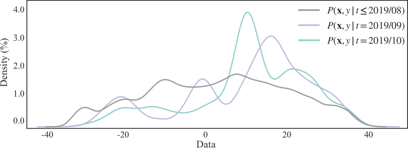
(a) Gradual shift

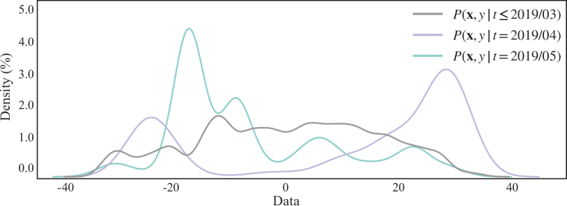
(b) Abrupt shift

Figure 1. Illustration of distribution shifts in CSI 300 stock set. The vector of each stock including dozens of technical indicators and the corresponding label is mapped via t-SNE (van der Maaten and Hinton, 2008) to a 1-D point on the horizontal axis. We estimate the distributions with a kernel density estimator. We plot the distribution of the incremental data in one month in purple, the distribution of all the previous data in black, and the distribution of the next month’s data in green.

Confronted with this challenge, it is noteworthy that the incremental updates stem from two factors: the incremental data and the initial parameters. Conventional IL blindly inherits the parameters learned in the previous task as initial parameter weights and conducts one-sided model adaptation on raw incremental data. To improve IL against distribution shifts, we propose to strengthen the learning scheme by performing two-fold adaptation, namely data adaptation and model adaptation. The data adaptation aims to close the gap between the distributions of incremental data and test data. For example, biased patterns that only exist in incremental data are equivalent to noise with respect to test data and could be resolved through proper data adaptation. Our model adaptation focuses on learning a good initialization of parameters for each IL task, which can appropriately adapt to incremental data and still retain a degree of robustness to distribution shifts. However, it is intractable to design optimal adaptation for each IL task. A proper choice of adaptation varies by forecast model, dataset, period, degree of distribution shifts, and so on. Hence, we borrow ideas from meta-learning (Finn et al., 2017) to realize the two-fold adaptation, i.e., to automatically find profitable data adaptation without human labor or expertise and to reach a sweet spot between adaptiveness and robustness for model adaptation.

In this work, we propose DoubleAdapt, a meta-learning approach to incremental learning for stock trend forecasting. We introduce two meta-learners, namely data adapter and model adapter, which adapt data towards a locally stationary distribution and equip the model with task-specific parameters that have quickly adapted to the incremental data and still generalize well on the test data. The data adapter contains a multi-head feature adaptation layer and a multi-head label adaptation layer in order to obtain adapted incremental data and adapted test data that are profitable for incremental learning. Specifically, the feature adaptation layer transforms all features from the incremental data and the test data, while the label adaptation layer rectifies labels of the incremental data and its inverse function restores model predictions on the test data. By casting the problem of IL for stock trend forecasting as a sequence of meta-learning tasks, we perform each IL task by solving a bi-level optimization problem: (i) in the lower-level optimization, the parameters of the forecast model are initialized by the model adapter and fine-tuned on the adapted incremental data; (ii) in the upper-level optimization, the meta-learners are optimized by test errors on the adapted test data. Throughout the online inference phase, both the two adapters and the forecast model will be updated continually over new IL tasks.

The main contributions of this work are summarized as follows.

• We propose DoubleAdapt, an end-to-end incremental learning framework for stock trend forecasting, which adapts both the data and the model to cope with distribution shifts in the online environment.

• We formulate each incremental learning task as a bi-level optimization problem. The lower level is the forecast model that is initialized by the model adapter and fine-tuned using the adapted incremental data. The upper level includes the data adapter and the model adapter as two meta-learners that are optimized to minimize the forecast error on the adapted test data.

• We conduct experiments on real-world datasets and demonstrate that DoubleAdapt performs effectively against different kinds of distribution shifts and achieves state-of-the-art predictive performance compared with RR and meta-learning methods. DoubleAdapt also enjoys high efficiency compared with RR methods.

2. Preliminaries

In this section, we will introduce some definitions of our work and formulate the incremental learning problem. We also highlight the challenge of distribution shifts.

Definition 1 (Stock Price Trend). Following (Hu et al., 2018; Xu et al., 2021b, a), we define the stock price trend at date $t$ as the stock price change rate of the next day:

(1) $$y^{(t)}=\frac{Price^{(t+1)}-Price^{(t)}}{Price^{(t)}},$$

where $Price^{(t)}$ is the closing price at date $t$ and could also be the opening price or volume-weighted average price (VWAP).

Let $\mathbf{x}^{(t)}\in\mathbb{R}^{D}$ represent the feature vector of a stock at date $t$, where $D$ is the feature dimension. For example, we can constitute $\mathbf{x}$ with opening price, closing price, and other indicators in recent days. Its stock price trend $y$ is the corresponding label. Suppose the stock market comprises $S$ stocks. The collection of features and labels of the $S$ stocks at date $t$ can be denoted as $\mathbf{X}^{(t)}\in\mathbb{R}^{S\times D}$ and $\mathbf{Y}^{(t)}\in\mathbb{R}^{S}$, respectively. The goal of stock trend forecasting is to learn a forecast model $F$ on historical data $\{(\mathbf{X}^{(t)},\mathbf{Y}^{(t)})\}_{t=1}^{T}$ and then forecast the labels of future data $\{(\mathbf{X}^{(t)},\mathbf{Y}^{(t)})\}_{t=T+1}^{T^{\prime}}$, where $T$ and $T^{\prime}$ are the end time of the historical data and the future data, respectively. The parameters of $F$ are denoted as $\theta$.

In online scenarios, new data are coming over time. Once the ground-truth labels of new samples are obtained, we can update the forecast model to learn new emerging patterns. In this work, we focus on incremental learning (IL) for stock trend forecasting, where we periodically launch IL tasks to update the model only with incremental data, as illustrated in Figure 2 and defined as follows.

Definition 2 (IL Task for Stock Trend Forecasting). Supposing a pretrained forecast model is deployed online at date $T$+$1$, we launch an IL task every $r$ dates, where $r$ is predetermined by practical applications. For the $k$-th IL task at date $T$+$kr$+$1$, we fine-tune the model parameters $\theta^{k-1}$ on incremental data ${\mathcal{D}}^{k}_{\text{train}}$ and predict labels on test data ${\mathcal{D}}^{k}_{\text{test}}$ in the following $r$ dates, where ${\mathcal{D}}_{\text{train}}^{k}=\{(\mathbf{X}^{(t)},\mathbf{Y}^{(t)})\}_{t=T+(k-1)r+1}^{T+kr}$ and ${\mathcal{D}}^{k}_{\text{test}}=\{(\mathbf{X}^{(t)},\mathbf{Y}^{(t)})\}_{t=T+kr+1}^{T+(k+1)r}$. The outputs of the $k$-th task are updated parameters $\theta^{k}$ and predictions $\{\hat{\mathbf{Y}}^{(t)}\}_{i=T+kr+1}^{T+(k+1)r}$. The IL task expects the model to quickly adapt to the incremental data, in order to make precise predictions on future data with similar patterns. We can evaluate the predictions by computing a loss function $\mathcal{L}_{\text{test}}$ on ${\mathcal{D}}^{k}_{\text{test}}$, e.g., mean square error.

Problem Statement. Given a predefined task interval $r$, IL for stock trend forecasting is constituted by a sequence of IL tasks, i.e., $\mathcal{T}=$ $\{({\mathcal{D}}_{\text{train}}^{1},{\mathcal{D}}_{\text{test}}^{1})$, $\ ({\mathcal{D}}_{\text{train}}^{2},{\mathcal{D}}_{\text{test}}^{2})$, $\ \cdots,({\mathcal{D}}_{\text{train}}^{k},{\mathcal{D}}_{\text{test}}^{k}),\cdots\}$. In each task, we update the model parameters, do online inference, and end up with performance evaluation on the ground-truth labels of the test data. The goal of IL is to achieve the best overall performance across all test dates, which can be evaluated by excess annualized returns or other ranking metrics of stock trend forecasting.

Typically, IL holds a strong assumption that a model which fits recent data can perform well on the following data under the same distribution. However, as the stock market is dynamically evolving, its data distribution can easily shift over time. $\mathcal{D}_{\text{train}}^{k}$ and $\mathcal{D}_{\text{test}}^{k}$ are likely to have two different joint distributions, i.e., $\mathcal{P}_{\text{train}}^{k}(\mathbf{x},y)\neq\mathcal{P}_{\text{test}}^{k}(\mathbf{x},y)$, where $\mathcal{P}_{\text{train}}^{k}$ and $\mathcal{P}_{\text{test}}^{k}$ denote the distributions of $\mathcal{D}_{\text{train}}^{k}$ and $\mathcal{D}_{\text{test}}^{k}$, respectively. The distribution shifts can be zoomed into the following two cases (Gama et al., 2014):

• Conditional distribution shift when $\mathcal{P}_{\text{train}}^{k}(y\mid\mathbf{x})\neq\mathcal{P}_{\text{test}}^{k}(y\mid\mathbf{x})$;

• Covariate shift when $\mathcal{P}_{\text{train}}^{k}(\mathbf{x})\neq\mathcal{P}_{\text{test}}^{k}(\mathbf{x})$ and $\mathcal{P}_{\text{train}}^{k}(y\mid\mathbf{x})=\mathcal{P}_{\text{test}}^{k}(y\mid\mathbf{x})$.

In either case, excessive updates on incremental data would incur the overfitting issue while deficient updates may result in an underfit model. Hence, distribution shifts pose challenges to incremental learning for stock trend forecasting.

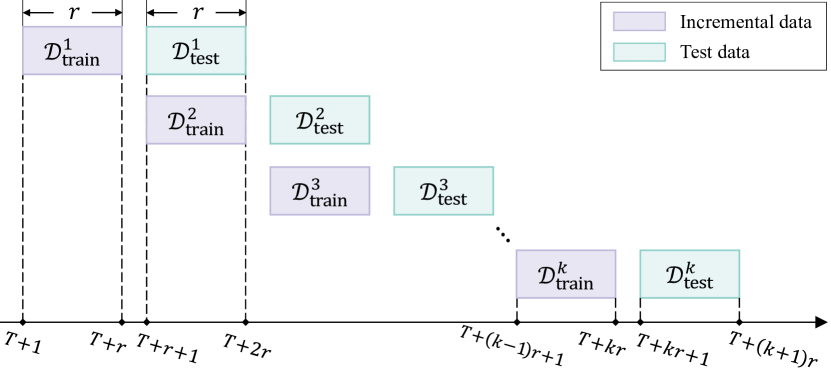
Figure 2. Illustration of IL for stock trend forecasting. $r$ is the timespan of incremental data or test data.

3. Key Insights

To tackle the distribution shift challenge, there are two important directions to follow. One is to close the gap between incremental data and test data so as to perform IL on more stationary distributions. Another is to enhance the generalization ability of the model against distribution shifts. Following both directions, we propose to perform data adaptation and model adaptation for each IL task. We describe our key insights with the following details.

Data Adaptation. A critical yet under-explored direction is to adapt data into a locally stationary distribution so as to mitigate the effects of distribution shifts at the data level. Some RR methods resample all historical data (e.g., 500 million samples) into a new training set that shares a similar distribution with future data (Li et al., 2022). However, such a coarse-grained adaptation fails in IL where incremental data is of limited size (e.g., one thousand samples) and contains deficient samples to reveal future patterns. To address this limitation, we propose to adapt all features and labels of the incremental data to mitigate the effects of distribution shifts in a fine-grained way. We argue that some shift patterns repeatedly appear in the historical data and are learnable. For example, stock prices can overreact to some bullish news and emotional investment, while the prices and the trend patterns tend to shift towards normal in future weeks. Thus, it is often desirable to retract the overreacting features and labels to approach future tendencies. In addition, assuming the original incremental data is reliable, test data of a different distribution can be deemed as a biased dataset. Adapting test data towards the distribution of incremental data has a debiasing effect. Hence, we adapt both $\mathcal{D}_{\text{train}}^{k}$ and $\mathcal{D}_{\text{test}}^{k}$ so as to narrow the gap between their distributions.

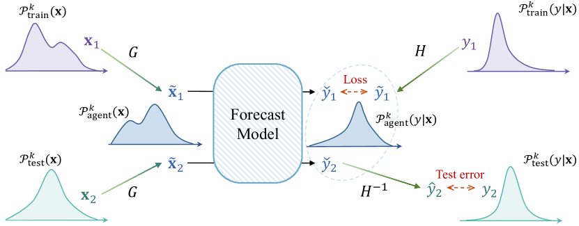
Figure 3. Illustration of data adaptation. The function $G$ adapts the feature distributions of the incremental data and the test data to an agent feature distribution. Similarly, the function $H$ adapts the two posterior distributions to an agent one. Its inverse function $H^{-1}$ restores the model outputs to the original posterior distribution of the test data.

Technically, we cannot directly align $\mathcal{P}_{\text{train}}^{k}(\mathbf{x},y)$ and $\mathcal{P}_{\text{test}}^{k}(\mathbf{x},y)$ because labels of test data are unknown at the inference time. We thus decouple distribution shifts into covariate shifts and conditional distribution shifts, and address them separately, as illustrated in Figure 3. First, we require a mapping function $G$ to transform the features of $\mathcal{D}_{\text{train}}^{k}$ and $\mathcal{D}_{\text{test}}^{k}$ in a fine-grained way, and we expect $G$ to adapt $\mathcal{P}_{\text{train}}^{k}(\mathbf{x})$ and $\mathcal{P}_{\text{test}}^{k}(\mathbf{x})$ to an agent feature distribution $\mathcal{P}_{\text{agent}}^{k}(\mathbf{x})$, alleviating covariate shifts. Second, we apply another mapping function $H$ to adapt the labels of $\mathcal{D}_{\text{train}}^{k}$. We expect $H$ to adapt $\mathcal{P}_{\text{train}}^{k}(y|\mathbf{x})$ to a possible future distribution $\mathcal{P}_{\text{agent}}^{k}(y|\mathbf{x})$, dealing with conditional distribution shifts. Ideally, $H$ could project the labels from $\mathcal{P}_{\text{test}}^{k}(y|\mathbf{x})$ into $\mathcal{P}_{\text{agent}}^{k}(y|\mathbf{x})$ so that a forecast model fitting $\mathcal{P}_{\text{agent}}^{k}(y|\mathbf{x})$ can precisely predict the adapted label for the test data. Finally, we need to inversely map the model outputs from $\mathcal{P}_{\text{agent}}^{k}(y|\mathbf{x})$ to $\mathcal{P}_{\text{test}}^{k}(y|\mathbf{x})$. As such, we narrow the gap between $\mathcal{P}_{\text{train}}^{k}(\mathbf{x})$ and $\mathcal{P}_{\text{test}}^{k}(\mathbf{x})$ via feature adaptation, and narrow the gap between $\mathcal{P}_{\text{train}}^{k}(y|\mathbf{x})$ and $\mathcal{P}_{\text{test}}^{k}(y|\mathbf{x})$ via label adaptation. This allows us to reduce the discrepancy between the joint distributions, alleviating the distribution shift issue.

Model Adaptation. Typically, IL initializes the model by the parameters learned in the previous task and updates the initial parameters on incremental data. Distribution shifts would hinder the test performance if the parameters after updates fall into a local optimum and overfit the incremental data. This motivates us to learn a good initialization of parameters for each IL task. On the one hand, the initial parameters of each task is required to preserve historical experience and retain generalization ability against distribution shifts. On the other hand, the parameters in IL still need to effectively memorize task-specific information without being trapped in past experiences. Therefore, we emphasize another important direction where we optimize the initial parameters of each IL task for robustness and adaptiveness.

Optimization via Meta-learning. Following our key insights, we aim to mitigate distribution shifts at the data level and enhance generalization ability at the parameter level. Desirable data adaptation should make the distributions of the two datasets more similar but still informative for stock trend forecasting. Nevertheless, it is infeasible to manually design proper data adaptation as numerous factors should be considered, e.g., forecast models, datasets, prediction time, degrees of distribution shifts, and so on. For model adaptation, it is also tough to reach a sweet spot between robustness and adaptiveness. We thus introduce a meta-learning optimization objective to guide profitable data adaptation and parameter initialization. Though some normalization techniques  (Du et al., 2021b; Ulyanov et al., 2016; Bronskill et al., 2020) in meta-learning can reduce distribution divergences, they may destroy the original statistical indicators (i.e., mean and standard deviation), which are critical task-specific information and deserve memorization in the online settings. In light of this, we pioneer mitigating the distribution shifts in meta-learning through neural networks rather than normalization.

4. Methodology

4.1. Overview

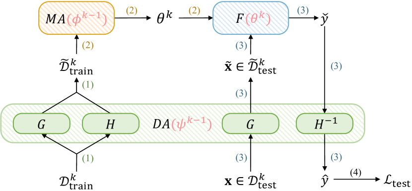
Figure 4. Overview of DoubleAdapt with a data adapter ${DA}$ and a model adapter ${MA}$. The parameters are shown in red.

Figure 4 depicts the overview of our DoubleAdapt framework, which consists of three key components: forecast model $F$ with parameters $\theta$, model adapter ${MA}$ with parameters $\phi$, and data adapter ${DA}$ with parameters $\psi$. $DA$ contains a feature adaptation layer $G$ and a label adaptation layer $H$, along with its inverse function $H^{-1}$. In particular, the implementation of $F$ can be realized by any neural network for stock trend forecasting, such as GRU (Chung et al., 2014) and ALSTM (Qin et al., 2017).

We cast IL for stock trend forecasting as a sequence of meta-learning tasks. For each task $(\mathcal{D}_{\text{train}}^{k},\mathcal{D}_{\text{test}}^{k})$, DoubleAdapt involves four steps as listed below.

1. Incremental data adaptation. Given incremental data $\mathcal{D}_{\text{train}}^{k}$, ${DA}$ transforms each feature vector $\mathbf{x}$ via $G$ and transforms the corresponding label $y$ via $H$, generating an adapted incremental dataset $\mathcal{\widetilde{D}}_{\text{train}}^{k}$.

2. Model adaptation. ${MA}$ initializes the forecast model by parameter weights $\phi^{k-1}$. Following typical IL, we fine-tune the forecast model on $\widetilde{\mathcal{D}}_{\text{train}}^{k}$, generating task-specific parameters $\theta^{k}$. Then, the updated forecast model $F(\cdot;{\theta^{k}})$ is deployed online.

3. Online inference. Given $\mathbf{x}$ of each sample in $\mathcal{D}_{\text{test}}^{k}$, $DA$ transforms it via $G$ into $\tilde{\mathbf{x}}$. Then, $F(\cdot;{\theta^{k}})$ takes $\tilde{\mathbf{x}}$ and produces an intermediate prediction $\check{y}$ which will be transformed via $H^{-1}$ into the final prediction $\hat{y}$. We denote the adapted test dataset by $\mathcal{\widetilde{D}}_{\text{test}}^{k}$ that is obtained by transforming raw features in $\mathcal{D}_{\text{test}}^{k}$.

4. Optimization of meta-learners. We calculate the final forecast error $\mathcal{L}_{\text{test}}$ once we obtain all ground-truth labels in order to optimize our meta-learners (i.e., ${DA}$ and ${MA}$) in the upper level. The parameters of meta-learners are updated from $\phi^{k-1}$ and $\psi^{k-1}$ to $\phi^{k}$ and $\psi^{k}$, which are used for the next IL task.

The meta-learning process is essentially a bi-level optimization problem, where the fine-tuning in Step (2) is the lower-level optimization and Step (4) is the upper-level optimization. Formally, since we desire a minimal forecast error on $\mathcal{\widetilde{D}}_{\text{test}}^{k}$, the bi-level optimization of the $k$-th IL task is defined as

(2) $$\phi^{k},\psi^{k}=\underset{{\phi,\psi}}{\arg\min}\mathcal{L}_{\text{test}}(\mathcal{\widetilde{D}}_{\text{test}}^{k};\theta^{k}),$$

(3) $$\text{s.t.}\quad{\theta}^{k}={MA}(\mathcal{\widetilde{D}}_{\text{train}}^{k};\phi^{k-1}),$$

where

(4) $$\mathcal{\widetilde{D}}_{\text{train }}^{k}={DA}({\mathcal{D}}_{\text{train }}^{k};\psi^{k-1});\quad\mathcal{\widetilde{D}}_{\text{test}}^{k}={DA}({\mathcal{D}}_{\text{test}}^{k};\psi^{k-1}).$$

Note that we only adapt features of ${\mathcal{D}}_{\text{test}}^{k}$ because test labels are unknown during online inference time.

Generally, the best incremental learning algorithm should lead to minimum accumulated errors on all test datasets throughout online inference. However, in the context of stock trend forecasting, we only focus on improving the test performance of the current task since past predictions cannot be withdrawn and future datasets are unseen. Therefore, we greedily optimize $\phi$ and $\psi$ task by task in a practical scenario. Furthermore, we approximate Eq. (2) by one-step gradient descent for the concern of training efficiency.

In the following subsections, we elaborate the two adapters and detail our upper-level optimization.

4.2. Data Adapter

Data adapter ${DA}$ is a meta-learner to learn what data adaptation is favorable for appropriate updates and promising test performance. ${DA}$ consists of three mapping functions, i.e., feature adaptation $G$, label adaptation $H$, and its inverse mapping $H^{-1}$.

Following our insights, we propose a mapping function $G$ to map $\mathcal{P}_{\text{train}}^{k}(\mathbf{x})$ and $\mathcal{P}_{\text{test}}^{k}(\mathbf{x})$ into an agent feature distribution $\mathcal{P}_{\text{agent}}^{k}(\mathbf{x})$, alleviating covariate shifts. We intuitively introduce a dense layer as a simple implementation of ${G}$, which is defined as follows:

(5) $$\tilde{\mathbf{x}}=\mathbf{W}\mathbf{x}+\mathbf{b},$$

where $\tilde{\mathbf{x}}$ denotes the adapted feature vector, $\mathbf{W}\in\mathbb{R}^{D\times D}$ is the parameter matrix, and $\mathbf{b}\in\mathbb{R}^{D}$ is the bias vector. Features from ${\mathcal{D}}_{\text{train }}^{k}$ and ${\mathcal{D}}_{\text{test}}^{k}$ are thereby transformed onto a new common hyperplane via the same affine transformation.

The remaining concern is that one simple dense layer is not expressive enough. Different types of feature vectors may require different transformations, for example, abnormal values need to be scaled or masked, trustworthy features just need identity mapping, and profitable signals need to be emphasized. Moreover, stock price trends tend to bear similar shift patterns when the stocks belong to the same concept (e.g., sector, industry, and business), and vice versa. Accordingly, an appealing solution is to employ different transformation heads and decide which candidate head is more suitable for the input. We thus propose a multi-head feature adaptation layer with multiple feature transformation heads, which is formally defined as follows:

(6) $$\mathbf{\tilde{x}}=G(\mathbf{x}):=\mathbf{x}+\sum_{i=1}^{N}s_{i}\cdot g_{i}(\mathbf{x}),$$

where we add a residual connection (He et al., 2016) in case excessive transformation forgets most raw information; $N$ is the number of heads; $g_{i}$ is the $i$-th feature transformation head; $s_{i}$ is a normalized confidence score to decide the strength of the $i$-th transformation. We implement each $g_{i}$ by a simple dense layer:

(7) $$g_{i}(\mathbf{x})=\mathbf{W}_{i}\mathbf{x}+\mathbf{b}_{i},$$

where $\mathbf{W}_{i}$ and $\mathbf{b}_{i}$ are head-specific transformation parameters. As for confidence estimation, we use $N$ prototype vectors to prompt which head is more applicable. Specifically, we first calculate the cosine similarity $\hat{s}_{i}$ between the feature vector and each prototype, which is formulated as:

(8) $$\hat{s}_{i}=\frac{\mathbf{p}_{i}^{\top}\mathbf{x}}{\|\mathbf{p}_{i}\|\|\mathbf{x}\|},$$

where $\mathbf{p}_{i}\in\mathbb{R}^{D}$ is the $i$-th prototype vector. Then, we derive the normalized score $s_{i}$ by

(9) $$s_{i}=\frac{\exp\hat{s}_{i}/\tau}{\sum_{j=1}^{N}\exp\hat{s}_{j}/\tau},$$

where $\tau$ is a positive hyperparameter to control softmax temperature. With the prototypes deemed as learnable embeddings of hidden concepts in the stock market, the multi-head feature adaptation layer can provide concept-oriented transformations for each input feature vector $\mathbf{x}$.

To cope with conditional distribution shifts, we adapt labels of $\mathcal{D}_{\text{train}}^{k}$. We define a label transformation head as follows:

(10) $$h_{i}(y)={\gamma}_{i}y+\beta_{i},$$

where ${\gamma}_{i}\in\mathbb{R}$ and $\beta_{i}\in\mathbb{R}$ are learnable meta-parameters. A multi-head label adaptation layer, termed as $H$, is formulated as

(11) $$\tilde{y}=H(y):=\sum_{i=1}^{N}s_{i}\cdot h_{i}(y),$$

where $\tilde{y}$ denotes the adapted label; $s_{i}$ has been calculated in the feature adaptation layer and is determined by $\mathbf{x}$.

During online inference, we need to inversely map the intermediate output $\check{y}$ from $\mathcal{P}_{\text{agent}}^{k}(y|\mathbf{x})$ to $\mathcal{P}_{\text{test}}^{k}(y|\mathbf{x})$, where $\check{y}=F(\mathbf{x})$. We define the inverse mapping function $H^{-1}$ by

(12) $$\hat{y}=H^{-1}(\mathbf{x},\check{y}):=\sum_{i=1}^{N}s_{i}\cdot h^{-1}_{i}(\check{y}),$$

where

(13) $$h_{i}^{-1}(\check{y})=({\check{y}-\beta_{i}})/{\gamma_{i}}.$$

One can seek further improvements on the implementation of each label adaptation head $h_{i}$ by various normalizing flows (Kobyzev et al., 2021), which comprise a sequence of invertible mappings. Empirically, we show that the simple linear heads have already been effective in Sec. 6.3.

To summarize, meta-parameters $\psi$ of the data adapter ${DA}$ include the parameters of $G$ and $H$, i.e., $\psi=\{\mathbf{W}_{i},\mathbf{b}_{i},\mathbf{p}_{i},\gamma_{i},\beta_{i}\}_{i=1}^{N}$. The data adapter transforms features of $\mathcal{D}_{\text{train}}^{k}$ and $\mathcal{D}_{\text{test}}^{k}$ by Eq. (6), and transforms labels of $\mathcal{D}_{\text{train}}^{k}$ by Eq. (11). The adapted datasets $\mathcal{\widetilde{D}}_{\text{train}}^{k}$ and $\mathcal{\widetilde{D}}_{\text{test}}^{k}$ in Eq. (4) can be formalized as

(14a) $$\mathcal{\widetilde{D}}_{\text{train}}^{k} =\{(G(\mathbf{x}),H(\mathbf{x},y))\mid(\mathbf{x},y)\in\mathcal{D}_{\text{train }}^{k}\},$$

(14b) $$\mathcal{\widetilde{D}}_{\text{test }}^{k} =\{(G(\mathbf{x}),y)\mid(\mathbf{x},y)\in\mathcal{D}_{\text{test}}^{k}\},$$

where the ground-truth labels in $\mathcal{\widetilde{D}}_{\text{test}}^{k}$ are known at the corresponding trading dates in the future.

4.3. Model Adapter

Model adapter ${MA}$ is another meta-learner to provide a good initialization of model parameters for each IL task and then adapt the initial parameters to fit the incremental data. For the $k$-th IL task, ${MA}$ first assigns the forecast model $F$ with initial weights $\phi^{k-1}$, and then fine-tunes $F({\cdot;\phi^{k-1}})$ on $\mathcal{\widetilde{D}}_{\text{train}}^{k}$. The optimization objective is to reduce the training loss $\mathcal{L}_{\text{train}}$ which is defined as:

(15) $$\mathcal{L}_{\text{train}}=\frac{1}{|\mathcal{\widetilde{D}}_{\text{train}}^{k}|}\sum_{(\tilde{\mathbf{x}},\tilde{y})\in\mathcal{\widetilde{D}}_{\text{train}}^{k}}\left(F(\tilde{\mathbf{x}};\phi^{k-1})-\tilde{y}\right)^{2}.$$

We adapt the initial parameters $\phi^{k-1}$ and derive task-specific parameters $\theta^{k}$ as follows:

(16) $${\theta}^{k} ={MA}(\mathcal{\widetilde{D}}_{\text{train}}^{k};\phi^{k-1})$$

$$=\phi^{k-1}-\eta_{\theta}\nabla_{\phi}\mathcal{L}_{\text{train}}(\mathcal{\widetilde{D}}_{\text{train}}^{k};\phi^{k-1}),$$

where $\eta_{\theta}$ is the learning rate of the forecast model and we only perform one-step gradient updates for fast adaptation. Next, we deploy $F(\cdot;{\theta^{k}})$ online to make predictions on adapted test data $\mathcal{\widetilde{D}}_{\text{test}}^{k}$.

Note that DoubleAdapt is a generic framework for any implementation of the model adapter. The one-step gradient update can also be replaced by other model adaptation approaches, such as context-dependent gating (Masse et al., 2018) and transfer network (Zhang et al., 2020).

4.4. Optimization of Meta-learners

At each test time, we can calculate the test error once the ground-truth labels of the test data are known. Formally, we obtain mean square error $\mathcal{L}_{\text{MSE}}$ to optimize our meta-learners before we start the next task, which is defined as follows:

(17) $$\mathcal{L}_{\text{MSE}}=\frac{1}{|\mathcal{\widetilde{D}}_{\text{test}}^{k}|}\sum_{(\tilde{\mathbf{x}},y)\in\mathcal{\widetilde{D}}_{\text{test}}^{k}}\left(H^{-1}\circ F(\tilde{\mathbf{x}};\theta^{k},\psi^{k-1})-y\right)^{2}.$$

Additionally, we add a regularization term to avoid the adapted labels of $\mathcal{\widetilde{D}}_{\text{train}}^{k}$ being abnormal and hard to learn. We formulate the regularization loss $\mathcal{L}_{\text{reg}}$ by

(18) $$\mathcal{L}_{\text{reg}}=\frac{1}{|\mathcal{D}_{\text{train}}^{k}|}\sum_{(\mathbf{x},y)\in\mathcal{D}_{\text{train}}^{k}}\left(H(\mathbf{\tilde{x}},y;\psi^{k-1})-y\right)^{2}.$$

The final test loss $\mathcal{L}_{\text{test}}$ is derived by

(19) $$\mathcal{L}_{\text{test}}=\mathcal{L}_{\text{MSE}}+\alpha\mathcal{L}_{\text{reg}},$$

where $\alpha$ is a hyperparameter to control the regularization strength. Actually, $\alpha\mathcal{L}_{\text{reg}}$ approximates the second-order gradients of the label adaptation layer (see derivations in Appendix  C.2).

The optimization of our model adapter ${MA}$ is formulated as:

(20) $${\phi}^{k}={\phi}^{k-1}-\eta_{\phi}\nabla_{\phi}\mathcal{L}_{\text{test}}(\mathcal{\widetilde{D}}_{\text{test}}^{k};\theta^{k}),$$

where $\eta_{\phi}$ is the learning rate of ${MA}$. The difference between traditional MAML (Finn et al., 2017) and our method lies in that we only use one query set at each time to update the meta-learner. We are devoted to improving performance on the current test data because the stock market evolves and a large proportion of past data may not contain patterns that will reappear in the future. It is also practical in the IL setting where we only save samples of one task in memory.

Similarly, we optimize ${DA}$ according to actual test performance, using the following equation:

(21) $${\psi}^{k}={\psi}^{k-1}-\eta_{\psi}\nabla_{\psi}\mathcal{L}_{\text{test}}(\mathcal{\widetilde{D}}_{\text{test}}^{k};\theta^{k}),$$

where $\eta_{\psi}$ is the learning rate of ${DA}$. $\mathcal{\widetilde{D}}_{\text{test}}^{k}$ and $\theta^{k}$ are derived by Eq. (14a) and Eq. (16), respectively.

5. Training Procedure

In this section, we propose a two-phase training procedure of DoubleAdapt including an offline training phase and an online training phase. Pseudo-codes are shown in Alg. 1 and Alg. 2.

Input: Meta-train set $\mathcal{T}_{\text{train}}=\{(\mathcal{D}_{\text{train }}^{k},\mathcal{D}_{\text{test}}^{k})\}_{k=1}^{K_{0}}$, meta-valid set $\mathcal{T}_{\text{valid}}=\{(\mathcal{D}_{\text{train }}^{k},\mathcal{D}_{\text{test}}^{k})\}_{k=K_{0}+1}^{K}$ and meta-test set $\mathcal{T}_{\text{test}}=\{(\mathcal{D}_{\text{train }}^{k},\mathcal{D}_{\text{test}}^{k})\}_{k=K+1}^{K^{\prime}}$

Output: Trained parameters $\phi$, $\psi$ and online predictions $\{\mathbf{\hat{Y}}^{(t)}\}_{t=T+1}^{T^{\prime}}$

1

2Initialize $\phi$ and $\psi$;

3

/* Offline training phase */

4 repeat

5       $\mathcal{T}_{\text{train}}^{\prime}\leftarrow\mathtt{shuffle}(\mathcal{T}_{\text{train}})$;

6       $\phi$, $\psi$, $\{\hat{\mathbf{Y}}^{(t)}\}_{\scriptscriptstyle t=r+1}^{\scriptscriptstyle(K_{0}+1)r}$$\leftarrow\mathtt{{DoubleAdapt}}(\phi,\psi,\mathcal{T}_{\text{train}}^{\prime})$;

7       ${\phi^{\prime}}$, ${\psi^{\prime}}\leftarrow$ make a temporary copy of $\phi$ and $\psi$;

8       ${\phi^{\prime}}$, ${\psi^{\prime}}$, $\{\hat{\mathbf{Y}}^{(t)}\}_{\scriptscriptstyle t=(K_{0}+1)r+1}^{\scriptscriptstyle(K+1)r}$$\leftarrow\mathtt{{DoubleAdapt}}({\phi^{\prime}},{\psi^{\prime}},\mathcal{T}_{\text{valid}})$;

9       Calculate metric on $\{\hat{\mathbf{Y}}^{(t)},{\mathbf{Y}}^{(t)}\}_{\scriptscriptstyle t=(K_{0}+1)r+1}^{\scriptscriptstyle(K+1)r}$;

10      

11until the metric decreases for $\zeta$ epochs;

/* Online training phase from $T+1$ to $T^{\prime}$ */

12 $\phi$, $\psi$, $\{\hat{\mathbf{Y}}^{(t)}\}_{\scriptscriptstyle t=H+(K+1)r}^{\scriptscriptstyle T^{\prime}}$$\leftarrow\mathtt{{DoubleAdapt}}(\phi,\psi,\mathcal{T}_{\text{valid}}\cup\mathcal{T}_{\text{test}})$;

13 Evaluate DoubleAdapt by metric on $\{\hat{\mathbf{Y}}^{(t)},{\mathbf{Y}}^{(t)}\}_{t=T+1}^{T^{\prime}}$;

14

return $\phi$, $\psi$, $\{\hat{\mathbf{Y}}^{(t)}\}_{t=T+1}^{T^{\prime}}$

Algorithm 1 Overall training procedure

Input: $\phi$, $\psi$ and task set $\mathcal{T}=\{(\mathcal{D}_{\text{train }}^{k},\mathcal{D}_{\text{test}}^{k})\}_{k=m}^{n}$

Output: $\phi^{n}$, $\psi^{n}$ and predictions $\{\hat{\mathbf{Y}}^{(t)}\}_{t=mr+1}^{(n+1)r}$

1

2$\phi^{(m-1)},\psi^{(m-1)}\leftarrow\phi$, $\psi$;

3 for $k\leftarrow m$ to $n$ do

4       Assign forecast model $F$ with inital weights $\phi^{k-1}$;

5      

6      Predict on $\widetilde{\mathcal{D}}_{\text{train }}^{k}$ defined by Eq. (14a);

7      

8      Compute training loss by Eq. (15);

9      

10      Adapt the forecast model parameters by:

$${\theta}^{k}=\phi^{k-1}-\eta_{\theta}\nabla_{\phi}\mathcal{L}_{\text{train}}(\mathcal{\widetilde{D}}_{\text{train}}^{k};\phi^{k-1});\quad$$

11      $\{\hat{\mathbf{Y}}^{(t)}\}_{t=kr+1}^{(k+1)r}$$\leftarrow$ Predict on $\widetilde{\mathcal{D}}_{\text{test}}^{k}$ defined by Eq. (14b)

12      Compute test loss by Eq. (19);

13      

14      Update data adapter ${DA}$ and model adapter ${MA}$:

$${\psi}^{k}={\psi}^{k-1}-\eta_{\psi}\nabla_{\psi}\mathcal{L}_{\text{test}}(\mathcal{\widetilde{D}}_{\text{test}}^{k};\theta^{k}),\quad\quad\quad$$

$${\phi}^{k}={\phi}^{k-1}-\eta_{\phi}\nabla_{\phi}\mathcal{L}_{\text{test}}(\mathcal{\widetilde{D}}_{\text{test}}^{k};\theta^{k}).\quad\quad\quad$$

15 end for

return $\phi^{n}$, $\psi^{n}$, $\{\hat{\mathbf{Y}}^{(t)}\}_{t=mr+1}^{(n+1)r}$

Algorithm 2 DoubleAdapt

Given all historical data $\{(\mathbf{X}^{(t)},\mathbf{Y}^{(t)})\}_{t=1}^{T}$ before deployment, we organize these offline data into $K$ incremental learning tasks to imitate online incremental learning. The $k$-th IL task consists of the $k$-th incremental data $\mathcal{D}_{\text{train}}^{k}=\{(\mathbf{X}^{(t)},\mathbf{Y}^{(t)})\}_{t=(k-1)r+1}^{kr}$ and the $k$-th test data $\mathcal{D}_{\text{test}}^{k}=\{(\mathbf{X}^{(t)},\mathbf{Y}^{(t)})\}_{t=kr+1}^{(k+1)r}$. We take the first $K_{0}$ tasks as meta-train set $\mathcal{T}_{\text{train}}$ and others as meta-valid set $\mathcal{T}_{\text{valid}}$. It is noteworthy that we can shuffle $\mathcal{T}_{\text{train}}$ to simulate arbitrary distribution shifts in pursuit of robustness against extreme non-stationarity.

Offline training. We pretrain the two meta-learners on $\mathcal{T}_{\text{train}}$ task by task for epochs. At the end of each epoch, we continue incremental learning on $\mathcal{T}_{\text{valid}}$ for evaluation (Alg. 1, L1). The updates of the meta-learners on the meta-valid set are conducted on a temporary copy of the meta-learners (Alg. 1, L1), in order to avoid information leakage. We perform early stopping when the evaluation metric on $\mathcal{T}_{\text{valid}}$ decreases for $\zeta$ consecutive epochs, in order to avoid overfitting. The meta-learners get ready for online service after they have been incrementally updated on the whole validation set (Alg. 1, L1).

Online training. We deploy DoubleAdapt online at date $T$ and incrementally update the meta-learners at the end of each online task (Alg. 2, L2). As a special case, the meta-learners could keep the original adaptation ability of traditional MAML when the learning rates $\eta_{\psi}$ and $\eta_{\phi}$ are always set to zero during the online training phase. However, as the stock market is dynamically evolving, it is critical to continually consolidate the meta-learners with new knowledge, which is also empirically confirmed by our experimental results in Appendix B.

In case the meta-learners encounter the catastrophic forgetting problem, we can also restart offline training after a much larger interval. For example, we incrementally update the meta-learners every week and fully retrain them on an enlarged meta-train set after one-year incremental learning. Integrating the advantages of IL and RR, DoubleAdapt is expected to achieve better performance. In this work, we focus on improving IL performance against distribution shifts and leave the combination of DoubleAdapt and RR as future work. According to our experiments on two real-world stock datasets, DoubleAdapt alone can outperform RR methods for a long period (e.g., over 2.5 years) and hence it is unnecessary to frequently perform full retraining.

Complexity analysis. When optimizing the meta-learners (Alg. 2, L2), we adopt the first-order approximation version of MAML  (Finn et al., 2017) to avoid the expensive computation of Hessian matrices. Therefore, both the time and memory costs per IL task are linearly proportional to the size of incremental data. Formally, let $S$ denote the number of stocks in the market and $E$ denote the number of training epochs for RR methods till convergence. For the $k$-th online task, both the incremental data and the test data have $rS$ samples, while RR takes $(T+kr)S$ historical samples to train the model from scratch. Hence, the time complexity of DoubleAdapt and RR is $O(rS)$ and $O(E(T+kr)S)$, respectively. The scalability of DoubleAdapt allows frequent updates on the forecast model, e.g., on a weekly basis.

6. Experiments

In this section, we study our DoubleAdapt framework with experiments, aiming to answer the following research questions:

• RQ1: How does our proposed DoubleAdapt approach perform compared with the state-of-the-art methods?

• RQ2: How is the effect of different components in DoubleAdapt?

• RQ3: What is the empirical time cost of DoubleAdapt?

An additional hyperparameter study is provided in Appendix B.

6.1. Experimental Settings

6.1.1. Datasets

We evaluate our DoubleAdapt framework on two popular real-world stock sets: CSI 300 (Xu et al., 2021b; Yoo et al., 2021; Hou et al., 2021; Xu et al., 2021a) and CSI 500 (Xu et al., 2021b; Li et al., 2022) in the China A-share market. CSI 300 consists of the 300 largest stocks, reflecting the overall performance of the market. CSI 500 comprises the largest remaining 500 stocks after excluding the CSI 300 constituents, reflecting the small-mid cap stocks.

We use the stock features of Alpha360 in the open-source quantitative investment platform Qlib (Yang et al., 2020). Alpha360 contains 6 indicators on each day, which are opening price, closing price, highest price, lowest price, volume weighted average price (VWAP) and trading volume. For each stock at date $t$, Alpha360 looks back 60 days to construct a 360-dimensional vector as the raw feature of this stock. We use the stock price trend defined in Definition 2 as the label for each stock. Following Qlib, we split stock data into training set (from 01/01/2008 to 12/31/2014), validation set (from 01/01/2015 to 12/31/2016), and test set (from 01/01/2017 to 07/31/2020). The features are normalized by moments of the whole training set, and the labels grouped by date are normalized by moments of data at the same date (Xu et al., 2021b, a).

6.1.2. Evaluation Metrics

We use four widely-used evaluation metrics: IC (Lin et al., 2021), ICIR (Du et al., 2021a), Rank IC (Li et al., 2019), and Rank ICIR (Xu et al., 2021a). At each date $t$, $IC^{(t)}$ could be measured by

(22) $$IC^{(t)}=\frac{1}{N}\frac{(\hat{\mathbf{Y}}^{(t)}-mean(\hat{\mathbf{Y}}^{(t)}))^{\top}(\mathbf{Y}^{(t)}-mean(\mathbf{Y}^{(t)}))}{std(\hat{\mathbf{Y}}^{(t)})\cdot std(\mathbf{Y}^{(t)})},$$

where ${\mathbf{Y}^{(t)}}$ are the raw stock price trends and $\hat{\mathbf{Y}}^{(t)}$ are the model predictions at each date. We report the average IC over all test dates. ICIR is calculated by dividing the average by the standard deviation of IC. Rank IC and Rank ICIR are calculated by ranks of labels and ranks of predictions. Besides, we also use two portfolio metrics, including the excess annualized return (Return) and its information ratio (IR). IR is calculated by dividing the excess annualized return by its standard deviation. Our backtest settings adhere to Qlib’s default strategy.

We ran each experiment 10 times and report the average results. For all six metrics, a higher value reflects better performance.

6.1.3. Baseline

We consider two kinds of model-agnostic retraining approaches as the comparison methods:

(1) Rolling retraining methods:

• RR (Li et al., 2022): RR, short for rolling retraining, periodically retrains a model on all available data with equal weights.

• DDG-DA (Li et al., 2022): This method predicts the data distribution of the next time-step sequentially and re-weights all historical samples to generate a training set, of which the distribution is similar to the predicted future distribution.

(2) Incremental learning methods:

• IL: This method is a naïve incremental learning baseline to fine-tune the model only with the recent incremental data by gradient descent (Zinkevich, 2003).

• MetaCoG (He et al., 2019): This method introduces a per-parameter mask to select task-specific parameters according to the context. MetaCoG updates the masks rather than the model parameters to avoid catastrophic forgetting.

• C-MAML (Caccia et al., 2020): This method follows MAML (Finn et al., 2017) to pretrain slow weights that can produce fast weights to accommodate new tasks. At the online time, C-MAML keeps fine-tuning the fast weights until a distribution shift is detected, and then the slow weights are updated and used to initialize new fast weights.

• DoubleAdapt: Our proposed method. DoubleAdapt learns to initialize parameters and, notably, learns to adapt features and labels, alleviating the distribution shift issue.

Note that there are few studies on incremental learning for stock trend forecasting. We borrow MetaCoG and C-MAML from the continual learning problem as IL-based baselines.

6.1.4. Implementation Details

We have made our implementation publicly available. The time interval of two consecutive tasks is 20 trading days (Xu et al., 2021a). The batch size of RR-based methods approximates the number of samples in incremental data, i.e., 5000 for CSI 300 and 8000 for CSI 500. We apply Adam optimizer with an initial learning rate of 0.001 for the forecast model of all baselines, 0.001 for our model adapter, and 0.01 for our data adapter. We perform early stopping when IC decreases for 8 consecutive epochs. The regularization strength $\alpha$ of DoubleAdapt is 0.5. The head number $N$ is 8 and the temperature $\tau$ is 10. Other hyperparameters of the forecast model (e.g., dimension of hidden states) keep the same for a fair comparison. We use the first-order approximation version of MAML (Finn et al., 2017) for all meta-learning methods.

Table 1. Overall performance comparison on CSI 300 and CSI 500, where the bold values are the best results and the underlined values are the most competitive results (RQ1).

Model	Method	CSI 300						CSI 500
		IC	ICIR	RankIC	RankICIR	Return	IR	IC	ICIR	RankIC	RankICIR	Return	IR
Trans- former	RR	0.0449	0.3410	0.0462	0.3670	0.0881	1.0428	0.0452	0.4276	0.0469	0.4732	0.0639	0.9879
	DDG-DA	0.0420	0.3121	0.0441	0.3420	0.0823	1.0018	0.0450	0.4223	0.0465	0.4634	0.0681	1.0353
	IL	0.0431	0.3108	0.0411	0.2944	0.0854	0.9215	0.0428	0.3943	0.0453	0.4475	0.1014	1.5108
	MetaCoG	0.0463	0.3493	0.0434	0.3133	0.0952	0.9921	0.0449	0.4643	0.0469	0.4629	0.1053	0.8945
	C-MAML	0.0479	0.3560	0.0448	0.3405	0.0986	1.0537	0.0477	0.4620	0.0468	0.4861	0.0930	1.4923
	DoubleAdapt	0.0516	0.3889	0.0475	0.3585	0.1041	1.1035	0.0492	0.4653	0.0490	0.4970	0.1330	1.9761
LSTM	RR	0.0592	0.4809	0.0536	0.4526	0.0805	0.9578	0.0642	0.6187	0.0543	0.5742	0.0980	1.5220
	DDG-DA	0.0572	0.4622	0.0528	0.4415	0.0887	1.0583	0.0636	0.6181	0.0540	0.5783	0.1061	1.6673
	IL	0.0594	0.4664	0.0546	0.4362	0.1089	1.2553	0.0576	0.5550	0.0553	0.5660	0.1249	1.8461
	MetaCoG	0.0515	0.4131	0.0505	0.4197	0.1013	1.1133	0.0573	0.5673	0.0549	0.5908	0.1384	2.0546
	C-MAML	0.0568	0.4601	0.0517	0.4381	0.0963	1.1145	0.0582	0.5863	0.0550	0.5898	0.1315	1.9770
	DoubleAdapt	0.0632	0.5126	0.0567	0.4669	0.1117	1.3029	0.0648	0.6331	0.0594	0.6087	0.1496	2.2220
ALSTM	RR	0.0630	0.5084	0.0589	0.4892	0.0947	1.1785	0.0649	0.6331	0.0575	0.6030	0.1211	1.8726
	DDG-DA	0.0609	0.4915	0.0581	0.4823	0.0966	1.2227	0.0645	0.6298	0.0573	0.6029	0.1042	1.6091
	IL	0.0626	0.4762	0.0585	0.4489	0.1171	1.3349	0.0596	0.5705	0.0579	0.5712	0.1501	2.1468
	MetaCoG	0.0581	0.4676	0.0570	0.4695	0.1140	1.3228	0.0576	0.5874	0.0571	0.6086	0.1403	2.0857
	C-MAML	0.0636	0.5064	0.0588	0.4765	0.1085	1.2432	0.0647	0.6490	0.0598	0.6330	0.1644	2.4636
	DoubleAdapt	0.0679	0.5480	0.0594	0.4882	0.1225	1.4717	0.0653	0.6404	0.0607	0.6170	0.1738	2.5192
GRU	RR	0.0629	0.5105	0.0581	0.4856	0.0933	1.1428	0.0669	0.6588	0.0586	0.6232	0.1200	1.8629
	DDG-DA	0.0623	0.5045	0.0589	0.4898	0.0967	1.1606	0.0666	0.6575	0.0582	0.6234	0.1264	1.9963
	IL	0.0633	0.4818	0.0596	0.4609	0.1166	1.3196	0.0637	0.6093	0.0617	0.6291	0.1626	2.3352
	MetaCoG	0.0560	0.4443	0.0545	0.4503	0.0992	1.1014	0.0603	0.5741	0.0585	0.5720	0.1587	2.2635
	C-MAML	0.0638	0.5085	0.0595	0.4865	0.1121	1.3210	0.0646	0.6498	0.0600	0.6494	0.1693	2.5064
	DoubleAdapt	0.0687	0.5497	0.0621	0.5110	0.1296	1.5123	0.0686	0.6652	0.0632	0.6445	0.1748	2.4578

6.2. Performance Comparison (RQ1)

We instantiate the forecast model by four deep neural networks, including Transformer (Vaswani et al., 2017), LSTM (Hochreiter and Schmidhuber, 1997), ALSTM (Qin et al., 2017), and GRU (Chung et al., 2014). Table 1 compares the overall performance of all baselines. Though RR methods are strong baselines and often beat simple IL methods, our proposed DoubleAdapt framework achieves the best results in almost all the cases, demonstrating that DoubleAdapt can make more precise predictions in stock trend forecasting. Exceptionally, C-MAML sometimes achieves higher ICIR or Rank ICIR than DoubleAdapt on CSI 500. During the online training phase, C-MAML modulates the learning rate of its meta-learner according to the test error and thus achieves more stable performance on daily IC. Note that this update modulation is orthogonal to our work and can also be integrated into DoubleAdapt. We also observe that MetaCoG is nearly the worst method that even performs worse than naïve IL. MetaCoG focuses on catastrophic forgetting issues and selectively masks the model parameters, instead of consolidating the parameters with new knowledge acquired online. This observation confirms the significance of online updates for stock trend forecasting. As for the implementation of the forecast model, DoubleAdapt can consistently achieve better performance with a stronger backbone.

Table 2. Ablation study on CSI 300 (RQ2). The forecast model is GRU. The head number $N$ is 8 unless otherwise stated. $IL+{MA}+{DA}$ is our proposed method. The column Overall Performance corresponds to the results on CSI 300 in Table 1.

Method	Overall Performance				Gradual Shifts				Abrupt Shifts
	IC	ICIR	RankIC	RankICIR	IC	ICIR	RankIC	RankICIR	IC	ICIR	RankIC	RankICIR
IL	0.0633	0.4818	0.0596	0.4609	0.0643	0.4936	0.0652	0.5161	0.0690	0.5134	0.0619	0.4581
$+{DA}$	0.0659	0.5279	0.0615	0.4993	0.0708	0.5938	0.0692	0.5897	0.0690	0.5271	0.0620	0.4677
$+{MA}$	0.0658	0.5160	0.0610	0.4910	0.0703	0.5703	0.0680	0.5686	0.0681	0.5085	0.0618	0.4594
$+{MA}$+$G$	0.0678	0.5360	0.0619	0.4978	0.0740	0.6155	0.0709	0.6060	0.0694	0.5224	0.0626	0.4672
$+{MA}$+$H$+$H^{-1}$	0.0660	0.5207	0.0614	0.4995	0.0714	0.5846	0.0701	0.5958	0.0680	0.5093	0.0616	0.4615
$+{MA}$+${DA}$ ($N$=1)	0.0684	0.5462	0.0622	0.5074	0.0744	0.6227	0.0703	0.6029	0.0710	0.5430	0.0634	0.4822
+MA+DA ($\boldsymbol{N}$=8)	0.0687	0.5497	0.0621	0.5110	0.0755	0.6390	0.0713	0.6243	0.0699	0.5323	0.0620	0.4730

6.3. Ablation Study (RQ2)

In this section, we investigate the effects of the key components in DoubleAdapt. Note that IL is also a special case of DoubleAdapt when ${DA}$ always provides identity mappings and $\phi^{k-1}$ is directly updated into $\theta^{k}$ instead of performing gradient descent. We introduce some variants by equipping IL with one or several components. Besides, as the performance varies in different degrees of distribution shifts, we also evaluate the online predictions under different kinds of shifts. To this end, we pretrain the model $F$ on the training set and adopt naïve IL throughout the tasks. In the $k$-th task of the test set, we first use $F$ to do inference on $\mathcal{D}^{k}_{\text{test}}$ without training on $\mathcal{D}^{k}_{\text{train}}$, resulting in a mean square error $\mathcal{L}^{k}_{1}$. Then we update $F$ on $\mathcal{D}^{k}_{\text{train}}$ and infer the same test samples, resulting in a new mean square error $\mathcal{L}^{k}_{2}$. The distribution shift in this task can be measured by $\Delta\mathcal{L}^{k}=\mathcal{L}^{k}_{2}-\mathcal{L}^{k}_{1}$ which can reflect whether $F$ benefits from the incremental update. When $\mathcal{P}^{k}_{\text{test}}$ is similar to $\mathcal{P}^{k}_{\text{train}}$, $\mathcal{L}^{k}_{2}$ should be smaller than $\mathcal{L}^{k}_{1}$, and vice versa. With all online tasks sorted by $\Delta\mathcal{L}^{k}$ in an ascending order, we take the first 25% tasks as cases of gradual shifts and the last 25% tasks as cases of abrupt shifts.

Table 2 shows the average results over the two kinds of distribution shifts on CSI 300, i.e., gradual shifts and abrupt shifts. Applying both ${MA}$ and ${DA}$ into IL, DoubleAdapt achieves the best results against different kinds of distribution shifts. In the cases of gradual shifts, the multi-head version with better expressiveness significantly outperforms the single-head one. Nevertheless, the multi-head version performs worse in the cases of abrupt shifts because its high complexity is a double-edged sword and may incur overfitting issues. As gradual shift is the major issue in stock data (Li et al., 2022), the multi-head version still achieves the best overall performance. Also, it is noteworthy that our proposed data adaptation effectively facilitates model adaptation, and data adaptation alone also beats one-sided model adaptation. On the other hand, the improvement of DoubleAdapt over $IL$+$DA$, especially under abrupt shifts, indicates that the initial parameters of each task are also critical to generalization ability.

Moreover, either the data adaptation or the model adaptation outperforms the most competitive methods (i.e., DDG-DA and C-MAML) in Table 1. Specifically, IL+DA outperforms DDG-DA by 5.6% improvement on IC, and IL+MA outperforms C-MAML by 3.3% improvement on IC. In terms of model adaptation, C-MAML proposes additional modules to deal with catastrophic forgetting in general continual learning problems. However, future stock trends are mainly affected by recent stock trends, and it is more beneficial to learn new patterns from recent data rather than memorize long-term historical patterns. Thus, our simple variant IL+MA achieves better performance than C-MAML.

6.4. Time Cost Study (RQ3)

Table 3. Empirical time cost (in second) comparison.

Model	Method	CSI 300		CSI 500
		Offline	Online	Offline	Online
GRU	RR	-	6064	-	10793
	DDG-DA	1862	6719	2360	10713
	IL	256	58	394	75
	MetaCoG	457	59	784	76
	C-MAML	314	62	533	77
	DoubleAdapt	356	61	677	79

Table 3 compares the total time costs in offline training and online training of different methods. IL methods show superior efficiency compared with RR methods in either offline training or online training. As we adopt the first-order approximation of MAML, we avoid the expensive computation of Hessian matrices. Thus the meta-learning methods are not much slower than naïve IL, and the excess time cost is small enough to omit. It is practical for model selection, hyperparameter tuning, and retraining algorithm selection. Moreover, the low time cost of DoubleAdapt in offline training paves the way for collaboration with RR, e.g., periodically retraining the meta-learners once a year.

7. Related Work

7.1. Stock Trend Forecasting

Profitable quantitative investment usually depends on precise predictions of stock price trends. In recent years, great efforts (Zhang et al., 2017; Li et al., 2018; Zhao et al., 2018; Hu et al., 2018; Yoo et al., 2021; Xu et al., 2021b, a) have been devoted to designing deep-learning approaches to capture intricate finance patterns, while only a few works study online learning for stock data. MASSER (Zhan et al., 2022), which mainly focuses on stock movement prediction in the offline setting, introduces Bayesian Online Changepoint Detection in online experiments to detect distribution shifts and updates its meta-learner after a detection. Such delayed updates can easily lead to inferior performance in online inference. DDG-DA (Li et al., 2022), an advanced RR method, copes with distribution shifts by predicting the future data distribution and resampling the training data for a similar distribution. DDG-DA adapts the training data by assigning samples grouped by periods with different weights before a distribution shift happens. By contrast, our data adaptation transforms the features and the label of each sample in a fine-grained way.

7.2. Meta-Learning

Meta-learning aims to fast adapt to new tasks only with a few training samples, dubbed support set, and generalize well on test samples, dubbed query set. MAML (Finn et al., 2017) is the most widely adopted to learn how to fine-tune for good performance on query sets. Some works (Finn et al., 2019; Nagabandi et al., 2019; He et al., 2020) extend MAML to online settings on the assumption that the support set and the corresponding query set come from the same context, i.e., following the same distribution. As such, the meta-learner will quickly remember task-specific information and perform well on a similar query set. However, this assumption cannot hold when discrepancies between the two sets are non-negligible. LLF (You et al., 2021) studies MAML in an offline setting, proving that a predictor optimized by MAML can generalize well against concept drifts. However, the query sets are unlabeled in online settings, and one can only retrain the meta-learner after detecting a shift (Caccia et al., 2020). Consequently, the predictions are still susceptible to distribution shifts. Some methods (Zhang et al., 2020; You et al., 2022) combine incremental learning and meta-learning for recommender systems and dynamic graphs but ignore distribution shifts. SML (Zhang et al., 2020) focuses on model adaptation and proposes a transfer network to convert model parameters on incremental data, which is orthogonal to our work.

8. Conclusion

In this work, we propose DoubleAdapt, a meta-learning approach to incremental learning for stock trend forecasting. We give two key insights to handle distribution shifts. First, we learn to adapt data into a locally stationary distribution in a fine-grained way. Second, we learn to assign the forecast model with initial parameters which can fast adapt to incremental data and still generalize well against distribution shifts. Experiments on real-world datasets demonstrate that DoubleAdapt is generic and efficient, achieving state-of-the-art predictive performance in stock trend forecasting.

In the future, we will try to combine our incremental learning algorithm and rolling retraining to avoid catastrophic forgetting issues after a long-period online incremental learning. We also believe the idea of the two-fold adaptation can inspire other applications that encounter the challenge of complex distribution shifts.

Appendix A Implementation Details

In practice, we employ shared transformation parameters for all time steps of the features when the stock data are taken as time series. Formally, let $\mathbf{x}=\{x_{1},x_{2},\cdots,x_{L}\}$ represent the stock feature, where $L$ is the length of time series. Each element $x_{j}\in\mathbb{R}^{d}$ is the feature at step $j$, where $d$ is the number of indicators at each time step. The parameters of the $i$-th transformation head is $\mathbf{W}_{i}\in\mathbb{R}^{d\times d}$ and $\mathbf{b}_{i}\in\mathbb{R}^{d}$. At each time step $j$, we first calculate the cosine similarity $\hat{s}_{ij}$ between each pair of $x_{j}$ and $\mathbf{p}_{i}$, where $\mathbf{p}_{i}\in\mathbb{R}^{d}$. Then, we perform softmax operation over the $N$ heads to obtain the confidence score $s_{ij}$. As such, features of $\mathbf{x}$ at all time steps are fed into the shared feature adaptation layer with different scores. It is practical to avoid gradient vanishing issues in RNNs. Otherwise, the gradients of more previous steps are too small to train unshared adaptation parameters.

As for the label adaptation layer, we first employ a linear transformation matrix to cast $\mathbf{x}\in\mathbb{R}^{Ld}$ into a low-dimensional vector $\mathbf{v}$. The confidence score for head selection is calculated by the cosine similarity between $\mathbf{v}$ and $\mathbf{p}^{\prime}_{i}$, where $\mathbf{p}^{\prime}_{i}$ is a specific prototype for label adaptation and has the same dimension with $\mathbf{v}$.

Appendix B Hyperparameter Study

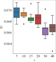
(a) Task interval

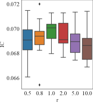
(b) Softmax temparature

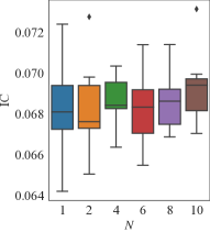
(c) Number of heads

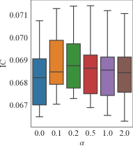
(d) Regularization strength

Figure 5. Performance comparison under different hyperparameters on CSI 300. Outliers are marked in diamonds.

In this section, we evaluate the performance of DoubleAdapt on different values of hyperparameters. We only provide the results on CSI 300 with the forecast model implemented by GRU. The results on CSI 300 are similar.

Task interval $r$. Figure 5(a) shows that more frequent incremental learning with a smaller interval $r$ (e.g., 5 trading days) can lead to better performance. This is because up-to-date patterns are more informative to future trends than previous ones, and it is beneficial to consolidate the forecast model and the meta-learners with new knowledge more timely. It is noteworthy that RR methods with a smaller $r$ will suffer from much more expensive time consumption. In contrast, DoubleAdapt shows superiority in its scalability and is applicable to a small $r$.

Softmax temperature $\tau$. As shown in Figure 5(b), DoubleAdapt achieves the worst performance when we set the softmax temperature $\tau$ to 0.5. We reason that the logits from softmax with a small temperature approximate a one-hot vector, i.e., one sample is transformed by merely one head. Thereby, the adaptation layers are trained by fewer samples and can suffer from underfitting issues. Fortunately, it is always safe to set the temperature with a great value and even towards infinity, since a single-head version of DoubleAdapt still achieves outstanding performance in Table 2.

Number of transformation heads $N$. As shown in Figure 5(c), almost all the multi-head versions of DoubleAdapt outperform the single-head one. Exceptionally, the two-head version shows lower average IC but achieves the highest ceiling value. With a carefully selected temperature (e.g., 1.0), the multi-head version can outperform the single-head one by a larger margin. Note that our incremental learning framework is efficient, and the time cost for hyperparameter tuning is durable. Besides, it is not recommended to use too many heads which can result in more time cost and may also cause overfitting issues.

Regularization strength $\alpha$. Figure 6 shows that DoubleAdapt without regularization achieves inferior performance, which verifies our proposed regularization technique. Nevertheless, the IC performance gradually decreases with a larger regularization strength which hinders the proposed label adaptation. Thus, it is desirable to set moderate regularization to train DoubleAdapt smoothly. Generally, DoubleAdapt is relatively not sensitive to the regularization strength $\alpha$.

Online learning rates $\eta_{\phi}$ and $\eta_{\psi}$. As shown in Figure 5(b), we evaluate the performance on different learning rates of the two meta-learners during the online training phase, while we use the same pretrained meta-learners before online deployment. When we freeze the meta-learners online with both $\eta_{\phi}$ and $\eta_{\psi}$ set to zero, DoubleAdapt achieves the worst results. This confirms that it is critical to continually consolidate the meta-learners with new knowledge acquired online. Nevertheless, DoubleAdapt still keeps the best performance when we freeze the data adapter with a zero $\eta_{\psi}$ but fine-tune the model adapter with an appropriate $\eta_{\phi}$ (0.0005 or 0.001). We conjecture that the pretrained data adapter has learned high-level patterns of distribution shifts, which are shared by the majority of the meta-test set. By contrast, the forecast model should accommodate the up-to-date trends of the stock markets which may not exist in the historical data. This requires the model adapter to be continually fine-tuned on recent incremental data in the online training phase. Otherwise, DoubleAdapt shows inferior performance due to a zero $\eta_{\psi}$, even if we fine-tune the data adapter with a positive $\eta_{\phi}$. Besides, as shown in the rightmost column and the bottom row of Figure 6, the performance degrades with too large learning rates due to catastrophic forgetting issues. It is suggested to tune the hyperparameters of online learning rates on the meta-valid set by using the same pretrained meta-learners for efficiency.

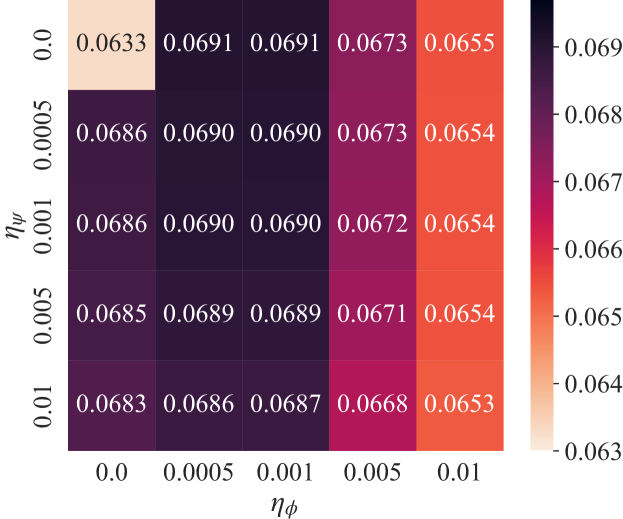
Figure 6. Performance comparison under different online learning rates of the meta-learners on CSI 300. The learning rate $\eta_{\phi}$ of the model adapter varies on the horizontal axis. The learning rate $\eta_{\psi}$ of the data adapter varies on the vertical axis.

Appendix C Approximation of Meta-gradients

Considering efficiency, we apply first-order approximation in the upper-level optimization of the meta-learners, avoiding the expensive computation of high-order gradients.

To simplify notations, we omit the superscript of the parameters in the following derivations, i.e., $\theta$ for $\theta^{k}$, $\phi$ for $\phi^{k-1}$, and $\psi$ for $\psi^{k-1}$. We further distinguish the parameters of the feature adaptation layer and the label adaptation layer as $\psi_{x}$ and $\psi_{y}$, respectively. We also use $\eta$ to represent $\eta_{\theta}$.

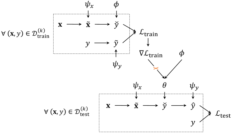
Figure 7. Illustration of our computation graph

C.1. Gradients of Model Adapter

The gradients of $\phi$ can be derived by the chain rule:

(23) $$\nabla_{\phi}\mathcal{L}_{\text{test}}(\theta)= \frac{\partial\mathcal{L}_{\text{test}}(\theta)}{\partial\theta}\frac{\partial\theta}{\partial\phi}$$

$$= \frac{\partial\mathcal{L}_{\text{test}}(\theta)}{\partial\theta}\frac{\partial(\phi-\eta\nabla_{\phi}\mathcal{L}_{\text{train}}(\phi))}{\partial\phi}$$

$$= \frac{\partial\mathcal{L}_{\text{test}}(\theta)}{\partial\theta}\left(1-\eta\frac{\partial}{\partial\phi}\nabla_{\phi}\mathcal{L}_{\text{train}}(\phi)\right)$$

Following MAML (Finn et al., 2017), we assume that the second-order gradient is small enough to omit. Thus, we can derive the first-order approximation by

(24) $$\nabla_{\phi}\mathcal{L}_{\text{test}}(\theta)\approx\frac{\partial\mathcal{L}_{\text{test}}(\theta)}{\partial\theta}=\nabla_{\theta}\mathcal{L}_{\text{test}}(\theta).$$

C.2. Gradients of Data Adapter

As shown in Figure 7, the adaptation on features and predictions in the test data involves first-order gradients which directly optimize $\psi_{x}$ and $\psi_{y}$. Inspired by (Pham et al., 2020), we can also estimate the second-order gradient of $\psi_{y}$ introduced by $\mathcal{L}_{\text{train}}$. As we now focus on the second-order gradient, we leave out the first-order one in $\nabla_{\psi_{y}}\mathcal{L}_{\text{test}}(\theta)$ in the following derivations.

First, we refomulate the task-specific parameter $\theta$ (i.e., $\theta^{k}$) by

(25) $$\theta=\phi-\eta\mathbb{E}_{(\tilde{\mathbf{x}},\tilde{y})\in\mathcal{\widetilde{D}}_{\text{train}}}\nabla_{\phi}\mathcal{L}_{\text{MSE}}(F(\mathbf{\tilde{x}}),\tilde{y}).$$

As $\phi$ is independent of $\psi_{y}$, we derive the second-order gradients of $\psi_{y}$ by

(26) $$\nabla_{\psi_{y}}\mathcal{L}_{\text{test}}(\theta)= \frac{\partial\mathcal{L}_{\text{test}}(\theta)}{\partial\theta}\frac{\partial\theta}{\partial\psi_{y}}$$

$$= \frac{\partial\mathcal{L}_{\text{test}}(\theta)}{\partial\theta}\frac{\partial(\phi-\eta\mathbb{E}_{(\tilde{\mathbf{x}},\tilde{y})\in\mathcal{\widetilde{D}}_{\text{train}}}\nabla_{\phi}\mathcal{L}_{\text{MSE}}(F(\mathbf{\tilde{x}}),\tilde{y}))}{\partial{\psi_{y}}}$$

$$= -\eta\frac{\partial\mathcal{L}_{\text{test}}(\theta)}{\partial\theta}\left(\frac{\partial}{\partial\psi_{y}}\mathbb{E}_{(\tilde{\mathbf{x}},\tilde{y})\in\mathcal{\widetilde{D}}_{\text{train}}}\nabla_{\phi}\mathcal{L}_{\text{MSE}}(F(\mathbf{\tilde{x}}),\tilde{y})\right)$$

Note that $\mathbb{E}_{(\tilde{\mathbf{x}},\tilde{y})\in\mathcal{\widetilde{D}}_{\text{train}}}$ is actually a Monte Carlo approximation of $\mathbb{E}_{(\tilde{\mathbf{x}},\tilde{y})\sim\mathcal{P}_{\text{agent}}(\mathbf{x},y)}$. We have

(27) $$\frac{\partial}{\partial\psi_{y}}\mathbb{E}_{(\tilde{\mathbf{x}},\tilde{y})\in\mathcal{\widetilde{D}}_{\text{train}}}\nabla_{\phi}\mathcal{L}_{\text{MSE}}(F(\mathbf{\tilde{x}}),\tilde{y})$$

$$= \frac{\partial}{\partial\psi_{y}}\mathbb{E}_{(\tilde{\mathbf{x}},\tilde{y})\sim\mathcal{P}_{\text{agent}}(\mathbf{x},y)}\nabla_{\phi}\mathcal{L}_{\text{MSE}}(F(\mathbf{\tilde{x}}),\tilde{y})$$

$$= \mathbb{E}_{\tilde{\mathbf{x}}\sim\mathcal{P}_{\text{agent}}(\mathbf{x})}\frac{\partial}{\partial\psi_{y}}\mathbb{E}_{\tilde{y}\sim\mathcal{P}_{\text{agent}}(y|\mathbf{x})}\nabla_{\phi}\mathcal{L}_{\text{MSE}}(F(\mathbf{\tilde{x}}),\tilde{y})),$$

where we extract the expectation on $\tilde{\mathbf{x}}$ out of the gradient on $\psi_{y}$ as $\tilde{\mathbf{x}}$ is independent of $\psi_{y}$.

Since $\nabla_{\phi}\mathcal{L}_{\text{MSE}}(F(\mathbf{\tilde{x}}),\tilde{y}))$ has no dependency on $\psi_{y}$, except for via $\tilde{y}$, we can apply the REINFORCE rule (Williams, 1992) to achieve

(28) $$\frac{\partial}{\partial\psi_{y}}\mathbb{E}_{\tilde{y}\sim\mathcal{P}_{\text{agent}}(y|\mathbf{x})}\left[\nabla_{\phi}\mathcal{L}_{\text{MSE}}(F(\mathbf{\tilde{x}}),\tilde{y}))\right]$$

$$= \mathbb{E}_{\tilde{y}\sim\mathcal{P}_{\text{agent}}(y|\mathbf{x})}\left[\nabla_{\phi}\mathcal{L}_{\text{MSE}}(F(\mathbf{\tilde{x}}),\tilde{y})\cdot\frac{\partial\log P(\tilde{y}\mid\mathbf{x},y;\psi_{y})}{\partial\psi_{y}}\right],$$

where $P(\tilde{y}\mid\mathbf{x},y;\psi_{y})$ is the probability density of $\mathcal{P}_{\text{agent}}(y|\mathbf{x})$.

Assume the conditional probability follows a normal distribution, i.e., $P(\tilde{y}\mid\mathbf{x},y)=\mathcal{N}(y,\sigma^{2})$, where $\sigma$ is a constant. We have

(29) $$\frac{\partial\log P(\tilde{y}|\mathbf{x},y;\psi_{y})}{\partial\psi_{y}}= \frac{\partial\left(-\frac{1}{2}\log\left(2\pi\sigma^{2}\right)-\frac{1}{2\sigma^{2}}\left(\tilde{y}-y\right)^{2}\right)}{\partial\psi_{y}}$$

$$= \frac{\partial\left(-\frac{1}{2}\log\left(2\pi\sigma^{2}\right)-\frac{1}{2\sigma^{2}}\mathcal{L}_{\text{MSE}}(\tilde{y},y)\right)}{\partial\psi_{y}}$$

$$= -\frac{1}{2\sigma^{2}}\frac{\partial\mathcal{L}_{\text{MSE}}(\tilde{y},y)}{\partial\psi_{y}}$$

Then Eq. (27) becomes

(30) $$\frac{\partial}{\partial\psi_{y}}\mathbb{E}_{(\tilde{\mathbf{x}},\tilde{y})\in\mathcal{\widetilde{D}}_{\text{train}}}\nabla_{\phi}\mathcal{L}_{\text{MSE}}(F(\mathbf{\tilde{x}}),\tilde{y})$$

$$= \frac{-1}{2\sigma^{2}}\mathbb{E}_{\tilde{\mathbf{x}}\sim\mathcal{P}_{\text{agent}}(\mathbf{x})}\mathbb{E}_{\tilde{y}\sim\mathcal{P}_{\text{agent}}(y|\mathbf{x})}\left[\nabla_{\phi}\mathcal{L}_{\text{MSE}}(F(\mathbf{\tilde{x}}),\tilde{y}))\frac{\partial\mathcal{L}_{\text{MSE}}(\tilde{y},y)}{\partial\psi_{y}}\right]$$

$$= \frac{-1}{2\sigma^{2}}\mathbb{E}_{(\tilde{\mathbf{x}},\tilde{y})\in\mathcal{\widetilde{D}}_{\text{train}}}\left[\nabla_{\phi}\mathcal{L}_{\text{MSE}}(F(\mathbf{\tilde{x}}),\tilde{y}))\frac{\partial\mathcal{L}_{\text{MSE}}(\tilde{y},y)}{\partial\psi_{y}}\right]$$

$$= \frac{-1}{2\sigma^{2}}\nabla_{\phi}\mathcal{L}_{\text{train}}(\phi)\frac{\partial\ \mathbb{E}_{(\tilde{\mathbf{x}},\tilde{y})\in\mathcal{\widetilde{D}}_{\text{train}}}\mathcal{L}_{\text{MSE}}(\tilde{y},y)}{\partial\psi_{y}},$$

$$= \frac{-1}{2\sigma^{2}}\nabla_{\phi}\mathcal{L}_{\text{train}}(\phi)\frac{\partial\mathcal{L}_{\text{reg}}}{\partial\psi_{y}},$$

where $\mathcal{L}_{\text{MSE}}(\tilde{y},y)$ is only calculated on the training samples, and the expectation is actually the regularization loss $\mathcal{L}_{\text{reg}}$ in our paper. Then, we substitute Eq. (30) into Eq. (26) to obtain

(31) $$\nabla_{\psi_{y}}\mathcal{L}_{\text{test}}(\theta)=\frac{\eta}{2\sigma^{2}}[\nabla_{\theta}\mathcal{L}_{\text{test}}(\theta)]^{\top}\cdot\nabla_{\phi}\mathcal{L}_{\text{train}}(\phi)\cdot\frac{\partial\mathcal{L}_{\text{reg}}}{\partial\psi_{y}}.$$

With Taylor expansion, we have

(32) $$\mathcal{L}_{\text{test}}(\phi)\approx\mathcal{L}_{\text{test}}(\theta)+[\nabla_{\theta}\mathcal{L}_{\text{test}}(\theta)]^{\top}(\phi-\theta).$$

Note that

(33) $$\theta=\phi-\eta\nabla_{\phi}\mathcal{L}_{\text{train}}(\phi).$$

Thus,

(34) $$\mathcal{L}_{\text{test}}(\phi)-\mathcal{L}_{\text{test}}(\theta)\approx\eta[\nabla_{\theta}\mathcal{L}_{\text{test}}(\theta)]^{\top}\nabla_{\phi}\mathcal{L}_{\text{train}}(\phi)$$

Finally, the second-order gradient of $\psi_{y}$ is approximated by

(35) $$\nabla_{\psi_{y}}\mathcal{L}_{\text{test}}(\theta)=\frac{\mathcal{L}_{\text{test}}(\phi)-\mathcal{L}_{\text{test}}(\theta)}{2\sigma^{2}}\cdot\frac{\partial\mathcal{L}_{\text{reg}}}{\partial\psi_{y}},$$

where we set $\sigma$ as a hyperparameter. Thus the coefficient of gradients by $\mathcal{L}_{\text{reg}}$ is similar to $\alpha$ which controls the regularization strength when $\mathcal{L}_{\text{test}}(\phi)\geq\mathcal{L}_{\text{test}}(\theta)$. If otherwise, the updated parameters result in a greater loss, meaning that the incremental data is noisy and perhaps we should make the adapted labels $\tilde{y}$ more different from the original $y$.