Lightweight Attribute Localizing Models for Pedestrian Attribute Recognition

Abstract

Pedestrian Attribute Recognition (PAR) deals with the problem of identifying features in a pedestrian image. It has found interesting applications in person retrieval, suspect re-identification and soft biometrics. In the past few years, several Deep Neural Networks (DNNs) have been designed to solve the task; however, the developed DNNs predominantly suffer from over-parameterization and high computational complexity. These problems hinder them from being exploited in resource-constrained embedded devices with limited memory and computational capacity. By reducing a network’s layers using effective compression techniques, such as tensor decomposition, neural network compression is an effective method to tackle these problems. We propose novel Lightweight Attribute Localizing Models (LWALM) for Pedestrian Attribute Recognition (PAR). LWALM is a compressed neural network obtained after effective layer-wise compression of the Attribute Localization Model (ALM) using the Canonical Polyadic Decomposition with Error Preserving Correction (CPD-EPC) algorithm.

Convolutional Neural Networks (CNNs) have been used to solve numerous computer vision tasks, such as image recognition, object detection and pose estimation. Although, some of the recent CNN’s show promising results in image recognition, they suffer from high computational complexity and overparameterization. In many cases these problems act as roadblocks for their utilization in power/memory constrained hardware devices such as smartphones and surveillance cameras. Reducing NN’s parameters and computational complexity is an active area of research, and a possibility of reduction without hindering their inference accuracy has been both theoretically and experimentally challenging. There are four known categories of model reduction: low-rank tensor approximation, prunning, quantization and knowledge distillation. In a typical pruning algorithm redundant weights are pruned and important weights are kept. It generally consists of a three-stage pipeline, i.e., training, pruning and fine-tuning which makes it computationally very expensive. Unstructured pruning fails to show runtime speed-up on conventional GPUs, while structured pruning is problematic due to change in NN’s structure. Quantization technique deals with conversion and storing weights at bit widths lower than floating point precision. Therefore, the associated back-propagation becomes infeasible, and the global structure of weights becomes inconvenient to maintain; hence, it makes quantized models hard to converge, and significantly reduces the accuracy. Knowledge Distillation is the process of transferring knowledge from a large model to a smaller one, since large models have higher knowledge capacity than smaller models, there often remains a surprisingly large discrepancy between the predictive distributions of the large and small models, even in cases when the small model has the capacity to perfectly match the larger one. In this paper we focus on the first category which suggests to reduce layers of a NN by a tensor decomposition, e.g. Canonical Polyadic decomposition (CPD) [9] to obtain Light-Weight (LW) layers. Weights of convolutional layers can be reduced, for they are known to lie in a low-rank subspace. This reduction often leads to some accuracy drop and can be recovered with fine-tuning. The technique replaces the CNN layers by a sequence of layers with smaller weights, so it results in reduction of computational cost and number of parameters. In their recent work, Lebedev et al.[10] used CP decomposition to compress weights of convolutional kernels in CNNs and reported the instability problem in CPD. The issue was later explained in the work by Phan et al[16]. The reason for it is some difficult scenarios; e.g., when the rank exceeds the tensor dimension. Compare to traditional algorithms, they propose to control the norm of the rank-one tensors during tensor decomposition, which appears to be a useful constraint.

Although existing methods demonstrate effective compression at single or some layers, to our knowledge, they do not use a combination of tensor decomposition algorithms to reduce all the layers of a CNN and obtain a fully compressed LWALM. Moreover, existing algorithms are limited in terms of application. Motivated by this, we present a novel LWALM obtained by reducing the components of Attribute Localization Model (ALM) [17] using stable CPD-EPC algorithm [16], and SVD [8]. We compress the ALM at two stages (EPC-0.001 and EPC- 0.002) to obtain two different LWALMs with fewer parameters and less computational complexity. We apply LWALMs to the PAR task and provide substantial experimental evaluations using PAR metrics. The main contributions of our work can be summarized as follows:

• We propose a novel lightweight Attribute Localization Model (LWALM) obtained by reducing the kernels of size $(k>1)$ using CPD-EPC at two EPC (i.e. at $\delta=0.001$ & $\delta=0.002$) and truncated SVD for the kernels of size $(k=1)$ of Attribute Localization Model (ALM).
  

• We propose a loss function with a norm constraint on the factorized layers of LWALM.
  

• We demonstrate a significant reduction in parameters and computational complexity with less than 2% accuracy drop on Pedestrian Attribute Recognition datasets (PETA and PA-100K) and show reliability of LWALMs using reliability diagrams.
  

The rest of the paper is organized as follows: Section 1 briefly overviews the most recent approach to NN compression. Section 2 presents the preliminary notations and concepts used throughout the paper. Section 3 introduces the PAR problems and algorithms, including the ALM. Section 4 describes the proposed compression algorithm for the PAR task. Our approach to compress the layers of ALM and to obtain LWALM has been described in Section 5. In section 6 we discuss the obtained results. Section 7 evaluates LWALMs using confidence calibration. Finally, we conclude and give a prospect of research directions in Section 8.

1. Related Works

In their pioneering work [3], Danil et al. presented the idea of redundancy reduction, where the number of parameters and computational complexity of a neural network is reduced. Since then, several techniques have been proposed. Denton et al. [4] present an idea of applying truncated-singular value decomposition (SVD) to the weight matrix of a fully-connected layer. They achieve compression without a significant drop in prediction accuracy. Similarly, techniques to speed up the convolutional layers based on their low-rank approximations were proposed in work by Lebedev et al. [10]; however, their work show compression only of a single or several convolutional layers in the model. On the contrary, we combine algorithms to compress all convolutional layers.

Some other methods, i.e., based on vector quantization [5] or on tensor train decomposition [15], have also shown good compression capabilities. A rank selection technique based on Principle Component Analysis (PCA) and an optimization technique to minimize the reconstruction error of non-linear responses have also been presented. A pruning technique presented in [7] aims at reducing the total amount of parameters and operations in the entire network. Some implementation-level approaches using the Fast Fourier Transform (FFT) to speed up convolutions [14] and CPU code optimizations [18] to improve the execution time have also shown promising results.

2. Preliminary notations and concepts

This section presents basic definitions and concepts used throughout the paper. Tensors are denoted by underlined bold capital letter, e.g. $\underline{\bf X}$, matrices by bold capital letters, e.g. ${\bf X}$, and vectors by lower case letters, e.g. ${\bf x}$.

Canonical Polyadic Decomposition with Error Preserving Correction (CPD-EPC)

CPD represents an $N^{th}$-order tensor, $\underline{\bf X}\in\mathbb{R}^{I_{1}\times I_{2}\cdots\times I_{N}}$ as a summ of rank-1 tensors,

$$\underline{\bf X}\cong\sum_{r=1}^{R}\lambda_{r}\,{\bf b}^{(1)}_{r}\circ{\bf b}^{(2)}_{r}\circ\cdots\circ{\bf b}^{(N)}_{r}$$

where $\lambda_{r}$ are the coefficients, and “$\circ$” denotes the tensor outer product. During CPD computation with a given tensor rank, some instability issues may occur; e.g., when the rank exceeds the tensor dimension, or loading components are highly collinear in several modes, or CPD has no optimal solution. This instability causes norms of rank-1 terms to become significantly large, so it results in their cancellation. CPD-EPC corrects this instability by minimizing norms of these high norm rank-1 tensors obtained during the CPD computation  [16]. More precisely, a new tensor $\underline{\bf Y}$, with minimum rank-1 tensor norm component is found which still explains $\underline{\bf X}$ at the current level of approximation error. Such decomposition improves stability and convergence and can be achieved by solving the constrained CPD approximation given by:

$$\min~{}f(\bf{\theta})=\|\eta\|_{2}^{2}=\sum_{r=1}^{R}\eta_{r}^{2},~{}~{}\text{s.t.}~{}c(\bf{\theta})=\|\underline{\bf{X}}-\underline{\bf{Y}}\|_{F}^{2}\leq\delta^{2},$$

where, $\theta$ is a vector of all model parameters, $\delta$ is a feasible point and the weight $\eta_{r}^{2}$ represents the Frobenius norm of the $r^{th}$ rank-1 tensor while loading components $\boldsymbol{u}_{r}^{(n)}$ are a unit-length vectors $\left\|\eta_{r}\boldsymbol{b}_{r}^{(1)}\circ\boldsymbol{b}_{r}^{(2)}\circ\cdots\circ\boldsymbol{b}_{r}^{(N)}\right\|_{F}^{2}=\eta_{r}^{2}$. This method is called Error Preserving Correction (EPC) method  [16].

3. PAR and ALM

Pedestrian Attribute Recognition (PAR) recognizes pedestrian attributes from a target image. It has found a growing interest in the computer vision community due to its applications in video surveillance. More precisely, given an input image $X$, and several predefined attributes $N$ as $X=\left\{I_{1},I_{2},I_{3},\ldots,I_{N}\right\}$, the goal is to predict attributes of a pedestrian in the image $X$ such as bag, hair, shoes, etc. The holistic methods such as DeepSAR and DeepMAR [11] consider PAR a multi-label classification problem and rely on global feature representations. Attribute Localization Model (ALM), tries to solve attribute recognition by providing a deeper understanding of attributes using localization mechanisms. In a recent research conducted by Tang et.al [17], the authors propose a Deep Attribute Localization Model (ALM) which can automatically discover discriminative regions and extract region-based feature representations in a pedestrian image. Their model gives a state-of-the-art classification accuracy for PAR metrics. In the following sections, we explain algorithms for creating and fine-tuning the Lightweight Attribute Localization Model by compressing the components of ALM.

4. Proposed CNN Compression using CPD-EPC and SVD

This section describes the proposed methodology for compressing the ALM. The considered ALM is built on top of a BN-Inception backbone and follows a feature pyramid structure  [17]. It is composed of 250 convolution layers with kernel size $k=1\times 1$ (20% of total parameters), 31 layers with $k=3\times 3$ (75% of total parameters) and a single layer with $k=7\times 7$ (5% of total parameters). A convolutional layer is replaced with a sequence of lightweight convolutional layers to achieve compression. It is repeated for all layers to receive a Lightweight (LW) model. During compression, the entire model is evaluated on a validation set at every compression step to keep track of the accuracy. In the subsequent subsections, we discuss the process in detail.

Compression using CPD-EPC

In the ALM, we use CPD-EPC for convolutional kernels with kernel size $k>1$ at two different sensitivities ($\delta=0.001$ and $\delta=0.002$) and SVD for convolutional kernels with $k=1$. The obtained LWALM is compared to the results of other compression techniques, such as Tucker-2 and CP. In a tensor of size $D\times D\times S\times T$, $1^{st}$ and $2^{nd}$ modes ($D\times D$) are the spatial width and height, while $3^{rd}$ and $4^{th}$ modes ($S$ and $T$) are the input and output channels, respectively. For a given tensor rank R, and an approximation error bound $\bf{\epsilon}$, we perform the following steps.

In the first step, the tensor is fitted by a standard CP model to replace convolution kernel $\underline{\bf{K}}$ with three consecutive convolutions. It is convenient to represent $4^{th}$ order tensor $D\times D\times S\times T$ as $3^{rd}$ order tensor to allow more balanced dimensions and less layers after decomposition; therefore, it is reshaped into $D^{2}\times S\times T$. The rank-R CP-decomposition of the $3^{d}$ order tensor has the form:

$$\underline{\bf K}(t,s,\{j,i\}))\cong\sum_{r=1}^{R}\underline{\bf T}^{hw}(\{j,i\},r)\underline{\bf T}(s,r)\underline{\bf T}^{t}(t,r),$$ (1)

where, $\underline{\bf T}^{hw}(\{j,i\},r)$, $\underline{\bf T}(s,r)$, and $\underline{\bf T}^{t}(t,r)$ are of sizes $(D^{2}\times R)$, $S\times R$, and $T\times R$, respectively. Therefore, $1\times 1$ convolution projects input from $C_{in}$ input channels into $R$ channels. Then, group convolution layer applies $R$ separate convolutions with kernel size $k=3\times 3$ or $7\times 7$, one for each channel. Finally, one more $1\times 1$ convolution expands $R$ channels into $C_{out}$ channels to get the output.

In the second step we check the norm $\left\|\bf{\eta}_{k}\right\|_{2}^{2}$ of rank-1 tensor components obtained in step 1 and if it exceeds a bound i.e. $\left\|\bf{\eta}_{k}\right\|_{2}^{2}\geq\epsilon^{2}$, the correction method is applied to ${\bf{X}_{[k]}}$ to find a new tensor ${\bf{X}_{[k+1]}}$ with a minimum norm $\left\|\bf{\eta}_{k+1}\right\|_{2}^{2}$ s.t. $\left\|\bf{Y}-\bf{X}_{[k+1]}\right\|_{F}\leq\left\|{\bf Y}-\bf{X}_{[k]}\right\|_{F}$. Otherwise, standard CP decomposition in step 1 of $\bf{Y}$ is applied to find $\bf{X}_{[k+1]}$ by $\bf{X}_{[k]}$. Following this, the estimated tensor is a feasible point with $\delta=\left\|\bf{Y}-\bf{X}_{[k-1]}\right\|_{F}$ which is the current approximation error [16].

Compression using SVD

SVD is the matrix decomposition that represents matrix in the follow way: $\bf{A}=USV^{\top}$, where $\bf{S}$ is diagonal matrix while $\bf{U}$ and $\bf{V}$ are unitary matrices[19]. In case of $1\times 1$ convolution, the weight is matrix of size $C_{in}\times C_{out}$. Therefore, it can be replaced with two $1\times 1$ convolutions where $1^{st}$ convolution projects $C_{in}$ input channels into $R$ channels and $2^{nd}$ one expands $R$ channels into $C_{out}$ output channels, with weights $\bf{V}^{\top}$ and $\bf{US}$, respectively.

5. Compression Approach

Convolution operations contribute to the bulk of computations in ALM [17] and the model is embedded with Attention Modules (AM) at different levels of the Inception-V2 backbone (incep-3b,4d,5d). Number of embedded AM’s is dependent on the number of attributes in the training dataset; i.e., it is $35\times 3=105$ for PETA, for there are 35 attributes and 3 different levels of Inception-V2 backbone. Each AM consists of two Conv2D layers with shapes: (768, 48) and (48, 768) for incep_3b, (512, 32) and (32, 512) for incep_4d, and (256, 16) and (16, 256) for incep_5b; thus, there are a total of $105\times 2=210$ convolutional layers with kernel size $k=1\times 1$ for all AMs. Additionally, 31 layers have kernels with size $k=3\times 3$ and a single layer has kernel with size $k=7\times 7$. There are 17.1 million parameters in ALM.

We apply a combination of two aforementioned approaches to the ALM. Firstly, each standard convolutional layer is compressed to obtain a sequence of LW layers. Then, we replace the former layer in ALM with latter LW layers and fine-tune the model on PAR datasets. The process can be described in the following main steps.

Each convolutional kernel is decomposed using a tensor decomposition algorithm (CPD in case of convolutions with kernel size $k>1$ and SVD in case of convolutions with kernel size $k=1$) with a given rank R. Kernel weights obtained from CP decomposition in $1^{st}$ step can be corrected using error preserving method if they have diverging components. The final result are CP factors with minimum sensitivity. Initial convolutional kernel is replaced with the sequence of obtained kernels in CPD or SVD format which results in smaller total number of parameters and complexity. Lastly, the entire network is fine-tuned using backpropagation.

As was mentioned in Section 4, applying CPD turns convolutional layer with shape $(C_{in}\,\,\times C_{out}\times D\times D)$ into sequence of three convolutional layers with shapes $(C_{in}\,\,\times R\times 1\times 1)$, depth-wise $(R\times R\times D\times D)$ and $(R\times C_{out}\,\times 1\times 1)$. In case of SVD, convolutional layer with shape $(C_{in}\times C_{out}\,\times 1\times 1)$ is replaced with sequence of two convolutional layers with shapes $(C_{in}\,\,\times R\times D\times D)$ and $(R\times C_{out}\times 1\times 1)$. $1\times 1$ convolutions allows the transfer of input data to a more compact channel space.

Rank Search Procedure

The selection of an appropriate rank for compression is crucial for model performance. An iterative heuristic binary search algorithm [1] is used to find the smallest acceptable rank for each layer. This procedure is applied for both SVD and CPD rank searches. First step is to find the maximum rank for decomposition of the weight tensor at each layer, then to use a binary search algorithm for iterative factorization of each layers and observe how the drop in accuracy at a given rank and given layer influences accuracy with regards to fine-tuning the entire network. Fine-tuning after each decomposition ensures that the drop in accuracy does not exceed a predefined threshold sensitivity (EPC).

Layerwise Speedup Analysis

Table 1 compares the speedup between ALM and LWALM at different layers with different kernel sizes, $k=(1\times 1,~{}3\times 3,~{}7\times 7)$, after compression. Speedup is computed as the ratio between the sum of GFLOPs over each decomposed layer and the equivalent ALM layer, as

$$\text{Speedup}=\frac{\rm GFLOPs(Layer_{ALM})}{\rm\sum_{i}GFLOPs(Layer^{i}_{LWALM}))}.$$

It can be observed that the layers compressed by CPD-EPC with larger kernel sizes show significant speedup. At layer (3a_3x3), we see a speedup of up to $15\times$.

Table 1: 3 Layers Speedup Analysis

		GFlops
Algorithm	Reduced Layer	LWALM	ALM	Speedup
	conv2_3x3
CPD-EPC	layer 0	2.118e-2	1.616e-1	1.829
	layer 1	2.979e-3
	layer 2	6.415e-2
	3a_3x3_reduce
SVD	layer 0	1.177e-3	4.496e-3	2.778
	layer 1	4.414e-4
	3a_3x3
CPD-EPC	layer 0	3.923e-4	1.346e-2	15.14
	layer 1	5.52e-5
	layer 2	4.414e-4

6. Experiments

In this section, we discuss the results obtained after compression of the ALM in terms of speedup and computational complexity. Moreover, we show the results obtained from implementing LWALMs for the PAR task by evaluating the LWALMs on two of the most popular datasets PA-100K and PETA against other compression algorithms, such as Tucker-2 and CPD.

Losses

The norms of rank-1 tensors are minimized during the compression stage. However, while training, their norms must be monitored since they can get large, hindering convergence. Therefore, we introduce an additional constraint to penalize the loss function if the norms of rank-1 tensors get large during training. Formally, the following objective function is minimized:

$${\operatorname{minimize}} \ \mathbf{{\mathcal{L}}}_{LWALM}+\lambda\sum_{L=1}^{N}\sum_{l=1}^{n}\left\|{D_{l}^{(L)}}\right\|_{F}^{2}$$ (2)

where, ${D_{l}^{(L)}}$ is the $l^{th}$ factorized layer for the corresponding ALM layer $L$. $n$ is the number of factorized layers i.e. for CPD $n=3$ and for SVD $n=2$.

$\mathbf{\mathcal{L}}_{LWALM}$ stands for the weighted binary cross-entropy loss, $L$ is a set of $N$ ALM layers on which compression was performed and $\lambda$ is the shrinkage factor.

Training

LWALMs were trained on a Tesla-T4 GPU with 26 GB memory in two batches of sizes 32 and 64. The initial learning rate was set to 0.001 with an adjustment of $0.1\times$ after every ten epochs. Adam optimizer with a weight decay of 0.0005 and proposed loss function with $\lambda=0.001$ were used during training.

Datasets

Two widely known PAR datasets, PETA [2] and PA-100K [13], were used for evaluation. To make a fair comparison with the ALM, we used the same data partitions for both datasets as mentioned in their work [17]. PETA was evaluated at each attribute’s mean recognition accuracy, which is given by the average of positive and negative examples’ recognition accuracy. The widely used evaluation method is a random dataset division into multiple parts, 9500 for training, 1900 for verifying and 7600 for testing [12]. Similarly, for PA-100K the entire dataset was randomly split into 80,000 training images, 10,000 validation images and 10,000 test images.

Performance Comparison

We compare LWALMs with PAR models in 4 different categories: (1) Holistic methods, including ACN and DeepMar, (2) Relation-based methods (3) Attention-based and (4) Part-based methods. Table 2 (rows: 4-10 [17]) shows the performance comparison between different PAR models on the PETA dataset (rows: 4-12, coloumns:1-8) . LWALMs have (66.1538%, 53.589%) lower GFLOPs and (62.5731%, 59.0643%) less parameters compared to the ALM. Similarly, LWALMs have the least parameters compared to all other PAR models. However, the ($\delta=0.001$) model falls only behind DeepMar in terms of GFLOPs, with relatively better Top-5 accuracy. Overall, LWALMs achieve higher Top-5 classification accuracy over DeepMar, VeSPA, PGDM and BN-Inception models. (Table 2).

Compared to models compressed using Tucker-2 and traditional CPD, LWALM compressed at ($\delta=0.001$) performs better in almost all PAR metrics with comparatively higher speedup. At ($\delta=0.002$), LWALM achieves the highest speedup (Table 2).

Table 2: Performance Comparison between LWALMs with PAR Models

PETA								PA-100K
PAR Models
Models	#P	GFLOPs	mA	Accu	Pree	Recall	f1	#P	GFLOPs	mA	Accu	Pree	Recall	f1
DeepMar	58.5M	0.72	82.89	75.07	83.68	83.14	83.41	58.5M	0.72	72.7	70.39	82.24	80.42	81.32
GRL	$>$50M	$>$ 10	86.7	-	84.34	88.82	86.51	$>$50M	$>$ 10	-	-	-	-	-
VeSPA	17.0M	$>$ 3	83.45	77.73	86.18	84.81	85.49	17.0M	$>$ 3	76.32	73.00	84.99	81.49	83.2
PGDM	87.2M		82.97	78.08	86.86	84.68	85.76	87.2M		74.95	73.08	84.36	82.24	83.29
LG-Net	$>$20M	$>$ 4	-	-	-	-	-	$>$20M	$>$ 4	76.96	75.55	86.99	83.17	85.04
BN-Inception	10.3M	1.78	82.66	77.73	86.68	84.2	85.57	10.3M	1.78	77.47	75.05	86.61	85.34	85.97
ALM	17.1M	1.95	86.30	79.52	85.65	88.09	86.85	14.02M	1.95	80.68	77.08	84.21	88.84	86.46
*LWALM	6.4M	0.66	82.11	74.61	81.12	87.28	84.08	1.06M	0.21	77.3	72.52	80.32	87.85	83.91
($\delta=0.002$)
*LWALM	7.0M	0.905	84.59	77.04	83.76	87.96	85.8	1.4M	0.78	79.77	76.83	84.08	89.65	86.77
($\delta=0.001$)
LWALMs
TKD + SVD	6.19M	1.35	81.91	73.9	79.54	87.09	83.14	4.33M	1.22	78.32	74.99	82.37	87.41	84.81
CPD + SVD	9.52M	1.65	79.87	71.62	76.81	86.55	81.39	10.41M	1.72	79.70	76.78	83.68	88.59	86.07
*LWALM	6.4M	0.66	82.11	74.61	81.12	87.28	84.08	1.06M	0.21	77.3	72.52	80.32	87.85	83.91
($\delta=0.002$)
*LWALM	7.0M	0.905	84.59	77.04	83.76	87.96	85.8	1.4M	0.78	79.77	76.83	84.08	89.65	86.77
($\delta=0.001$)

For PA-100K dataset, LWALMs are faster in terms of GFLOPs and have less parameters compared to other PAR models (Table 2) with an accuracy of 79.77% , better than PAR models in all 4 categories but falling short by less than 1% below ALM. Overall, LWALM has (92.43%, 90.01%) fewer parameters and (89.23%, 60%) speedup compared to ALM, since the model has smaller ratio between number of $1\times 1$ convolutional layers compressed using SVD and number of layers compressed using CPD-EPC:

$$\frac{\rm Layers_{SVD}\,(PETA)}{\rm Layers_{CPD-EPC}\,(PETA)}>\frac{\rm Layers_{SVD}\,(PA-100K)}{\rm Layers_{CPD-EPC}\,(PA-100K)}.$$

Similarly, in table 2, we also overview LW models obtained using different Tensor Decomposition algorithms on the PAR task for the PA-100k dataset. LWALM at ($\delta=0.001$) shows an improvement of $+1.56\times$ compared to Tucker-2, $+2.2\times$ compared to CPD models in terms of speedup, in terms of parameters LWALM has $-3.09\times$ less parameters compared to Tucker-2 and $-7.43\times$ less parameters compared to CPD models with a Top-5 accuracy drop of only 0.91%.

7. Confidence Calibration

Calibration is the problem of estimating probability which represents the likelihood of actual correctness and has recently shown its importance in modern neural network models [6]. These techniques are widely adopted in many practical applications where the decision-making depends on the predicted probabilities. We use a binary classification approach for confidence calibration.

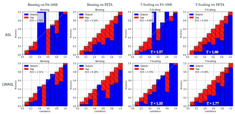
Figure 1: Reliability Diagrams for ALM and LWALM.

Reliability Diagrams

Reliability diagrams are tools to visualize model calibration [6]. A diagonal line represents the identity function, and any deviation from the diagonal represents miscalibration. These diagrams are plotted as accuracy with confidence [6]. All uncalibrated predictions $\widehat{p}_{i}$ corresponding to $I$ attributes ($i=1,2,\ldots,I$) for all samples are divided into the mutually exclusive bins $B_{1},B_{2},\ldots,B_{M},$ and the bin boundaries $0=a_{1}\leq a_{2}\leq\cdots\leq a_{M+1}=1$, where the bin $B_{m}$ is defined as the interval $(a_{m},a_{m+1}]$. Given fixed bin boundaries for the bin $B_{m}$ with interval $(a_{m},a_{m+1}]$ consisting of positive-class samples and predictions $\widehat{p}_{i}$ in the interval $(a_{m},a_{m+1}],$ their accuracy and confidence can be calculated as follows

$$Acc(B_{m})=({\sum_{p_{i}\in B_{m}}p_{i}})\,/\,|\,{\{\widehat{p}_{i}|a_{m}\leq\widehat{p}_{i}<a_{m+1}}\}|,$$ (3)

$$Conf(B_{m})=({\sum_{\widehat{p}_{i}\in B_{m}}\widehat{p}_{i}})\,/\,|\,{\{\widehat{p}_{i}|a_{m}\leq\widehat{p}_{i}<a_{m+1}}\}|,$$ (4)

where, ${p_{i}},\,i=1,2\ldots,I$ are the true labels.

Expected Calibration Error (ECE)

ECE is a scalar representation for model calibration and is approximated by first partitioning uncalibrated predictions $\widehat{p}_{i}$ and its corresponding true labels ${p_{i}}$ into $M$ bins. Then a weighted average of the bins accuracy/confidence difference is taken as follows:

$$ECE={\sum_{m=1}^{M}}\left(\frac{|a_{m}\leq\widehat{p}_{i}<a_{m+1}|}{n}\right)\left({|Acc(B_{m})-Conf(B_{m})|}\right),$$

where $n$ is the number of samples and the difference between Acc(uracy) and Conf(idence) on the right-hand side gives calibration gap. [6].

Temperature Scaling

For Temperature scaling a calibrated probability ${{q}_{i}}$ is generated based on the raw output (Logits) ${\widehat{q}_{i}}$. Then, the TS for a learned temperature $T$, is calculated as ${\widehat{q}_{i}}/T$. The optimal Temperature or the scaling factor (T) for a trained LWALM is obtained by minimizing the Weighted Binary Cross-Entropy (BCE) loss as follows:

$$\ell(p_{i},\widehat{q}_{i})={{\epsilon^{(p_{i}+(1-2p_{i})W)}p_{i}\log(\widehat{q}_{i})+(1-p_{i})\log(1-\widehat{q}_{i})}},$$

where $W$ is the initialized weight.

We represent the calibrated model using reliability diagrams, gap metric and Expected Calibration Error (ECE) with 10 bins on both datasets (PETA and PA-100K) in Figure 1. It can be observed that both ALM and LWALM experience some level of miscalibration, with ECE roughly between 2$\%$ to 12$\%$. However, ALM shows a slightly higher calibration error (2.76%, 9.20% & 4.79%, 9.29%) compared to its LW counterpart (2.51%, 8.28% & 3.79%, 8.38%) on both datasets.

8. Conclusion and Future works

In this paper, we proposed LWALMs for the PAR task, that were obtained by compressing layers of the Attribute Localization model (ALM) using a stable CPD-EPC algorithm at two stages ($\delta=0.001$ and $\delta=0.002$). LWALMs achieve high speedup with less than 2% accuracy drop for tests conducted on multiple Pedestrian datasets trained on the proposed loss function using Pedestrian Attribute Recognition (PAR) metrics. Independent evaluations using reliability diagrams on metrics such as ECE show that LWALMs well-preserve the true correctness despite changes in layer architecture and weights after compression. However, accuracy can be further improved by exploring different optimization techniques and by scaling learned parameters during training which will be a part of our future work. Moreover, we plan to explore the possibility of obtaining LWALMs by exploiting algorithms based on tensor network, such as Tensor Chain or Tensor Train decompositions.

Ashish Jha, Dimitrii Ermilov, and Konstantin Sobolev are Ph.D. candidates in Computational Data Science And Engineering at Skolkovo Institute of Science And Technology, Moscow, Russia. Contact them at {Ashish.Jha, Dmitrii.Ermilov, Konstantin.Sobolev}@skoltech.ru.

Anh Huy Phan is an associate professor at Skolkovo Institute of Science and Technology. Contact him at a.phan@skoltech.ru.

Salman Ahmadi-Asl is a research scientist at Skolkovo Institute of Science and Technology, Moscow, Russia. Contact him at S.Asl@skoltech.ru.

Naveed Ahmed is an associate professor at the University of Sharjah. Contact him at nahmed@sharjah.ac.ae.

Imran Junejo is a senior technical scientist at Advanced Technology Group, AMD, Canada. Contact him at Imran.Junejo@amd.com.

Zaher AL Aghbari (Senior Member, IEEE) is a professor at University of Sharjah. Contact him at zaher@sharjah.ac.ae.

Thar Baker(Senior Member, IEEE)(Senior Fellow, HEA) is a professor at the University of Brighton (UoB) in the UK. Contact him at t.shamsa@brighton.ac.uk.

Ahmed Mohamed Khedr is a professor at the department of Computer Science, University of Sharjah. Contact him at akhedr@sharjah.ac.ae.

Andrzej Cichocki (Fellow, IEEE) is a professor with the Skolkovo Institute of Science and Technology (Russia). Contact him at A.Cichocki@skoltech.ru.

REFERENCES

- [1] C. H. Davis. The binary search algorithm. American Documentation, 20:167–167, 1969.
- [2] Y. Deng, P. Luo, C. C. Loy, and X. Tang. Pedestrian attribute recognition at far distance. In Proceedings of the 22nd ACM international conference on Multimedia, pages 789–792, 2014.
- [3] M. Denil, B. Shakibi, L. Dinh, M. Ranzato, and N. De Freitas. Predicting parameters in deep learning. Advances in neural information processing systems, 26, 2013.
- [4] E. L. Denton, W. Zaremba, J. Bruna, Y. LeCun, and R. Fergus. Exploiting linear structure within convolutional networks for efficient evaluation. Advances in neural information processing systems, 27, 2014.
- [5] Y. Gong, L. Liu, M. Yang, and L. Bourdev. Compressing deep convolutional networks using vector quantization. arXiv preprint arXiv:1412.6115, 2014.
- [6] C. Guo, G. Pleiss, Y. Sun, and K. Q. Weinberger. On calibration of modern neural networks. In International conference on machine learning, pages 1321–1330. PMLR, 2017.
- [7] S. Han, H. Mao, and W. J. Dally. Deep compression: Compressing deep neural networks with pruning, trained quantization and huffman coding. arXiv preprint arXiv:1510.00149, 2015.
- [8] P. M. L. Hanie Sedghi, Vineet Gupta. The Singular Values of Convolutional Layers. arXiv preprint arXiv:1805.10408, 1805.10408, 2018.
- [9] F. L. Hitchcock. The expression of a tensor or a polyadic as a sum of products. Journal of Mathematics and Physics, 6(1-4):164–189, 1927.
- [10] V. Lebedev, Y. Ganin, M. Rakhuba, I. Oseledets, and V. Lempitsky. Speeding-up convolutional neural networks using fine-tuned cp-decomposition. arXiv preprint arXiv:1412.6553, 2014.
- [11] D. Li, X. Chen, and K. Huang. Multi-attribute learning for pedestrian attribute recognition in surveil- lance scenarios. In 2015 3rd IAPR Asian Conference on Pattern Recognition (ACPR), pages 111–115, 2015.
- [12] D. Li, X. Chen, and K. Huang. Multi-attribute learning for pedestrian attribute recognition in surveil- lance scenarios. In 2015 3rd IAPR Asian Conference on Pattern Recognition (ACPR), pages 111–115. IEEE, 2015.
- [13] X. Liu, H. Zhao, M. Tian, L. Sheng, J. Shao, S. Yi, J. Yan, and X. Wang. HydraPlus-Net: Attentive Deep Features for Pedestrian Analysis. pages 350–359, 10 2017.
- [14] M. Mathieu, M. Henaff, and Y. LeCun. Fast training of convolutional networks through ffts. arXiv preprint arXiv:1312.5851, 2013.
- [15] A. Novikov, D. Podoprikhin, A. Osokin, and D. P. Vetrov. Tensorizing neural networks. Advances in neural information processing systems, 28, 2015.
- [16] A.-H. Phan, P. Tichavsk‘y, and A. Cichocki. Error preserving correction: A method for CP decomposition at a target error bound. IEEE Transactions on Signal Processing, 67(5):1175–1190, 2018.
- [17] C. Tang, L. Sheng, Z. Zhang, and X. Hu. Improving Pedestrian Attribute Recognition With Weakly- Supervised Multi-Scale Attribute-Specific Localization. In Proceedings of the IEEE International Conference on Computer Vision, pages 4997–5006, 2019.
- [18] V. Vanhoucke, A. Senior, and M. Z. Mao. Improving the speed of neural networks on cpus. 2011.
- [19] H. Yang, M. Tang, W. Wen, F. Yan, D. Hu, A. Li, and Y. Chen. Learning low-rank deep neural networks via singular vector orthogonality regularization and singular value sparsification. pages 2899–2908, 06 2020