Efficient Search and Detection of Relevant Plant Parts using Semantics-Aware Active Vision

Abstract

To automate harvesting and de-leafing of tomato plants using robots, it is important to search and detect the relevant plant parts, namely tomatoes, peduncles, and petioles. This is challenging due to high levels of occlusion in tomato greenhouses. Active vision is a promising approach which helps robots to deliberately plan camera viewpoints to overcome occlusion and improve perception accuracy. However, current active-vision algorithms cannot differentiate between relevant and irrelevant plant parts, making them inefficient for targeted perception of specific plant parts. We propose a semantic active-vision strategy that uses semantic information to identify the relevant plant parts and prioritises them during view planning using an attention mechanism. We evaluated our strategy using 3D models of tomato plants with varying structural complexity, which closely represented occlusions in the real world. We used a simulated environment to gain insights into our strategy, while ensuring repeatability and statistical significance. At the end of ten viewpoints, our strategy was able to correctly detect $85.5\%$ of the plant parts, about $4$ parts more on average per plant compared to a volumetric active-vision strategy. Also, it detected $5$ and $9$ parts more compared to two predefined strategies and $11$ parts more compared to a random strategy. It also performed reliably with a median of $88.9\%$ correctly-detected objects per plant in $96$ experiments. Our strategy was also robust to uncertainty in plant and plant-part position, plant complexity, and different viewpoint sampling strategies. We believe that our work could significantly improve the speed and robustness of automated harvesting and de-leafing in tomato crop production.

I Introduction

Tomatoes are among the most consumed vegetables globally [1], with demand growing rapidly due to increasing population. However, the current rate of tomato production cannot satisfy the future demand and efforts to improve production are limited by labour shortages. The current labour force is aging, as younger generations are not interested in the physically demanding and monotonous work in the tomato industry [2]. To improve production and meet the rising demand, there is a strong need for automation, where robots can fill-in for humans and carry out the labour-intensive tasks in tomato greenhouses, such as selective harvesting and de-leafing [3].

To automate harvesting and de-leafing of tomato plants, robots must accurately detect the relevant plant parts. For harvesting, it is relevant to detect ripe tomatoes and peduncles (part that connects tomatoes to the stem). Similarly, for de-leafing, it is relevant to detect the petioles (part that connects leafs to the stem). These plant parts are shown in Figure 1. With advancements in computer vision, the detection of tomatoes, peduncles, and petioles can be achieved using cameras and artificial neural networks [4]. However, accurate and fast detection of plant parts remains challenging [5], primarily due to occlusion of the relevant plant parts by other parts, leading to incomplete or ambiguous information.

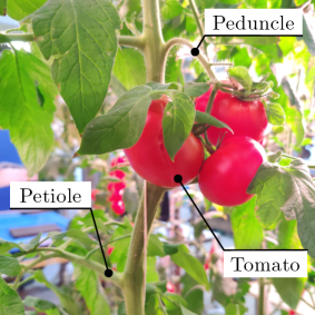
Figure 1: Accurate and efficient detection of relevant plant-parts, such as tomatoes, peduncles, and petioles, is essential for automation of harvesting and de-leafing in tomato greenhouses.

One way to overcome occlusion is to explore the plant using multiple viewpoints for detection, as acquiring multiple measurements can help fill any missing information or resolve ambiguities [6, 7]. However, the multiple viewpoints must be chosen efficiently. In current practice, passive multi-view approaches are used, in which a camera is moved in predefined patterns (e.g. zig-zag motions). These approaches often suffer from sub-optimal view selection, i.e., they are either time consuming due to too many viewpoints or fail to detect all plant parts due to too few viewpoints.

Active vision [8, 9, 10, 11] can help explore the plant faster [12, 13, 14, 15] by choosing camera viewpoints that maximise novel information about the plant. However, most active-vision algorithms are designed to explore unknown space using occupancy information, which is ideal for exploring the whole plant. The occupancy information cannot distinguish between different plant parts and hence not suitable for targeted perception of specific objects-of-interest (OOIs), such as the relevant plant parts. To address this problem, active-vision algorithms must be made aware of the OOIs. Adding semantic information about objects, such as class labels, has been shown to improve targeted perception [16] and scene understanding [17] in other applications. This has not been studied in agro-food robotics. In [13] and [14], a binary distinction between fruits and the rest of the plant was made, but the semantic information was not directly used for planning viewpoints.

In this paper, we proposed a semantic active-vision strategy that considers the class labels and confidence scores of the OOIs when planning viewpoints. We hypothesised that using such semantic information will lead to more accurate and faster perception of the relevant plant parts. Our previous work [15] demonstrated the benefit of an attention mechanism for targeted perception of plant parts, such as petioles. In this paper, we used the detected OOIs as regions of attention to guide the planner to maximise novel information about the OOIs. Unlike [15], the OOI positions were not known a priori in this work, but were estimated on-the-run. We used a simulated environment to systematically analyse the perception behaviour of our strategy and compared its performance with other planners. We hope that the insights of this work contributes to efficient robotic perception and advances automation in greenhouse crop production.

Our main contributions can be summarised as:

• We evaluated if the efficiency of search and detection of relevant plant parts can be improved by adding semantic information to active vision and enabling it to distinguish between plant parts.

• We developed an online active-vision strategy with an adaptive attention mechanism to guide the camera towards relevant plant parts and improve their perception.

• We demonstrated an attention mechanism that can simultaneously explore new plant parts and improve the quality of previously detected plant parts.

• In a simulated environment, we analysed the effect of experimental and model parameters on the performance of our strategy and tested its robustness.

II Problem description and setup

II-A Problem description

Given a tomato plant, placed within a bounded 3D space $V\subset\mathbb{R}^{3}$, the task is to explore the plant using a robot with an RGB-D camera and detect all the OOIs. The robot does not know the exact position of the plant, except that the plant is somewhere in front of it, as would be the case in an actual greenhouse. Hence, the position of the plant base $p_{\text{pb}}\in V$ contains some uncertainty. The robot starts from an initial camera viewpoint $v_{0}$ and needs to find a set of sequential viewpoints that will lead to the detection of the OOIs. Since the structure of the plant is not known a priori, the robot needs to simultaneously explore the plant to find new OOIs and improve the perception of previously detected OOIs. We formulate this task of visual search for OOIs as an online next-best-view (NBV) planning problem within the active-vision paradigm. The goal of NBV planning is to determine the next-best camera viewpoint $v_{\text{best}}$ that will help perceive novel information about the OOIs. We assume that by maximising the novel information about the OOIs per viewpoint, we can find the shortest sequence of viewpoints that can detect most of the OOIs with high accuracy. The problem is terminated when all the OOIs are detected or when a maximum number of viewing actions $a_{\text{max}}$ is reached.

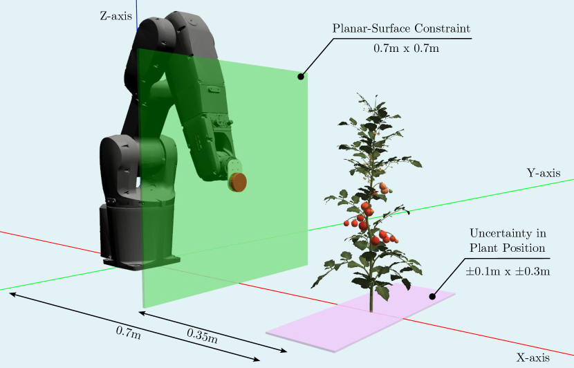
Figure 2: Schematic diagram of the experimental setup in simulation, with an ABB IRB 1200 robotic arm and Realsense L515 camera. The plant was positioned in front of the robot with uncertainty (shown in pink) to test the robustness of the viewpoint planners. The robot was allowed to choose viewpoints on a planar-surface constraint (shown in green) with $4$ DoF.

II-B Simulation setup

We used a simulated environment with Gazebo to actualise the above problem description. The simulation setup is illustrated in Figure 2. The robotic setup consisted of a $6$ degrees-of-freedom (DoF) robotic arm (ABB’s IRB 1200) with an RGB-D camera (Intel Realsense L515) attached to its end-effector. We used eight 3D mesh models of tomato plants of varying growth stages and structural complexity, which the robot explored to detect the OOIs. A tomato plant was placed in front of the robot at $p_{\text{pb}}=(0.7\pm 0.1\text{m},0.0\pm 0.3\text{m},0.8\text{m})$. Uncertainty was introduced in the plant-base position by uniformly sampling the x and y positions in the range $0.7\pm 0.1$m and $0.0\pm 0.3$m respectively.

A planar-surface constraint was used for view planning, i.e., the robot could choose viewpoints only within the bounds of the plane. The planar surface was of size $0.7\times 0.7$ m², with its center at a distance of $0.35$m from the plant and at a height of $0.8$m. In addition to positioning the camera on the planar surface, the viewpoints could also make a pan and tilt of $0\pm 15^{\circ}$, which were uniformly sampled. Hence, the viewpoints had $4$ DoF. All the viewpoint planners started from the same initial viewpoint $v_{0}$ with position (xyz) $(0.35,0.22,0.90)^{T}$ and orientation (xyzw) $(0.00,0.00,-0.26,0.97)^{T}$. The robot was allowed to choose a maximum of $a_{\text{max}}=10$ consecutive viewing actions to explore the plant and identify as many OOIs as possible.

III Semantic next-best-view planning

To address the problem described above, we proposed a Semantic NBV planning algorithm. The main loop of the planner is illustrated in Figure 3. The algorithm consisted of three major modules – (i) a sensing module to detect the OOIs, (ii) a 3D representation module to merge information about the OOIs across multiple viewpoints, and (iii) a view-planning module to determine the next-best camera viewpoint.

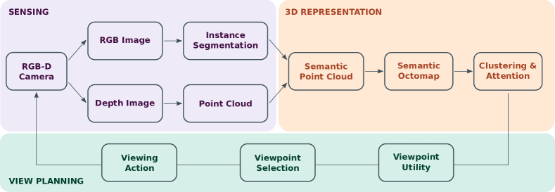
Figure 3: The main pipeline of the Semantic NBV planning algorithm consists of three major modules – (i) a sensing module to detect OOIs (Sec. III-A), (ii) a 3D representation module to analyse and track the OOIs over multiple viewpoints (Sec. III-B to III-E), and (iii) a view-planning module to determine the next-best camera viewpoint (Sec. III-F, III-G).

III-A Sensing

The first step of the algorithm was to accurately detect the OOIs. For this, we used a convolutional neural network called Mask R-CNN [18]. We fine-tuned the network to detect tomatoes, peduncles, and petioles using a custom dataset of $90$ RGB images, of dimension $960\times 540$ pixels, collected from the simulated environment. The dataset was split into $72$ images for training and $18$ images for validation. The network took an RGB image as input and generated a segmented image with masks that separated the OOIs from the background (Fig. 4(a)).

III-B Semantic Point Cloud

The segmented image was combined with the corresponding depth image to generate a semantic point cloud (Fig. 4(b)). Each point $i$ in the point cloud contained spatial position $p(i)\in V$ of the OOIs in Cartesian space and also the class label $c(i)$ and confidence score $P_{s}(i)$ about what object the point belonged to. The class label and confidence score were defined as,

$$c(i) \in\{0=\text{peduncle},1=\text{petiole},2=\text{tomato}\},$$ (1)

$$P_{s}(i) \in[0,1].$$ (2)

The confidence score $P_{s}(i)$ was interpreted as the probability of the point $i$ belonging to the detected class label $c_{i}$. Hence, $P_{s}(i)=0$ meant that the point certainly did not belong to $c_{i}$, whereas $P_{s}(i)=1$ meant that the point certainly belonged to $c_{i}$. The values inbetween implied uncertainty regarding the class label, with maximum uncertainty at $P_{s}(i)=0.5$. If a point did not contain any semantic information, a default value of $c_{i}=-1$ and $P_{s}(i)=0.5$ were assigned, which meant that the point belonged to the background and had maximum uncertainty regarding its class label.

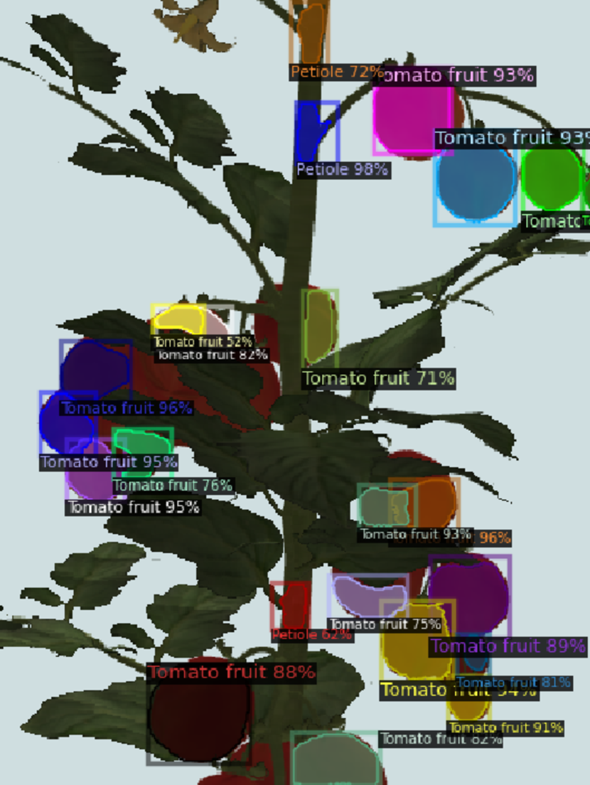
(a)

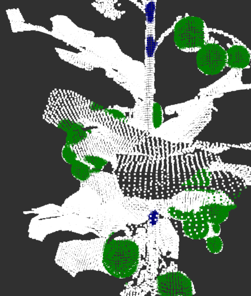
(b)

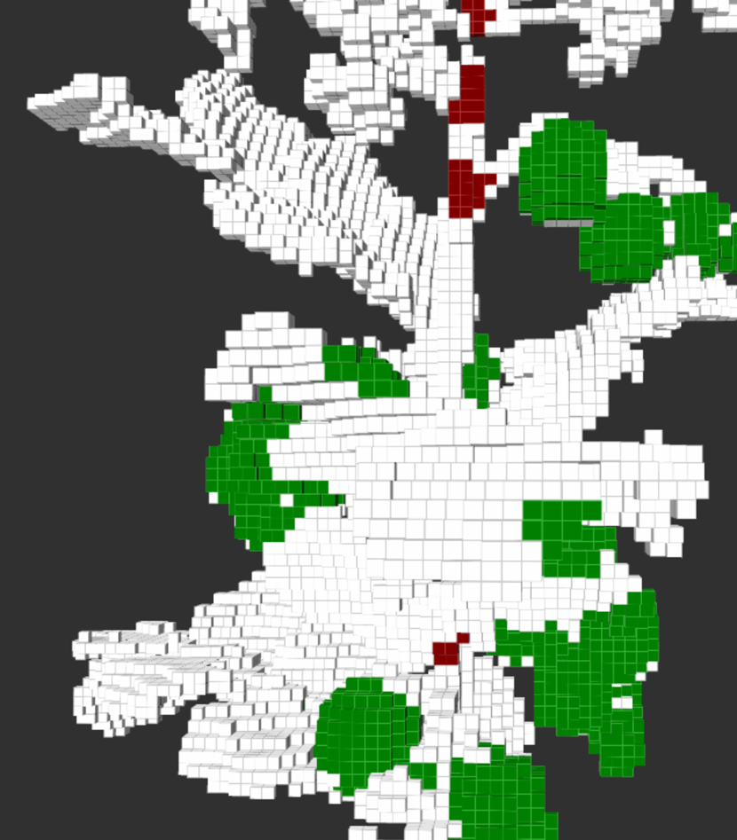
(c)

Figure 4: Generating the semantic OctoMap had the following steps: (a) The objects-of-interest (OOIs), were detected using Mask R-CNN to form a segmented image (Sec. III-A). (b) The segmented image was combined with the corresponding depth image to produce a semantic point cloud (Sec. III-B). (c) The semantic point cloud was then inserted into the OctoMap, where each voxel stores the class label and confidence score, along with the occupancy probability (Sec. III-C). Also, a clustering operation was performed on the semantic OctoMap to identify the individual OOIs at an object level in 3D space (Sec. III-D).

$\xrightarrow{}$ $\xrightarrow{}$

III-C Semantic OctoMap

The semantic point cloud captured the spatial and semantic information of the plant only in the current viewpoint. To keep track of the detected OOIs across multiple viewpoints, we needed a 3D representation of the plant which could be updated over time. So, we represented the observed plant and its surrounding scene as a probabilistic occupancy map called an OctoMap [19]. The OctoMap divided the 3D space into grid cells called voxels, which were efficiently stored as hierarchical nodes in an Octree. We used a resolution of $0.003$m for a single voxel. Each voxel was marked as empty or occupied based on whether the voxel was observed by the camera. Voxels with an occupancy probability of zero ($P_{o}=0$) were considered empty and those with occupancy probability of one ($P_{o}=1$) were considered occupied. A value between $0$ and $1$ implied uncertainty regarding the occupancy, with a maximum uncertainty at $P_{o}=0.5$. The regions that were not observed by the camera yet did not contain any occupancy information and were considered unknown with maximum uncertainty ($P_{o}=0.5$). Such information about the occupancy probabilities of the voxels is commonly referred to as volumetric information. The volumetric information is useful in identifying the uncertain and unexplored regions of the plant, and can help guide an NBV planner towards them. However, it cannot distinguish between different plant parts and hence not suitable for targeted perception of the OOIs.

To be able to explore the OOIs, we extended the OctoMap to include semantic information in addition to the volumetric information (Fig. 4(c)), similar to [20]. The semantic information consisted of a class label and a confidence score that was obtained from the semantic point cloud in the previous step (Sec. III-B). The class labels identified the OOIs and distinguished them from the rest of the plant, while the confidence scores indicated how certain we were about the OOI identities. Hence, the semantic OctoMap can help guide an NBV planner to search for OOIs and further explore them until a degree of certainty is achieved.

When new camera observations were made, the semantic information was updated in the semantic OctoMap. The semantic information, i.e. the class labels $c(i)$ and confidence scores $P_{s}(i)$ obtained from Mask R-CNN (Sec. III-A), was inserted into corresponding voxels in the OctoMap. This operation was only performed for points with a valid class label. If the voxel had no prior semantic information, the values were directly assigned to it. Otherwise, the semantic information was updated using the method of max-fusion from [20]. The new class label and confidence score from the semantic point cloud were merged with the previous values in the voxel as follows: (i) if the new class label was the same as the previous, then the class label remained unchanged and the confidence score was computed as the average of the new and previous scores; or (ii) if the new class label was different from the previous, the semantic label with the higher confidence score was chosen and that confidence score was reduced by $10\%$ as a penalty for label mismatch. The max-fusion method was used as it was simple, fast and memory-efficient as it only stores one class label and confidence score per voxel. The pseudo code for the max-fusion method is shown in Algorithm 1. For a voxel $x$, the class label and confidence score contained in the voxel were denoted as $c(x)$ and $P_{s}(x)$ respectively.

Algorithm 1 Max fusion

$\text{sem}_{1},\text{sem}_{2}$ $\triangleright$ Previous and new semantics

$\text{sem}_{f}$ $\triangleright$ Updated semantics

$c,P_{s}$ $\triangleright$ Class label and confidence score

function Max Fusion($\text{sem}_{1},\text{sem}_{2}$)

     if $\text{sem}_{1}.c==\text{sem}_{2}.c$ then

         $\text{sem}_{f}.c\leftarrow\text{sem}_{2}.c$

         $\text{sem}_{f}.P_{s}\leftarrow(\text{sem}_{1}.P_{s}+\text{sem}_{2}.P_{s})/2$

     else

         $\text{sem}_{f}.c\leftarrow\arg\max_{c}(\text{sem}_{1}.P_{s},\text{sem}_{2}.P_{s})$

         $\text{sem}_{f}.P_{s}\leftarrow 0.9\times\max(\text{sem}_{1}.P_{s},\text{sem}_{2}.P_{s})$      return $\text{sem}_{f}$

III-D Clustering

The semantic OctoMap represented the OOIs in a discretised form at the voxel-level. However, an object-level representation was required to count and locate the OOIs in 3D space. We achieved this by clustering the voxels that belong to the same object. We used an algorithm called Ordering Points To Identify the Clustering Structure (OPTICS) [21]. Each cluster was identified by three criteria – (i) all voxels in the cluster must belong to an OOI, (ii) the total number of voxels in a cluster must be at least $20$, and (iii) the maximum distance between any two voxels within the cluster is $0.03$m, which was roughly the size of the OOIs in simulation. With this clustering step, we got an object-level representation of the OOIs. The number of detected OOIs was given by the number of clusters, and the positions of the OOIs $p_{\text{ooi}}\in V$ were given by the center of the clusters. The clustering was repeated at every iteration of the Semantic NBV planning pipeline. Hence, as the semantic OctoMap got updated over multiple viewpoints (Sec. III-C), the OOIs were also updated.

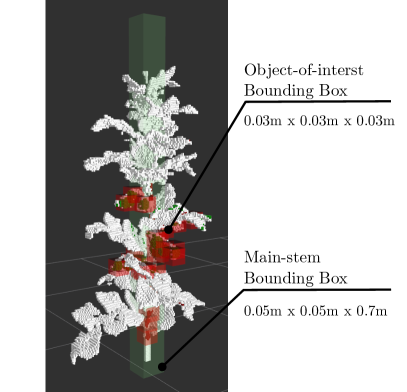
Figure 5: An attention mechanism was used to guide the Semantic NBV planner. A region-of-interest was defined along the estimated position of the main stem (green bounding box) to guide the planner to explore new OOIs. Multiple regions-of-interest were defined around the detected OOIs (red bounding boxes) to guide the planner to perceive them more accurately.

III-E Attention mechanism

An object-level representation of OOIs allows the NBV planner to attend to regions where the OOIs are located and improve their accuracy. So, similar to our previous work [15], we used an attention mechanism to guide the NBV planner to explore and perceive the OOIs. We marked the attention regions by defining bounding boxes around the estimated position of the main stem and the detected positions of the OOIs, as shown in Figure 5. The main-stem bounding box guided the planner to explore and identify new OOIs, while the OOI bounding boxes guided the planner to perceive the detected OOIs more accurately. While [13] had to define two separate strategies to obtain these behaviours, we were able to obtain them with a single strategy. The bounding boxes were axis-aligned and were defined using six parameters – the center of the box and the dimension of the sides. The regions of attention for the main stem and the OOIs were defined as:

III-E1 Attention on the main stem

To define an attention region along the main stem, the position of the main-stem center $p_{\text{ms}}\in V$ had to be estimated. We assumed that $p_{\text{ms}}$ was fixed at a height of $1.15$m along the z-axis. So, only the position along the $x$ and $y$ axes were estimated. The position of the main stem was not detected directly, but estimated based on the amount of information perceived about the plant. (i) When there was no information about the plant at all, the main-stem position was not defined. (ii) Once the plant was in view, the main-stem position was estimated as the center of the visible region of the plant, which guided the NBV planner to explore the plant further. (iii) Once some of the OOI clusters were detected, the main-stem position was estimated as the center of the OOI clusters instead. Since the OOIs are attached to the main stem, we assumed the main stem to roughly lie in their center. The estimated position of the main stem was incorrect at the beginning, but it gradually improved as more viewpoints were taken and more information about the plant became available.

The main-stem bounding box was defined only when the main-stem position could be estimated. Until then, the NBV planner planned viewpoints without an attention mechanism. The estimated main-stem position $p_{\text{ms}}$ was used to define the center of the main-stem bounding box. The size of the bounding box was predefined with a width and breadth of $0.05$m and height of $0.7$m (Fig. 5). As the estimation of the main-stem position improved with multiple viewpoints, the bounding box was adapted iteratively.

III-E2 Attention on the OOIs

An OOI bounding box was defined only when an OOI cluster was detected (Sec. III-D). The position of the OOI $p_{\text{ooi}}$ was used to define the center of the OOI bounding box. The size of the bounding box was predefined as a cube with size $0.03$m (Fig. 5). These bounding boxes automatically adapted to any changes in the OOI clusters, such as a shift in the position or being completely removed if the cluster was not detected anymore.

III-F Viewpoint Utility

The selection of the next-best viewpoint was guided by a metric called expected information gain, which estimated the amount of novel information that could be obtained when a camera was moved to a given viewpoint. For the Semantic NBV planner, we defined the information gain using the semantic information in the OctoMap.

III-F1 Expected semantic information gain

The semantic information gain is a measure of how much novel semantic information can be gained by exploring a 3D volume. The semantic information $I_{\text{sem}}$ expected to be gained by observing a voxel $x$ was defined as its entropy,

$$I_{\text{sem}}(x)=-P_{s}(x)\log_{2}(P_{s}(x))-(1-P_{s}(x))\log_{2}(1-P_{s}(x)),$$ (3)

where $P_{s}(x)$ is the confidence score that the voxel $x$ belonged to a certain object. The confidence score was obtained from the semantic OctoMap as discussed in Section III-C. The information gain has a range between $0$ and $1$. Intuitively, it is high for voxels with high uncertainty (i.e. $P_{s}(x)$ close to $0.5$) and low for voxels with low uncertainty (i.e. $P_{s}(x)$ close to $0$ or $1$). Hence, it is a measure of uncertainty.

To guide the Semantic NBV planner to search for OOIs, we designed it to prioritise viewpoints that maximised the expected semantic information gain. The expected semantic information gain $G_{\text{sem}}(v)$ for a viewpoint $v$ was computed as the sum of the semantic information of all voxels that were expected to be visible from $v$, that is,

$$G_{\text{sem}}(v)=\sum_{x\in(\mathcal{X}_{v}\cap\mathcal{B})}I_{\text{sem}}(x),$$ (4)

where $\mathcal{X}_{v}$ was the set of all voxels that were expected to be visible from viewpoint $v$ and $\mathcal{B}$ was the set of all voxels that were within the attention regions (defined in Sec. III-E). $\mathcal{X}_{v}$ was determined by the process of ray-tracing, in which a set of rays were cast from viewpoint $v$ evenly across the camera’s view frustum. Each ray traversed until it hit an occupied voxel or reached a maximum distance. All voxels that the rays intersected, were expected to be visible if the camera was moved to viewpoint $v$ and hence were added to the set $\mathcal{X}_{v}$.

The Semantic NBV planner used only the semantic information and discarded the volumetric information. Such a formulation however did not limit the planner from understanding occupied and unoccupied regions of space, since the semantic information inherently contains occupancy information to some extent. For example, any voxel that contains a semantic class label is by definition occupied. However, the Semantic NBV planner gave no importance to how certain we were about the occupancy and focused primarily on how certain we were about the semantic labels.

III-F2 Total Utility

In addition to the expected semantic information gain, the distance from the current viewpoint was also considered when selecting the next viewpoint since there was a time cost for executing the motion. We approximated the time cost as the Euclidean distance between the current viewpoint and the next potential viewpoint. So, the final view utility $U$ was the expected semantic information gain $G_{\text{sem}}(v)$ scaled by the Euclidean distance cost $d$,

$$U_{\text{sem}}=G_{\text{sem}}(v)\times e^{-d},$$ (5)

where the exponential to the negative distance cost prioritized the viewpoints that were very close to the current viewpoint.

Now, the objective of NBV planner was to find a viewpoint that maximised the viewpoint utility, which would lead to efficient exploration and detection of the OOIs.

III-G Viewpoint selection

To determine the next-best viewpoint, we sampled a set of $27$ candidates $\mathcal{V}$ at each step within the planar-surface constraint, defined in Section II-B. These candidates were potential viewpoints where the camera could be moved next. For each candidate, the view utility was computed using Equation 5, and the viewpoint with the maximum utility was chosen as the next-best viewpoint,

$$v_{\text{best}}=\underset{v\in\mathcal{V}}{\arg\max}\;U_{\text{sem}}.$$ (6)

Sampling the candidates is an important step for view selection. If all the candidates were poor choices, we would end up with an inefficient sequence of viewpoints despite maximising the information gain at each step. Hence, we used a pseudo-random sampling strategy, similar to our previous work [15], which evenly distributed the candidates across the planar surface. This strategy tried to ensure that there were at least a few candidates, choosing whom, would lead to efficient exploration of OOIs. Although, this was not guaranteed.

IV Existing methods for comparison

We compared the performance of the Semantic NBV planner with a Volumetric NBV planner [15], two predefined planners and a random planner as baseline.

IV-A Volumetric NBV planner

The Volumetric NBV planner is the most common approach in NBV planning, which uses the expected gain in volumetric information to determine the next-best viewpoint. It tends to explore all uncertain regions of the plant, which is suitable for whole-plant perception. Similar to semantic information gain, the volumetric information gain is a measure of how much novel volumetric information can be gained by exploring a 3D volume. The volumetric information $I_{\text{vol}}$ expected to be gained by observing a single voxel $x$ was defined as,

$$I_{\text{vol}}(x)=-P_{o}(x)\log_{2}(P_{o}(x))-(1-P_{o}(x))\log_{2}(1-P_{o}(x)),$$ (7)

where $P_{o}(x)$ is the probability of voxel $x$ being occupied. The expected volumetric information gain $G_{\text{vol}}(v)$ for a viewpoint $v$ was then computed as the sum of the volumetric information of all voxels that were expected to be visible from $v$, that is,

$$G_{\text{vol}}(v)=\sum_{x\in(\mathcal{X}_{v}\cap\mathcal{B})}I_{\text{vol}}(x),$$ (8)

where $\mathcal{X}_{v}$ was the set of all voxels that were expected to be visible from viewpoint $v$ and $\mathcal{B}$ was the set of all voxels that were within the attention regions. The Volumetric NBV planner was implemented by using $G_{\text{vol}}(v)$ for computing the view utility and view selection. Hence, the Eqs. 5 and 6 were modified as follows,

$$U_{\text{vol}} =G_{\text{vol}}(v)\times e^{-d},$$ (9)

$$v_{\text{best}} =\underset{v\in\mathcal{V}}{\arg\max}\;U_{\text{vol}}.$$ (10)

We also provided an adaptive attention mechanism for the Volumetric NBV planner to focus on the main stem (similar to Sec. III-E1). The Volumetric NBV planner was similar to the Semantic NBV planner, expect that it used $G_{\text{vol}}(v)$ instead of $G_{\text{sem}}(v)$ and did not use OOI bounding boxes.

IV-B Pre-defiend planners

We used two predefined planners with a zig-zag pattern, which is a common practice in greenhouses to detect the OOIs. Since there was a large uncertainty in plant position along the y-axis, we could not design a single predefined planner that could perceive the plant well across the whole uncertainty range ($y=\pm 0.3$m). So, we used two planners with different ranges of motion. One planner had a narrow range making an angle of $18^{\circ}$ to the center of the plant and the other had a wider range making an angle of $54^{\circ}$ (Fig. 6). The predefined planners scanned the plants from the bottom to top.

IV-C Random planner

We used a random planner that chose one viewpoint at random from the set of $27$ candidate viewpoints $\mathcal{V}$ that were sampled at each step (Sec. III-G). This planner was used a baseline to confirm that the Semantic NBV planner was more efficient than choosing a viewpoint at random.

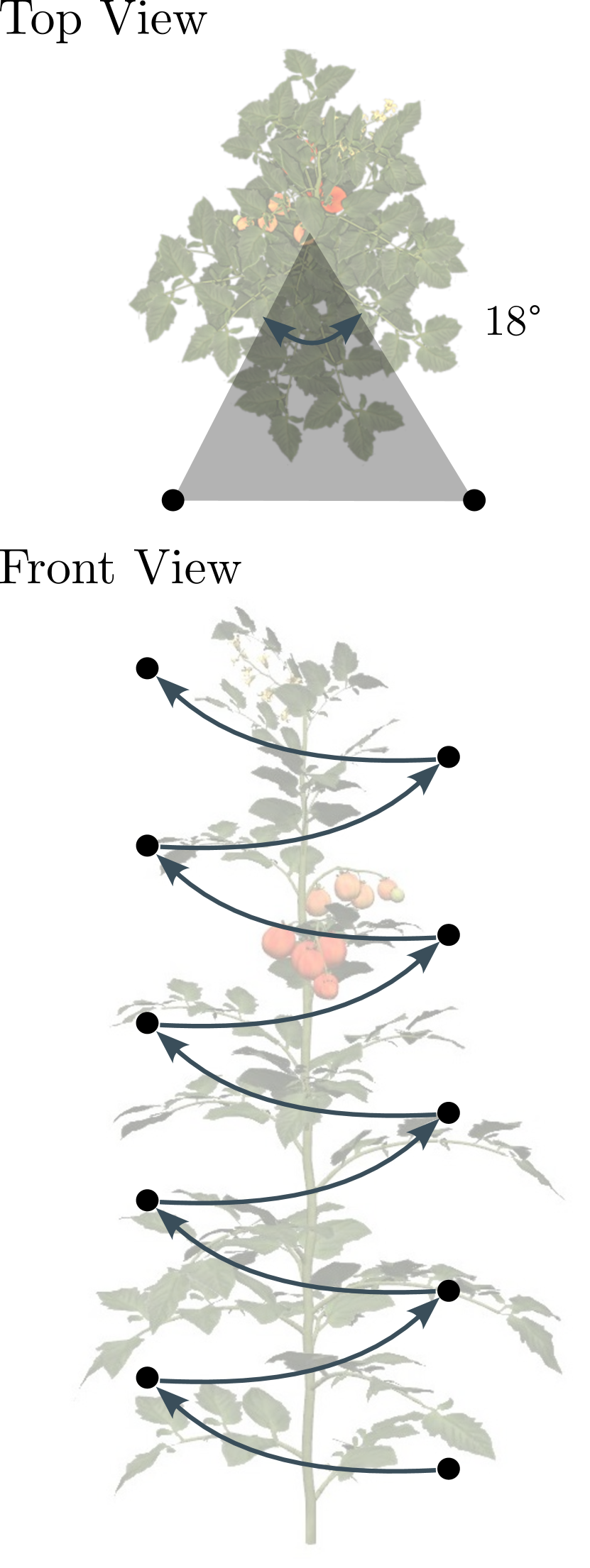
(a)

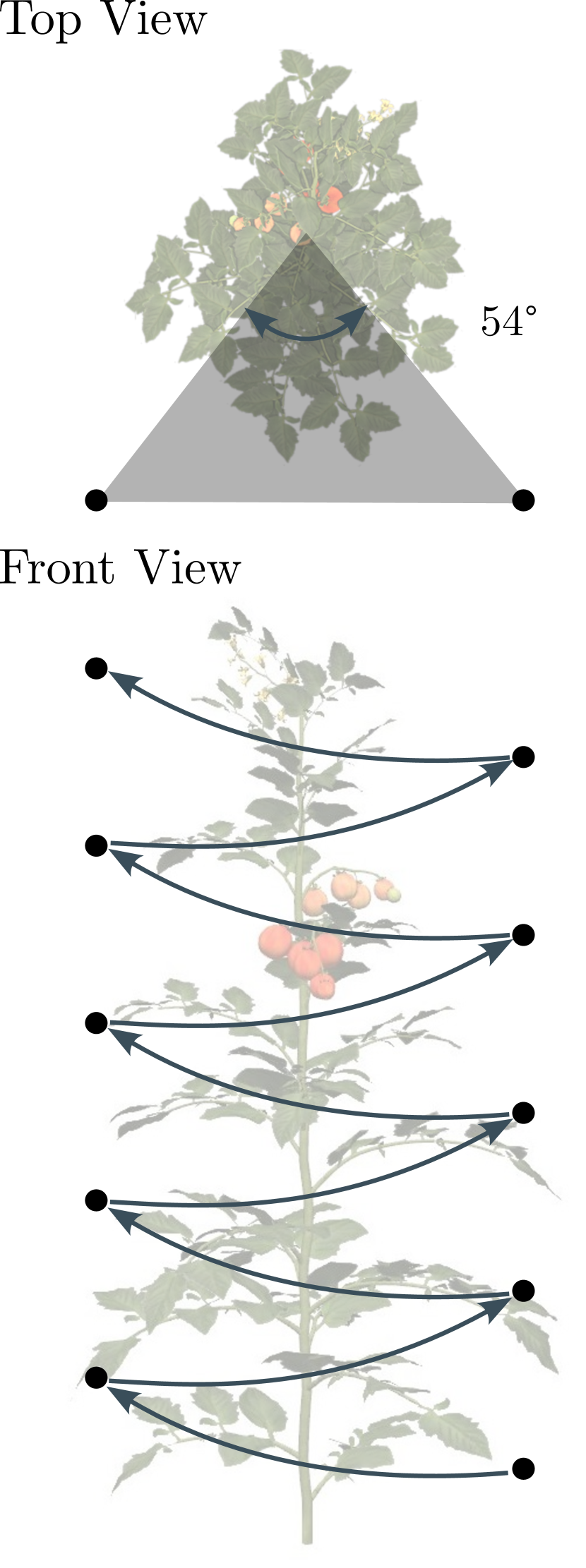
(b)

Figure 6: The performance of the Semantic NBV planner was compared with a Volumetric NBV planner, two predefined planners and a random planner. The predefined planners had ten viewpoints and differed in their range of motion: (a) Predefined Narrow planner and (b) Predefined Wide planner.

V Experiments

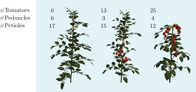
(a)

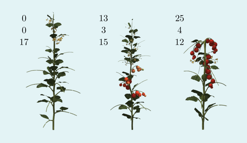
(b)

Figure 7: Eight mesh models of tomato plants were used for the experiments. The plants varied in terms of growth stage, number of OOIs, height and complexity. Some examples of (a) the original plant models and (b) the same plant models with around $50$-$60\%$ leaflets removed are shown.

We experimented with eight tomato plants, using $12$ different rotations along the z-axis at intervals of $30^{\circ}$ each, leading to a total of $96$ experiments. Figure 7 shows some examples of the plant models used.

V-A Main experiment

As our main experiment, we studied how efficiently could the Semantic NBV planner detect the OOIs compared to the Volumetric NBV, Predefined Wide, Predefined Narrow, and Random planners. The experimental setup (Sec. II-B) contained uncertainty in plant and OOI positions, high level of occlusions from plant parts, and a planar-surface constraint for sampling the candidate viewpoints. The evaluation criteria for the comparison is discussed in Section V-C.

V-B Analysis of experimental and model parameters

We also analysed the effect of the following experimental and model parameters on the planner performance:

V-B1 Impact of removing uncertainty in plant position

In practice, the exact position of the tomato plants will not be known. Hence, the Semantic NBV planner should be able to handle such uncertainty. In the main experiments, the plant positions had an uncertainty of $\pm 0.1$m in the x-axis and $\pm 0.3$m in the y-axis. We analysed the impact of this uncertainty by comparing the main experiments to a case where the exact plant positions were assumed to be known.

V-B2 Impact of removing uncertainty in OOI positions

The Semantic NBV planner has to deal with uncertainty in the OOI positions too, which could be caused due to errors in detection. The Semantic NBV planner should still be able to estimate the OOI positions accurately and define appropriate bounding boxes for attention. We analysed the impact of OOI-position uncertainty by comparing the main experiments to a case where the exact OOI-positions were known. The Volumetric NBV planner did not use attention on OOIs and hence its performance was unaffected by this parameter.

V-B3 Impact of removing attention

Our proposed attention mechanism is crucial in improving the efficiency of OOI detection. Without an attention mechanism, the planner will consider semantic information from all voxels expected to be visible from a viewpoint. Hence, it might prioritise every part of the plant instead of the OOIs alone, which could make it inefficient. We tested this hypothesis by comparing the main experiments to a case where the the main-stem bounding boxes and the OOI bounding boxes were completely removed.

V-B4 Impact of reducing plant complexity

The primary objective of the Semantic NBV planner is to detect the OOIs despite high complexity in the plant structure, where the OOIs are heavily occluded from the camera’s view. We analysed the impact of occlusion by comparing the main experiment to a case where the plant complexity was reduced by removing around $50$-$60\%$ of the leaflets, as shown in Figure 7(b).

V-B5 Sensitivity to sampling constraint

The planar-surface constraint (Sec. II-B) defined a region in which the planners could sample candidate viewpoints. We analysed the sensitivity of the planners to different sampling constraints to ensure that our results would still hold under different sampling strategies. We compared the planar-surface constraint ($4$ DoF), used in the main experiments, with a cylindrical-sector constraint ($2$ DoF), as used in [15]. Under the cylindrical-sector constraint, a viewpoint could be positioned anywhere on the cylinder surface but was always oriented towards the center of the cylinder. The cylinder had a height of $0.7$m, radius of $0.4$m and a sector angle of $90^{\circ}$.

V-C Evaluation

We evaluated the performance of the planners by calculating the percentage of OOIs that were correctly detected out of all the OOIs in each plant. We call this metric the percentage of correctly-detected objects (PCO),

$$\text{PCO}=\frac{\text{Correctly detected objects}}{\text{Total number of objects}}\times 100.$$ (11)

An object was considered correctly detected only when at least $50\%$ of the object was accurately reconstructed by the planner. This was quantified using the metric of F1-score, similar to [15]. The F1-score compares the ground-truth and reconstructed OOIs and estimates both the correctness and completeness of the reconstruction. It takes a value between $0$ and $1$, where a value of $1$ implies a complete and correct reconstruction.

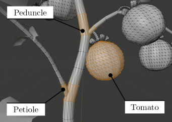
Figure 8: The ground truth for evaluation was obtained by processing the original 3D mesh of tomato plants in Blender. The ground-truth positions of the objects-of-interest (OOIs) were estimated by averaging the positions of vertices that belonged to the object. Examples of a tomato, petiole, and peduncle with their vertices highlighted (in orange) is shown.

We followed a series of steps to enable the computation of the F1-score for all the OOIs. First, the original 3D mesh of the tomato plants were converted to a point cloud and down-sampled to the same resolution as the semantic OctoMap (i.e. $0.003$m) using voxel-grid filtering. The semantic OctoMap was also converted to a point cloud, to make it comparable to the ground-truth. Only the occupied voxels were converted, i.e. voxels with $P_{o}(x)>0.5$. Second, the true position of the OOIs were obtained manually by processing the 3D mesh of the plants in Blender. For each object, the true position was calculated by averaging the positions of mesh vertices that belonged to the object, as shown in Figure 8. Finally, from both the ground-truth and reconstructed point clouds, the points belonging to each OOI was extracted by using a bounding-box of size $0.03$m and placing it at the true position of the OOI. The points within the bounding box were considered to belong to the OOI. These steps gave us the ground-truth and reconstructed point clouds for each OOI, which were then used to compute the F1-scores.

For the F1-score, we used a distance threshold equal to the voxel resolution, that is $0.003$m, which means that a point from the reconstructed OOI was considered accurate only when it was within a distance of $0.003$m from a point in the ground truth. The F1-score was computed as,

$$F_{1}=\frac{2\cdot\text{TP}}{2\cdot\text{TP}+\text{FN}+\text{FP}},$$ (12)

where TP (True Positive) refers to points in the ground truth that were accurately reconstructed, FN (False Negative) refers to points in the ground truth that were not reconstructed, and FP (False Positive) refers to points that were reconstructed but do not belong to the OOIs, that is, the reconstructed points with no corresponding ground-truth points. Once the F1-scores were computed, an object was considered correctly detected when its F1-score was greater than $0.5$, that is, at least $50\%$ of the object was reconstructed accurately.

VI Results

VI-A Main results

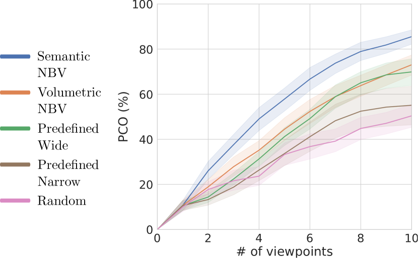
(a)

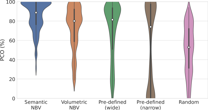
(b)

Figure 9: Performance of the planners on the detection of all objects-of-interest (OOIs) when a tomato plant was placed $0.7$m in front of the robot with an uncertainty of $\pm 0.1$m in the x-axis and $\pm 0.3$m in the y-axis. The percentage of correctly-detected objects (PCO) was determined for each viewing action. A detection was considered correct when at least 50$\%$ of the object was perceived (F1-score $>=0.5$). (a) The mean PCO of the planners at each viewing action over 96 experiments. The error bands show the $95\%$ confidence interval of the mean over all experiments. (b) The distribution density of PCO for the planners at the end of ten viewing actions over 96 experiments. The median PCO is shown by the white dot in the plot.

Figure 9(a) shows the performance of all planners on the detection of OOIs when the plants where roughly positioned in front of the robot. We observe that the Semantic NBV planner significantly outperformed the other planners in terms of PCO at each viewing action. At the end of ten viewing actions, the Semantic NBV planner was able to efficiently search and detect $85.52\%$ of the OOIs on average over 96 experiments, despite occlusions and uncertainty in plant positions. It outperformed the Volumetric NBV planner by $12.47\%$ ($\approx 4$ objects), the Predefined Wide planner by $15.64\%$ ($\approx 5$ objects), the Predefined Narrow planner by $30.43\%$ ($\approx 9$ objects), and the Random planner by $35.11\%$ ($\approx 11$ objects).

For targeted perception of plant parts, these results clearly show that viewing only the unexplored regions of the plant, as the Volumetric NBV planner, is not efficient enough. It does not perform any better than a well-designed predefined strategy, such as the Predefined Wide planner. However, by adding knowledge of semantics, the performance improved significantly since the planner was now able to distinguish between the relevant and irrelevant plant parts.

The distribution density of the PCO at the end of ten viewing actions over all 96 experiments, shown in Figure 9(b), offers further insights on the performance of the planners. We observe that the Semantic NBV planner’s performance was highly reliable as the PCO density was concentrated in the higher end with a median PCO of $88.85\%$, i.e. half the experiments had a PCO greater than this. The Volumetric NBV and Predefined Wide planners had a median PCO of $80.14\%$ and $81.48\%$ respectively, with the Volumetric NBV planner performing slightly more reliably. The Predefined Narrow and Random planners were most unreliable as their PCO densities were spread over the entire range of PCO and their median PCOs were much lower at $74.07\%$ and $52.94\%$ respectively.

VI-B Analysis of experimental and model parameters

For brevity, we only compared the three best performing planners from the main experiment, namely Semantic NBV, Volumetric NBV and Predefined Wide planners.

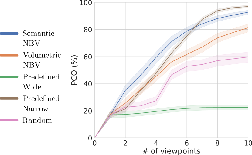
(a)

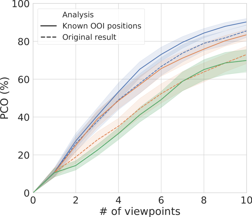
(b)

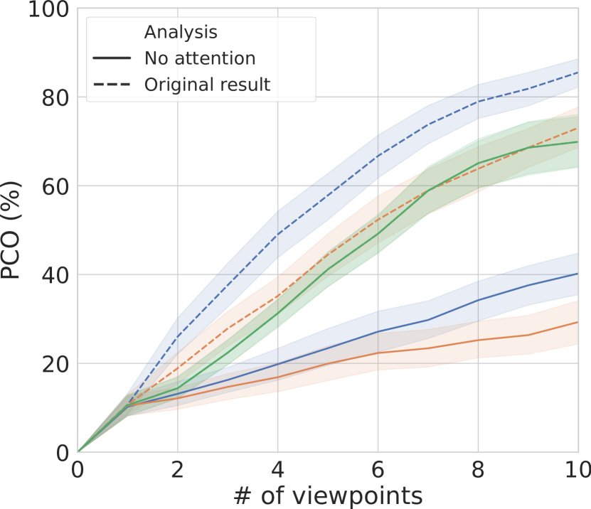
(c)

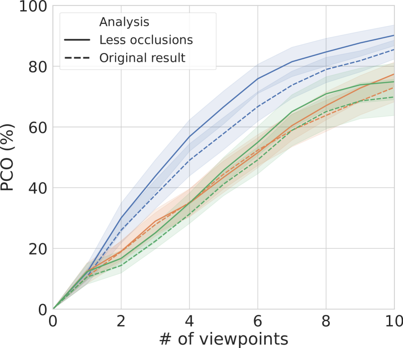
(d)

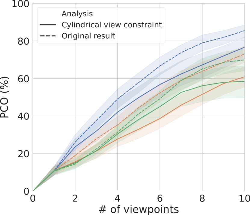
(e)

Figure 10: Analysis of the performance of the planners based on various experimental and model parameters. The plots show the impact of (a) removing uncertainty in plant position, (b) removing uncertainty in OOI position, (c) removing attention, (d) reducing plant complexity or occlusion, and (e) changing the sampling constraint. The solid lines show the updated results based on the modified parameter and the dotted lines show the original results. The error bands show the $95\%$ confidence interval of the mean over all 96 experiments. Please note: The solid and dotted lines of the Predefined Wide planner overlap each other in plots (b) and (c) since the performance of the planner was not influenced by these parameters.

VI-B1 Impact of removing uncertainty in plant position

Figure 10(a) shows the performance of the planners when the plants were placed in a fixed and known position in front of the robot. Compared to the original experiment with uncertainty in plant position (Fig. 9(a)), the Semantic NBV planner detected $7.22\%$ more OOIs in this case, since it did not have to search for the plant before detecting the OOIs. The Predefined Narrow planner performed the best by detecting $96.96\%$ of the OOIs. This indicates that the predefined planners in practice can be effective when the positions of the plants are known accurately. However, they are extremely sensitive to uncertainty in plant position and their performance can be unreliable, as seen from Figure 9(b). The Semantic and Volumetric NBV planners, on the other hand, are able to handle the uncertainty better by using the adaptive attention mechanism.

VI-B2 Impact of removing uncertainty in OOI positions

Figure 10(b) shows the performance of the planners when the true OOI positions were known, i.e., all the OOI bounding boxes were provided at the beginning of the experiments. The Semantic NBV planner showed a small improvement and could detect $4.73\%$ more OOIs compared to the original experiment. This implies that the Semantic NBV planner in the original experiment was able to explore and detect the OOIs quite reliably. Hence, its performance was close to the ideal case. On the other hand, the Volumetric NBV planner showed a larger improvement and could detect $10.42\%$ more OOIs, indicating that it could not detect the OOIs reliably in the original experiment. The poor performance of the Volumetric NBV planner was likely due to the lack of an attention mechanism to focus on the OOIs. The performance of the Predefined Wide planner was independent of the OOI positions.

VI-B3 Impact of removing attention

Figure 10(c) shows the performance of the planners in the absence of an attention mechanism. The impact of removing attention was drastic on the Semantic and Volumetric NBV planners. Their performance dropped by $45.28\%$ and $43.74\%$ respectively and they were unable to detect even half the OOIs at the end of ten viewpoints. The drop in performance was because the planners had less guidance to perceive the relevant plant parts and spent time exploring irrelevant regions. This shows the significance of an attention mechanism in making NBV planning more efficient when performing a targeted search. Interestingly, the Semantic NBV planner outperforms the Volumetric NBV planner in this case too. This shows that the addition of semantic information, by itself, is helpful in guiding the planner to detect OOIs. When combined with an attention mechanism, the performance is further enhanced.

VI-B4 Impact of reducing plant complexity

Figure 10(d) shows that the performance of all the planners improved when the plant complexity was reduced. The Semantic NBV planner could detect $4.6\%$ more OOIs, while the Volumetric NBV planner could detect $4.4\%$ more, and the Predefined Wide planner could detect $5.03\%$ more. By removing the leaflets, the OOIs were less occluded and easier to detect from many viewpoints. The fact that only a small improvement in performance was observed indicates that all the three planners were able to handle the plant complexity and occlusions in the original experiment well. The overall results were still consistent with the original results, with the Semantic NBV planner outperforming the others by a significant margin.

VI-B5 Sensitivity to sampling constraint

Figure 10(e) shows the performance of the planners when a cylindrical-sector constraint was used for view sampling (Sec. V-B5) instead of a planar-surface constraint. All the planners performed poorer in this case. The Semantic NBV planner detected $8.88\%$ less OOIs, while the Volumetric NBV planner detected $12.15\%$ less and the Predefined Wide planner detected $11.42\%$ less. Under the cylindrical-sector constraint, the viewpoints were forced to look towards the center of the cylinder, which reduced the DoF from four to two. This potentially reduced the chances of finding good viewpoints and hence led to a drop in performance for all planners. The overall results were still consistent with the original results, with the Semantic NBV planner outperforming the others.

VII Discussion

The results show that the Semantic NBV planner is more efficient in detecting the OOIs compared the volumetric and predefined planners. By adding semantic information to an OctoMap and using it to define regions-of-interests, the planner chose viewpoints that paid attention to the OOIs and hence was able to detect them effectively. There are no prior works in agro-food robotics that used a similar approach, so we compared our results with literature in robotics. Our results are in line with [16], who showed that distinguishing target objects from non-target objects using semantic information in NBV planning leads to faster reconstruction performance. The results are also in line with [17], who showed that the combined use of volumetric and semantic information leads to faster scene reconstruction and improved segmentation of objects. The main difference of our work from [16, 17] is the use of OOI clustering and an attention mechanism in combination with semantic information, which provided an object-level representation of the scene. This allowed our NBV planner to be aware of unexplored regions of each object.

While the performance of the Semantic NBV planner was promising, there are certain aspects worth considering:

VII-A Detection accuracy

We did not analyse the impact of object-detection accuracy on the Semantic NBV planner. The object-detection algorithm, Mask R-CNN, was able to detect most of the OOIs, but had some mis-detections and often over-estimated the confidence scores. We believe that these errors did not adversely impact our results. The detections were mainly used to define the bounding boxes around the OOIs, which was less likely to be influenced by mis-detections and over-estimated confidence scores. The detection algorithm also had some false negatives, i.e., it completely failed to detect some objects. The false negatives would reduce the performance of the Semantic NBV planner, since some OOI bounding boxes would not get assigned and the OOIs might completely be ignored. Although, the impact of false negatives would have been less severe since we used multiple viewpoints. An OOI that was undetected in one viewpoint was likely to be detected from another. For future work, an analysis of the impact of object-detection accuracy on the Semantic NBV planner could be insightful.

VII-B Completeness of object perception

We used a threshold of $50\%$ for the F1-score to consider an object as detected. For different applications, this threshold can vary depending on the desired perception accuracy. Although the sensitivity of the algorithm to the F1-score threshold was not studied in this paper, we believe that the Semantic NBV planner can still significantly outperform the other planners when the threshold is varied.

In our implementation, the $50\%$ threshold on the F1-score was only applied during evaluation. During execution, the Semantic NBV planner did not stop perceiving an object when the completeness criteria was fulfilled, but continued to perceive the object completely. Hence, the planner might have taken several extra viewpoints than necessary. If we already know the level of object completeness required for our application, we can modify the planner to plan viewpoints around an object only until the desired completeness is achieved.

VII-C Applicability in real-world conditions

In this work, we used a simulated environment to show that the Semantic NBV planner can handle occlusion in plants and uncertainty in plant and plant-part positions. In the simulation, we were able to closely replicate the properties of occlusion and position uncertainty to real-world conditions. Hence, we believe that our results will extend well to the real world, as far as these properties are concerned. However, the real world has additional challenges, such as sensor noise and dynamic environments, which were not included in our simulation. These challenges will significantly reduce the performance of the Semantic NBV planner and also the other planners. Although, by using a probabilistic 3D representation like the OctoMap, which merged information from multiple viewpoints, the Semantic NBV planner can deal better with these additional challenges and is likely to outperform the other planners. Future research should extensively test the Semantic NBV planner in real-world conditions and further refine it to directly address all real-world challenges.

VIII Conclusion

In this paper, we presented a semantic active-vision strategy for efficiently searching and detecting targeted plant parts, such as tomatoes, petioles, and peduncles. We developed a Semantic NBV planner, which added semantic information and an attention mechanism to conventional next-best-view planning. We used a simulated environment to evaluate and gain insights into the planner, while ensuring repeatability and statistical significance. Our results showed that the Semantic NBV planner detected $85.5\%$ of the plant parts, about $4$ plant parts more per plant compared to a Volumetric NBV planner, a commonly used active-vision strategy. Also, it detected about $5$ and $9$ plant parts more compared to two predefined strategies and $11$ plant parts more compared to a random planner. The Semantic NBV planner was able to search for the plant parts reliably with a median of $88.9\%$ correctly-detected objects in $96$ experiments. We also showed that our Semantic NBV planner was robust to uncertainty in plant and plant-part position, plant complexity, and different sampling constraints, which are important for real world applicability. Our results indicate that using an active-vision strategy with semantic information and an attention mechanism can effectively address the major challenge of occlusion in agro-food environments, thereby improving the accuracy and efficiency of perception. We hope it leads to significant improvements in robotic perception and greenhouse crop production.

CRediT author statement

Akshay K. Burusa: Conceptualization, Methodology, Software, Investigation, Data Curation, MSc thesis - Supervision, Writing - Original draft & Editing; Joost Scholten: MSc thesis - Investigation, Software; David Rapado Rincon: MSc thesis - Supervision, Writing - Review; Xin Wang: MSc thesis - Supervision, Writing - Review; Eldert J. van Henten: Conceptualization, Writing - Review, Supervision, Funding acquisition; Gert Kootstra: Conceptualization, Writing - Review, Supervision, Funding acquisition.

References

- [1] F. Beed, M. Taguchi, B. Telemans, R. Kahane, F. Le Bellec, J.-M. Sourisseau, E. Malézieux, M. Lesueur-Jannoyer, P. Deberdt, J.-P. Deguine, and E. Faye, Fruit and vegetables: Opportunities and challenges for small-scale sustainable farming. FAO, CIRAD, 2021.
- [2] J. Rigg, M. Phongsiri, B. Promphakping, A. Salamanca, and M. Sripun, “Who will tend the farm? interrogating the ageing asian farmer,” The Journal of Peasant Studies, vol. 47, no. 2, pp. 306–325, 2020.
- [3] E. Van Henten, “Greenhouse mechanization: state of the art and future perspective,” in International Symposium on Greenhouses, Environmental Controls and In-house Mechanization for Crop Production in the Tropics 710, 2004, pp. 55–70.
- [4] A. Koirala, K. B. Walsh, Z. Wang, and C. McCarthy, “Deep learning–method overview and review of use for fruit detection and yield estimation,” Computers and electronics in agriculture, vol. 162, pp. 219–234, 2019.
- [5] G. Kootstra, X. Wang, P. M. Blok, J. Hemming, and E. Van Henten, “Selective harvesting robotics: current research, trends, and future directions,” Current Robotics Reports, vol. 2, no. 1, pp. 95–104, 2021.
- [6] E. J. Van Henten, J. Hemming, B. Van Tuijl, J. Kornet, J. Meuleman, J. Bontsema, and E. Van Os, “An autonomous robot for harvesting cucumbers in greenhouses,” Autonomous robots, vol. 13, no. 3, pp. 241–258, 2002.
- [7] J. Hemming, J. Ruizendaal, J. W. Hofstee, and E. J. Van Henten, “Fruit detectability analysis for different camera positions in sweet-pepper,” Sensors, vol. 14, no. 4, pp. 6032–6044, 2014.
- [8] S. Isler, R. Sabzevari, J. Delmerico, and D. Scaramuzza, “An information gain formulation for active volumetric 3d reconstruction,” in 2016 IEEE International Conference on Robotics and Automation (ICRA). IEEE, 2016, pp. 3477–3484.
- [9] A. Bircher, M. Kamel, K. Alexis, H. Oleynikova, and R. Siegwart, “Receding horizon” next-best-view” planner for 3d exploration,” in 2016 IEEE international conference on robotics and automation (ICRA). IEEE, 2016, pp. 1462–1468.
- [10] J. Daudelin and M. Campbell, “An adaptable, probabilistic, next-best view algorithm for reconstruction of unknown 3-d objects,” IEEE Robotics and Automation Letters, vol. 2, no. 3, pp. 1540–1547, 2017.
- [11] L. Schmid, M. Pantic, R. Khanna, L. Ott, R. Siegwart, and J. Nieto, “An efficient sampling-based method for online informative path planning in unknown environments,” IEEE Robotics and Automation Letters, vol. 5, no. 2, pp. 1500–1507, 2020.
- [12] J. A. Gibbs, M. Pound, A. French, D. Wells, E. Murchie, and T. Pridmore, “Active vision and surface reconstruction for 3d plant shoot modelling,” IEEE/ACM transactions on computational biology and bioinformatics, 2019.
- [13] T. Zaenker, C. Smitt, C. McCool, and M. Bennewitz, “Viewpoint planning for fruit size and position estimation,” in 2021 IEEE/RSJ International Conference on Intelligent Robots and Systems (IROS). IEEE, 2021, pp. 3271–3277.
- [14] S. Marangoz, T. Zaenker, R. Menon, and M. Bennewitz, “Fruit mapping with shape completion for autonomous crop monitoring,” in 2022 IEEE 18th International Conference on Automation Science and Engineering (CASE), 2022, pp. 471–476.
- [15] A. K. Burusa, E. J. van Henten, and G. Kootstra, “Attention-driven active vision for efficient reconstruction of plants and targeted plant parts,” arXiv preprint arXiv:2206.10274, 2022.
- [16] S. A. Kay, S. Julier, and V. M. Pawar, “Semantically informed next best view planning for autonomous aerial 3d reconstruction,” in 2021 IEEE/RSJ International Conference on Intelligent Robots and Systems (IROS). IEEE, 2021, pp. 3125–3130.
- [17] L. Zheng, C. Zhu, J. Zhang, H. Zhao, H. Huang, M. Niessner, and K. Xu, “Active scene understanding via online semantic reconstruction,” in Computer Graphics Forum, vol. 38, no. 7. Wiley Online Library, 2019, pp. 103–114.
- [18] K. He, G. Gkioxari, P. Dollár, and R. Girshick, “Mask r-cnn,” in Proceedings of the IEEE international conference on computer vision, 2017, pp. 2961–2969.
- [19] A. Hornung, K. M. Wurm, M. Bennewitz, C. Stachniss, and W. Burgard, “Octomap: An efficient probabilistic 3d mapping framework based on octrees,” Autonomous robots, vol. 34, no. 3, pp. 189–206, 2013.
- [20] Z. Xuan and F. David, “Real-time voxel based 3d semantic mapping with a hand held rgb-d camera,” 2018. [Online]. Available: https://github.com/floatlazer/semantic_slam
- [21] M. Ankerst, M. M. Breunig, H.-P. Kriegel, and J. Sander, “Optics: Ordering points to identify the clustering structure,” ACM Sigmod record, vol. 28, no. 2, pp. 49–60, 1999.