Instantaneous measurement can isolate the information

Abstract

Consider two spins $1$ and $N$, which are entangled and far from each other. As it is famous, performing any measurement on spin $N$ does not change the reduced state of spin $1$. In other words, spin $1$ will never realize that a measurement has been performed on spin $N$. But, what does happen if spins $1$ and $N$ are connected to each other by a spin chain, including spins $2$ to $N-1$? In general, we expect that the information of performing a measurement on spin $N$ achieves spin $1$, after a period of time. In other words, we expect that the reduced state of spin $1$ is changed, due to the measurement performed on spin $N$, after some while. In this paper, we show that, if the measurement on spin $N$ is performed instantaneously, and if we choose the initial state of the whole spin chain, from $1$ to $N$, appropriately, then the information of performing the measurement on spin $N$ never achieves spin $1$.

I Introduction

Consider two spins (qubits) $1$ and $N$, which are initially prepared in an entangled state $\rho_{1N}$ and then are separated far from each other, such that they cannot interact. Now, performing a measurement on spin $N$, changes the initial state $\rho_{1N}$ to

$$\rho_{1N}^{\prime}=\mathrm{id}_{1}\otimes\mathcal{M}_{N}(\rho_{1N}),$$ (1)

where $\mathrm{id}_{1}$ is the identity map on spin $1$, and $\mathcal{M}_{N}$ is a trace-preserving (completely positive) map on spin $N$ 1 . So, the reduced state of spin $1$ after the measurement, i.e., $\rho_{1}^{\prime}=\mathrm{Tr}_{N}(\rho_{1N}^{\prime})$, is the same as its initial state $\rho_{1}=\mathrm{Tr}_{N}(\rho_{1N})$.

This result that $\rho_{1}^{\prime}=\rho_{1}$ is interpreted as the following: No information of performing the measurement $\mathcal{M}_{N}$ on spin $N$ can achieve spin $1$. Therefore, quantum mechanics and special relativity are not inconsistent, even if the measurement $\mathcal{M}_{N}$ is performed instantaneously, and so the whole state of spins $1$ and $N$ changes instantaneously from $\rho_{1N}$ to $\rho_{1N}^{\prime}$.

This fact that the reduced state of spin $1$ does not changes, due to the measurement performed on spin $N$, is not such unexpected, since spins $1$ and $N$ are far from each other and do not interact. But, if spins $1$ and $N$ are connected to each other by a spin chain, from spin $2$ to spin $N-1$, we expect that the information about performing the measurement $\mathcal{M}_{N}$ on spin $N$, achieves spin $1$, after some while.

Let us consider the simple case that each spin $j$, in the spin chain from $1$ to $N$, interacts only with its nearest neighbors, and with an external local magnetic field $b_{j}$, which is along the $x$-axis. So, the Hamiltonian is

$$H=\sum_{j=1}^{N-1}Z_{j}\otimes Z_{j+1}+\sum_{j=1}^{N}b_{j}X_{j},$$ (2)

where $X_{j}$ and $Z_{j}$ are the first and the third Pauli operators of spin $j$. Assume that all $b_{j}$ are zero, except $b_{N}$, which is turned on at $t=0$. Now, we ask whether the spin $1$ becomes aware of the existence of $b_{N}$, or not. If the term $b_{N}X_{N}$ commuted with the rest of the Hamiltonian in Eq. (2), then the reduced state of the other spins, including spin $1$, would not change, after turning on the $b_{N}$, but now, we expect that the spin $1$ will become aware of $b_{N}$, after some while.

Similar line of reasoning can be given for any localized quantum operation $\mathcal{F}_{N}$, which is performed on spin $N$ during a time interval $[t_{1},t_{2}]$. If $\mathcal{F}_{N}$ commutes with the time evolution operator $U=\mathrm{exp}(-iHt)$, where $i=\sqrt{-1}$, $t$ is the time and $H$ is the Hamiltonian in Eq (2), then the reduced state of spin $j\neq N$ (including spin $1$) does not change. Otherwise, in general, we expect that the information of performing $\mathcal{F}_{N}$ on spin $N$ will achieve spin $1$.

But, what does happen if the local operation on spin $N$ is performed instantaneously? In standard text-book quantum mechanics, there exists one operation which is performed instantaneously, i.e., the measurement. In this paper, we will show that if we perform an instantaneous measurement $\mathcal{M}_{N}$ on spin $N$, and if we choose the initial state of the whole spin chain, from $1$ to $N$, appropriately, then the information of performing $\mathcal{M}_{N}$ on spin $N$ will never achieve spin $1$.

The paper is organized as follows. In the next section, we give some preliminaries and the the main result is given in Sec. III. Finally, we end this paper in Sec. IV, with a summary and discussion.

II Identical reduced dynamics

Consider a quantum system $S$, interacting with its environment $E$. The whole system-environment is a closed quantum system, which evolves unitarily as 1 :

$$\rho_{SE}^{\prime}=U\rho_{SE}U^{\dagger},$$ (3)

where $U$ is a unitary operator, on $\mathcal{H}_{S}\otimes\mathcal{H}_{E}$. $\mathcal{H}_{S}$ and $\mathcal{H}_{E}$ are the Hilbert spaces of the system and the environment, respectively. In addition, $\rho_{SE}$ and $\rho_{SE}^{\prime}$ are initial and final states (density operators) of the system-environment, respectively. So, the reduced dynamics of the system is given by

$$\rho_{S}^{\prime}=\mathrm{Tr}_{E}(\rho_{SE}^{\prime})=\mathrm{Tr}_{E}(U\rho_{SE}U^{\dagger}).$$ (4)

Consider another initial state of the system-environment $\sigma_{SE}$ such that $\sigma_{S}=\mathrm{Tr}_{E}(\sigma_{SE})=\mathrm{Tr}_{E}(\rho_{SE})=\rho_{S}$, i.e., though $\sigma_{SE}$ differs from $\rho_{SE}$, but the initial state of the system is the same, for both $\rho_{SE}$ and $\sigma_{SE}$. So,

$$\sigma_{SE}=\rho_{SE}+R,$$ (5)

where $R$ is a Hermitian operator, on $\mathcal{H}_{S}\otimes\mathcal{H}_{E}$, such that $\mathrm{Tr}_{E}(R)=0$. Now, we ask when the final state of the system is also the same, for both initial state of the system-environment $\rho_{SE}$ and $\sigma_{SE}$. In other words, when is $\sigma_{S}^{\prime}=\mathrm{Tr}_{E}(U\sigma_{SE}U^{\dagger})$ the same as $\rho_{S}^{\prime}$ in Eq. (4)? A similar question has been addressed in Refs. 3 ; 4 ; 5 .

In this paper, we will restrict ourselves to the case that the unitary time evolution of the whole system-environment $U$ is as $U=\exp(-iHt)$, where $H$ is a time-independent Hamiltonian (a Hermitian operator on $\mathcal{H}_{S}\otimes\mathcal{H}_{E}$). In order to $\sigma_{S}^{\prime}=\rho_{S}^{\prime}$, we must have

$$\mathrm{Tr}_{E}(URU^{\dagger})=0.$$ (6)

Using the Baker-Hausdorff formula

$$e^{(-T)}Re^{T}=R+[R,T]+\frac{1}{2!}[[R,T],T]$$

$$+\frac{1}{3!}[[[R,T],T],T]+\dots,$$

where $T=iHt$, and Eq. (6), we have

$$\mathrm{Tr}_{E}(R)+\mathrm{Tr}_{E}([R,T])+\frac{1}{2!}\mathrm{Tr}_{E}([[R,T],T])+\dots=0.$$ (7)

In order that the above relation be valid for arbitrary $t$, the coefficients of the different powers of $t$ must be zero, simultaneously. So, we must have $\mathrm{Tr}_{E}(A_{k})=0$, where

$$A_{0}=R,\quad A_{1}=[R,H],\quad A_{2}=[[R,H],H],\quad\dots.$$ (8)

Now, we expand the Hamiltonian $H$ as

$$H=H_{S}\otimes I_{E}+I_{S}\otimes H_{E}+H_{SE},$$ (9)

where $H_{S}$ and $H_{E}$ are Hermitian operators, on $\mathcal{H}_{S}$ and $\mathcal{H}_{E}$, respectively. Also, $I_{S}$ and $I_{E}$ are identity operators, on $\mathcal{H}_{S}$ and $\mathcal{H}_{E}$, respectively. Obviously, the Hermitian operator $H_{SE}$ is $H-H_{S}\otimes I_{E}-I_{S}\otimes H_{E}$, and we can call it the interaction term of the Hamiltonian.

Lemma 1.

Consider a linear operator $A_{k}$, on $\mathcal{H}_{S}\otimes\mathcal{H}_{E}$, for which we have $\mathrm{Tr}_{E}(A_{k})=0$. Then, we also have $\mathrm{Tr}_{E}(A_{k}H_{S}\otimes I_{E})=0$, $\mathrm{Tr}_{E}(H_{S}\otimes I_{E}A_{k})=0$ and $\mathrm{Tr}_{E}([A_{k},I_{S}\otimes H_{E}])=0$.

Proof. Assume that the environment $E$ is finite dimensional, with dimension $d_{E}$. So, each linear operator $O_{E}$ on $\mathcal{H}_{E}$ can be expanded as

$$O_{E}=\sum_{\mu=0}^{d_{E}^{2}-1}c_{\mu}G_{E}^{(\mu)},$$ (10)

where $c_{\mu}$ are complex coefficients, $G_{E}^{(0)}=I_{E}$, and other $G_{E}^{(\mu)}$ are Hermitian traceless operators on $\mathcal{H}_{E}$. In addition, all $G_{E}^{(\mu)}$ are orthogonal to each other, with respect to the Hilbert-Schmidt inner product (see, e.g., Ref. 6 ). Therefore, the linear operator $A_{K}$, on $\mathcal{H}_{S}\otimes\mathcal{H}_{E}$, can be expanded as

$$A_{k}=\sum_{\mu=0}^{d_{E}^{2}-1}C_{S}^{(\mu)}\otimes G_{E}^{(\mu)},$$ (11)

where $C_{S}^{(\mu)}$ are linear operators on $\mathcal{H}_{S}$.

Since $\mathrm{Tr}_{E}(A_{k})=0$, we have $C_{S}^{(0)}=0$. Therefore, $A_{k}H_{S}\otimes I_{E}=\sum_{i=1}^{d_{E}^{2}-1}(C_{S}^{(i)}H_{S})\otimes G_{E}^{(i)}$, for which the partial trace over the environment vanishes. Similarly, we can show that $\mathrm{Tr}_{E}(H_{S}\otimes I_{E}A_{k})=0$, and so $\mathrm{Tr}_{E}([A_{k},H_{S}\otimes I_{E}])=0$.

To show that $\mathrm{Tr}_{E}([A_{k},I_{S}\otimes H_{E}])=0$, we first expand each $G_{E}^{(i)}$ in the basis of the eigenstates of $H_{E}$:

$$G_{E}^{(i)}=\sum_{j,l=1}^{d_{E}}g_{jl}^{(i)}|j_{E}\rangle\langle l_{E}|,$$ (12)

where $g_{jl}^{(i)}$ are complex coefficients. Since $H_{E}|j_{E}\rangle=e_{j}|j_{E}\rangle$, with real eigenvalues $e_{j}$, we have

$$G_{E}^{(i)}H_{E}-H_{E}G_{E}^{(i)}=\sum_{j,l=1}^{d_{E}}g_{jl}^{(i)}(e_{l}-e_{j})|j_{E}\rangle\langle l_{E}|,$$ (13)

which is obviously traceless. So, for the commutator

$$\ [A_{k},I_{S}\otimes H_{E}]=[\sum_{i=1}^{d_{E}^{2}-1}C_{S}^{(i)}\otimes G_{E}^{(i)},I_{S}\otimes H_{E}]$$ (14)

$$\qquad\qquad=\sum_{i}C_{S}^{(i)}\otimes(G_{E}^{(i)}H_{E}-H_{E}G_{E}^{(i)}),$$

the partial trace over the environment $E$ vanishes. $\qquad\blacksquare$

Form Lemma 1 and Eq. (9), it is obvious that if we can show that $\mathrm{Tr}_{E}([A_{k},H_{SE}])=0$, then $\mathrm{Tr}_{E}([A_{k},H])=0$, and so, according to Eq.(8), $\mathrm{Tr}_{E}(A_{k+1})=0$. Therefore, we can give the main result of this section, as the following:

Proposition 1.

Consider two different initial states of the system-environment $\rho_{SE}$ and $\sigma_{SE}$, in Eq. (5), such that their reduced states are the same, i.e., $\mathrm{Tr}_{E}(R)=0$. In addition, assume that the time evolution operator is given by $U=\exp(-iHt)$. Decompose the Hamiltonian $H$ as given in Eq. (9). Now, if we can show that $\mathrm{Tr}_{E}([A_{k},H_{SE}])=0$, for arbitrary $A_{k}$ in Eq.(8), then, for both initial states $\rho_{SE}$ and $\sigma_{SE}$, the reduced dynamics of the system $S$ is the same, for arbitrary $t$.

III Main result

As illustrated in Fig. 1, consider a spin chain, from spin $1$ to spin $N$, such that they interact through the Hamiltonian given in Eq. (2), with all local magnetic fields $b_{j}=0$. We choose spins $1$ to $n-1$ as our system $S$, and spins $n$ to $N$ as the environment $E$. Comparing Eqs. (2) and (9) shows that

$$H_{SE}=Z_{n-1}\otimes Z_{n}=Z_{n-1}\otimes Z_{n}\otimes I_{r},$$ (15)

where $I_{r}$ denotes the identity operator on the rest of the spins, except spin $n-1$ and spin $n$.

First, note that the linear operator $A_{k}$, in Eq. (8), can be decomposed as

$$A_{k}=C^{(0)}\otimes I_{n}+C^{(1)}\otimes X_{n}+C^{(2)}\otimes Y_{n}+C^{(3)}\otimes Z_{n},$$ (16)

where $I_{n}$ is the identity operator on spin $n$. Also, $X_{n}$, $Y_{n}$ and $Z_{n}$ are the Pauli operators on spin $n$, and $C^{(\mu)}$ are linear operators on the other spins. Assume that $\mathrm{Tr}_{\tilde{E}}(C^{(0)})=0$ and $\mathrm{Tr}_{\tilde{E}}(C^{(3)})=0$, where $\tilde{E}$ denotes all the spins in the environment $E$, except spin $n$. Assuming that $\mathrm{Tr}_{\tilde{E}}(C^{(0)})=0$ results in $\mathrm{Tr}_{E}(A_{k})=0$. In addition, assuming that $\mathrm{Tr}_{\tilde{E}}(C^{(3)})=0$, and using Eqs. (15) and (16), it can be shown simply that $\mathrm{Tr}_{E}([A_{k},H_{SE}])=0$. So, as we have seen in the previous section, we have $\mathrm{Tr}_{E}(A_{k+1})=0$.

Let us emphasize what is important for us is that, for any $k$ in Eq. (8), $\mathrm{Tr}_{E}(A_{k})$ vanishes. This leads to Eq. (7), for arbitrary $t$, and so the reduced dynamics of both initial states $\rho_{SE}$ and $\sigma_{SE}$ is always the same. Using the decomposition of $A_{k}$ in Eq. (16), the requirement that $\mathrm{Tr}_{E}(A_{k})=0$ means that we must have $\mathrm{Tr}_{\tilde{E}}(C^{(0)})=0$. Now, as we have seen in the previous paragraph, if for an $A_{k}$, we know that $\mathrm{Tr}_{\tilde{E}}(C^{(0)})=0$ and $\mathrm{Tr}_{\tilde{E}}(C^{(3)})=0$, then we conclude that not only $\mathrm{Tr}_{E}(A_{k})=0$, but also $\mathrm{Tr}_{E}(A_{k+1})=0$. So, adding the additional requirement $\mathrm{Tr}_{\tilde{E}}(C^{(3)})=0$ seems useful, as we will see in the following Lemma:

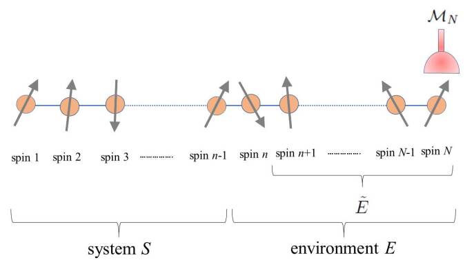
Figure 1: The spin chain, from spin $1$ to spin $N$. Each spin interacts with its nearest neighbors through the Hamiltonian in Eq. (2), with all $b_{j}=0$. The measurement $\mathcal{M}_{N}$ is performed on spin $N$, at $t=0$. We divide the spin chain into two parts: from spin $1$ to spin $n-1$ as the system $S$, and from spin $n$ to spin $N$ as the environment $E$. In addition, we divide the environment $E$ into two parts: spin $n$ and $\tilde{E}$.

Lemma 2.

If $A_{k}$, in Eq. (8), can be decomposed as Eq. (16), with $\mathrm{Tr}_{\tilde{E}}(C^{(0)})=0$ and $\mathrm{Tr}_{\tilde{E}}(C^{(3)})=0$, then we have similarly

$$A_{k+1}=D^{(0)}\otimes I_{n}+D^{(1)}\otimes X_{n}+D^{(2)}\otimes Y_{n}+D^{(3)}\otimes Z_{n},$$ (17)

with $\mathrm{Tr}_{\tilde{E}}(D^{(0)})=0$ and $\mathrm{Tr}_{\tilde{E}}(D^{(3)})=0$.

Proof. As we have seen after Eq. (16), when $\mathrm{Tr}_{\tilde{E}}(C^{(3)})=0$, then $\mathrm{Tr}_{E}(A_{k+1})=0$. So, $\mathrm{Tr}_{\tilde{E}}(D^{(0)})=0$.

In order to show that $\mathrm{Tr}_{\tilde{E}}(D^{(3)})=0$, we first decompose the Hamiltonian in Eq. (2), with all $b_{j}=0$, as

$$H=Z_{n-1}\otimes Z_{n}+Z_{n}\otimes Z_{n+1}+I_{n}\otimes\tilde{H},$$ (18)

where $\tilde{H}$ is a Hermitian operator on the other spins, except spin $n$. Using Eqs. (16) and (18), and since $A_{k+1}=[A_{k},H]$, we conclude that $D^{(3)}$ in Eq. (17) is

$$D^{(3)}=[C^{(0)},Z_{n-1}]+[C^{(0)},Z_{n+1}]+[C^{(3)},\tilde{H}].$$ (19)

As stated after Eq. (16), $C^{(0)}$ is a linear operator on $\mathcal{H}_{S}\otimes\mathcal{H}_{\tilde{E}}$, where $\mathcal{H}_{\tilde{E}}$ denotes the Hilbert space of $\tilde{E}$, such that $\mathrm{Tr}_{\tilde{E}}(C^{(0)})=0$. In addition, $Z_{n-1}$ and $Z_{n+1}$ are Hermitian operators on $\mathcal{H}_{S}\otimes\mathcal{H}_{\tilde{E}}$ as $H_{S}^{\prime}\otimes I_{\tilde{E}}$ and $I_{S}\otimes H^{\prime}_{\tilde{E}}$, respectively, where $H_{S}^{\prime}$ is a Hermitian operator on $\mathcal{H}_{S}$, $I_{\tilde{E}}$ is the identity operator on $\mathcal{H}_{\tilde{E}}$ and $H^{\prime}_{\tilde{E}}$ is a Hermitian operator on $\mathcal{H}_{\tilde{E}}$. So, using Lemma 1 (after replacing $E$ with $\tilde{E}$), we conclude that $\mathrm{Tr}_{\tilde{E}}([C^{(0)},Z_{n-1}])=0$ and $\mathrm{Tr}_{\tilde{E}}([C^{(0)},Z_{n+1}])=0$.

Similarly, $C^{(3)}$ is a linear operator on $\mathcal{H}_{S}\otimes\mathcal{H}_{\tilde{E}}$ such that $\mathrm{Tr}_{\tilde{E}}(C^{(3)})=0$. In addition, $\tilde{H}$ is a Hermitian operators on $\mathcal{H}_{S}\otimes\mathcal{H}_{\tilde{E}}$. Since the Hamiltonian in Eq. (2) only includes the nearest neighbors interaction, $\tilde{H}$ includes terms as $H_{S}^{\prime}\otimes I_{\tilde{E}}$ or $I_{S}\otimes H^{\prime}_{\tilde{E}}$. So, again using Lemma 1, we conclude that $\mathrm{Tr}_{\tilde{E}}([C^{(3)},\tilde{H}])=0$. Therefore, we have shown that $\mathrm{Tr}_{\tilde{E}}(D^{(3)})=0$. $\ \ \qquad\qquad\qquad\quad\qquad\qquad\blacksquare$

Let us decompose the linear operator $R=A_{0}$, in Eq. (5), as Eq. (16):

$$R=R^{(0)}\otimes I_{n}+R^{(1)}\otimes X_{n}+R^{(2)}\otimes Y_{n}+R^{(3)}\otimes Z_{n}.$$ (20)

Now, since in Eq. (5) we have chosen $\rho_{SE}$ and $\sigma_{SE}$ such that their reduced states of the system $S$ are the same, we have $\mathrm{Tr}_{\tilde{E}}(R^{(0)})=0$. Lemma 2 shows that if we choose $R$ appropriately, i.e., if in addition $\mathrm{Tr}_{\tilde{E}}(R^{(3)})=0$, then, for arbitrary $k$ in Eq. (16), we have $\mathrm{Tr}_{\tilde{E}}(C^{(0)})=0$. Therefore, $\mathrm{Tr}_{E}(A_{k})=0$, for all $k$ in Eq. (8), and so, for all the times $t$, the reduced dynamics of the system $S$ remains the same, for both initial state of the system-environment $\rho_{SE}$ and $\sigma_{SE}$ in Eq. (5).

We choose the initial state of the system-environment at $t=0$ as

$$\rho_{SE}=\rho_{S\tilde{E}}\otimes\rho_{n},$$ (21)

where $\rho_{S\tilde{E}}$ is an arbitrary state on $\mathcal{H}_{S}\otimes\mathcal{H}_{\tilde{E}}$, and $\rho_{n}$ is an arbitrary state of spin $n$, in the $xy$ plane of the Bloch sphere 1 :

$$\rho_{n}=\frac{1}{2}(I_{n}+r_{x}X_{n}+r_{y}Y_{n}),$$ (22)

where $r_{x}$ and $r_{y}$ are real coefficients. So, $\rho_{SE}$ in Eq. (21) can be decomposed as

$$\rho_{SE}=\bar{R}^{(0)}\otimes I_{n}+\bar{R}^{(1)}\otimes X_{n}+\bar{R}^{(2)}\otimes Y_{n},$$ (23)

where $\bar{R}^{(\mu)}$ are Hermitian operators on $\mathcal{H}_{S}\otimes\mathcal{H}_{\tilde{E}}$.

If at time $t=0$ we perform an instantaneous measurement $\mathcal{M}_{N}$ on spin $N$, then the whole state of the system-environment, at the same time $t=0$, changes to

$$\sigma_{SE}=\hat{R}^{(0)}\otimes I_{n}+\hat{R}^{(1)}\otimes X_{n}+\hat{R}^{(2)}\otimes Y_{n}$$ (24)

$$=\rho_{SE}+R,$$

where $\hat{R}^{(\mu)}=\mathrm{id}_{r}\otimes\mathcal{M}_{N}(\bar{R}^{(\mu)})$. The map $\mathcal{M}_{N}$ is a trace-preserving (completely positive) map on spin $N$, and $\mathrm{id}_{r}$ is the identity map on the rest of the spins, except spin $n$ and spin $N$.

Now, if we decompose $R$ in Eq. (24) as Eq. (20), we have

$$R^{(\mu)}=\hat{R}^{(\mu)}-\bar{R}^{(\mu)}.$$ (25)

Since $\mathcal{M}_{N}$ is trace-preserving, we have $\mathrm{Tr}_{\tilde{E}}(R^{(0)})=0$. In other words, performing the measurement $\mathcal{M}_{N}$ on spin $N$, which is a part of the environment $E$, does not affect (the reduced state of) the system $S$, and so $\mathrm{Tr}_{E}(R)=0$, which results in $\mathrm{Tr}_{\tilde{E}}(R^{(0)})=0$.

In addition, we have chosen $\rho_{SE}$ in Eq. (23) such that $\bar{R}^{(3)}=0$. So, $\hat{R}^{(3)}$ in Eq. (24) and $R^{(3)}$ in Eq. (25) are also zero. Therefore, the operator $R=A_{0}$ in Eq. (24) has all the requirements needed in Lemma 2. Consequently, $\mathrm{Tr}_{E}(A_{k})=0$, for all $k$ in Eq. (8), and so the reduced state of the system $S$, for both initial states $\rho_{SE}$ in Eq. (23) and $\sigma_{SE}$ in Eq. (24) remains the same for all $t$.

In other words, whether or not we perform the measurement $\mathcal{M}_{N}$ on spin $N$ at $t=0$, and so whether the initial state of the whole spin chain, at $t=0$, is $\sigma_{SE}$ in Eq. (24) or $\rho_{SE}$ in Eq. (23), the reduced dynamics of the system $S$ (and so spin $1$ as a part of $S$) remains the same for all $t\geq 0$. Therefore, spin $1$ will never become aware of performing the measurement $\mathcal{M}_{N}$ on spin $N$.

Let us summarize our main result of this paper, in the following Proposition:

Proposition 2.

Consider a spin chain, from spin $1$ to spin $N$, which interact through the Hamiltonian $H=\sum_{j=1}^{N-1}Z_{j}\otimes Z_{j+1}$. We divide this spin chain into two parts: We consider spins $1$ to $n-1$ as the system $S$, and spins $n$ to $N$ as the environment $E$. Next, we choose the initial state of the whole spin chain, at $t=0$, as $\rho_{SE}$ in Eq. (23). Performing an instantaneous trace-preserving measurement $\mathcal{M}_{N}$ on spin $N$ changes the initial state of spin chain to $\sigma_{SE}$ in Eq. (24), at the same time $t=0$. But, the reduced state of the system $S$ remains unchanged at this initial instant $t=0$, i.e., $\mathrm{Tr}_{E}(\sigma_{SE})=\mathrm{Tr}_{E}(\rho_{SE})$. Using Lemma 2, we have shown that Eq. (7) is satisfied, and so the reduced state of the system $S$, for all the times, remains the same, for both initial states $\sigma_{SE}$ and $\rho_{SE}$. In other words, performing or not performing the measurement $\mathcal{M}_{N}$ on spin $N$, at $t=0$, does not affect the reduced dynamics of the system $S$, for any $t\geq 0$. Therefore, any spin in the system $S$, including spin $1$, will never become aware of performing the measurement $\mathcal{M}_{N}$ on spin $N$.

Remark 1.

The minimum $N$ for which the results of this section can be applied is $N=3$. Then, spin $1$ is the system $S$, $n=2$ and spin $3$ is the subspace $\tilde{E}$.

Remark 2.

In order to achieve Proposition 2, we only require that initial $\rho_{SE}$ be as Eq. (23). The state given in Eq. (21) is only an example of such $\rho_{SE}$.

Let us end this section with the following point. The assumption that the measurement $\mathcal{M}_{N}$ is performed instantaneously can be relaxed as the following: Assume that the measurement $\mathcal{M}_{N}$, on spin $N$, lasts from $t=0$ to $t=\delta$. Denote the initial state of the whole spin chain, at $t=0$, as $\omega_{SE}$. So, $\rho_{SE}=\exp(-iH\delta)\omega_{SE}$ gives the state of the spin chain, after the time interval $\delta$, if the measurement $\mathcal{M}_{N}$ were not performed. In addition, denote the state of the spin chain at $t=\delta$, right after the measurement $\mathcal{M}_{N}$, as $\sigma_{SE}$. Now, if we have $\sigma_{SE}=\mathrm{id}_{r}\otimes\mathcal{M}_{N}(\rho_{SE})$, where $\mathcal{M}_{N}$ is a linear trace-preserving map on spin $N$, and $\mathrm{id}_{r}$ is the identity map on the rest of the spins, then we can follow a similar line of reasoning, as given from Eq. (23) onward, to show that, choosing $\rho_{SE}$ appropriately, spin $1$ will never become aware of performing $\mathcal{M}_{N}$ on spin $N$.

IV Summary and discussion

Considering a spin chain, we have shown that if we choose the initial state and the Hamiltonian of the spin chain appropriately, then the reduced state of spin $1$ is never affected by the instantaneous measurement $\mathcal{M}_{N}$ performed on spin $N$.

Assuming that the whole information in spin $1$ is what can be extracted from its reduced state, we can interpret the above result as the following: No information of performing $\mathcal{M}_{N}$ on spin $N$ will achieve spin $1$.

It is worth noting that such kind of assumption is, in fact, the basis of the Deutsch–Hayden approach to quantum mechanics 2 . They have assumed that the information is local. So, the information in a part of a composite system is what can be extracted from its reduced state.

The next issue, which we should address, is whether instantaneous measurement is possible or not. According to the text-book quantum mechanics, instantaneous measurement seems necessary: Consider a particle with a spatially widespread wave function, which is detected in a localized detector. It seems that we should accept that its wave function is collapsed instantaneously, from the pre-measurement widespread one, to a localized one, which is confined within the detector.

However, in many cases, one can model the measurement procedure as the following 15 . Step 1: The quantum system $Q$, which we want to measure the observable $\mathcal{M}_{Q}$ (with projectors $\Pi_{l}$) on it, interacts with another system, the probe $P$, such that the whole state of the system-probe $\rho_{QP}$ becomes correlated. Step 2: A projective measurement is performed on $P$, in a special basis, called the pointer states ${|l_{P}\rangle}$. Now, if the measurement result is ${|l_{P}\rangle}$, the state of the system $Q$ is left within the subspace spanned by $\Pi_{l}$.

Step 1 is deterministic. It can be modeled simply assuming that the system $Q$ and the probe $P$ interact through a unitary operator, for a period of time $\tau$, such that the initial uncorrelated state of the system-probe changes to an entangled (a correlated) one 13 ; 9 ; 11 . One can also consider more involved models, such as considering an environment $\mathcal{E}$ which interacts with $P$ 14 ; 8 , or averaging over different periods $\tau$ 12 .

Even if we assume that the probabilistic step 2 is performed instantaneously, as predicted by the standard text-book quantum mechanics, step 1 obviously takes some time. Consider the case that the initial state of the system-probe, before interacting with each other, is $|\psi_{Q}\rangle\otimes|0_{P}\rangle$. An estimate for the time needed to evolve from this initial state to the entangled state $|\phi_{QP}\rangle=\sum_{l}\Pi_{l}|\psi_{Q}\rangle\otimes|l_{P}\rangle$, is given in Ref. 9 . Also, in Ref. 8 , a lower bound on the time needed to go form the pure state $|\phi_{QP}\rangle$ to the mixed state $\rho_{QP}=\sum_{l}\Pi_{l}|\psi_{Q}\rangle\langle\psi_{Q}|\Pi_{l}\otimes|l_{P}\rangle\langle l_{P}|$ is presented. One may argue that the time needed to go from $|\phi_{QP}\rangle$ to $\rho_{QP}$, as a result of the interaction between $P$ and $\mathcal{E}$, can be considered as the time that the collapse of the wave function $|\phi_{QP}\rangle$ lasts 14 ; 15 ; 8 . But, we think that the collapse is a probabilistic event, occurred only through step 2.

However, whether our results can be applied to the case that the measurement procedure on spin $N$ includes the two above mentioned steps, and so takes some time $\delta$, is addressed in the last paragraph of the previous section. At least, when $\delta$ is sufficiently small such that $U=\exp(-iH\delta)$ can be approximated by the identity operator, our results can be used approximately, since $\rho_{SE}$ is almost the same as $\omega_{SE}$, and $\sigma_{SE}$ is approximately given by $\mathrm{id}_{r}\otimes\mathcal{M}_{N}(\omega_{SE})$.

References

(1) M. A. Nielsen and I. L. Chuang, Quantum Computation and Quantum Information (Cambridge University Press, Cambridge, England, 2000).
(3) I. Sargolzahi, Necessary and sufficient condition for the reduced dynamics of an open quantum system interacting with an environment to be linear, Phys. Rev. A 102, 022208 (2020).
(4) S. Nazifkar and I. Sargolzahi, Completely positive reduced dynamics with non-Markovian initial states, Iran. J. Phys. Res. 22, 871 (2023).
(5) E. Brüning, H. Mäkelä, A. Messina and F.
Petruccione, Parametrizations of density
matrices, J. Mod. Opt. 59, 1 (2012).
(12) N. Shettell, F. Centrone and L. P. García-Pintos,
Bounding the minimum time of a quantum measurement, arXiv:2209.06248 (2022).
(13) E. Schwarzhans, F. C. Binder, M. Huber and M. P. E. Lock, Quantum measurements and equilibration:
the emergence of objective reality via entropy maximisation, arXiv:2302.11253 (2023).