A New Low-Rank Learning Robust Quaternion Tensor Completion Method for Color Video Inpainting Problem and Fast Algorithms

Abstract

The color video inpainting problem is one of the most challenging problem in the modern imaging science. It aims to recover a color video from a small part of pixels that may contain noise. However, there are less of robust models that can simultaneously preserve the coupling of color channels and the evolution of color video frames. In this paper, we present a new robust quaternion tensor completion (RQTC) model to solve this challenging problem and derive the exact recovery theory. The main idea is to build a quaternion tensor optimization model to recover a low-rank quaternion tensor that represents the targeted color video and a sparse quaternion tensor that represents noise. This new model is very efficient to recover high dimensional data that satisfies the prior low-rank assumption. To solve the case without low-rank property, we introduce a new low-rank learning RQTC model, which rearranges similar patches classified by a quaternion learning method into smaller tensors satisfying the prior low-rank assumption. We also propose fast algorithms with global convergence guarantees. In numerical experiments, the proposed methods successfully recover color videos with eliminating color contamination and keeping the continuity of video scenery, and their solutions are of higher quality in terms of PSNR and SSIM values than the state-of-the-art algorithms.

I Introduction

Many applications of multi-dimensional data (tensor data) are becoming popular. For instance, color videos or images can be seen as 3-mode or 2-mode quaternion data. With its capacity to capture the fundamental substructures and color information, quaternion tensor-based modeling is an obvious choice to solve color video processing problems. A modern and challenging problem is color video inpainting, which aims to recover a color video from a sampling of its pixels that may contain noise. In mathematical language, this problem is robust quaternion tensor completion (RQTC) problem. There are currently less of methods to solve this problem because it is difficult to preserve the coupling of color channels and the evolution of color video frames. In this paper, we present new robust quaternion tensor completion (RQTC) models to solve this challenging problem.

For a single color image, the robust quaternion matrix completion (RQMC) method proposed in [10] theoretically solved the color image inpainting under the incoherence conditions. Chen and Ng [2] proposed a cross-channel weight strategy and analysed the error bound of RQMC problem. Xu et al. [23] proposed a new model to combine deep prior and low-rank quaternion prior in color image processing. A generous amount of practical applications indicate that RQMC can completely recover the color images of which low-frequency information dominates, but it fails to recover the color image of which high-frequency information dominates. To inpaint color images in the latter case, a new nonlocal self-similarity (NSS) based RQMC was introduced in [8] to compute an optimal approximation to the color image. The main idea is to gather similar patches into several color images of small size that mainly contain low-frequency information. This NSS-based RQMC uses the distance function to find low-rank structures of color images. It is also applied to solve color video inpainting problems and achieves color videos of high quality. However, it overlooks the global information that reflects the potential relation of continuous frames. So we need to build a quaternion tensor-based model for color video inpainting.

Recall that several famous real tensor decompositions [12] serve as the foundation of modern robust tensor completion (RTC) approaches. For instance, Liu et al. [14] presented a sum-of-nuclear-norms (SNN) as tensor rank in the RTC model. This representation depends on the Tucker decomposition [20] and SNN model is proved with an exact recovery guarantee in [6]. Gao and Zhang [4] proposed a novel nonconvex model with $\ell_{p}$ norm to solve RTC problem. Jiang et al. [11] presented a data-adaptive dictionary to determine relevant third-order tensor tubes and established a new tensor learning and coding model. Ng et al. [18] proposed a novel unitary transform method that is very efficient by using similar patches strategy to form a third-order sub-tensor. Wang et al. [21] recovered tensors by two new tensor norms. Zhao et al. [27] proposed an equivalent nonconvex surrogates of RTC problem and analysed the recovery error bound. These RTC methods have been successfully applied in color image or video processing. However, RTC models regard color images as 3-mode real tensors [13, 16] and color videos as 4-mode real tensors [7] and thus, they usually independently process three color channels and ignore the mutual connection among channels.

Since quaternion has ${\bf i},{\bf j},{\bf k}$ three imaginary parts, a color pixel can be seen as a pure quaternion. Based on quaternion representation and calculation, the color information can be preserved in the color image processing. A low-rank quaternion tensor completion method (LRQTC) was proposed in [17]. It cannot deal with the noisy or corrupted problem since it only contains a low-rank regularization term. By introducing a new sparsity regularization term into the subject function, we propose a new RQTC method for color video inpainting with missing and corrupted pixels. There are two new models. One is a robust quaternion tensor completion (RQTC) model, which recovers color videos from a global view. It is essentially in the form of a quaternion minimization problem with rank and $\ell_{1}$ norm two regularization terms. The other is a low-rank learning RQTC (LRL-RQTC) model. We intend to learn similar information to form low-rank structure and prove the numerical low-rank property in theory. Under the view of numerical linear algebra, the principal components computed by two-dimensional principal component analysis (2DPCA) [24] span an optimal subspace on which projected samples are maximally scattered. Meanwhile, low-rank approximations of original samples can be simultaneously reconstructed from such low-dimension projections. Recently, 2DPCA is generalized to quaternion, named by two-dimensional quaternion principal component analysis (2DQPCA), in [9] and 2DQPCA performs well on color image clustering. 2DQPCA and the variations extract features from training data and utilize these features to project training and testing samples into projections of low dimensions for efficient use of available computational resources. We find that 2DQPCA is a good learning method to extract low-rank structure from quaternion tensors. So we apply 2DQPCA method to learn the low-rank structure adaptively.

The highlights are as follows:

• We present a novel RQTC method for color video inpainting problem with missing and corrupted pixels and derive the exact recovery theorem. This method can simultaneously preserve the coupling of color channels and the evolution of color video frames.

• We firstly introduce the 2DQPCA technology into color video inpainting to learn the low-rank structures of quaternion tensors and present a new low-rank learning RQTC model. Moreover, the numerical low-rank property is proved in theory.

• We design new RQTC and LRL-RQTC algorithms based on the alternating direction method of multipliers (ADMM) framework and apply them to solve color video inpainting problems with missing or noisy pixels. The color videos computed by the newly proposed algorithms are of higher quality in terms of PSNR and SSIM values than those by the state-of-the-art algorithms.

This paper is organized as follows. In Section II, we introduce preliminaries about quaternion matrix and the quaternion matrix completion method. In Section III, we present new robust quaternion tensor completion and low-rank learning robust quaternion tensor completion models, including solving procedure, sufficient conditions for precise recovery, convergence analysis, 2DQPCA-based classification technology to learn low-rank information, and theoretical analysis of numerical low-rank. In Section IV, we propose experimental results of color video inpainting, which indicate the advantages of the newly proposed methods on quality of restorations. In Section V, we conclude the paper and present prospects.

II Preliminaries

Several necessary results about quaternion matrices are recalled in this section.

II-A Quaternion matrix

Let $\mathbb{Q}$ denotes the set of quaternion and a quaternion ${\bf a}$ has one real part $a_{0}\in\mathbb{R}$, three imaginary parts $a_{1},a_{2},a_{3}\in\mathbb{R}$ and is expressed as ${\bf a}=a_{0}+a_{1}{\bf i}+a_{2}{\bf j}+a_{3}{\bf k},{\bf i}^{2}={\bf j}^{2}={\bf k}^{2}={\bf i}{\bf j}{\bf k}=-1$ [5]. A symbol of boldface is used to express quaternion scalar, vector, matrix or tensor. A quaternion matrix ${\bf A}=A_{0}+A_{1}{\bf i}+A_{2}{\bf j}+A_{3}{\bf k}\in\mathbb{Q}^{m\times n}$ with $A_{0},\ldots,A_{3}\in\mathbb{R}^{m\times n}$. If $A_{0}=0$ and $A_{1},A_{2},A_{3}\neq 0$, ${\bf A}$ is named by a purely imaginary quaternion matrix. The quaternion shrinkage function shrinkQ is defined in [8] by:

$$\texttt{shrinkQ}({\bf A},\tau) =\underset{{\bf A}}{\operatorname{arg~{}min}}~{}~{}\frac{1}{2}\|{\bf A}-{\bf Z}\|_{F}^{2}+\tau\left\|{\bf A}\right\|_{1},$$ (1)

$$=\![\texttt{signQ}({\bf a}_{ij})\max(\texttt{absQ}({\bf a}_{ij})-\tau,0)]$$

where $\tau>0$, $\texttt{absQ}({\bf A}):=[|{\bf a}_{ij}|]$ and

$$\texttt{signQ}({\bf a}_{ij}):=\left\{\begin{array}[]{ll}{\bf a}_{ij}/|{\bf a}_{ij}|,&\text{if}~{}~{}|{\bf a}_{ij}|\neq 0;\\ 0,&\text{otherwise.}\end{array}\right.$$

Suppose ${\bf A}={\bf U}\Sigma{\bf V}^{*}$ is the singular value decomposition and denote $\{\sigma_{j},{\bf u}_{j},{\bf v}_{j}\}$ by the singular triplets of a quaternion matrix ${\bf A}\in\mathbb{Q}^{m\times n}$. The quaternion singular thresholding function approxQ is defined in [8] by:

$$\texttt{approxQ}({\bf A},\tau) =\underset{{\bf A}}{\operatorname{arg~{}min}}~{}~{}(\left\|{{\bf A}}\right\|_{\ast}+\frac{1}{2\tau}\|{\bf A}-{\bf Y}\|_{F}^{2})$$ (2)

$$={\bf U}\texttt{diag}(\sigma_{1},\cdots,\sigma_{k},0,\cdots,0){\bf V}^{*},\tau>0,$$

where $\sigma_{1}\geq\cdots\geq\sigma_{k}>\tau$ and the singular values $\sigma_{j}<\tau$ are substituted by zeros. Quaternion matrix norms are defined by $\left\|{\bf A}\right\|_{1}:=\sum\limits_{i=1}^{m}\sum\limits_{j=1}^{n}\left|{\bf a}_{ij}\right|$, $\left\|{\bf A}\right\|_{\infty}:=\max\limits_{i,j}\left|{\bf a}_{ij}\right|$, $\left\|{\bf A}\right\|_{F}=\sqrt{\sum\limits_{i=1}^{m}\sum\limits_{j=1}^{n}\left|{\bf a}_{ij}\right|^{2}}:=\sqrt{\operatorname{Tr}\left({\bf A}^{*}{\bf A}\right)}$, and $\|{\bf A}\|_{*}:=\sum\limits_{i=1}^{r}\sigma_{i}$.

II-B Robust quaternion matrix completion method

A low-rank quaternion matrix ${\bf L}_{0}$ can be recovered completely from an observed quaternion matrix ${\bf X}=\mathcal{P}_{\Omega}({\bf L}_{0}+{\bf S}_{0})$ by the RQMC method [10], where ${\bf S}_{0}$ is a noisy matrix and $\mathcal{P}_{\Omega}$ is a random sampling operator:

$$\mathcal{P}_{\Omega}({\bf X})=\left\{\begin{array}[]{cc}{\bf x}_{i,j},&(i,j)\in\Omega,\\ 0,&\text{otherwise}.\end{array}\right.$$

By [10, Theorem 2], if the sufficient conditions are satisfies, ${\bf L}_{0}$ can be exactly computed by solving the following minimization problem with $\lambda=\frac{1}{\rho n_{(1)}}$,

$$\begin{array}[]{rl}\underset{\bf L,\bf S}{\min}&\left\|{\bf L}\right\|_{\ast}+\lambda\left\|{\bf S}\right\|_{1}\\ \ {\rm s.t.}&\mathcal{P}_{\Omega}\left({\bf L}+{\bf S}\right)={\bf X}.\end{array}$$ (3)

A practical QMC algorithm is given in [8, Supplementary Material]. The augmented Lagrangian function of (3) is defined by

$$\begin{array}[]{rl}\underset{{\bf L},{\bf S},{\bf P},{\bf Q}}{\min}&\left\|{\bf L}\right\|_{\ast}+\lambda\left\|{\bf S}\right\|_{1}+\frac{\mu}{2}\left\|{\bf L-\bf P+\bf Y/\mu}\right\|_{F}^{2}\\ &+\frac{\mu}{2}\left\|{\bf S-\bf Q+\bf Z/\mu}\right\|_{F}^{2}\\ \ {\rm s.t.}&\mathcal{P}_{\Omega}\left({\bf P}+{\bf Q}\right)={\bf X},\end{array}$$

where $\mu$ is the penalty parameter. The solving procedure is

$$\left\{\begin{aligned} {\bf L}^{t+1}&=\texttt{approxQ}({\bf P}^{t}-({\bf Y}/\mu)^{t},\frac{1}{\mu}),\\ {\bf Q}_{i,j}^{t+1}&=\left\{\begin{array}[]{cc}({\bf X}^{t}-{\bf P}^{t})_{i,j},&(i,j)\in\Omega,\\ ({\bf S}^{t}+{\bf Z}^{t}/\mu)_{i,j},&\text{otherwise},\end{array}\right.\\ {\bf S}^{t+1}&=\texttt{shrinkQ}({\bf Q}^{t}-({\bf Z}/\mu)^{t},\frac{\lambda}{\mu}),\\ {\bf F}_{i,j}^{t+1}&=(\mu{\bf L}^{t}+\mu{\bf X}^{t}-\mu{\bf S}^{t}+{\bf Y}^{t}-{\bf Z}^{t})_{i,j},\\ {\bf P}_{i,j}^{t+1}&=\left\{\begin{array}[]{ll}{\bf F}_{i,j}^{t+1}/2\mu,&(i,j)\in\Omega,\\ ({\bf L}^{t}+{\bf Y}^{t}/\mu)_{i,j},&\text{otherwise},\end{array}\right.\\ {\bf Y}^{t+1}&={\bf Y}^{t}+\mu({\bf L}^{t}-{\bf P}^{t}),\\ {\bf Z}^{t+1}&={\bf Z}^{t}+\mu({\bf S}^{t}-{\bf Q}^{t}).\end{aligned}\right.$$ (4)

III Robust Quaternion Tensor Completion Models and Fast Algorithms

In this section, we propose two new RQTC models to solve color video inpainting problem with partial and corrupted pixels, as well as their fast algorithms.

The boldface Euler script letters, e.g. $\boldsymbol{\mathcal{X}}$, $\boldsymbol{\mathcal{L}}$ and $\boldsymbol{\mathcal{S}}$, are used to denote quaternion tensors. Let $\boldsymbol{\mathcal{X}}\in\mathbb{Q}^{n_{1}\times n_{2}\times\cdots\times n_{k}}$ be a $k$-mode quaternion tensor. The elements of $\boldsymbol{\mathcal{X}}$ are denoted by ${\bf x}_{i_{1}i_{2}\cdots i_{k}}$, where $1\leq i_{j}\leq n_{j},j=1,\cdots,k$. A $j$-mode fiber is an $n_{j}$-dimensional column vector constructed by entries with fixing all indexes except the $j$th one, denoted by $\boldsymbol{\mathcal{X}}(i_{1},\cdots,i_{j-1},:,i_{j+1},\cdots,i_{k})$. The number of $j$-mode fibers is $\prod\limits_{i\neq j}n_{i}$. Concatenate all of $j$-mode fibers as column vectors (in dictionary order) into a quaternion matrix ${\bf X}_{(j)}\in\mathbb{Q}^{n_{j}\times\prod\limits_{i\neq j}n_{i}}$ and name it by the $j$-mode unfolding of quaternion tensor $\boldsymbol{\mathcal{X}}$. We define the ‘unfold’ function on quaternion tensor $\boldsymbol{\mathcal{X}}$ by

$$\texttt{unfold}_{j}(\boldsymbol{\mathcal{X}}):={\bf X}_{(j)},~{}~{}j=1,\cdots,k,$$ (5)

and the ‘fold’ function by

$$\texttt{fold}_{j}({\bf X}_{(j)}):=\boldsymbol{\mathcal{X}}.$$ (6)

A slice of $\boldsymbol{\mathcal{X}}$ is a quaternion matrix of the form $\boldsymbol{\mathcal{X}}(i_{1},\cdots,i_{j_{1}-1},:,i_{j_{1}+1},\cdots,i_{j_{2}-1},:,i_{j_{2}+1},\cdots,i_{k})$ with all the indexes being fixed except $j_{1}$ and $j_{2}$.

One important application of quaternion tensor is color video processing. A color video with $n_{3}$ frames can be seen as a $3$-mode quaternion tensor $\boldsymbol{\mathcal{X}}=\mathcal{R}{\bf i}+\mathcal{G}{\bf j}+\mathcal{B}{\bf k}\in{\mathbb{Q}}^{n_{1}\times n_{2}\times n_{3}}$, where $\mathcal{R}$, $\mathcal{G}$ and $\mathcal{B}\in\mathbb{R}^{n_{1}\times n_{2}\times n_{3}}$ represent the red, green and blue three channels. Mathematically, color video inpainting problem with noise is exactly the RQTC problem (with $k=3$), which will be characterized later in (7).

III-A RQTC model

Let $\boldsymbol{\mathcal{X}}\in{\mathbb{Q}}^{n_{1}\times n_{2}\times\cdots\times n_{k}}$ denotes observed quaternion tensor with missing and/or corrupted entries. Then the RQTC problem is mathematically modeled by the following minimization problem,

$$\begin{array}[]{rl}\underset{\boldsymbol{\mathcal{L}},\boldsymbol{\mathcal{S}}}{\min}&\left\|{\boldsymbol{\mathcal{L}}}\right\|_{\ast}+\lambda\left\|{\boldsymbol{\mathcal{S}}}\right\|_{1}\\ \ {\rm s.t.}&\mathcal{P}_{\Omega}\left({\boldsymbol{\mathcal{L}}}+{\boldsymbol{\mathcal{S}}}\right)=\boldsymbol{\mathcal{X}}\end{array}$$ (7)

where $\boldsymbol{\mathcal{L}}$, $\boldsymbol{\mathcal{S}}$ $\in{\mathbb{Q}}^{n_{1}\times n_{2}\times\cdots\times n_{k}}$ denote the target low-rank tensor and the sparse data, respectively. The quaternion tensor random sampling operator $\mathcal{P}_{\Omega}$ is defined by

$$(\mathcal{P}_{\Omega}[\boldsymbol{\mathcal{X}}])_{i_{1}i_{2}\cdots i_{k}}:=\left\{\begin{aligned} {\bf x}_{i_{1}i_{2}\cdots i_{k}}&,\quad(i_{1},i_{2},\cdots i_{k})\in\Omega\\ 0&,\quad\text{otherwise}.\end{aligned}\right.$$

The quaternion tensor nuclear norm and the $\ell_{1}$ norm are defined by

$$\left\|{\boldsymbol{\mathcal{L}}}\right\|_{\ast}:=\sum\limits_{j=1}^{k}\alpha_{j}\left\|{{\bf L}_{(j)}}\right\|_{\ast},~{}~{}\left\|{\boldsymbol{\mathcal{S}}}\right\|_{1}:=\left\|{{\bf S}_{(1)}}\right\|_{1}$$ (8)

where $\alpha_{j}$’s are constants satisfying $\alpha_{j}\geq 0$ and $\sum_{j=1}^{k}\alpha_{j}=1$. Here, the quaternion tensor nuclear norm is essentially a convex combination of quaternion matrix nuclear norms which are generated by unfolding the tensor along each mode. Notice that $\left\|{{\bf S}_{(1)}}\right\|_{1}=\left\|{{\bf S}_{(2)}}\right\|_{1}=\cdots=\left\|{{\bf S}_{(k)}}\right\|_{1}$.

To derive the exact RQTC theorem, we need to build the incoherence conditions of quaternion tensors.

Definition III.1.

For a quaternion tensor $\boldsymbol{\mathcal{X}}\in\mathbb{Q}^{n_{1}\times n_{2}\times\cdots\times n_{k}}$, suppose each ${\bf X}_{(j)}$ has the singular value decomposition

$${\bf X}_{(j)}={\bf U}_{j}\Sigma_{j}{\bf V}_{j}^{*},j=1,2,\cdots,k.$$

Let

$$r_{j}={\rm rank}({\bf X}_{(j)})\quad and\quad\boldsymbol{\mathcal{T}}:=\sum\limits_{j=1}^{k}\sqrt{n_{j}^{(1)}}\texttt{fold}_{j}({\bf U}_{j}{\bf V}_{j}^{*}).$$

Then the conditions of quaternion tensor incoherence with $\mu$, $n_{j}^{(1)}=\max\left(n_{j},\prod_{i\neq j}n_{i}\right)$, $n_{j}^{(2)}=\min\left(n_{j},\prod_{i\neq j}n_{i}\right)$ are as follows:

(1) $j$-mode incoherence

$$\begin{split}\underset{j}{\max}\|{\bf U}_{j}^{*}e_{i}\|^{2}\leq\frac{\mu r_{j}}{n_{j}},~{}\underset{j}{\max}\|{\bf V}_{j}^{*}e_{i}\|^{2}\leq\frac{\mu r_{j}}{\prod_{i=1,i\neq j}^{k}n_{i}},\\ \|{\bf U}_{j}{\bf V}_{j}^{*}\|_{\infty}\leq\mu\sqrt{\frac{r_{j}}{n_{j}^{(1)}n_{j}^{(2)}}},\end{split}$$ (9)

(2) mutual incoherence

$$\frac{\|\boldsymbol{\mathcal{T}}\|}{k}\leq\mu\sqrt{\frac{r_{j}}{n_{j}^{(2)}}}.$$ (10)

The condition (10) strengthens the original quaternion matrix incoherence condition (9) and keeps balance between the ranks of quaternion $\boldsymbol{\mathcal{X}}$. Indeed, define $\kappa_{j}:=\frac{r_{j}}{n_{j}^{(2)}}$ and $\kappa:=\max{\kappa_{j}}$. Clearly, a larger $\kappa$ means that even though quaternion tensor $\boldsymbol{\mathcal{X}}$ has a certain mode of low-rank but also has a mode of high rank.

Theorem III.1.

Suppose a quaternion tensor $\boldsymbol{\mathcal{L}}_{0}\in\mathbb{Q}^{n_{1}\times n_{2}\times\cdots\times n_{k}}$ meets the incoherence conditions in definition (III.1), a set $\Omega$ is uniformly distributed with cardinality $m=\rho n_{j}^{(1)}n_{j}^{(2)}$ and each observed entry is corrupted with probability $\gamma$ independently of other entries. The solution $\hat{\boldsymbol{\mathcal{L}}}$ of (7) with $\lambda=\sum\limits_{j=1}^{k}\frac{\alpha_{j}^{2}}{\sqrt{\rho n_{j}^{(1)}}}$ is exact with a probability of at least $1-cn^{-10}$, provided that

$$\rm rank({\bf L}_{0_{(j)}})\leq\frac{\rho_{r}n_{j}^{(2)}}{\mu({\rm log}n_{j}^{(1)})^{2}}\quad and\quad\gamma\leq\gamma_{s},~{}j=1,2,\cdots,k,$$

where, $c$, $\rho_{r}$ and $\gamma_{s}$ are positive numerical constants.

Proof.

Under the definition of quaternion tensor nuclear norm (8), model (7) reduces to the QMC model proposed in [10] when $\boldsymbol{\mathcal{L}}$ and $\boldsymbol{\mathcal{S}}$ reduce to quaternion matrix. Equivalently, model (7) is equal to

$$\begin{array}[]{rl}\underset{\boldsymbol{\mathcal{L}},\boldsymbol{\mathcal{S}}}{\min}&\sum\limits_{j=1}^{k}\alpha_{j}\left\|{{\bf L}_{(j)}}\right\|_{\ast}+\lambda\left\|{{\bf S}_{(1)}}\right\|_{1}\\ \ {\rm s.t.}&\mathcal{P}_{\Omega}\left({{\bf L}_{(j)}}+{{\bf S}_{(j)}}\right)={{\bf X}_{(j)}},j=1,2,\cdots,k,\end{array}$$ (11)

in which ${\bf L}_{(j)}$ and ${\bf S}_{(j)}$ are results of ‘unfold’ function (5) acted on $\boldsymbol{\mathcal{L}}$ and $\boldsymbol{\mathcal{S}}$ (we will use this notation in later models). Model (11) is a generalized QMC model by extending the first term of regularization function to the combination of $k$ nuclear norms. In other words, the model (11) can be written as

$$\begin{array}[]{rl}\underset{\boldsymbol{\mathcal{L}},\boldsymbol{\mathcal{S}}}{\min}&\sum\limits_{j=1}^{k}\alpha_{j}\left(\left\|{{\bf L}_{(j)}}\right\|_{\ast}+\lambda_{j}\left\|{{\bf S}_{(j)}}\right\|_{1}\right)\\ \ {\rm s.t.}&\mathcal{P}_{\Omega}\left({{\bf L}_{(j)}}+{{\bf S}_{(j)}}\right)={{\bf X}_{(j)}},j=1,2,\cdots,k.\end{array}$$ (12)

The parameter $\lambda$ in (11) is denoted by $\sum\limits_{j=1}^{k}\alpha_{j}\lambda_{j}$. Then (12) is a convex combination of three QMC problems, thus the solution $\hat{\boldsymbol{\mathcal{L}}}$ of (11) is exact as long as they satisfy the exact recovery conditions respectively. According to Theorem 2 in [10], we can get the conclusion. ∎

Introducing two auxiliary variables $\boldsymbol{\mathcal{P}}$ and $\boldsymbol{\mathcal{Q}}$, the augmented Lagrangian equation of problem (11) becomes

$$\begin{array}[]{rl}\underset{\boldsymbol{\mathcal{L}},\boldsymbol{\mathcal{S}},\boldsymbol{\mathcal{P}},\boldsymbol{\mathcal{Q}}}{\min}&\sum\limits_{j=1}^{k}\alpha_{j}\left\|{{\bf L}_{(j)}}\right\|_{\ast}+\lambda\left\|{{\bf S}_{(1)}}\right\|_{1}\\ &+\sum\limits_{j=1}^{k}\frac{\beta_{j}}{2}\|{\bf L}_{(j)}-{\bf P}_{(j)}+{\bf Y}_{(j)}/\beta_{j}\|_{F}^{2}\\ &+\frac{\mu}{2}\|{\bf S}_{(1)}-{\bf Q}_{(1)}+{\bf Z}_{(1)}/\mu\|_{F}^{2}\\ \ {\rm s.t.}&\mathcal{P}_{\Omega}\left({\boldsymbol{\mathcal{P}}}+{\boldsymbol{\mathcal{Q}}}\right)={\boldsymbol{\mathcal{X}}}.\end{array}$$ (13)

where $\beta_{j}$ and $\mu$ are penalty parameters, ${\bf Y}_{(j)}$ and ${\bf Z}_{(j)}$ are results of ‘unfold’ function (5) acted on two Lagrange multipliers $\boldsymbol{\mathcal{Y}}$ and $\boldsymbol{\mathcal{Z}}$ that are two quaternion tensors. Now, we design an optimization algorithm to solve (13) based on the ADMM framework. Problem (13) can be converted to two-block subproblems and each one contains two unknown variables:

$[\boldsymbol{\mathcal{S}},~{}\boldsymbol{\mathcal{P}}]$ subproblem:

$$\underset{\boldsymbol{\mathcal{S}}}{\min}~{}~{}\lambda\left\|{{\bf S}_{(1)}}\right\|_{1}+\frac{\mu}{2}\|{\bf S}_{(1)}-{\bf Q}_{(1)}+{\bf Z}_{(1)}/\mu\|_{F}^{2},$$

$$\underset{\boldsymbol{\mathcal{P}}}{\min}~{}~{}\|{\bf L}_{(j)}-{\bf P}_{(j)}+{\bf Y}_{(j)}/\beta_{j}\|_{F}^{2},~{}\!\!{\rm s.t.}~{}~{}\mathcal{P}_{\Omega}\left({\boldsymbol{\mathcal{P}}}+{\boldsymbol{\mathcal{Q}}}\right)={\boldsymbol{\mathcal{X}}}.$$

$[\boldsymbol{\mathcal{L}},~{}\boldsymbol{\mathcal{Q}}]$ subproblem:

$$\underset{\boldsymbol{\mathcal{L}}}{\min}~{}~{}\!\!\!\!\sum\limits_{j=1}^{k}(\alpha_{j}\left\|{{\bf L}_{(j)}}\right\|_{\ast}+\frac{\beta_{j}}{2}\|{\bf L}_{(j)}-{\bf P}_{(j)}+{\bf Y}_{(j)}/\beta_{j}\|_{F}^{2}),$$

$$\underset{\boldsymbol{\mathcal{Q}}}{\min}~{}~{}\!\!\!\!|{\bf S}_{(1)}-{\bf Q}_{(1)}+{\bf Z}_{(1)}/\mu\|_{F}^{2},~{}~{}\!\!{\rm s.t.}~{}~{}\mathcal{P}_{\Omega}\left({\boldsymbol{\mathcal{P}}}+{\boldsymbol{\mathcal{Q}}}\right)={\boldsymbol{\mathcal{X}}}.$$

By these formulae, the minimization problems of quaternion tensors are equivalently converted into the minimization problems of quaternion matrices. It seems that they can be feasibly solved by the QMC iteration (4). However, one obstacle is the $\boldsymbol{\mathcal{L}}$ subproblem that contains a convex combination of quaternion matrix norms. Fortunately, we find that this problem has a closed-form solution.

Theorem III.2.

The closed-form solution of $\boldsymbol{\mathcal{L}}$ subproblem is $\frac{1}{k}\sum_{j=1}^{k}{\rm\texttt{fold}}_{j}\left(\texttt{approxQ}\left({\bf P}_{(j)}-(1/\beta_{j})*{\bf Y}_{(j)},\alpha_{j}/\beta_{j}\right)\right)$.

Proof.

$\boldsymbol{\mathcal{L}}$ subproblem is

$$\underset{{\bf L}_{(j)}}{\min}~{}~{}\sum\limits_{j=1}^{k}(\alpha_{j}\left\|{{\bf L}_{(j)}}\right\|_{\ast}+\frac{\beta_{j}}{2}\|{\bf L}_{(j)}-{\bf P}_{(j)}+{\bf Y}_{(j)}/\beta_{j}\|_{F}^{2})$$

We find that the function $\sum\limits_{j=1}^{k}\alpha_{j}\left\|{{\bf L}_{(j)}}\right\|_{\ast}$ is a sum of non-negative functions $\alpha_{j}\left\|{{\bf L}_{(j)}}\right\|_{\ast}$ that are independent with each other. Then $\boldsymbol{\mathcal{L}}$ subproblem can be solved by finding minimizers of $k$ subproblems $\alpha_{j}\left\|{{\bf L}_{(j)}}\right\|_{\ast}+\frac{\beta_{j}}{2}\|{\bf L}_{(j)}-{\bf P}_{(j)}+{\bf Y}_{(j)}/\beta_{j}\|_{F}^{2}$, respectively. Suppose ${\bf L}_{(1)},{\bf L}_{(2)},\cdots,{\bf L}_{(j-1)},{\bf L}_{(j+1)},\cdots,{\bf L}_{(k)}$ have been known and ${\bf L}_{(j)}$ is the only unknown variable. The solution of subproblem about ${\bf L}_{(j)}$ is

$${\bf L}_{(j)} \!\!=\underset{{\bf L}_{(j)}}{\operatorname{arg~{}min}}~{}~{}(\alpha_{j}\left\|{{\bf L}_{(j)}}\right\|_{\ast}\!+\!\frac{\beta_{j}}{2}\|{\bf L}_{(j)}-{\bf P}_{(j)}+{\bf Y}_{(j)}/\beta_{j}\|_{F}^{2})$$

$$\!\!=\underset{{\bf L}_{(j)}}{\operatorname{arg~{}min}}~{}~{}(\frac{\alpha_{j}}{\beta_{j}}\left\|{{\bf L}_{(j)}}\right\|_{\ast}\!+\!\frac{1}{2}\|{\bf L}_{(j)}-{\bf P}_{(j)}+{\bf Y}_{(j)}/\beta_{j}\|_{F}^{2})$$

$$\!\!=\texttt{approxQ}\left({\bf P}_{(j)}-(1/\beta_{j})*{\bf Y}_{(j)},\alpha_{j}/\beta_{j}\right).$$

Here, the quaternion singular thresholding operator is employed in the computation. The derivation is entirely independent of the selection of $j$, so the mentioned minimization can be carried out for any ${\bf L}_{(j)},j={1,\cdots,k}.$

Each solution ${\bf L}_{(j)}$ is the optimal approximation of the $j$th unfolding of $\boldsymbol{\mathcal{L}}$. So the closed-form solution of $\boldsymbol{\mathcal{L}}$ subproblem is

$$\boldsymbol{\mathcal{L}}=\frac{1}{k}\sum_{j=1}^{k}\texttt{fold}_{j}\left(\texttt{approxQ}({\bf P}_{(j)}-(1/\beta_{j})*{\bf Y}_{(j)},\alpha_{j}/\beta_{j})\right).$$

∎

The other three subproblems can be solved similarly. For instance, the $\boldsymbol{\mathcal{S}}$ subproblem can be solved by the shrinkage of quaternion operator shrinkQ (1), and in fact, it has a closed-form solution:

$$\boldsymbol{\mathcal{S}}=\texttt{fold}_{1}\left(\texttt{shrinkQ}({\bf Q}_{(1)}-(1/\mu)*{\bf Z}_{(1)},\lambda/\mu)\right).$$

To summarize above analysis, we present a new RQTC algorithm in Algorithm 1 and prove its convergence in Theorem III.3.

Algorithm 1 RQTC Algorithm

1:Input:

2:An observed quaternion tensor $\boldsymbol{\mathcal{X}}\in\mathbb{Q}^{n_{1}\times n_{2}\cdots\times n_{k}}$

3:Known and unknown entries sets: $\Omega$ and $\overline{\Omega}$;

4:Initialize $\boldsymbol{\mathcal{L}}=\boldsymbol{\mathcal{X}}$, $\boldsymbol{\mathcal{S}}=\boldsymbol{\mathcal{P}}=\boldsymbol{\mathcal{Q}}=\boldsymbol{\mathcal{Y}}=\boldsymbol{\mathcal{Z}}=0$, $\mu,\lambda,\beta_{j}>0,\sum_{j=1}^{k}\alpha_{j}=1,j=1,2,\cdots,k$.

5:Output:

6:A low-rank quaternion tensor $\boldsymbol{\mathcal{L}}$.

7:A sparse quaternion tensor $\boldsymbol{\mathcal{S}}$.

8:Main loop:

9:while not converge do

10:     Update $\boldsymbol{\mathcal{S}}$ and $\boldsymbol{\mathcal{P}}$:

11:     for j = 1:k do

12:         ${\bf L}_{(j)}=\texttt{unfold}_{j}(\boldsymbol{\mathcal{L}})$; ${\bf P}_{(j)}=\texttt{unfold}_{j}(\boldsymbol{\mathcal{P}})$; d${\bf Y}_{(j)}=\texttt{unfold}_{j}(\boldsymbol{\mathcal{Y}})$;

13:         ${\bf P}_{(j)}(\Omega)=(\beta_{j}{\bf L}_{(j)}(\Omega)+\beta_{j}{\bf X}_{(j)}(\Omega)-\beta_{j}{\bf S}_{(j)}(\Omega)+{\bf Y}_{(j)}(\Omega){\bf Z}_{(j)}(\Omega))/2/\beta_{j}$;

14:         ${\bf P}_{(j)}(\overline{\Omega})={\bf L}_{(j)}(\overline{\Omega})+{\bf Y}_{(j)}(\overline{\Omega})/\beta_{j}$;

15:         $\boldsymbol{\mathcal{P}}_{j}=\texttt{fold}_{j}({\bf P}_{(j)})$;

16:     end for

17:     $\boldsymbol{\mathcal{P}}=\frac{1}{k}\sum_{j=1}^{k}\boldsymbol{\mathcal{P}}_{j};$

18:     $\boldsymbol{\mathcal{S}}=\texttt{shrinkQ}(\boldsymbol{\mathcal{Q}}-(1/\mu)*\boldsymbol{\mathcal{Z}},\lambda/\mu)$;

19:     Update $\boldsymbol{\mathcal{L}}$ and $\boldsymbol{\mathcal{Q}}$:

20:     for j = 1:k do

21:         ${\bf L}_{(j)}=\texttt{approxQ}({\bf P}_{(j)}-(1/\beta_{j})*{\bf Y}_{(j)},\alpha_{j}/\beta_{j})$;

22:         $\boldsymbol{\mathcal{L}}_{j}=\texttt{fold}_{j}({\bf L}_{(j)})$;

23:     end for

24:     $\boldsymbol{\mathcal{L}}=\frac{1}{k}$$\sum_{j=1}^{k}\boldsymbol{\mathcal{L}}_{j};$

25:     $\boldsymbol{\mathcal{Q}}(\Omega)=\boldsymbol{\mathcal{X}}(\Omega)-\boldsymbol{\mathcal{P}}(\Omega)$; $\boldsymbol{\mathcal{Q}}(\overline{\Omega})=\boldsymbol{\mathcal{S}}(\overline{\Omega})+\boldsymbol{\mathcal{Z}}(\overline{\Omega})/\mu$;

26:     Update $\boldsymbol{\mathcal{Y}}$ and $\boldsymbol{\mathcal{Z}}$:

27:     $\boldsymbol{\mathcal{Y}}=\boldsymbol{\mathcal{Y}}+\mu*(\boldsymbol{\mathcal{L}}-\boldsymbol{\mathcal{P}})$; $\boldsymbol{\mathcal{Z}}=\boldsymbol{\mathcal{Z}}+\mu*(\boldsymbol{\mathcal{S}}-\boldsymbol{\mathcal{Q}})$;

28:end while

Theorem III.3.

Algorithm 1 exactly convergences to the optimal solution $(\boldsymbol{\mathcal{L}}^{*},\boldsymbol{\mathcal{S}}^{*})$ of problem (11).

Proof.

Since all of the matrices mentioned in (13) are quaternion matrices, we reformulate them to real forms. Taking ${\bf L}_{(j)}=L_{0}+L_{1}{\bf i}+L_{2}{\bf j}+L_{3}{\bf k}\in\mathbb{Q}^{n_{j}\times\prod\limits_{i\neq j}n_{i}}$ as an example, we represent it with a real vector defined by $L_{c_{(j)}}=[{\rm vec}(L_{0});{\rm vec}(L_{1});{\rm vec}(L_{2});{\rm vec}(L_{3})]\in\mathbb{R}^{4n_{1}n_{2}\cdots n_{k}},$ where ${\rm vec}(L_{i})$ denotes an ($n_{1}n_{2}\cdots n_{k}$)-dimensional vector generated by stacking the columns of $L_{i}$. Thus, the quaternion model (13) is mathematically equivalent to

$$\begin{array}[]{rl}\underset{L_{c},S_{c},P_{c},Q_{c}}{\min}&\sum\limits_{j=1}^{k}\alpha_{j}\left\|{L_{c_{(j)}}}\right\|_{\ast}+\lambda\left\|{S_{c_{(1)}}}\right\|_{1}\\ &+\sum\limits_{j=1}^{k}\frac{\beta_{j}}{2}\|L_{c_{(j)}}-P_{c_{(j)}}+Y_{c_{(j)}}/\beta_{j}\|_{F}^{2}\\ &+\frac{\mu}{2}\|S_{c_{(1)}}-Q_{c_{(1)}}+Z_{c_{(1)}}/\mu\|_{F}^{2}\\ {\rm s.t.}&\mathcal{P}_{\Omega}\left({P_{c}}+{Q_{c}}\right)={X_{c}}.\end{array}$$ (14)

Problem (14) is a minimization problem about real variables. For clarification, we define the object function by

$$F\left(\left[\begin{array}[]{c}P_{c}\\ S_{c}\end{array}\right]\!\!,\!\!\left[\begin{array}[]{c}L_{c}\\ Q_{c}\end{array}\right]\!\!,\!\!\left[\begin{array}[]{c}Y_{c}\\ Z_{c}\end{array}\right]\right)\!:=\sum\limits_{j=1}^{k}\alpha_{j}\left\|{L_{c_{(j)}}}\right\|_{\ast}+\lambda\left\|{S_{c_{(1)}}}\right\|_{1}+$$

$$\sum\limits_{j=1}^{k}\!\frac{\beta_{j}}{2}\!\|L_{c_{(j)}}\!\!-\!\!P_{c_{(j)}}+Y_{c_{(j)}}/\beta_{j}\|_{F}^{2}+\frac{\mu}{2}\|S_{c_{(1)}}\!-\!Q_{c_{(1)}}+Z_{c_{(1)}}/\mu\|_{F}^{2}.$$

From [10, Proposition 2], the convex envelope of the function $\phi({\bf X})=\rm rank({\bf X})$ on $S:=\{{\bf X}\in\mathbb{Q}^{n_{1}\times n_{2}}|\|{\bf X}\|\leq 1\}$ can be expressed as

$$\phi_{envo}({\bf X})=\|{\bf X}\|_{\ast}.$$

Therefore, the nuclear function $\|\cdot\|_{\ast}$ is convex and closed. On the other hand, the $\ell_{1}$ function $\|\cdot\|_{1}$ is obviously convex and closed. Under this circumstance, the optimization problem (14) fits the framework of ADMM. We can iteratively update all variables as follows:

$$\left[\begin{array}[]{c}P_{c}^{(t+1)}\\ S_{c}^{(t+1)}\end{array}\!\right] =\underset{P_{c},S_{c}}{\operatorname{arg~{}min}}~{}\!F\left(\left[\begin{array}[]{c}L_{c}^{(t)}\\ Q_{c}^{(t)}\end{array}\!\!\right]\!,\!\left[\begin{array}[]{c}P_{c}\\ S_{c}\end{array}\!\right]\!,\!\left[\begin{array}[]{c}Y_{c}^{(t)}\\ Z_{c}^{(t)}\end{array}\!\!\right]\!\right),$$

$$\left[\begin{array}[]{c}L_{c}^{(t+1)}\\ Q_{c}^{(t+1)}\end{array}\!\right] =\underset{L_{c},Q_{c}}{\operatorname{arg~{}min}}~{}\!F\left(\left[\begin{array}[]{c}L_{c}\\ Q_{c}\end{array}\!\!\right]\!,\!\left[\begin{array}[]{c}P_{c}^{(t+1)}\\ S_{c}^{(t+1)}\end{array}\!\!\right]\!,\!\left[\begin{array}[]{c}Y_{c}^{(t)}\\ Z_{c}^{(t)}\end{array}\!\!\right]\!\right),$$

$$\left[\begin{array}[]{c}Y_{c}^{(t+1)}\\ Z_{c}^{(t+1)}\end{array}\!\!\right] =\left[\begin{array}[]{c}Y_{c}^{(t)}+\mu(L_{c}^{(t+1)}-P_{c}^{(t+1)})\\ Z_{c}^{(t)}+\mu(S_{c}^{(t+1)}-Q_{c}^{(t+1)})\end{array}\!\!\right].$$

Here, we denote $\left[\begin{array}[]{c}P_{c}\\ S_{c}\end{array}\right],\left[\begin{array}[]{c}L_{c}\\ Q_{c}\end{array}\right]$ and $\left[\begin{array}[]{c}Y_{c}\\ Z_{c}\end{array}\right]$ by $x$,$y$ and $z$, respectively. Then the above equation is consistent with the following equations in [1]:

$$x^{(t+1)} =\underset{x}{\operatorname{arg~{}min}}~{}F(x,z^{(t)},y^{(t)}),$$

$$z^{(t+1)} =\underset{x}{\operatorname{arg~{}min}}~{}F(x^{(t+1)},z,y^{(t)}),$$

$$y^{(t+1)} =y^{(t)}+\mu(Ax^{(t+1)}+Bz^{(t+1)}-c).$$

As a result, this falls essentially in the two-block ADMM framework and the convergence is theoretically guaranteed according to [1]. ∎

Remark III.1.

It is worth mentioning that this model performs better than the real tensor completion model, because the intrinsic color structures are totally retained during the computation process for the quaternion tensor, while unfold process may completely obliterate the three channels of color pixel.

Remark III.2.

A color image can be seen as a color video with only one frame and its representation is a quaternion matrix. That is, if $n_{3}=1$ then a 3-mode quaternion tensor $\boldsymbol{\mathcal{X}}$ reduces to a quaternion matrix ${\bf X}$. So the proposed RQTC method is surely a generalization of the QMC method [10]. The incoherence conditions and the assumption of low-rank and sparsity for robust quaternion tensor recovery problem surely cover those in [10, Theorem 2] for robust quaternion matrix quaternion recovery problems.

Remark III.3.

In model (7), the definitions of quaternion tensor nuclear norm and $\ell_{1}$ norm in (8) are inspired by [14], in which the SNN is established as the nuclear norm for real tensors.

In the above, we have presented a novel RQTC model with the exact recovery theorem and a new ADMM-based algorithm with a convergence proof. They are feasible and efficient to restore quaternion tensors from partial and/or corrupted entries under the condition that the assumption of Theorem III.1 is satisfied. However, the low-rank condition sometimes does not hold in practical applications. For instance, quaternion tensor that represents color video is of high-rank when color video contains high frequency information. So we need to improve our model and algorithm further.

III-B LRL-RQTC model

Now we present an improved RQTC model by introducing a low-rank learning method. For the convenience of description, we concentrate on $3$-mode quaternion tensor $\boldsymbol{\mathcal{X}}\in\mathbb{Q}^{n_{1}\times n_{2}\times n_{3}}$ that represents color video and use the engineer language instead of the mathematician language.

Since color video is often of large-scale, we set a window for searching low-rank information and denote the part of quaternion tensor in this window by adding a subscript $t$. That is, $\boldsymbol{\mathcal{X}}_{t}$ denotes a small quaternion tensor of $\boldsymbol{\mathcal{X}}$ in a fixed searching window.

Suppose we set $p$ windows totally, in other words, we divide the large tensor into $p$ smaller ones. A $3$-mode quaternion tensor is a stack of horizontal, lateral and frontal slices. We choose a series of overlapping patches of $\boldsymbol{\mathcal{X}}_{t}$ (the $t$th searching window of tensor $\boldsymbol{\mathcal{X}}$) from three kinds of slices, respectively, and classify them into $\ell_{j}$ classes $(j=1,2,3)$. Then we vectorize each patch of the $s$th class ($1\leq s\leq\ell_{j}$) and rearrange them into a quaternion matrix, denoted by $\mathscr{F}_{s}^{j}(\boldsymbol{\mathcal{X}}_{t})$, In other words, $\mathscr{F}_{s}^{j}(\boldsymbol{\mathcal{X}}_{t})$ is a low-rank quaternion matrix generated by the $s$th class of similar patches from the $j$th type of slice. Define the classification function of similar patches by

$$\mathcal{F}_{j}(\boldsymbol{\mathcal{X}}_{t}) =[\mathscr{F}_{1}^{j}(\boldsymbol{\mathcal{X}}_{t}),~{}\mathscr{F}_{2}^{j}(\boldsymbol{\mathcal{X}}_{t}),\cdots,\mathscr{F}_{\ell}^{j}(\boldsymbol{\mathcal{X}}_{t})].$$ (15)

The function is invertible and the inverse is defined by

$$\mathcal{F}_{j}^{-1}\left([\mathscr{F}_{1}^{j}(\boldsymbol{\mathcal{X}}_{t}),~{}\mathscr{F}_{2}^{j}(\boldsymbol{\mathcal{X}}_{t}),\cdots,\mathscr{F}_{\ell}^{j}(\boldsymbol{\mathcal{X}}_{t})]\right) =\boldsymbol{\mathcal{X}}_{t}.$$ (16)

Now we introduce a learning strategy into RQTC model and present a new low-rank learning robust quaternion tensor completion model (LRL-RQTC):

$$\begin{array}[]{rl}\underset{\boldsymbol{\mathcal{L}},\boldsymbol{\mathcal{S}}}{\min}&\sum\limits_{j=1}^{3}\sum\limits_{t=1}^{p}\sum\limits_{s=1}^{\ell_{j}}(\alpha_{j}\left\|{\mathscr{F}_{s}^{j}\left(\boldsymbol{\mathcal{L}}_{t}\right)}\right\|_{\ast}+\lambda_{s}\|\mathscr{F}_{s}^{j}(\boldsymbol{\mathcal{S}}_{t})\|_{1})\\ {\rm s.t.}&\mathcal{P}_{\Omega}\left({\boldsymbol{\mathcal{L}}}+{\boldsymbol{\mathcal{S}}}\right)={\boldsymbol{\mathcal{X}}}.\end{array}$$ (17)

where $\mathscr{F}_{s}^{j}$ is a mapping transformation (15). Different from the prior NSS-QMC model that uses the distance function to search similar patches, here we introduce a new 2DQPCA-based classification function and propose a new LRL-RQTC model with adaptively low-rank learning. The model (17) is a minimization issue consisting of three subproblems and independent of each other. For the convenience of the narrative, we only present the operation on the frontal slice in the following part, i.e.

$$\begin{array}[]{rl}\underset{\boldsymbol{\mathcal{L}},\boldsymbol{\mathcal{S}}}{\min}&\sum\limits_{t=1}^{p}\sum\limits_{s=1}^{\ell}\left\|{\mathscr{F}_{s}\left(\boldsymbol{\mathcal{L}}_{t}\right)}\right\|_{\ast}+\lambda_{s}\|\mathscr{F}_{s}(\boldsymbol{\mathcal{S}}_{t})\|_{1}\\ {\rm s.t.}&\mathcal{P}_{\Omega}\left({\boldsymbol{\mathcal{L}}}+{\boldsymbol{\mathcal{S}}}\right)={\boldsymbol{\mathcal{X}}}.\end{array}$$ (18)

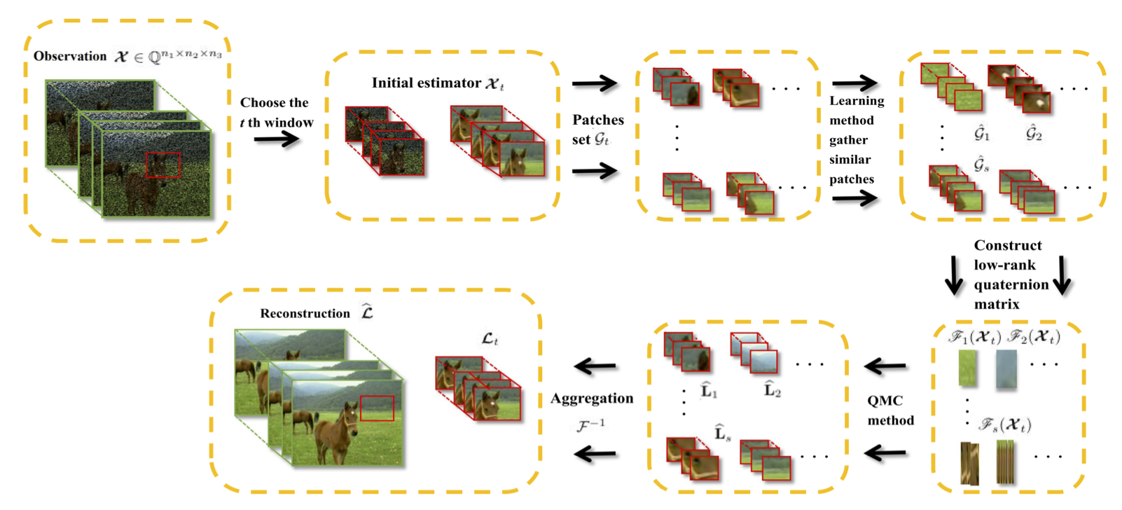
Figure 1: Flowchart of the patched-based low-rank learning method for RQTC problem.

The flowchart of the patched-based learning method is shown in Fig. 1. Firstly, choose the $t$th window $(1\leq t\leq p)$ and get $n$ overlapping patches ${\bf Y}_{t}^{(i,j)}$ with size $w\times h$ ($0<w\leq n_{1}$, $0<h\leq n_{2}$), covering each frontal slice of $\boldsymbol{\mathcal{X}}_{t}$. Then we gather them into a set $\mathcal{G}_{t}$

$$\mathcal{G}_{t}:=\{{\bf Y}_{t}^{(i,j)}\in\mathbb{Q}^{w\times h}\},$$ (19)

where $(i,j)$ denotes the location of a patch. Secondly, we set $\ell$ exemplar patches which are non-overlapping. After choosing them, we calculate their eigen subspace ${\bf V}$. Then we find a number of patches most similar to the exemplar patches by classification in group $\mathcal{G}_{t}$. The entire process is shown in Algorithm 2. For the $s$th exemplar patch, similar patches are stored in $\hat{\mathcal{G}}_{s}(s=1,\cdots,\ell)$, which is the subset of $\mathcal{G}_{t}$. By the 2DQPCA technology, we successfully achieve better performance in matching similar patches by learning low dimensional representation and forming small scale and quantity matrices to reduce CPU time. According to the result of classification from 2DQPCA, the number of similar patches in $\hat{\mathcal{G}}_{s}$ is not fixed, denoted by $|\hat{\mathcal{G}}_{s}|=d_{s}$ with $d_{s}$ being a positive integer. Finally, we stack the quaternion matrix from $\hat{\mathcal{G}}_{s}$ to the quaternion column vector and put them together lexicographically to construct a new quaternion matrix

$$\mathscr{F}_{s}(\boldsymbol{\mathcal{X}}_{t})=[{\tt vec}({\bf Y}_{t}^{(i_{1},j_{1})}),\cdots,{\tt vec}({\bf Y}_{t}^{(i_{d_{s}},j_{d_{s}})})]\in\mathbb{Q}^{(wh)\times d_{s}},$$ (20)

where ${\bf Y}_{t}^{(i_{k},j_{k})}$ denotes the $k$-th element of $\hat{\mathcal{G}}_{s}$. Thus, this 2DQPCA-based classification process learns $\ell$ small low-rank quaternion matrices stored in the set $\mathcal{F}(\boldsymbol{\mathcal{X}}_{t})$.

Then, we repeat the above learning process on each window of horizontal, lateral and frontal slices of tensor $\boldsymbol{\mathcal{X}}$ until the low-rank conditions are satisfied.

Algorithm 2 2DQPCA-based classification function

1:Input:

2:The set $\mathcal{G}_{t}$ in (19)

3:Output:

4:Low-rank set $\mathscr{F}_{s}(\boldsymbol{\mathcal{X}}_{t})$ in (20).

5:Main loop:

6:Compute the covariance matrix of $\ell$ exemplar patches from $\mathcal{G}_{t}$: ${\bf C}=\frac{1}{\ell-1}\sum\limits_{s=1}^{\ell}{\Phi_{s}^{\ast}}{\Phi_{s}}\ \in\mathbb{Q}^{h\times h}$ where $\Phi_{s}=({\bf Y}_{t}^{(i_{s},j_{s})}-\Psi)$, $\Psi=\frac{1}{\ell}\sum\limits_{s=1}^{\ell}{\bf Y}_{t}^{(i_{s},j_{s})}$, $s=1,\cdots,\ell$.

7:Compute the eigenvalues of ${\bf C}$ and their eigenvectors, denote by $(\lambda_{1},{\bf v}_{1}),\cdots,(\lambda_{h},{\bf v}_{h})$. Define projection subspace as ${\bf V}=\rm span\{{\bf v}_{1},\cdots,{\bf v}_{h}\}$.

8:Compute the projections of $\ell$ training patches,

$${\bf P}_{s}=\Phi_{s}{\bf V}\in\mathbb{Q}^{h\times h},\quad s=1,\cdots,\ell.$$

9:For the rest samples in $\mathcal{G}_{t}$, compute their feature matrix,

$$\widehat{{\bf P}}_{k}=({\bf Y}_{t}^{(i_{k},j_{k})}-\Psi){\bf V},\quad k=1,\cdots,n-\ell$$

10:Solve the optimization problems

$$y(k)={\rm arg}\min\limits_{1\leq k\leq n-\ell}\|\widehat{{\bf P}}_{k}-{\bf P}_{s}\|$$

for $k=1,\cdots,n-\ell$.

11:Find the same identity in $y$ and gather them in $\hat{\mathcal{G}}_{s}$ lexicographically.

12:Vectorized each element in $\hat{\mathcal{G}}_{s}$ to form $\mathscr{F}_{s}(\boldsymbol{\mathcal{X}}_{t})$ defined by (20).

Now we prove that the 2DQPCA-based classification function (Algorithm 2) generates a low $\delta$-rank matrix. We refer to the definition of low $\delta$-rank [8].

Definition III.2.

[8] A quaternion matrix ${\bf A}$ is called of $\delta$-rank $r$ if it has $r$ singular values bigger than $\delta>0$.

We can see that the matrix is of low-rank when $r$ tends to zero. Based on the above definition, we give the following theorem to prove that $\mathscr{F}_{s}(\boldsymbol{\mathcal{X}}_{t})$ is a low $\delta$-rank matrix.

Theorem III.4.

Suppose that each $\mathscr{F}_{s}(\boldsymbol{\mathcal{X}}_{t})\in\mathbb{Q}^{(wh)\times d_{s}}$ generated by Algorithm 2 satisfies $\|\widehat{{\bf P}}_{k}-{\bf P}_{s}\|_{F}\leq\frac{\sqrt{2}}{2}\delta$ and has the singular value decomposition: $\mathscr{F}_{s}(\boldsymbol{\mathcal{X}}_{t})={\bf U}\Sigma{\bf V}^{*}$, where $\Sigma=\texttt{diag}(\sigma_{1},\cdots,\sigma_{d_{s}}),~{}\sigma_{1}\geq\cdots\geq\sigma_{d_{s}}\geq 0,{\bf V}=[{\bf v}_{1},\cdots,{\bf v}_{d_{s}}]$. Let $r~{}(\leq{d_{s}})$ be the least positive integer such that

$$\sum\limits_{k=1}^{{r}-1}(\sigma_{k}^{2}-\sigma_{r}^{2})|{\bf w}_{k}|^{2}\geq\sum\limits_{k=r+1}^{d}(\sigma_{r}^{2}-\sigma_{k}^{2})|{\bf w}_{k}|^{2},$$ (21)

where $[{\bf w}_{1},\cdots,{\bf w}_{d}]^{T}={\bf v}_{i}-{\bf v}_{j}$. Then $\sigma_{r}\leq\delta$ and thus the $\delta$-rank of $\mathscr{F}_{s}(\boldsymbol{\mathcal{X}}_{t})$ is less than $r$.

Proof.

Refer to [8, Theorem 3.1], it is sufficient to demonstrate that $\|{\bf x}_{i}-{\bf x}_{j}\|_{2}\leq\sqrt{2}\delta$, where ${\bf x}_{i},{\bf x}_{j}$ are any two columns of $\mathscr{F}_{s}(\boldsymbol{\mathcal{X}}_{t})$.

From (20), we choose two columns of $\mathscr{F}_{s}(\boldsymbol{\mathcal{X}}_{t})$: ${\tt vec}({\bf Y}_{t}^{(i_{1},j_{1})})$ and ${\tt vec}({\bf Y}_{t}^{(i_{2},j_{2})})$. Then, $\|{\bf x}_{i}-{\bf x}_{j}\|_{2}=\|{\tt vec}({\bf Y}_{t}^{(i_{1},j_{1})})-{\tt vec}({\bf Y}_{t}^{(i_{2},j_{2})})\|_{2}=\|{\bf Y}_{t}^{(i_{1},j_{1})}-{\bf Y}_{t}^{(i_{2},j_{2})}\|_{F}=\|{\bf Y}_{t}^{(i_{1},j_{1})}-{\bf Y}_{t}^{(i_{s},j_{s})}+{\bf Y}_{t}^{(i_{s},j_{s})}-{\bf Y}_{t}^{(i_{2},j_{2})}\|_{F}=\|({\bf Y}_{t}^{(i_{1},j_{1})}-\Psi){\bf V}-({\bf Y}_{t}^{(i_{s},j_{s})}-\Psi){\bf V}+({\bf Y}_{t}^{(i_{s},j_{s})}-\Psi){\bf V}-({\bf Y}_{t}^{(i_{2},j_{2})}-\Psi){\bf V}\|_{F}=\|\widehat{{\bf P}}_{1}-{\bf P}_{s}+{\bf P}_{s}-\widehat{{\bf P}}_{2}\|_{F}\leq\|\widehat{{\bf P}}_{1}-{\bf P}_{s}\|_{F}+\|{\bf P}_{s}-\widehat{{\bf P}}_{2}\|_{F}\leq\sqrt{2}\delta$. ∎

Remark III.4.

Theorem III.4 describes the matrix generated by 2DQPCA-based classification function has the $\delta$-rank less than r. Actually, according to the definition of approximately low-rank matrix [2]:

$$\sum_{i=1}^{d_{i}}|\sigma_{i}|^{q}\leq\rho,0\leq q<1,$$

where $\rho$ is a numerical value, $\sigma_{i}$ is the singular values of matrix and the matrix reduces to low-rank when $q=0$.

If we get singular values $\sigma_{i}$ of $\mathscr{F}_{s}(\boldsymbol{\mathcal{X}}_{t})$, after a simple calculation, $\rho\geq\sum_{i=1}^{r}|\sigma_{i}|^{q}\geq\delta^{q}r$, then $r\leq\rho\delta^{-q}$.

Next, we propose a new LRL-RQTC algorithm based on learning scheme for solving (17). Based on ADMM framework, by introducing two quaternion tensors $\boldsymbol{\mathcal{P}}$ and $\boldsymbol{\mathcal{Q}}$, we minimize the following equivalent problem:

$$\begin{array}[]{rl}\underset{\boldsymbol{\mathcal{L}},\boldsymbol{\mathcal{S}},\boldsymbol{\mathcal{P}},\boldsymbol{\mathcal{Q}},}{\min}&\sum\limits_{t=1}^{p}\sum\limits_{s=1}^{\ell}\left\|{\mathscr{F}_{s}\left(\boldsymbol{\mathcal{L}}_{t}\right)}\right\|_{\ast}+\lambda_{s}\|\mathscr{F}_{s}(\boldsymbol{\mathcal{S}}_{t})\|_{1}\\ {\rm s.t.}&\mathcal{P}_{\Omega}\left({\boldsymbol{\mathcal{L}}}+{\boldsymbol{\mathcal{S}}}\right)={\boldsymbol{\mathcal{X}}},\boldsymbol{\mathcal{P}}=\boldsymbol{\mathcal{L}},\boldsymbol{\mathcal{Q}}=\boldsymbol{\mathcal{S}}.\end{array}$$ (22)

Actually, the solving method of the problem (22) converts to QMC method. Then we apply the QMC algorithm (4) to solve (22), which can be broken down into $p\ell$ independent subprocesses and thus, they can be performed in parallel. Under the assumption of low-rank condition, we can get the low-rank reconstruction $\mathscr{F}_{s}\left(\hat{\boldsymbol{\mathcal{L}}}_{t}\right)$ and the sparse composition $\mathscr{F}_{s}\left(\hat{\boldsymbol{\mathcal{S}}}_{t}\right)$. Then we can get a good approximation of a quaternion tensor.

Based on the above analysis, we summarize the proposed LRL-RQTC algorithm and present the pseudo-code in Algorithm 3.

Algorithm 3 LRL-RQTC Algorithm

1:Input:

2:The observed quaternion tensor $\boldsymbol{\mathcal{X}}\in\mathbb{Q}^{n_{1}\times n_{2}\times n_{3}}$;

3:Known and unknown entries sets: $\Omega$ and $\overline{\Omega}$;

4:Fix the size $w\times h$ of patch;

5:Determine $p$ windows and $\ell$ exemplar patches ;

6:A tolerance $\delta>0$; constants $\lambda_{i}>0$; weights $\alpha_{j}$ ;

7:Output:

8:A reconstruction $\widehat{\boldsymbol{\mathcal{L}}}$;

9:A sparse component $\widehat{\boldsymbol{\mathcal{S}}}$.

10:Main loop:

11:for t = 1:p do

12:     Create the set $\mathcal{G}_{t}$ as in (19).

13:     Choose $\ell$ exemplar patches ${\bf Y}_{t}^{(i_{s},j_{s})},s=1,\cdots,\ell$ with $(i_{s},j_{s})\in\Omega$.

14:     for s = 1:$\ell$ do

15:         Apply the 2DQPCA-based classification function (Algorithm 2) to learn some similar patches of ${\bf Y}_{t}^{(i_{s},j_{s})}$ and generate them as a low-rank quaternion matrix $\mathscr{F}_{s}(\boldsymbol{\mathcal{X}}_{t})$ as in (20).

16:         Find a low-rank approximation $\mathscr{F}_{s}\left(\hat{\boldsymbol{\mathcal{L}}}_{t}\right)$ and a sparse component $\mathscr{F}_{s}\left(\hat{\boldsymbol{\mathcal{S}}}_{t}\right)$ of $\mathscr{F}_{s}(\boldsymbol{\mathcal{X}}_{t})$ by the QMC iteration (4) .

17:     end for

18:     Use $\mathcal{F}^{-1}$ function on $[\mathscr{F}_{1}\left(\hat{\boldsymbol{\mathcal{L}}}_{t}\right),\cdots,\mathscr{F}_{\ell}\left(\hat{\boldsymbol{\mathcal{L}}}_{t}\right)]$ and $[\mathscr{F}_{1}\left(\hat{\boldsymbol{\mathcal{S}}}_{t}\right),,\cdots,\mathscr{F}_{\ell}\left(\hat{\boldsymbol{\mathcal{S}}}_{t}\right)]$ to get $\hat{\boldsymbol{\mathcal{L}}}_{t}$ and $\hat{\boldsymbol{\mathcal{S}}}_{t}$.

19:end for

Our LRL-RQTC method successfully recovers the color video with missing entries and/or noise and achieves a better performance in both visual and numerical comparison. The algorithm uses ’approxQ’ function (2) which is required to calculate all singular triplets of a quaternion matrix involving heavy computing cost at each iteration. We need to further increase the speed of computing. Moreover, in the practical, we can calculate the partial singular triplets and set a threshold value to reduce time. To overcome these difficulties, we build superior SVD solvers for the RQTC problem. We design an implicit restarted multi-symplectic block Lanczos bidiagonalization acceleration algorithm for quaternion SVD computation. We will show the details of the process in the supplementary material.

IV Numerical Examples

We will carry out various experiments in this part to demonstrate the usefulness of our low-rank algorithms for robust quaternion tensor completion (RQTC and LRL-RQTC). Below we conduct experiments on color images and videos from datasets, respectively. The level of the noise is denoted by $\gamma=a/(n_{1}n_{2}n_{3})$, where the size of each object is $n_{1}\times n_{2}\times n_{3}$ and $a$ pixels are corrupted with uniform distribution noise. The level of missing entries is denoted by $(1-\rho)=1-|\Omega|/(n_{1}n_{2}n_{3})$, where $\Omega$ is the set of pixels we can observe and is also randomly selected. All computations were carried out in MATLAB version R2020a on a computer with Intel(R) Xeon(R) CPU E5-2630 @ 2.40Ghz processor and 32 GB memory.

Example IV.1.

(The Effect of 2DQPCA Technology in Color Image Inpainting)

In this example, we compare the recoverable performance on color images with LRL-RQTC and NSS-QMC [8] methods. Peak signal-to-noise ratio (PSNR) and structural similarity index measure (SSIM) [22] are used to assess the quality. The levels of missing entries and noise are considered as follows: $(1-\rho,\gamma)=(50\%,10\%),(50\%,20\%),(0\%,10\%)$. The tolerance $\delta=10^{-4}$, the patch size of two methods is both $16\times 16$ and the maximum number of iterations is $500$.

Numerical results are displayed in Table I and restored images are shown in Fig 2. In bold, the best values are highlighted in the table. We can find that LRL-RQTC gets higher values both in PSNR and SSIM in Table I. That means the inpainting effect of LRL-RQTC is better than NSS-QMC from a numerical point of view. Let us see the details in Fig 3. On the first line, we can find that the texture of the pepper is clearer in the (d)th column than the (c)th. In other words, the image restored by LRL-RQTC is better than NSS-QMC. On the second line, it is obvious that the edge of the woman’s face restored by LRL-RQTC is more stereoscopic and the five sense organs are clearer than the images restored by NSS-QMC. Besides, the texture information is also well preserved, such as the bottom left of the scarf.

TABLE I: RESULTS WITH RESPECT TO PSNR AND SSIM ON IMAGES

    Images $(1-\rho,\gamma)$ Methods PSNR SSIM $\begin{array}[]{c}{\rm Pepper}\\ (512\times 512)\\ \end{array}$ $(50\%,10\%)$ NSS-QMC 33.0979 0.9139 LRL-RQTC 33.2769 0.9174 $(0\%,10\%)$ NSS-QMC 35.0680 0.9442 LRL-RQTC 35.3002 0.9507 $\begin{array}[]{c}{\rm Barbara}\\ (256\times 256)\\ \end{array}$ $(50\%,20\%)$ NSS-QMC 29.3625 0.8941 LRL-RQTC 29.6978 0.8991 $(0\%,10\%)$ NSS-QMC 32.1652 0.9457 LRL-RQTC 33.0635 0.9577  

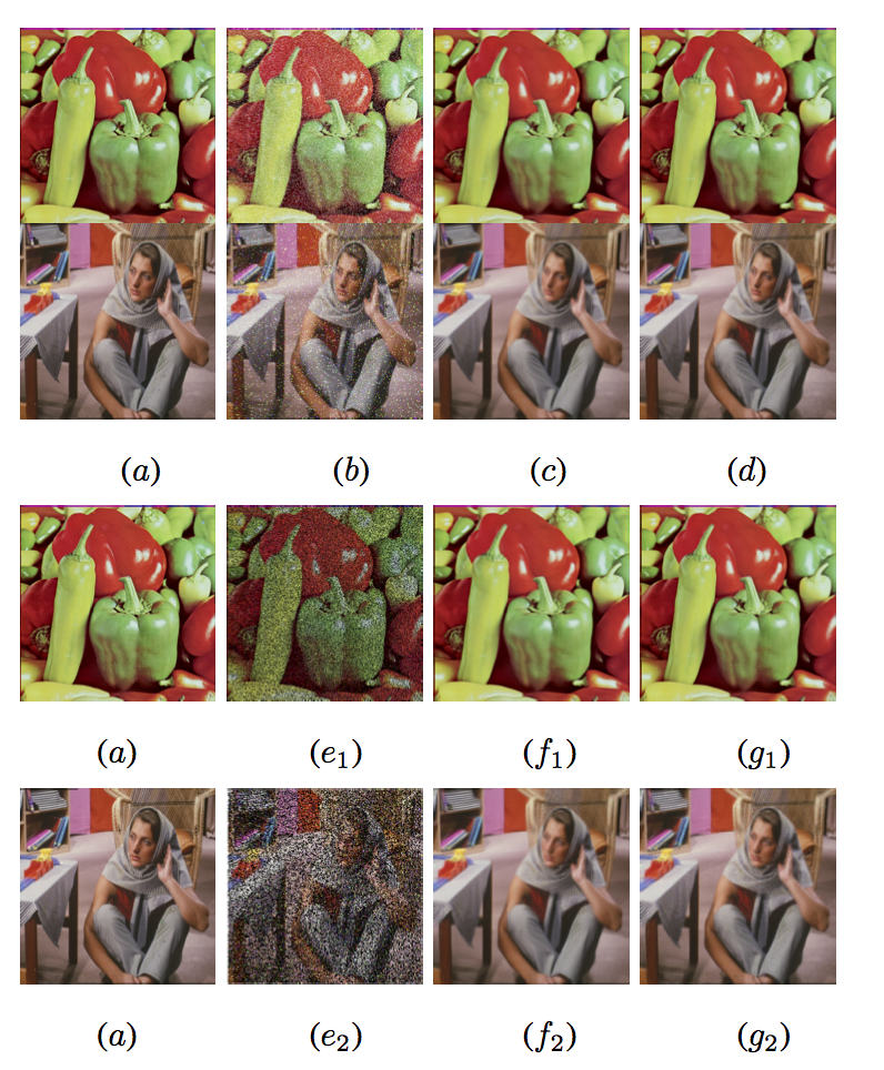
Figure 2: Inpainting results with different level:($a$) original, ($b$) ($1-\rho,\gamma$) = $(0,10\%)$, ($e_{1}$) ($1-\rho,\gamma$) = $(50\%,10\%)$, ($e_{2}$) ($1-\rho,\gamma$) = $(50\%,20\%)$, ($c$,$f_{1}$,$f_{2}$) NSS-QMC, ($d$,$g_{1}$,$g_{2}$) LRL-RQTC

.

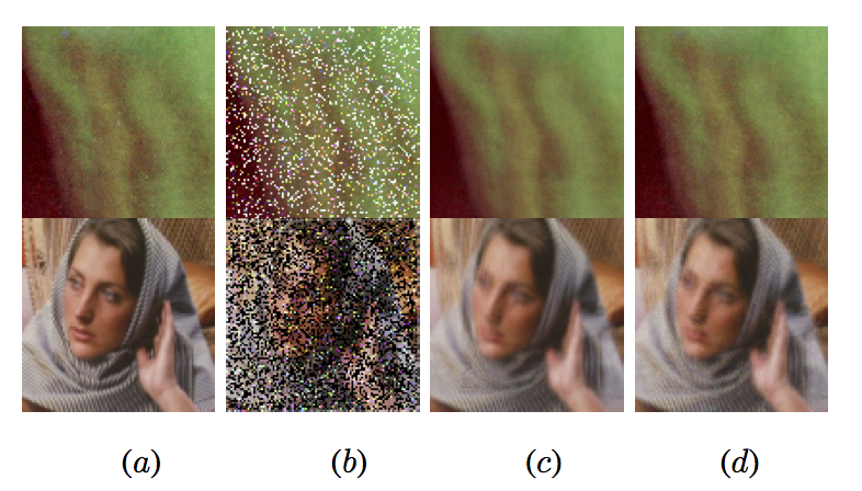
Figure 3: Enlarged parts of the first and forth row in Fig 2: (a) the original, (b) the observations, (c) NSS-QMC, (d) LRL-RQTC.

.

Example IV.2.

(Robust Color Video Recovery)

In this example, we compare the proposed RQTC and LRL-RQTC methods with other modern techniques in order to demonstrate the effectiveness and superiority of our methods in robust color video recovery. We choose the color video ‘DO01$\_$013’ in ‘videoSegmentationData’ database [3] of size $243\times 256$ and use a 3-mode quaternion tensor to represent it. We also compare the performance of models under different missing entries and noise levels.

We set $(1-\rho,\gamma)=(10\%,10\%),(20\%,10\%)$. The stopping criteria is $\delta=10^{-4}$ and suitable parameters are chosen to obtain the best results of each model. We compare RQTC and LRL-RQTC with the other six robust quaternion tensor completion methods.

• t-SVD (Fourier) [15]: Tensor SVD using Fourier transform.

• TNN [26]: Recover 3-D arrays with a low tubal-rank tensor.

• OITNN-O [21]: Recover tensors by new tensor norms: Overlapped Orientation Invariant Tubal.

• OITNN-L [21]: Recover tensors by new tensor norms: Latent Orientation Invariant Tubal Nuclear Norm.

• QMC [10]: Consider each frame of color video as a color image.

• TNSS-QMC [8]: Use distance function to find similar patches.

For t-SVD (Fourier), TNN, OITNN-O, OITNN-L, QMC, and TNSS-QMC, we strictly follow the parameters set in the article. For LRL-RQTC, we fix each window of size $27\times 32$ and only act on the frontal slice, i.e. $[\alpha_{1},\alpha_{2},\alpha_{3}]=[0,0,1]$. The maximum number of iterations is $100$, each patch size is $11\times 11$. For RQTC, the weighted vector $\alpha=[\alpha_{1},\alpha_{2},\alpha_{3}]=[0.8,0.1,0.1]$.

The detailed comparisons of the ‘DO01$\_$013’ dataset are given in Table II. We display the comparative results on ten frames randomly choosen from color video of two situations. From the last row of Table II, with respect to PSNR and SSIM, the suggested LRL-RQTC outperforms all other competitors on the average recovery results. Our LRL-RQTC exceeds the second-best by $0.7$ dB PSNR value on average. In particular, from the sub-table (a), the PSNR value of the restored frames of video can be increased by nearly 1dB under $10\%$ noise and missing entries level. From the sub-table (b), although on individual frames our LRL-RQTC is not as good as OITNN-L, the average result of our method is higher and the result of OITNN-L is not stable. Furthermore, different from patch-based methods such as TNSS-QMC and LRL-RQTC, our proposed RQTC recovers color video on the whole. Despite not reaching the highest PSNR and SSIM values, RQTC outperforms tsvd (Fourier), TNN, OITNN-O, and QMC which also processes the entire video without patching. It is worth noting that RQTC outperforms QMC by $3$ dB PSNR value and are only slightly less than the other patch’s method. The RQTC can also be handled very well in small details and the global approach is much faster than the patch-based approach, so we believe that there is much potential to improve RQTC.

In Fig. 4 and Fig. 5, we present the visual results on one frame under two conditions, where it can be seen that recovered video frames generated through the proposed RQTC and LRL-RQTC contain more details and more closely approximate the color of the initial frames. For instance, we observe the detailed features of the restored grass carefully. From the enlarged part (2nd row) of Fig. 4, color of shades and density of the grass in (c)th (h)th and (j)th columns have a clearer structure and look more realistic but the horse of (c)th column are not restored clearer. This means this video restored by our LRL-RQTC and RQTC are better. Although the PSNR and SSIM values of RQTC are not higher than TNSS-QMC, the recovery of certain details is superior to it. It shows that both RQTC and LRL-RQTC outperform in most cases. From the enlarged part (2nd row) of Fig. 5, the white point of the horse’s head is restored better by LRL-RQTC, it looks brighter and completer. The proposed LRL-RQTC uses the idea of clustering and finding similar patches adaptively by learning technology. Patches by learning technology can form low-rank matrices and make sure the effect of recovery is better. In particular, it is not necessary to calculate all singular values during the process. As a result, with the proper amount of patches, the suggested LRL-RQTC will be substantially more efficient.

TABLE II: PSNR AND SSIM VALUES BY DIFFERENT METHODS ON THE COLOR VIDEO.

(1) $(1-\rho,\gamma)=(10\%,10\%)$

Number of	t-SVD (Fourier)		TNN		OITNN-O		OITNN-L		QMC		RQTC		TNSS-QMC		LRL-RQTC
frames	PSNR	SSIM	PSNR	SSIM	PSNR	SSIM	PSNR	SSIM	PSNR	SSIM	PSNR	SSIM	PSNR	SSIM	PSNR	SSIM
1	32.76	0.9039	29.87	0.8938	30.33	0.8966	38.33	0.9764	33.51	0.9303	36.83	0.9525	38.79	0.9709	40.22	0.9785
2	31.71	0.8888	30.50	0.9105	33.95	0.9500	39.73	0.9799	33.63	0.9336	37.19	0.9544	39.56	0.9759	40.94	0.9814
3	32.08	0.8957	31.09	0.9245	35.59	0.9628	39.30	0.9780	33.84	0.9354	37.36	0.9553	40.09	0.9776	41.35	0.9823
4	32.57	0.8982	31.02	0.9254	35.99	0.9688	39.09	0.9793	33.83	0.9361	37.32	0.9560	39.75	0.9769	40.92	0.9810
5	32.59	0.9025	30.43	0.9167	35.64	0.9692	38.30	0.9778	33.86	0.9359	36.35	0.9524	39.32	0.9745	39.84	0.9771
6	32.64	0.9014	29.72	0.9045	35.22	0.9668	37.64	0.9763	33.76	0.9361	35.36	0.9495	37.59	0.9670	37.97	0.9716
7	31.60	0.8895	29.46	0.8899	34.58	0.9622	37.41	0.9765	33.85	0.9345	35.64	0.9527	38.32	0.9715	39.17	0.9749
8	32.32	0.8967	29.73	0.8907	33.72	0.9572	36.29	0.9732	34.16	0.9367	35.79	0.9539	39.15	0.9751	39.93	0.9778
9	32.54	0.8997	29.41	0.8870	32.75	0.9477	36.03	0.9725	34.09	0.9357	35.87	0.9535	39.40	0.9758	39.99	0.9783
10	32.58	0.9029	28.37	0.8679	28.56	0.8733	34.69	0.9683	34.18	0.9362	35.10	0.9506	38.61	0.9733	39.12	0.9757
average	32.34	0.8979	29.96	0.9011	33.63	0.9455	37.68	0.9758	33.8	0.9351	36.28	0.9531	39.06	0.9739	39.95	0.9778

(2) $(1-\rho,\gamma)=(20\%,10\%)$

Number of	t-SVD (Fourier)		TNN		OITNN-O		OITNN-L		QMC		RQTC		TNSS-QMC		LRL-RQTC
frames	PSNR	SSIM	PSNR	SSIM	PSNR	SSIM	PSNR	SSIM	PSNR	SSIM	PSNR	SSIM	PSNR	SSIM	PSNR	SSIM
1	31.96	0.8927	29.79	0.8920	30.32	0.8962	37.32	0.9662	32.94	0.9165	35.64	0.9369	37.77	0.9657	38.32	0.9698
2	31.13	0.8788	30.42	0.9091	33.97	0.9498	39.84	0.9801	32.99	0.9202	36.05	0.9400	38.75	0.9729	39.40	0.9761
3	31.41	0.8834	31.03	0.9237	35.63	0.9627	39.41	0.9881	33.10	0.9211	36.15	0.9406	39.05	0.9737	39.82	0.9776
4	31.98	0.8912	30.98	0.9249	36.00	0.9686	39.12	0.9794	32.95	0.9233	36.05	0.9415	38.31	0.9724	39.18	0.9759
5	31.99	0.8907	30.41	0.9166	35.65	0.9693	38.32	0.9780	32.83	0.9223	35.41	0.9388	37.09	0.9666	37.45	0.9692
6	31.97	0.8895	29.74	0.9052	35.25	0.9165	36.69	0.9666	33.00	0.9215	34.45	0.9393	37.12	0.9618	37.30	0.9655
7	31.04	0.8743	29.47	0.8901	34.57	0.9619	37.37	0.9663	32.99	0.9201	34.74	0.9425	37.71	0.9652	38.18	0.9681
8	31.53	0.8854	29.69	0.8901	33.68	0.9567	36.26	0.9630	33.08	0.9203	34.92	0.9431	38.24	0.9683	38.74	0.9707
9	31.82	0.8905	29.37	0.8861	32.72	0.9476	35.99	0.9622	32.82	0.9190	35.89	0.9429	38.50	0.9694	38.89	0.9715
10	32.15	0.8947	28.33	0.8672	28.54	0.8733	34.69	0.9586	32.86	0.9204	34.30	0.9401	37.79	0.9665	37.98	0.9680
average	31.70	0.8871	29.92	0.9005	33.62	0.9402	37.50	0.9708	32.96	0.9204	35.36	0.9406	38.03	0.9683	38.53	0.9712

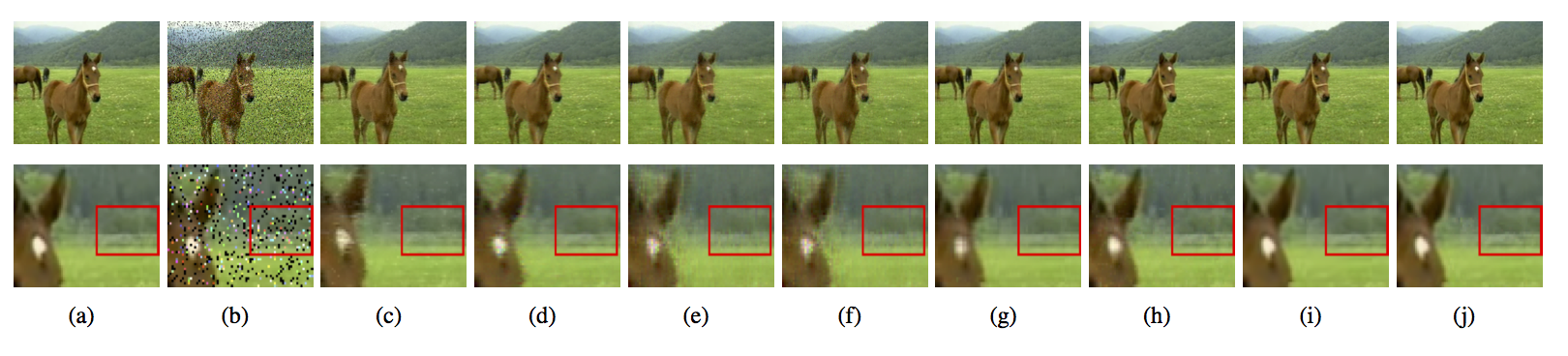
Figure 4: One frame (1st row) and their enlarged parts (2nd row) by eight methods with 10% unobserved and 10% corrupted entries. (a) the original. (b) the observations. (c) t-SVD (Fourier). (d) TNN. (e) OITNN-O. (f) OITNN-L. (g) QMC. (h) RQTC. (i) TNSS-QMC. (j) LRL-RQTC.

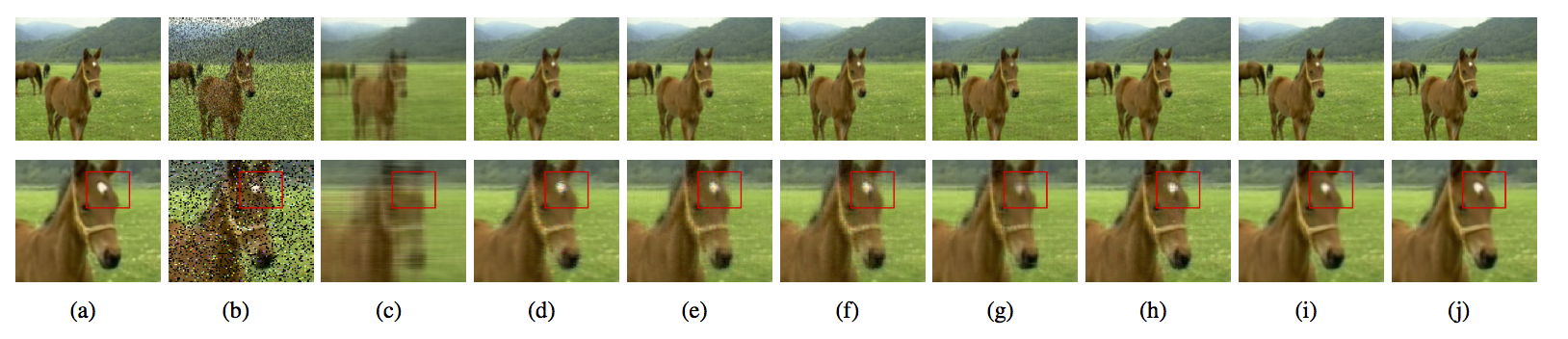
Figure 5: One frame (1st row) and their enlarged parts (2nd row) by eight methods with 20% unobserved and 10% corrupted entries. (a) the original images. (b) the observations. (c) t-SVD (Fourier). (d) TNN. (e) OITNN-O. (f) OITNN-L. (g) QMC. (h) RQTC. (i) TNSS-QMC. (j) LRL-RQTC.

Example IV.3.

(Color Video Completion)

In this example, we deal with the color video completion problem, which involves filling in missing pixel values from a partly unobserved video. Assume the missing pixels are distributed randomly across RGB three channels.

We compare the proposed RQTC and LRL-RQTC with representative models for color video completion: t-SVD (Fourier)[15], t-SVD (data)[19] (using a transform tensor singular value decomposition based on a unitary transform matrix), OITNN-O[21], OITNN-L[21], LRQTC[17] (quaternion tensor completion) , QMC[10] and TNSS-QMC[8].

The color video dataset is also chosen from the ‘videoSegmentationData’ database in [3]. We choose the color videos ‘BR130T’, ‘DO01$\_$030’, and ’DO01$\_$013’ of size $288\times 352$, which are denoted as ‘bird’, ‘flower’, and ‘horse’, respectively, and the videos can be expressed as 3-mode quaternion tensors. Their parameter values are empirically chosen to produce the greatest performance and are fixed in all testing for a fair comparison.

Different missing entries and noise levels are considered: $(1-\rho,\gamma)=(50\%,0\%),(80\%,0\%),(85\%,0\%)$. In the proposed LRL-RQTC, we fix each window of size $36\times 44$ and only act on the frontal slice, i.e.$[\alpha_{1},\alpha_{2},\alpha_{3}]=[0,0,1]$. The maximum number of iterations is $100$, each patch size is $8\times 8$. For RQTC, the weighted vector $\alpha=[\alpha_{1},\alpha_{2},\alpha_{3}]=[0.8,0.1,0.1]$.

For quantitative comparison, PSNR and SSIM values on the ‘bird’, ‘flower’, and ‘horse’ videos are reported in Fig. 6, Fig 9 and Table III. The corresponding visual examples are shown in Fig. 7 - 8, Fig. 10 - 11, and Fig. 12 - 13 for qualitative evaluation. In the four histograms (Fig. 6 and Fig 9), we can find that PSNR and SSIM in earthy yellow on the right-hand side are higher than the other. In Table III, we present the PSNR and SSIM values of random ten frames of the ’horse’ video to provide additional information. The standout performance is bolded and the underlined data indicates sub-optimal. It is clear that the proposed LRL-RQTC improves PSNR and SSIM values considerably. The PSNR values obtained by the LRL-RQTC on three color video data improve by almost $3$ dB when compared to the second-best method and are always at the highest value, demonstrating the proposed method’s superiority over the other good approaches presently in use. That implies our LRL-RQTC is the best among the ten methods and suitable for different types of video. In particular, the PSNR values achieved by the LRL-RQTC on the ’flower’ color video data increase by roughly $4$ dB when compared to the second-best method. As displayed in the graph, the proposed LRL-RQTC outperforms the rival method in terms of visual quality. It can be seen that our LRL-RQTC captures the detail of each frame properly, which implies that learning technology to find similar patches is superior. From Fig. 7, the videos restored by LRL-RQTC ($\ell$th column) are clearer and show more details of the bird’s wings as well as the foliage. Moreover, videos recovered by RQTC ($k$th column) also restores details of the original video. Both LRL-RQTC and RQTC are superior to the other methods in respect of local features’ recovery. In Fig. 10 - Fig. 13, the details of flower petals, grass, the tails of horse and so on recovered by LRL-RQTC are closer to the original frame. We present some of them and use the red box on the images for details.

For computing time, we display the result in Table IV. Because of TNSS-QMC and our LRL-RQTC are based on patch ideas, per-patch based operations can be paralleled, so we only show the average time of each window. From Table IV, we can observe that our LRL-RQTC gets better results without taking too long. It slightly less than OITNN-L which is also gets better recovery effect.

Remember that the LRL-RQTC model designed by using a learning perspective framework searches for similar structures adaptively and forms a low-rank structure based on the patch idea. This model is made feasible by the 2DQPCA-based classification function that characterizes the low-rank information from subspace structure after projection. Numerical results indicate that the LRL-RQTC model has clearly made a significant increase in its ability to find high-dimensional information in low-dimensional space and accurately identify the delicate correlations between the observed and unknown values.

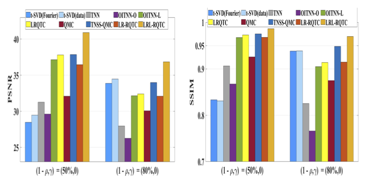
Figure 6: PSNR and SSIM comparisons on ‘bird’ color video.

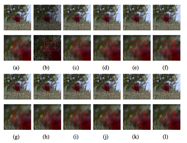
Figure 7: One frame (1st ans 3rd row) and their enlarged parts (2nd and 4th row) by ten methods with 50% unobserved entries. (a) the original. (b) the observations. (c) t-SVD (Fourier). (d) t-SVD (data). (e) TNN. (f) OITNN-O. (g) OITNN-L. (h) LRQTC. (i) QMC. (j) TNSS-QMC. (k) RQTC. ($\ell$) LRL-RQTC.

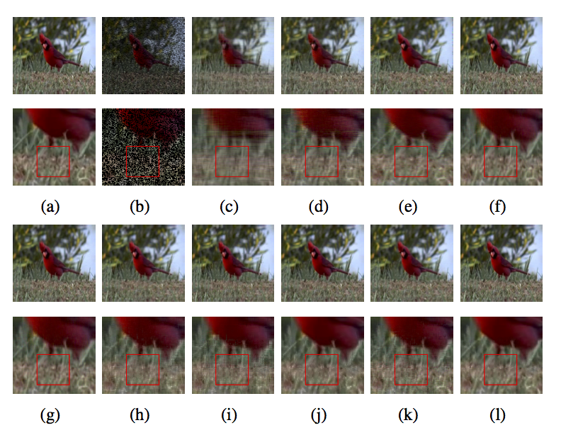
Figure 8: One frame (1st ans 3rd row) and their enlarged parts (2nd and 4th row) by ten methods with 85% unobserved entries. (a) the original. (b) the observations. (c) t-SVD (Fourier). (d) t-SVD (data). (e) TNN. (f) OITNN-O. (g) OITNN-L. (h) LRQTC. (i) QMC. (j) TNSS-QMC. (k) RQTC. ($\ell$) LRL-RQTC.

Figure 9: PSNR and SSIM comparisons on ‘flower’ color video.

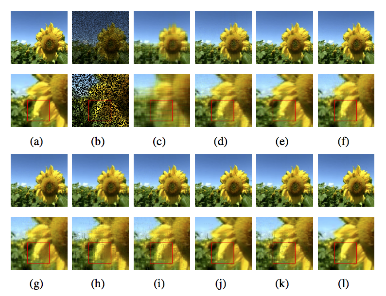
Figure 10: One frame (1st ans 3rd row) and their enlarged parts (2nd and 4th row) by ten methods with 80% unobserved entries. (a) the original. (b) the observations. (c) t-SVD (Fourier). (d) t-SVD (data). (e) TNN. (f) OITNN-O. (g) OITNN-L. (h) LRQTC. (i) QMC. (j) TNSS-QMC. (k) RQTC. ($\ell$) LRL-RQTC.

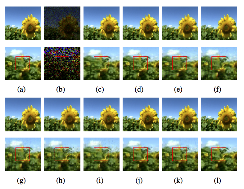
Figure 11: One frame (1st ans 3rd row) and their enlarged parts (2nd and 4th row) by ten methods with 85% unobserved entries. (a) the original. (b) the observations. (c) t-SVD (Fourier). (d) t-SVD (data). (e) TNN. (f) OITNN-O. (g) OITNN-L. (h) LRQTC. (i) QMC. (j) TNSS-QMC. (k) RQTC. ($\ell$) LRL-RQTC.

TABLE III: PSNR AND SSIM VALUES BY DIFFERENT METHODS ON “HORSE” COLOR VIDEO.

(1) $(1-\rho,\gamma)=(80\%,0)$

Number of	t-SVD (Fourier)		t-SVD (data)		TNN		OITNN-O		OITNN-L		LRQTC		QMC		TNSS-QMC		RQTC		LRL-RQTC
frames	PSNR	SSIM	PSNR	SSIM	PSNR	SSIM	PSNR	SSIM	PSNR	SSIM	PSNR	SSIM	PSNR	SSIM	PSNR	SSIM	PSNR	SSIM	PSNR	SSIM
1	29.29	0.8817	33.80	0.9435	33.74	0.9521	31.43	0.9016	31.38	0.9007	32.11	0.8815	29.77	0.8253	35.21	0.9408	33.02	0.8941	37.06	0.9599
2	28.47	0.8571	33.19	0.9339	34.72	0.9622	33.92	0.9369	33.89	0.9364	32.10	0.8843	29.71	0.8301	35.67	0.9453	33.18	0.8973	37.46	0.9629
3	28.89	0.8707	33.66	0.9405	35.39	0.9661	34.59	0.9440	34.56	0.9436	32.31	0.8851	30.09	0.8353	36.30	0.9505	33.36	0.9000	37.68	0.9637
4	29.54	0.8800	33.95	0.9412	34.99	0.9645	34.79	0.9485	34.75	0.9481	32.43	0.8886	30.13	0.8380	36.35	0.9504	33.39	0.8998	37.63	0.9644
5	29.58	0.8828	33.99	0.9429	34.18	0.9598	34.74	0.9505	34.71	0.9501	32.29	0.8873	30.04	0.8385	35.99	0.9489	33.20	0.8978	37.60	0.9647
6	29.29	0.8786	33.76	0.9409	33.58	0.9539	34.60	0.9484	34.56	0.9480	35.15	0.8795	30.11	0.8368	35.38	0.9413	32.56	0.8812	37.27	0.9621
7	28.30	0.8563	33.03	0.9341	33.12	0.9460	34.16	0.9451	34.12	0.9447	32.08	0.8784	30.04	0.8337	35.16	0.9373	32.59	0.8800	37.09	0.9593
8	28.56	0.8673	33.47	0.9400	33.04	0.9445	33.92	0.9433	33.89	0.9429	32.26	0.8798	30.04	0.8388	35.26	0.9375	32.69	0.8804	37.17	0.9595
9	29.13	0.8748	33.54	0.9396	33.02	0.9438	33.60	0.9360	33.56	0.9354	32.28	0.8800	30.02	0.8341	35.24	0.9374	32.70	0.8816	37.22	0.9595
10	28.94	0.8752	33.54	0.9426	31.74	0.9289	30.75	0.8940	30.71	0.8932	32.31	0.8808	30.08	0.8356	35.29	0.9389	32.67	0.8818	37.33	0.9601
average	29.04	0.8725	33.59	0.9299	33.75	0.9522	33.65	0.9348	33.61	0.9343	32.53	0.8808	30.00	0.8346	35.56	0.9428	32.94	0.8894	37.35	0.9616

(2) $(1-\rho,\gamma)=(85\%,0\%)$

Number of	t-SVD (Fourier)		t-SVD (data)		TNN		OITNN-O		OITNN-L		LRQTC		QMC		TNSS-QMC		RQTC		LRL-RQTC
frames	PSNR	SSIM	PSNR	SSIM	PSNR	SSIM	PSNR	SSIM	PSNR	SSIM	PSNR	SSIM	PSNR	SSIM	PSNR	SSIM	PSNR	SSIM	PSNR	SSIM
1	25.99	0.7562	30.42	0.8748	32.65	0.9373	30.28	0.8729	30.23	0.8718	31.66	0.8642	30.17	0.8737	33.94	0.9243	31.72	0.8560	37.16	0.9623
2	25.41	0.7251	29.93	0.8576	33.46	0.9486	32.51	0.9127	32.46	0.9118	31.63	0.8638	29.96	0.8317	33.65	0.9189	31.74	0.8544	36.93	0.9595
3	25.62	0.7418	30.19	0.8669	33.98	0.9548	33.07	0.9236	33.04	0.9230	31.72	0.8673	30.05	0.8334	33.50	0.9197	31.93	0.8568	37.02	0.9619
4	25.95	0.7524	30.45	0.8717	33.68	0.9536	33.27	0.9287	33.23	0.9280	31.67	0.8671	30.00	0.8333	33.44	0.9187	31.83	0.8556	37.03	0.9621
5	25.99	0.7572	30.54	0.8769	33.18	0.9490	33.28	0.9309	33.24	0.9302	31.56	0.8671	30.02	0.8372	33.29	0.9203	31.76	0.8557	36.84	0.9626
6	26.03	0.7568	30.55	0.8751	32.59	0.8414	33.24	0.9305	33.20	0.9300	31.65	0.8658	30.16	0.8375	33.31	0.9175	31.82	0.8585	37.21	0.9618
7	25.31	0.7285	29.75	0.8584	32.18	0.9335	32.87	0.9257	32.84	0.9251	31.64	0.8626	31.69	0.8555	33.45	0.9164	31.69	0.8555	36.95	0.9583
8	25.60	0.7402	30.28	0.8679	31.97	0.9280	32.68	0.9222	32.64	0.9216	31.97	0.8697	30.67	0.8406	34.05	0.9233	32.00	0.8616	37.27	0.9610
9	25.95	0.7552	30.52	0.8741	31.85	0.9261	32.35	0.9139	32.30	0.9129	31.97	0.8686	30.57	0.8411	34.14	0.9240	32.01	0.8608	37.51	0.9610
10	25.96	0.7552	30.55	0.8750	30.71	0.9094	29.68	0.8684	29.63	0.8673	31.86	0.8662	30.14	0.8360	34.19	0.9242	31.99	0.8601	37.35	0.9606
average	25.78	0.7468	30.32	0.8698	32.63	0.9383	32.32	0.9130	32.28	0.9122	31.73	0.8662	30.34	0.8420	33.70	0.9208	31.85	0.8575	37.13	0.9611

Figure 12: One frame (1st ans 3rd row) and their enlarged parts (2nd and 4th row) by ten methods with 80% unobserved entries. (a) the original. (b) the observations.(c) t-SVD (Fourier). (d) t-SVD (data). (e) TNN. (f) OITNN-O. (g) OITNN-L. (h) LRQTC. (i) QMC. (j) TNSS-QMC. (k) RQTC. ($\ell$) LRL-RQTC.

Figure 13: One frame (1st ans 3rd row) and their enlarged parts (2nd and 4th row) by ten methods with 85% unobserved entries. ((a) the original. (b) the observations. (c) t-SVD (Fourier). (d) t-SVD (data). (e) TNN. (f) OITNN-O. (g) OITNN-L. (h) LRQTC. (i) QMC. (j) TNSS-QMC. (k) RQTC. ($\ell$) LRL-RQTC.

TABLE IV: AVERAGE CPU TIME OF EACH FRAME OF THE RESTORED VIDEOS (UNIT:SECOND)

  Methods bird video flower video horse video (50%,0) (80%,0) (80%,0) (85%,0) (80%,0) (85%,0) t-SVD(Fourier) 8.22 9.64 6.61 6.87 6.67 6.83 t-SVD(data) 15.97 18.58 12.92 12.59 10.97 11.01 TNN 5.05 4.17 4.54 4.03 2.86 2.85 OITNN-O 36.25 35.57 36.41 18.30 24.08 12.50 OITNN-L 37.02 36.96 36.98 36.74 24.02 24.24 QMC 96.12 84.06 88.79 96.27 80.11 87.88 LRQTC 19.61 19.61 19.51 19.49 19.52 19.47 TNSS-QMC 15.31 16.05 14.75 14.78 13.29 12.18 RQTC 22.74 21.98 20.65 21.23 19.67 19.63 LRL-RQTC 26.21 24.62 25.25 26.92 23.84 22.98  

V Conclusion

In this article, we develop a new learning technology-based robust quaternion tensor completion model, LRL-RQTC. Firstly, we divide the observed large quaternion tensor into smaller quaternion sub-tensors and parallelly act on these quaternion sub-tensors. Secondly, we use 2DQPCA-based classification function to learning low-rank information of each slices and form them into a low-rank quaternion matrix. Then RQTC problem of each quaternion sub-tensors can be solved. The recommended technique focuses on keeping as many low-rank correlations among the local characteristics of color videos as feasible in order to preserve more related information under the framework. A new RQTC model is also proposed to solve RQTC problem by ADMM-based framework. We establish conditions for quaternion tensor incoherence and exact recovery theory. Numerical experiments on the established RQTC and LRL-RQTC models demonstrate that our proposed models can inpaint a given missing and/or corrupted quaternion tensor better, maintaining a low-rank structure for processing nature color videos both effectively and efficiently. In order to make the most of the information between images and get a faster and more efficient algorithm, we will strive to develop a learning technology combined with other advanced technology for quaternion tensor decomposition in the future.

References

- [1] S. Boyd, N. Parikh, E. Chu, B. Peleato, and J. Eckstein, “Distributed optimization and statistical learning via the alternating direction method of multipliers”, Foundations and Trends® in Machine Learning, 3 (2011), pp. 1–122.
- [2] J. Chen and M. Ng, “Color Image Inpainting via Robust Pure Quaternion Matrix Completion: Error Bound and Weighted Loss”, SIAM Journal on Imaging Sciences 15, 3 (2022), pp. 1469–1498.
- [3] K. Fukuchi, K. Miyazato, A. Kimura, S. Takagi, and J. Yamato, “Saliency-based video segmentation with graph cuts and sequentially updated priors”, IEEE International Conference on Multimedia and Expo (2009), pp. 638–641.
- [4] K. Gao and Z. Huang, “Tensor Robust Principal Component Analysis via Tensor Fibered Rank and Minimization”, SIAM Journal on Imaging Sciences, vol. 16, no. 1 (2023), pp. 423–460.
- [5] W. R. Hamilton, “Elements of Quaternion”, Longmans, Green and Co., London (1866).
- [6] B. Huang, C. Mu, D. Goldfarb, and J. Wright, “Provable low-rank tensor recovery”, Optim.-Online, vol. 4252, no. 2, (2014), Art. no. 4252.
- [7] H. Huang, Y. Liu, Z. Long and C. Zhu, “Robust Low-Rank Tensor Ring Completion”, IEEE Transactions on Big Data, (2023), pp. 1–14.
- [8] Z. Jia, Q. Jin, M. Ng, and X. Zhao, “Non-local robust quaternion matrix completion for large-scale color image and video Inpainting”, IEEE Transactions on Image Processing, 31 (2022), pp. 3868-3883.
- [9] Z. Jia, S. Ling, and M. Zhao, “Color two-dimensional principal component analysis for face recognitionbased on quaternion model”, Lecture Notes in Computer Science, 10361 (2017), pp. 177-189.
- [10] Z. Jia, M. Ng, and G. Song, “Robust quaternion matrix completion with applications to image inpainting”, Numerical Linear Algebra with Applications, 26(4) (2019), pp. e2245.
- [11] T. Jiang, X. Zhao, H. Zhang and M. Ng, “Dictionary Learning With Low-Rank Coding Coefficients for Tensor Completion”, IEEE Transactions on Neural Networks and Learning Systems, vol. 34, no. 2 (2023), pp. 932-946.
- [12] T. Kolda, and B. Bader, “Tensor decompositions and applications”, SIAM Review, 51, 3 (2009), pp. 455–500.
- [13] Y. Li, D. Qiu, and X. Zhang, “Robust Low Transformed Multi-Rank Tensor Completion With Deep Prior Regularization for Multi-Dimensional Image Recovery”, IEEE Transactions on Big Data, (2023), pp. 1–14.
- [14] J. Liu, P. Musialski, P. Wonka, and J. Ye, “Tensor completion for estimating missing values in visual data”, ICCV (2009), pp. 2114–2121.
- [15] C. Lu, J. Feng, Y. Chen, W. Liu, Z. Lin, and S. Yan, “Tensor robust principal component analysis with a new tensor nuclear norm”, IEEE Transactions on Pattern Analysis and Machine Intelligence, vol. 42, no. 4 (2020), pp. 925–938.
- [16] Y. Luo, X. Zhao, T. Jiang, Y. Chang, M. Ng and C. Li, “Self-Supervised Nonlinear Transform-Based Tensor Nuclear Norm for Multi-Dimensional Image Recovery”, IEEE Transactions on Image Processing, vol. 31 (2022), pp. 3793-3808.
- [17] J. Miao, K. I. Kou, and W. Liu, “Low-rank quaternion tensor completion for recovering color videos and images”, Pattern Recognition, vol. 107 (2020), Art. no. 107505.
- [18] M. Ng, X. Zhang, X. Zhao, “Patched-tube unitary transform for robust tensor completion”, Pattern Recognition, vol. 100 (2020), Art. no. 107181..
- [19] G. Song, M. Ng, and X. Zhang, “Robust tensor completion using transformed tensor singular value decomposition”, Numerical Linear Algebra with Applications, 27 (3) (2020), e2299.
- [20] L. Tucker, “Some mathematical notes on three-mode factor analysis”, Psychometrika, 31, 3 (1966), pp. 279–311.
- [21] A. Wang, Q. Zhao, Z. Jin, et al., “Robust tensor decomposition via orientation invariant tubal nuclear norms”, Science China Technological Sciences 65 (2022), pp. 1300–1317 .
- [22] Z. Wang, A. Bovik, H. Sheikh and E. Simoncelli, “Image quality assessment: from error visibility to structural similarity”, IEEE Transactions on Image Processing vol. 13, no. 4 (2004), pp. 600–612.
- [23] T. Xu, X. Kong, Q. Shen, Y. Chen, and Y. Zhou, “Deep and Low-Rank Quaternion Priors for Color Image Processing”, IEEE Transactions on Circuits and Systems for Video Technology (2022), doi: 10.1109/TCSVT.2022.3233589.
- [24] J. Yang, D. Zhang, A. Frangi, and J. Yang, “Two-dimensional PCA: A new approach to appearance-based face representation and recognition”, IEEE Transactions on Pattern Analysis and Machine Intelligence, vol. 26, no. 1 (2004), pp. 131-137.
- [25] F. Zhang, “Quaternions and matrices of quaternions”, Linear Algebra and its Applications, 251 (1997), pp. 21–57.
- [26] Z. Zhang and S. Aeron, “Exact Tensor Completion Using t-SVD”, IEEE Transactions on Signal Processing, vol. 65, no. 6 (2017), pp. 1511-1526.
- [27] X. Zhao, M. Bai, D. Sun, and L. Zheng, “Robust Tensor Completion: Equivalent Surrogates, Error Bounds, and Algorithms”, SIAM Journal on Imaging Sciences, vol. 15, no. 2 (2022), pp. 625–669.