Properties of Villarceau Torus

Abstract

This is an initial draft of ongoing research. This incomplete research is submitted to Kuwait University for research funding. The project proposal is under processing. Please do not hesitate to write your comments to improve the quality of the paper. You will reach me at the email address stated above. I will be pleased to interact with you.

Keywords: Villarceau torus; isometric and convex cycle; toroidal helices, Network distance; congestion-balanced routing;

AMS Subj. Class.: 05C12, 05C70, 68Q17

1 Introduction

One interesting geometrical problem related to celestial surfaces posed by 19th century mathematicians was ”Given an arbitrary point P on a surface, how many distinct circles can be drawn on the surface passing through the point P?”. This was called the n-circle property. While a sphere has the infinite circle property, it was shown that some surfaces have the n-circle property for n equal to 4, 5 or 6 [1]. A startling conjecture by Richard Blum [1] is that there are no surfaces with the n-circle property for n greater than 6 and less than infinity. A surface which was attracted by 19th century mathematicians was torus. Until 1848, torus was known only by two circles which are toroidal and poloidal circles. In 1848, Yvon Villarceau demonstrated two diagonal circles on a torus [23, 24]. The toroidal circle of a torus is horizontal and lies in the plane of the torus. The poloidal circle is vertical and is perpendicular to the toroidal. The third and fourth circles are obliquely inclined with respect to the first two circles of the torus and are known as the Villarceau circles [23]. Refer to Figure 1. In other words, Villarceau circles are a pair of circles produced by cutting a torus obliquely through the center at a special angle $\theta$ [23]. At the given point P on the torus, while the third circle makes an acute angle with the horizontal plane, the fourth one makes an obtuse angle with horizontal plane [23]. Following Villarceau circles, there were two types of tori. A torus built by toroidal and poloidal circles is called grid (ring) torus and a torus built by the Villarceau circles is called Villarceau torus. Refer to Figure 2. In Physics, it is called spiral torus [8, 10]. The $2$-dimensional representation of Villarceau torus is shown in Figure 3.

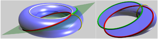
Figure 1: The toroidal circle (white color) of a torus is horizontal and lies in the plane of the torus. The poloidal circle (yellow color) is vertical and is perpendicular to the toroidal. The third and fourth circles (red and green colors) are obliquely inclined with respect to the first two circles of the torus and are known as the Villarceau circles. The diagrams are retrieved from [23].

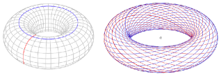
Figure 2: Ring torus and Villarceau torus. The diagrams are extracted from Wikimedia Commons.

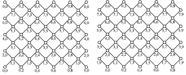
Figure 3: The 2D representation of Villarceau torus ${\rm VT}(4,5)$. One is a cyclic rotation of the other.

2 Terminologies and some observations of Villarceau torus ${\rm VT}(r,s)$

In Discrete Mathematics, $(Z_{n},\oplus_{n})$ represents the additive group of integers modulo $n$ where $Z_{n}=\{0,1\ldots n-1\}$ and $a\oplus_{n}b=(a+b)\mod n$. The $2$-dimensional representation of Villarceau torus which are the projection of $3$-dimensional torus onto a $2$-dimensional plane was studied by several authors [2, 7, 20]. Refer to Figure 3. The Villarceau torus is denoted by ${\rm VT}(rs)$ where the addition in both coordinates is modular addition. The addition of two vertices $(r_{1},s_{1})$ and $(r_{2},s_{2})$ in ${\rm VT}(r,s)$ is defined as follows:

$$(r_{1},s_{1})+(r_{2},s_{2})=(r_{1}+r_{2},s_{1}+s_{2})=(r_{1}\oplus_{2r}r_{2},s_{1}\oplus_{2s}s_{2})$$

The vertex set $V$ of ${\rm VT}(r,s)$ is $V$ = $\{(2i+1,2j+1):0\leq i\leq r-1,0\leq j\leq s-1\}\cup\{(2i,2j):0\leq i\leq r-1,0\leq j\leq s-1\}$. The edge set $E$ of ${\rm VT}(r,s)$ is $E=\{(2i,2j)(2i+1,2j+1),(2i,2j)(2i+1,2j-1):0\leq i\leq r-1,0\leq j\leq s-1\}$. See Figure 3.

A subgraph $H$ in $G$ is isometric, if $d_{H}(u,v)=d_{G}(u,v)$ for every pair $u$ and $v$ of vertices of $H$. A set S of vertices in $G(V,E)$ is convex if for each pair $x$ and $y$ of vertices in $S$, each isometric $x,y$-path entirely lies inside $S$. A cycle or path is isometric (resp. convex) if its induced subgraph is isometric (resp. convex). Here are some facts on convex paths and cycles which we recall to refresh our knowledge. A convex cycle (resp. path) is an isometric cycle (resp. path). Even cycles are not convex but odd cycles are convex. In an even cycle, a diametral path is not convex. However, in an odd cycle, every path is convex. Now we list some terminologies and notations which we use frequently in this paper.

While a path and a cycle are denoted by $P$ and $C$ respectively, an isometric path and an isometric cycle are denoted by $IP$ and $IC$ respectively. The edges in $VT(r,s)$ are either acute or obtuse [6, 7, 20]. See Figure 3. The set of acute edges of ${\rm VT}(r,s)$ is denoted by $E_{a}$ and the set of obtuse edges of ${\rm VT}(r,s)$ is denoted by $E_{o}$. In other words, the edge set $E$ of ${\rm VT}(r,s)$ is partitioned by acute edges and obtuse edges such that $E=E_{a}\cup E_{o}$, $E_{a}\cap E_{o}=\emptyset$, and $|E_{a}|=|E_{o}|$. A path in ${\rm VT}(r,s)$ is called an acute (resp. obtuse) path if it contains only acute (resp. obtuse) edges. In the same way, a cycle in ${\rm VT}(r,s)$ is called an acute (resp. obtuse) cycle if it contains only acute (resp. obtuse) edges. An acute (resp. obtuse) path is represented by ${\rm AP}$ (resp. ${\rm OP}$). In the same way, an acute (resp. obtuse) cycle is represented by ${\rm AC}$ (resp. ${\rm OC}$).

Now, we define acute and obtuse paths of ${\rm VT}(r,s)$ as follows:

${\rm AP}(0,2k)=(0,2k)(1,2k+1)\ldots(i,2k+i)\ldots(2r-1,2k+(2r-1))(0,2k+2r)$, for $k=0,1\ldots s-1$.

${\rm OP}(0,2k)=(0,2k)(1,2k-1)\ldots(i,2k-i)\ldots(2r-1,2k-(2r-1))(0,2k-2r)$, for $k=0,1\ldots s-1$.

The path ${\rm AP}(0,2k)$ consists of only acute edges and it is an acute path. Similarly, ${\rm OP}(0,2k)$ is an obtuse path. Now, we define acute cycle ${\rm AC}(0,2k)$ and obtuse cycle ${\rm OC}(0,2k)$ of ${\rm VT}(r,s)$. Cycle ${\rm AC}(0,2k)$ extends ${\rm AP}(0,2k)$ along the acute edges until it reaches $(0,2k)$ as follows:

${\rm AC}(0,2k)=(0,2k)(1,2k+1)\ldots(i,2k+i)\ldots(2r-1,2k+(2r-1))(0,2k+2r)\ldots(2r-1,2k-1)(0,2k)$, for $k=0,1\ldots s-1$.

The above definition is well-defined because vertex $(0,2k)$ has only two acute edges $(0,2k)(1,2k+1)$ and $(2r-1,2k-1)(0,2k)$. If a cycle exits at $(0,2k)$ through $(0,2k)(1,2k+1)$, then it will reach back to $(0,2k)$ only through $(2r-1,2k-1)(0,2k)$. Moreover, The cycle ${\rm AC}(0,2k)$ consists of only acute edges and thus it is an acute cycle.

In the same way, ${\rm OC}(0,2k)$ extends the obtuse path ${\rm OP}(0,2k)$ along the obtuse edges until it reaches $(0,2k)$:

${\rm OC}(0,2k)=(0,2k)(1,2k-1)\ldots(i,2k-i)\ldots(2r-1,2k-(2r-1))(0,2k-2r)\ldots(2r-1,2k+1)(0,2k)$, for $k=0,1\ldots s-1$.

A graph $G$ is said to be uniform geodesic if all the maximal isometric paths of $G$ are of uniform length ${\rm diam}(G)$. The striking difference between ring torus $C_{r}\,\square\,C_{s}$ and Villarceau torus ${\rm VT}(r,s)$ are the results given below:

Property 2.1.

Let ${\rm VT}(r,s)$ denote a Villarceau torus.

1. While the diameter of $C_{r}\,\square\,C_{s}$ is $r+s$, the diameter of ${\rm VT}(r,s)$ is $\max\{r,s\}$.

2. While ring torus is uniform geodesic, Villarceau torus is not uniform geodesic. Villarceau torus ${\rm VT}(r,s)$ has maximal isometric paths of length $r$ as well as maximal isometric paths of length $s$.

We shall use the following facts at a later stage:

Property 2.2.

Let ${\rm VT}(r,s)$ denote a Villarceau torus where $s$ is assumed to be larger than $r$.

1. The vertex set $V$ and the acute edge set $E_{a}$ of $VT(r,s)$ are partitioned by paths $\{{\rm AP}(0,2k):k=0,\ldots,s-1\}$. In the same way, the vertex set $V$ and the obtuse edge set $E_{o}$ of ${\rm VT}(r,s)$ is partitioned by paths $\{{\rm OP}(0,2k):k=0,\ldots,s-1\}$.

2. The cycles ${\rm AC}(x,y)$ $($resp. ${\rm OC}(x,y))$ are unique because they are restricted to running through only acute (resp. obtuse) edges. In other words, given a vertex $(x,y)$ in ${\rm VT}(r,s)$, there exists only one acute cycle ${\rm AC}(x,y)$ and only one obtuse cycle ${\rm OC}(x,y)$ passing through $(x,y)$.

3 Toroidal helices in ${\rm VT}(r,s)$

A toroidal helix is a coil wrapped around a torus. It revolves around the poloidal direction as well as toroidal direction and is characterized by the number of revolutions it winds around the torus [27, 28]. Moreover, the wrapping angle of a toroidal helix against all the toroidal and poloidal cycles of the torus is a constant angle $\theta$ [21, 27]. In this section, we study the mathematical properties of the toroidal helical motion in the magnetic field by means of Villarceau torus. Refer to Figure 4. behind Since a toroidal helix flows around poloidal and toroidal direction, there are two types of revolutions [27]:

1. Poloidal Revolution which spirals around the poloidal direction.

2. Toroidal Revolution which spirals around the toroidal direction.

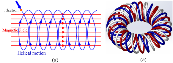
Figure 4: $(a)$ The diagram is extracted from https://www.schoolphysics.co.uk $(b)$ Toroidal helices in ${\rm VT}(r,s)$. The diagram is extracted from https://grabcad.com/library/toroidal-helix-1.

Here is a basic result in number theory which is available in most textbooks on number theory.

Theorem 3.1.

[11] Given two integers $a$ and $b$ such that $b$ is larger than $a$, let $d=\gcd(a,b)$, $p=a/d$ and $q=b/d$. Then $V=\{0,1,\ldots,b-1\}$ is partitioned into $V_{0},V_{1}\cdots,V_{d-1}$ where $V_{0}=\{0,a\cdots(q-1)\cdot a\}$, $V_{1}=\{1,1+a\cdots 1+(q-1)\cdot a\}$ $\cdots$, $V_{d-1}=\{(d-1),(d-1)+a,\cdots(d-1)+(q-1)\cdot a\}$.

The above result is applied in the following two theorems.

Theorem 3.2.

[19] Given two integers $a$ and $b$, let $d$ = $\gcd(a,b)$. Let $C_{b}(a)$ denote a circulant graph where its vertex set $V=\{0,1,\ldots b-1\}$. Then there exists a partition $\{S_{1},\cdots,S_{d}\}$ of $V$ such that the following statements are true:

1. The induced subgraphs $G[S_{1}],\cdots,G[S_{d}]$ are mutually disconnected components.

2. Each $G[S_{i}]$, $i=1,\ldots,d$ induces an isometric cycle of equal length in $C_{b}(a)$.

In other words, the vertex set $V$ as well as the edge set $E$ of $C_{b}(a)$ are partitioned by isometric cycles $C_{1},\cdots,C_{d}$ of equal length.

Theorem 3.1 is used as a tool to prove Theorem 3.2. In the same way, Theorem 3.2 will be used as a tool to prove Theorem 3.3.

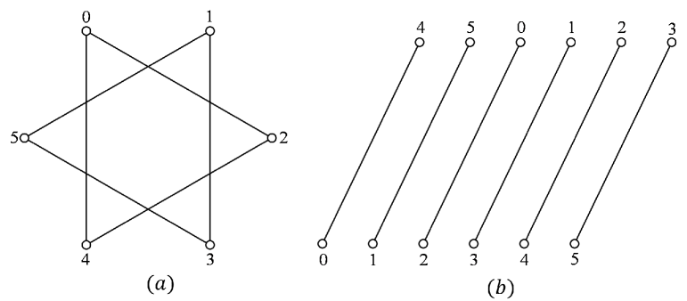
Figure 5: $(a)$ Circulant graph $C_{6}(4)$. $(b)$ The edges of $C_{6}(4)$ are arranged in a linear order.

Theorem 3.3.

Let $d=\gcd(r,s)$ of ${\rm VT}(r,s)$ where $s$ is larger than $r$. Then,

1. Exactly $d$ members of $\{{\rm AC}(0,2k):k=0,1\ldots s-1\}$ are distinct.

2. The vertex set $V$ of ${\rm VT}(r,s)$ is partitioned by those $d$ distinct members of $\{{\rm AC}(0,2k):k=0,1\ldots s-1\}$.

3. The acute edge set $E_{a}$ of ${\rm VT}(r,s)$ is partitioned by those $d$ distinct members of $\{{\rm AC}(0,2k):k=0,1\ldots s-1\}$.

Similar results are true for obtuse cycles ${\rm OC}(0,2k)$ and obtuse edge set $E_{o}$.

Proof.

Since each path ${\rm AP}(0,2k)$ contains only acute edges, any two members of $\{{\rm AP}(0,2k):k=0,1\ldots s-1\}$ are either mutually disjoint or isomorphic. By Property 2.2, the vertex set $V$ and acute edge set $E_{a}$ of ${\rm VT}(r,s)$ are partitioned by paths {${\rm AP}(0,2k):k=0,1$, $\ldots$, $s-1$}. The graph $C_{b}(a)$ and its edges are displayed in Figure 5. we will show that the acute paths $\{{\rm AP}(0,2k):k=0,\ldots,s-1\}$ are equivalent to the edges of $C_{b}(a)$. This is achieved by means of the following steps:

Step 1:

First, all the obtuse edges are removed from ${\rm VT}(r,s)$. Refer to Figure 6.

Step 2:

Path ${\rm AP}(0,2k)$ is replaced by edge $(0,2k)(0,2k+2r)$ for $k=0,\ldots,s-1$ where $(0,2k)$ and $(0,2k+2r)$ are the endpoints of ${\rm AP}(0,2k)$. This is achieved in two stages which are illustrated in Figure 7.

Step 3:

Label $(0,2k)$ are replaced by label $k$ for $k=0,\ldots,s-1$. Refer to Figure 8.

Step 4:

The resultant graph is isomorphic to $C_{6}(4)$ which is displayed in Figure 5.

Now the theorem follows from Theorem 3.2. ∎

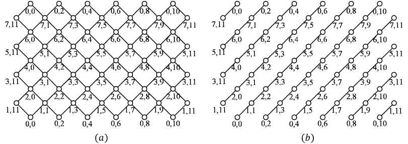
Figure 6: $(a)$ Villarceau torus ${\rm VT}(4,6)$. $(b)$ The obtuse edges are removed from ${\rm VT}(4,6)$.

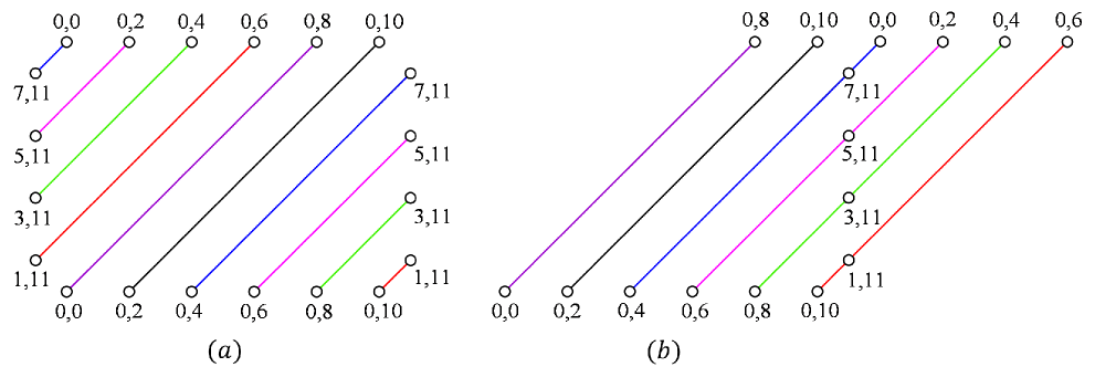
Figure 7: $(a)$ After removing obtuse edges from ${\rm VT}(r,s)$, In ${\rm VT}(r,s)$, the end vertices $(0,2k)$ and $(0,2k+2r)$ of ${\rm AP}(0,2k)$ are replace an edge $(0,2k)(0,2k+2r)$. Some lines between $(0,2k)$ and $(0,2k+2r)$ are broken into two segments which are distinguished by different colors. $(b)$ The broken segments are merged into one straight line.

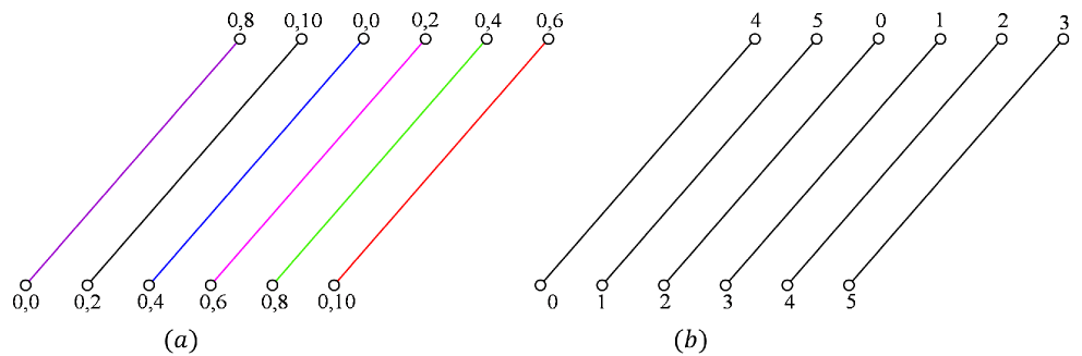
Figure 8: $(a)$ Now the acute path ${\rm AP}(0,2k)$ is replaced by an edge. $(b)$ The label $(0,2k)$ is replaced by $k$ for $k=0,\ldots,s-1$. This is isomorphic to $C_{6}(4)$ which is described in 5$(b)$.

Now we define a few more terms which we shall use in this section. First we define row and columns of ${\rm VT}(r,s)$:

$ROW_{2i}=\{(2i,0),(2i,2)\ldots(2i,2k)\ldots(2i,2(s-1)):i=0,1\ldots r-1\}$

$ROW_{(2i+1)}=\{(2i+1,1),(2i+1,3)\ldots(2i+1,2k+1)\ldots(2i+1,2s-1):i=0,1\ldots r-1\}$

$COL_{2j}=\{(0,2j),(2,2j)\ldots(2k,2j)\ldots(2(r-1),2j):j=0,1\ldots s-1\}$

$COL_{(2j+1)}=\{(1,2j+1),(3,2j+1)\ldots(2k+1,2j+1)\ldots(2r-1,2j+1):j=0,1\ldots s-1\}$

Given $ROW_{i}$ and $COL_{j}$, a cycle $C$ in ${\rm VT}(r,s)$ is said to have $p$ poloidal revolutions and $q$ toroidal revolutions if $C$ passes through $ROW_{i}$ by $p$ times and passes through $COL_{j}$ by $q$ times. Mathematically, given $ROW_{i}$ and $COL_{j}$, a cycle $C$ is said to have $p$ poloidal revolutions and $q$ toroidal revolutions if $|C\cap ROW_{i}|=p$ and $|C\cap COL_{j}|=q$.

Theorem 3.4.

Given ${\rm VT}(r,s)$, let $d=\gcd(r,s)$, $p=r/d$ and $q=s/d$ where $s$ is assumed to be larger than $r$. Then, cycle ${\rm AC}(0,2k)$ has $p$ toroidal revolutions and $q$ poloidal revolutions.

Proof.

Consider two columns $COL_{j_{1}}$ and $COL_{j_{2}}$ such that $j_{1}\neq j_{2}$. Since ${\rm AC}(0,2k)$ contains only acute edges, $|{\rm AC}(0,2k)\cap COL_{j_{1}}|=|{\rm AC}(0,2k)\cap COL_{j_{2}}|$. Here, ${\rm AC}(0,2k)\cap COL_{j_{1}}$ is the set of vertices common to both ${\rm AC}(0,2k)$ and $COL_{j_{1}}$. By Theorem 3.3, we know that $|{\rm AC}(0,2k_{1})|=|{\rm AC}(0,2k_{2})|$ for $k_{1}\neq k_{2}$. Also, by Theorem 3.3, the number of distinct cycles in $\{{\rm AC}(0,2k):k=0,1\ldots s-1\}$ is $d$. Since $COL_{j}$ has $r$ vertices and there are $d$ distinct cycles in $\{{\rm AC}(0,2k):k=0,1\ldots s-1\}$, each cycle ${\rm AC}(0,2k)$ shares exactly $r/d$ vertices with $COL_{j}$. It means that ${\rm AC}(0,2k)$ has $p$ toroidal revolutions. Similarly, ${\rm AC}(0,2k)$ has $q$ poloidal revolutions. ∎

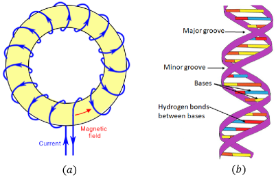
Figure 9: $(a)$ Toroidal Magnetic Field. The diagram is retrieved from https://www.sciencefacts.net/toroid-magnetic-field.html $(b)$ Double stranded helix model of DNA. This diagram is retrieved from https://www.vedantu.com/.

The Heat Transfer in Laminar Flows is modeled by means of toroidal helix [28]. The models of the electron illustrate that electrons internally move around a torus [12]. The electrons move on helix trajectories in a uniform magnetic field. It is called Helical Toroidal Electron Model [5, 28]. Refer to Figure 9 $(a)$. 3.4 provides the mathematical interpretation of the Helical Toroidal Electron Model.

Molecular biologists have modeled DNA strands in terms toroidal helices and call it as double stranded helix model of DNA. A DNA molecule consists of two strands that twist around one another to form a helix. Refer to Figure 9 $(b)$. This twisted-ladder structure double helix (DNA) was discovered by James Watson and Francis Crick in 1953 [25]. The double helix structure of DNA contains a major groove and minor groove which are similar to acute and obtuse cycles in ${\rm VT}(r,s)$ [13].

The toroidal helix in Physics and Molecular Biology is continuous whereas the toroidal helix in Villarceau torus is discrete.

4 Isometric and convex cycles in ${\rm VT}(r,s)$

Theorem 4.1.

Cycles ${\rm AC}(0,2k)$ and ${\rm OC}(0,2k)$, $k=0,\ldots,r-1$, are isometric but not convex in ${\rm VT}(r,r)$.

Proof.

In the square Villarceau torus ${\rm VT}(r,r)$, the end vertices of path ${\rm AP}(0,2k)$ are $(0,2k)$ and $(0,2k+2r)=(0,2k)$. Since the end vertices of path ${\rm AP}(0,2k)$ are the same, it becomes a cycle and isometric. Notice that this is not true for ${\rm VT}(r,s)$ where $r\neq s$.

Consider cycles ${\rm AC}(0,0)$ and ${\rm OC}(0,0)$. They do not have any edges in common. Moreover, ${\rm AC}(0,0)$ and ${\rm OC}(0,0)$ are of same size and meet only at two vertices $(0,0)$ and $(r,r)$ which are diagonally opposite. In other words, the cycles ${\rm AC}(0,0)$ and ${\rm OC}(0,0)$ are orthogonal as in Figure 10. Thus, cycles ${\rm AC}(0,0)$ and ${\rm OC}(0,0)$ are not convex. Since ${\rm VT}(r,r)$ is symmetric, we can extend the arguments to show that ${\rm AC}(0,2k)$ and ${\rm OC}(0,2k)$, $k=0,1\ldots s-1$, are not convex. ∎

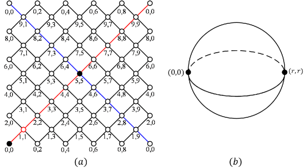
Figure 10: $(a)$ Cycles ${\rm AC}(0,0)$ is marked in red and ${\rm OC}(0,0)$ is marked in blue. $(b)$The two cycles intersect only at vertices $(0,0)$ and $(r,r)$ which are diametrically opposite. Since $|{\rm AC}(0,0)|=|{\rm OC}(0,0)|$, ${\rm AC}(0,0)$ and ${\rm OC}(0,0)$ are not convex cycles.

We leave a remark that Theorem 4.1 is true for ${\rm VT}(r,s)$ where $s$ is a multiple of $r$. The next result is interesting that Cycles ${\rm AC}(0,2k)$ and ${\rm OC}(0,2k)$ are not isometric in ${\rm VT}(r,s)$, when $s$ is not a multiple of $r$.

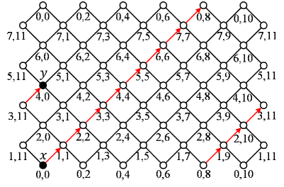
Figure 11: Here $x=(2r_{1},0)$ and $y=(2r_{2},0)$. The distance between $x$ and $y$ along $COL_{0}$ is strictly less than the distance between $x$ and $y$ along ${\rm AC}(0,2k)$.

Theorem 4.2.

Cycles ${\rm AC}(0,2k)$ and ${\rm OC}(0,2k)$, $k=0,\ldots,r-1$, are not isometric in ${\rm VT}(r,s)$, when $s$ is not a multiple of $r$.

Proof.

Let $d=\gcd(r,s)$. By Theorem 3.4, ${\rm AC}(0,2k)$ has $p=r/d$ toroidal revolutions. Since $s$ is not a multiple of $r$, $d\lneq r$ and hence $p\geq 2$. Consider column $COL_{0}$ in ${\rm VT}(r,s)$. Then ${\rm AC}(0,2k)$ intersects $COL_{0}$ with at least two vertices, say $(2r_{1},0)$ and $(2r_{2},0)$. Let $x=(2r_{1},0)$ and $y=(2r_{2},0)$. Now $d_{COL_{0}}(x,y)$ $\leq r$ because $|COL_{0}|=2r$. Also, $d_{{\rm AC}(0,2k)}(x,y)\geq 2s>s>r$. Refer to Figure 11. Here $d_{COL_{0}}(x,y)$ and $d_{{\rm AC}(0,2k)}(x,y)$ are the distances between $x$ and $y$ along $COL_{0}$ and ${\rm AC}(0,2k)$ respectively. Thus, ${\rm AC}(0,2k)$ and similarly ${\rm OC}(0,2k)$, $k=0,\ldots,r-1$, are not isometric. ∎

Now we shall demonstrate another striking property of Villarceau torus that ${\rm VT}(r,s)$ has no convex cycles other than $4$-cycles $C_{4}$. This is true for any $r$ and $s$.

Theorem 4.3.

Villarceau torus ${\rm VT}(r,s)$ has no convex cycles other than $C_{4}$.

Proof.

Cycles in $\{{\rm AC}(0,2k):k=0,1\ldots s-1\}$ are the only cycles which have only acute edges. In the same way, cycles in $\{{\rm OC}(0,2k):k=0,1\ldots s-1\}$ are the only cycles which have only obtuse edges. By Theorem 4.1 and 4.2, ${\rm AC}(0,2k)$ and ${\rm OC}(0,2k)$ are not convex.

Suppose there is a cycle $C_{k}$, $k\neq 4$, in ${\rm VT}(r,s)$ such that $C_{k}$ has both acute and obtuse edges. It means that there exist two adjacent edges $ab$ and $bc$ in $C_{k}$ such that $ab$ is acute and $bc$ is obtuse. These two edges $ab$ and $bc$ lie in some $C_{4}=\{a,b,c,d\}$. Since $C_{4}$ does not lie inside any cycle, $d$ does not belong to $C_{k}$. Now vertices $a$ and $c$ have an isometric path $adc$ which do not lie inside $C_{k}$. Thus, $C_{k}$ is not convex. ∎

Remark 4.4.

The poloidal and toroidal cycles of ring torus $C_{r}\,\square\,C_{s}$ are convex whereas ${\rm VT}(r,s)$ has no convex cycles other than $C_{4}$.

5 Villarceau torus does not admit convex edgecuts

A set $S$ of edges is said to be a $U$-$W$ edgecut if $G\setminus S$ has exactly two connected components $G[U]$ and $G[W]$ where $V=U\cup W$, $U\neq\emptyset$ and $W\neq\emptyset$. When both the disconnected components $G[U]$ and $G[W]$ are convex, the edgecut $S$ is said to be a convex edgecut of $G$. For the sake of clarity, whenever it is required, we call an edgecut as a $(U,W)$-edgecut.

Theorem 5.1.

Villarceau torus ${\rm VT}(r,s)$ has no convex edgecuts.

Proof.

Suppose there exists a $U$-$W$ edgecut $S$ of ${\rm VT}(r,s)$ such that $U\neq\emptyset$ and $W\neq\emptyset$. Then, there exists an edge $ab$ from the edgecut $S$ such that $a\in U$ and $b\in W$. Now there are two cases that edge $ab$ is either acute or obtuse. Let us consider the case that $ab$ is an obtuse edge. For the sake of simplicity, we assume that vertex $a$ is $(r,r)$. This is possible. Since ${\rm VT}(r,s)$ is symmetrical, after fixing that $a=(r,r)$, the origin and the coordinate system of ${\rm VT}(r,s)$ may be decided. Since $b$ is adjacent to $a$, there are two cases that $b$ is either $(r-1,r+1)$ or $(r+1,r-1)$. Let us consider the case that $b$ is $(r-1,r+1)$. It means that $b\in{\rm AC}(0,2)$.

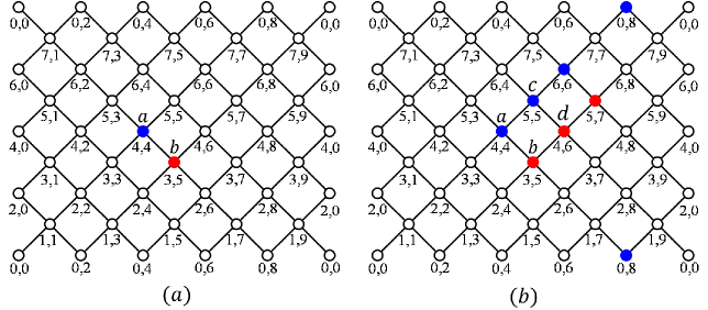
Figure 12: The vertices of $U$ are in blue and the vertices of $W$ are in red. $(a)$ $a\in U\cap{\rm AC}(0,0)$ and $b\in W\cap{\rm AC}(0,2)$. $(b)$ ${\rm AC}(0,0)\subseteq U$ and ${\rm AC}(0,2)\subseteq W$. Notice that a red vertex lies on an isometric path between two blue vertices.

Now, $a\in U\cap{\rm AC}(0,0)$ and $b\in W\cap{\rm AC}(0,2)$. Let $c=(r,r+2)$ and $d=(r+1,r+1)$. Observe that $d$ is adjacent to $a$ and lies in ${\rm AC}(0,0)$. In the same way, $c$ is adjacent to $b$ and lies in ${\rm AC}(0,2)$. Consider $C_{4}$ cycle $\{a,b,c,d\}$. Since $a$ is in $U$ and $b$ is in $W$, vertex $d$ must be in $U$ and vertex $c$ must be in $W$. Otherwise, it will contradict our assumption that $U$ and $W$ are convex. In other words, when $a\in U\cap{\rm AC}(0,2k)$ and $b\in W\cap{\rm AC}(0,2k+2)$, its adjacent vertices $d\in U\cap{\rm AC}(0,2k)$ and $c\in W\cap{\rm AC}(0,2k+2)$. Continuing the same logic, we show that ${\rm AC}(0,0)$ is a subset of $U$ and ${\rm AC}(0,2)$ is a subset of $W$.

Now consider the vertex $(r+r,j+r)$ which is $(2r,j+r)$ = $(0,j+r)$. Notice that $(0,j+r)$ is in $U\cap AC(0,2k)$. Now consider the obtuse path ${\rm OP}((r,r),(0,j+r))$ between $(r,r)$ and $(0,j+r)$. Since the length of ${\rm OP}((r,r),(0,j+r))$ is $r$, it is isometric. Now vertex $b=(r-1,r+1)\in W$ and lies in the isometric path ${\rm OP}((r,r),(0,j+r))$ where $(r,r)$ and $(0,j+r)$ are in $U$. It implies that $U$ is not convex. This is a contradiction.

Initially we assumed that $ab$ is an obtuse edge. If $ab$ is an acute edge, we will argue with obtuse cycles ${\rm OC}(0,0)$ and ${\rm OC}(0,2)$ in the place of ${\rm AC}(0,0)$ and ${\rm AC}(0,0)$. The other case $b$ is $(r+1,r-1)$ is also straightforward. ∎

6 Extension of the cut method

UNDER PREPARATION

The combinatorial graph problems such as embedding of one graph into another graph, computation of Wiener Index, estimating forwarding indices or designing routing algorithms require convex edgecuts. The cut method which is built on convex edgecuts is a powerful tool to solve some graph combinatorial problems such as average distance of a graph, edge forwarding index, embedding and routing algorithms etc [14, 16, 18]. The basic requirement of the cut method is a convex edgecut partition in some forms [17]. The cut method was introduced by Klavžar el al [15]. It was further extended by Chepoi el al [4] in the form of $\ell_{1}$-graphs. The $k$-cut method was designed in the form of quotient graphs by means of $\Theta^{*}$-relation [9, 14, 16].

There are graphs which do not admit convex edgecuts. Notice that an odd cycle admits neither a convex edgecut nor an edgecut partition. However, there are graphs which admit edgecut partitions but do not admit a convex edgecut partition. Villarceau torus is one such graph. Here we extend the convex cut method to graphs which admit edgecut partitions but do not admit a convex edgecut partition.

A partition $\{E_{1},\cdots,E_{p}\}$ of $E$ is said to be an edgecut partition if each $E_{i}$ is an edgecut of $G$ for $i=1,\ldots,p$. A partition $\{E_{1},\cdots,E_{p}\}$ is said to be a convex edgecut partition if each $E_{i}$ is a convex edgecut of $G$ for $i=1,\ldots,p$.

In this paper, $\mathcal{C}$ denotes a set of paths in $G$. When $\mathcal{C}$ contains $|V|(|V|-1)/2$ paths, it is called routing [26]. The congestion $\Pi(G,\mathcal{C},e)$ of an edge $e$ is the number of paths of $\mathcal{C}$ passing through $e$. Given a set $S$ of edges, $\Pi(G,\mathcal{C},S)$ = $\sum_{e\in S}{\Pi(G,\mathcal{C},e)}$. Also, we define $\Pi(G,\mathcal{C})=\max_{e\in E}\Pi(G,\mathcal{C},e)$ and $\Pi(G)=\min_{\mathcal{C}\in G}\Pi(G,\mathcal{C})$

Theorem 6.1.

Let $\mathcal{C}$ denote a set of paths in a graph $G$. Let $\{E_{1},\cdots,E_{p}\}$ be an edgecut partition of $G$ where each $E_{i}$ is a $(U_{i},W_{i})$-edgecut of $G$. Given $\mathcal{C}$ and $\{E_{1},\cdots,E_{p}\}$ of $G$, define the following terms:

$k_{U_{i},W_{i}}$ = $\sum_{x\in U_{i},y\in W_{i},P(x,y)\in\mathcal{C}}{|E_{i}\cap P(x,y)|}$

$k_{U_{i}}$ = $\sum_{x,y\in U_{i},P(x,y)\in\mathcal{C}}{|E_{i}\cap P(x,y)|}$

$k_{W_{i}}$ = $\sum_{x,y\in W_{i},P(x,y)\in\mathcal{C}}{|E_{i}\cap P(x,y)|}$

where $|E_{i}\cap P(x,y)|$ is the number of edges common to $E_{i}$ and $P(x,y)$. Then

$$\sum_{P(x,y)\in\mathcal{C}}{|P(x,y)|}=\sum_{i=1}^{p}{(k_{U_{i},W_{i}}+k_{U_{i}}+k_{W_{i}})}$$

Proof.

It is well-known [26] that $\sum_{P(x,y)\in\mathcal{C}}{|P(x,y)|}$ = $\sum_{i=1}^{p}{\Pi(G,\mathcal{C},E_{i})}$. Consider $E_{i}$ where $E_{i}$ is a $(U_{i},W_{i})$-edgecut. Initially $\Pi(G,\mathcal{C},E_{i})=0$. Now, there are only three possibilities:

1. For $x\in U_{i}$ and $y\in W_{i}$, $\Pi(G,\mathcal{C},E_{i})$ is incremented by $k_{U_{i},W_{i}}$.

2. For $x,y\in U_{i}$, $\Pi(G,\mathcal{C},E_{i})$ is incremented by $k_{U_{i}}$.

3. For $x,y\in W_{i}$, $\Pi(G,\mathcal{C},E_{i})$ is incremented by $k_{W_{i}}$.

Thus, $\Pi(G,\mathcal{C},E_{i})$ = $k_{U_{i},W_{i}}+k_{U_{i}}+k_{W_{i}}$. Hence, $\sum_{P(x,y)\in\mathcal{C}}{|P(x,y)|}$ = $\sum_{i=1}^{p}{\Pi(G,\mathcal{C},E_{i})}$ = $\sum_{i=1}^{p}{(k_{U_{i},W_{i}}+k_{U_{i}}+k_{W_{i}})}$ ∎

Figure 13: $X$ type of edgecuts. The edges of edgecut $S$ are depicted in dotted lines. The deletion of S disconnects $G$ into two connected components $G{U}$ and $G[W]$. The disconnected components $G{U}$ and $G[W]$ are in two different colors.

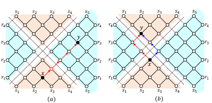
Figure 14: to be added.

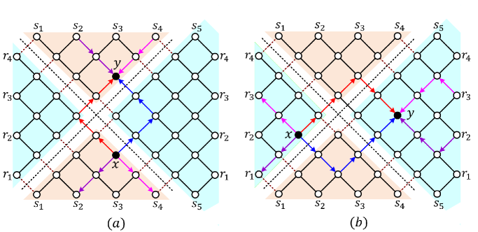
Figure 15: .

7 Computation of Wiener Index of ${\rm VT}(r,s)$

UNDER PREPARATION

Since Villarceau torus does not admit convex partitions, the computation of the Wiener Index of ${\rm VT}(r,s)$ becomes tedious and complicated. Many wonder “Is it worth and required, when an $O(n^{3})$ brute-force algorithm [14, 16, 17, 18] is available to compute Wiener Index of ${\rm VT}(r,s)$?”. The implementation of this brute-force algorithm gives only the value of the Wiener Index and it does not give the formula for the Wiener Index of ${\rm VT}(r,s)$. The objective here is to derive a formula for the Wiener Index of ${\rm VT}(r,s)$ so that this formula will be applied in other combinatorial problems such as graph embedding, forwarding indices and network routing algorithms [18]. In addition, once a formula is derived, the running time of the computation of the Wiener Index becomes $O(1)$ which is constant time.

Even though ${\rm VT}(r,s)$ does not admit any convex edgecuts, it admits edgecuts. Since ${\rm VT}(r,s)$ is bipartite, there are several type of edgecuts. One type of edgecuts is illustrated in Figure 13.

Given a pair $x$ and $y$ of vertices in $G$, an acute isometric $x,y$-path is an isometric path traversing only along acute edges and an obtuse isometric $x,y$-path is an isometric path traversing only along obtuse edges. An acute-obtuse isometric $x,y$-path is an isometric path that traverses along acute edges first and then traverses along obtuse edges until reaching $y$. Similarly, an obtuse-acute isometric $x,y$-path is an isometric path that traverses along obtuse edges first and then traverses along acute edges until reaching $y$.

We partition the set $V\times V$ into three subsets as follows: $T_{1}=\{{x,y}:x,y\in V$ and $\}$ xxxx

Observation 7.1.

Let $x$ and $y$ be a pair of vertices in ${\rm VT}(r,s)$. Let $\{E_{1},\cdots,E_{p}\}$ be an arbitrary edgecut partition of $G$ where each $E_{i}$ is a $(U_{i},W_{i})$-edgecut of $G$.

Case 1: Suppose vertices $x$ and $y$ lie on some ${\rm AP}(0,2k)$ (resp. ${\rm OP}(0,2k)$).

In this case, the isometric $x,y$-path $P(x,y)$ is an acute (resp. obtuse) isometric path. If $x,y\in U_{i}$ (resp. $W_{i}$), then $|E_{i}\cap P(x,y)|=0$. If $x\in U_{i}$ and $y\in W_{i}$, then $|E_{i}\cap P(x,y)|=1$.

Case 2: Suppose $d(x,y)\neq r$ and $d(x,y)\neq s$.

In this case, there is one acute-obtuse isometric $x,y$-path $P_{1}(x,y)$ and one obtuse-acute isometric $x,y$-path $P_{2}(x,y)$ between $x$ and $y$. These two isometric paths do not have common vertices other than $x$ and $y$. Also, $P_{1}(x,y)$ and $P_{2}(x,y)$ form a diamond shape between $x$ and $y$. If $x,y\in U_{i}$ (resp. $W_{i}$), then $|E_{i}\cap P_{1}(x,y)|=|E_{i}\cap P_{2}(x,y)|=0$ or $|E_{i}\cap P_{1}(x,y)|=|E_{i}\cap P_{2}(x,y)|=2$. If $x\in U_{i}$ and $y\in W_{i}$, then $|E_{i}\cap P_{1}(x,y)|=|E_{i}\cap P_{2}(x,y)|=1$.

Case 3: Suppose $d(x,y)=r$ & $d(x,y)\neq s$ (resp. $d(x,y)=s$ & $d(x,y)\neq r)$.

In this case, there is a pair of acute-obtuse isometric $x,y$-path $P_{1}(x,y)$ and obtuse-acute isometric $x,y$-path $P_{2}(x,y)$ which form a diamond shape between $x$ and $y$. Then, there is one more pair of acute-obtuse isometric $x,y$-path $P_{3}(x,y)$ and obtuse-acute isometric $x,y$-path $P_{4}(x,y)$ which form another diamond shape between $x$ and $y$. All these four isometric paths are mutually vertex-disjoint except at $x$ and $y$. If $x,y\in U_{i}$ (resp. $x,y\in W_{i}$), then $|E_{i}\cap P_{1}(x,y)|=|E_{i}\cap P_{2}(x,y)|=2$ and $|E_{i}\cap P_{3}(x,y)|=|E_{i}\cap P_{4}(x,y)|=0$. If $x\in U_{i}$ and $y\in W_{i}$, then $|E_{i}\cap P_{1}(x,y)|=|E_{i}\cap P_{2}(x,y)|=|E_{i}\cap P_{3}(x,y)|=|E_{i}\cap P_{4}(x,y)|=1$.

In Observation 7.1, the case “$d(x,y)=r=s$” does not arise in the rectangular Villarceau torus ${\rm VT}(r,s)$ because $s$ is assumed to be larger than $r$.

8 Congestion-balanced routing

UNDER PREPARATION

The problem of finding optimal congestion-balanced routing in a graph G is equivalent to the problem of finding the edge forward index of $G$ [26]. Thus, the problem of finding a congestion-balanced routing for general graphs is NP-complete [26].

A routing $\mathcal{C}$ is said to be congestion-balanced if $\Pi(G,\mathcal{C},e_{i})$ = $\Pi(G,\mathcal{C},e_{j})$ for every $e_{i}$ and $e_{j}$ in $E(G)$. A routing $\mathcal{C}$ is said to be optimal congestion-balanced if $\Pi(G,\mathcal{C},e_{i})$ = $\Pi(G,\mathcal{C},e_{j})$ = $\dfrac{d_{u,v\in V}d_{G}(u,v)}{|E|}$ for every $e_{i}$ and $e_{j}$ in $E(G)$.

Now we shall demonstrate how Villarceau torus ${\rm VT}(r,s)$ admits an optimal congestion-balanced routing.

References

- [1] R .Blum, Circles on surfaces in the Euclidean 3-space, Lecture Notes in Mathematics, 792(1980) 213–221.
- [2] Eric Baird, Villarceau circles and variable-geometry toroidal coils. Columbia University, USA, July 2018.
- [3] J. Caceres, A. Marquez, O. Oellermann, and M. Puertas, Rebuilding convex sets in graphs, Discrete Mathematics, 297(1-3) (2005) 26–37.
- [4] V. Chepoi, M. Deza, and V. Grishukhin, Clin d’oeil on L1-embeddable planar graphs, Discrete Applied Mathematics 80 (1997) 3–19.
- [5] O. Consa, Helical solenoid model of the electron. Progress in Physics, 14(2) (2018) 80–89.
- [6] H.S.M. Coxeter, Introduction to Geometry, 2nd ed. New York: Wiley, Pages 132–133, 1969.
- [7] L. Dorst, Conformal Villarceau Rotors, Advances in Applied Clifford Algebras, 29 (2019) 44–64, . https://doi.org/10.1007/s00006-019-0960-5
- [8] WU Fei-long, LI Chuan-liang, SHI Wei-xin, WEI Ji-lin, and DENG Lun-hua, Study on the Spiral-Torus Herriott Type Cell, Spectroscopy and Spectral Analysis, 36 (4) (2016) 1051–1055. DOI: 10.3964/j.issn.1000-0593(2016)04-1051-05
- [9] R.L. Graham, and P.M. Winkler, On isometric embeddings of graphs. Transactions of the American Mathematical Society, 288 (1985) 527–536.
- [10] William Guss and Chiping Chen, Equilibrium of self-organized electron spiral toroids, Physics of Plasmas, 9 (8) (2002) 3303–3310. https://doi.org/10.1063/1.1487864
- [11] J. Hefferon and W.E. Clark, Elementary Number Theory, University of South Florida, 2002.
- [12] D. Hestenes, Zitterbewegung structure in electrons and photons, arXiv:1910.11085: General Physics, 24 Jan 2020.
- [13] J. Huret, DNA: molecular structure, Atlas of Genetics and Cytogenetics in Oncology and Haematology, 2006.
- [14] S. Klavžar. A birds eye view of the cut method and a survey of its applications in chemical graph theory. MATCH Communications in Mathematical and in Computer Chemistry, 60 (2008) 255–274.
- [15] S. Klavžar, I. Gutman, and B. Mohar, Labelling of benzenoid systems which reflects the vertex-distance relation. The Journal for Chemical Information and Computer scientists, 35 (1995) 590–593
- [16] S. Klavžar and M.J. Nadjafi-Arani, Wiener index in weighted graphs via unification of *-classes, European Journal of Combinatorics, 36 (2014) 71–76.
- [17] S. Klavžar and G.D. Romih, The Cut Method on Hypergraphs for the Wiener Index, Journal of Mathematical Chemistry, 289 (2023). DOI: https://doi.org/10.1007/s10910-023-01478-4.
- [18] P. Manuel, I. Rajasingh, B. Rajan and H. Mercy, Exact wirelength of hypercube layout on -cube necklace, Journal of Combinatorial Mathematics and Combinatorial Computation, 67 (2008) 67–76.
- [19] P.T. Meijer, Connectivities and diameters of circulant graphs, MSc Thesis, Simon Fraser University, Canada, 1991.
- [20] M.G. Monera and J. Monterde, Building a Torus with Villarceau Sections, Journal for Geometry and Graphics, 15(1) (2011) 93–99.
- [21] K. Olsen and J. Bohr, Geometry of the toroidal N-helix: optimal-packing and zero-twist, New Journal of Physics, 14 (2012) 023063. DOI 10.1088/1367-2630/14/2/023063.
- [22] N. Parthiban, I. Rajasingh, R.S. Rajan, Improved Bounds on Forwarding Index of Networks, Procedia Computer Science, 57 (2015, 592–595.
- [23] D. Roegel, The Villarceau circles in Uhlberger’s staircase (ca. 1580), [Research Report] 2014, HAL-00941465.
- [24] M. Villarceau, ”Théorème sur le tore.” Nouv. Ann. Math. 7 (1848) 345–347.
- [25] J. Watson and F. Crick, A structure for deoxyribose nucleic acid. Nature, 171 (1953) 737–738.
- [26] J. Xu and M. Xu, The forwarding indices of graphs – a survey, Opuscula Mathematica, 33(2) (2013) 345–372.
- [27] M. Yolles and G. Fink. A General Theory of Generic Modeling and Paradigm Shifts. Kybernetes, 44(2) (2015)283–298.
- [28] C. Zhang and K. Nandakumar, Enhancement of Heat Transfer in Laminar Flows Using a Toroidal Helical Pipe, Industrial and Engineering Chemistry Research, Volume 59(9) (2020) 3922–3933, . DOI: 10.1021/acs.iecr.9b04196