Emergent Asymmetry of Precision and Recall for Measuring Fidelity and Diversity of Generative Models in High Dimensions

Abstract

Precision and Recall are two prominent metrics of generative performance, which were proposed to separately measure the fidelity and diversity of generative models. Given their central role in comparing and improving generative models, understanding their limitations are crucially important. To that end, in this work, we identify a critical flaw in the common approximation of these metrics using k-nearest-neighbors, namely, that the very interpretations of fidelity and diversity that are assigned to Precision and Recall can fail in high dimensions, resulting in very misleading conclusions. Specifically, we empirically and theoretically show that as the number of dimensions grows, two model distributions with supports at equal point-wise distance from the support of the real distribution, can have vastly different Precision and Recall regardless of their respective distributions, hence an emergent asymmetry in high dimensions. Based on our theoretical insights, we then provide simple yet effective modifications to these metrics to construct symmetric metrics regardless of the number of dimensions. Finally, we provide experiments on real-world datasets to illustrate that the identified flaw is not merely a pathological case, and that our proposed metrics are effective in alleviating its impact.

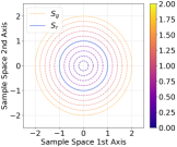
(a) 2-Sphere Setting

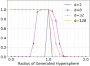
(b) Precision

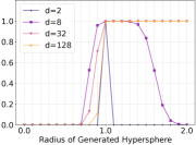
(c) Recall

Figure 1: Asymmetry of Precision and Recall with Hyperspherical supports. (a) Illustrates the setup of the experiment in $d=2$, where the solid blue line denotes the reference unit 2-sphere support, and the dashed lines denote generated 2-sphere supports of varying distances from the reference (radius on colorbar). (b, c) The generated support being outside or inside the reference support results in vastly different measures, becoming more asymmetric as the number of dimensions grows. Same behavior is observed with other radii (see Appendix C).

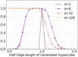
(a) Precision (Hypercube)

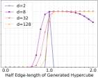
(b) Recall (Hypercube)

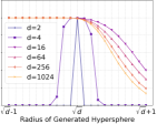
(c) Precision (Gaussian)

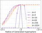
(d) Recall (Gaussian)

Figure 2: Asymmetry of Precision and Recall with Hypercubic supports, and Gaussian spherical supports. (a, b) The reference support is the hypercube of half-edge-length 1. (c, d) The reference support is a hypersphere at $\sqrt{\textrm{d}}$. The generated support being outside or inside the reference support results in vastly different behavior, which becomes more and more asymmetric as dimensions grow.

1 Introduction

Accurately measuring the performance of generative models has become a major challenge due to the rapid growth of their application in downstream tasks – from super-resolution (Pathak et al., 2018), to data-augmentation (Sandfort et al., 2019), and art creation (Rombach et al., 2022). To address this challenge, initially qualitative and heuristic measures of difference between generated samples and real samples were proposed (Arora et al., 2018; Salimans et al., 2016; Hore & Ziou, 2010), followed by more recent moment-based distances (Bińkowski et al., 2018; Heusel et al., 2017) and neural network distances (Karras et al., 2020b; Ravuri & Vinyals, 2019), which could provide a more consistent evaluation with human perception (Lucic et al., 2018). However, these metrics were lacking in one important aspect: separately measuring fidelity and diversity of generated samples. To address this shortcoming, Precision and Recall (Sajjadi et al., 2018), and their later improved versions (Kynkäänniemi et al., 2019), were proposed (henceforth Precision and Recall refers to the improved versions).

Given finite sets of samples $X_{r}$ and $X_{g}$, from a real and a generated distribution, $p_{r}$ and $p_{g}$, Precision measures the fraction of generated samples that fall within the support of the real distribution approximated using $K$-nearest-neighbors (fidelity of generated samples), whereas Recall measures the fraction of real samples that fall within the support of the approximated generated distribution (meaningful diversity of generated samples):

$$\begin{split}\textrm{Precision}&(p_{r},p_{g})=\mathbb{P}_{p_{g}}\left[\hat{S_{r}}\cap S_{g}\right]\\ &\approx\frac{1}{|X_{g}|}\sum_{x_{i}\in X_{g}}1(x_{i}\in\hat{S_{r}})\end{split}$$ (1)

$$\begin{split}\textrm{Recall}&(p_{r},p_{g})=\mathbb{P}_{p_{r}}\left[S_{r}\cap\hat{S_{g}}\right]\\ &\approx\frac{1}{|X_{r}|}\sum_{x_{i}\in X_{r}}1(x_{i}\in\hat{S_{g}})\end{split}$$ (2)

where $1(.)$ is the indicator function, $S_{r}$ and $S_{g}$ are the supports of $p_{r}$ and $p_{g}$, and hat denotes approximation of support by $K$-nearest-neighbors (details in Section 3).

Given the ubiquitous adoption of Precision and Recall in practice, recent works have focused on studying the limitations of these metrics (Naeem et al., 2020; Alaa et al., 2022). In the same spirit, in this work, we identify and formalize a critical flaw in Precision and Recall, namely, that their very interpretations as fidelity and diversity could fail in high dimensions. More specifically, two model distributions with supports $S_{g}$ and $S_{g}^{\prime}$ at equal point-wise distance from the support of the real distribution $S_{r}$, can have vastly different Precision and Recall regardless of their respective distributions $p_{g}$ and $p_{g}^{\prime}$, hence an emergent asymmetry in high dimensions. Even worse, $S_{g}^{\prime}$ can be quite far from $S_{r}$, while $S_{g}$ is very close to $S_{r}$, and yet any $p_{g}^{\prime}$ can achieve much higher Precision (or Recall) compared to any $p_{g}$. Consequently, comparing distributions in high dimensions in terms of Precision and Recall becomes nearly meaningless.

The main contribution of this paper is to empirically and theoretically show the existence of an emergent asymmetry in Precision and Recall, and its consequences in practice. The rest of this paper is organized as follows: we start by providing a motivating example in Section 2 that empirically shows the existence of the asymmetry, and then analytically prove its existence in Section 3; next, in Section 4, we use the insights from the developed theory to design modified versions of Precision and Recall that are symmetric in low and high dimensions; finally, in Section 5, we provide experiments on two real-world datasets, CelebA (Liu et al., 2015) and CIFAR10 (Krizhevsky et al., 2009), to show the existence of the asymmetry in practice, and to illustrate the effectiveness of our proposed metrics. We close this paper with a discussion of related works in Section 6 followed by remaining questions and future directions in Section 7.

2 A Motivating Example

In this section, we will provide a motivating example that illustrates how in high dimensions the expected interpretation of Precision and Recall as measures of fidelity and diversity fails. Consider a real distribution $p_{r}$ whose support $S_{r}$ is the surface of the unit $d-1$ dimensional sphere, and a generated/learnt distribution $p_{g}$ whose support $S_{g}$ is the surface of another $d-1$ dimensional sphere with the same center point, both uniformly distributed. In two dimensions, these supports would be two concentric circles (as in Figure 1a), in three dimensions two concentric spheres, and so forth. Now imagine we start increasing the radius of $S_{g}$ from zero to infinity. The common understanding of Precision and Recall suggests that as $S_{g}$ approaches $S_{r}$ and passes it, we should observe a bump in both Precision and Recall, and otherwise both should be zero. As Figure 1 shows, this expected behavior is correctly observed in low dimensions, however, as the number of dimensions increases we observe a strikingly different behavior: the generated support being slightly outside or inside the real support results in vastly different Precision and Recall, hence an emergent asymmetry in high dimensions. To make sure this is not just a peculiarity of hyperspheres, we repeat the same experiment with hypercubes in Figure 2, and observe the same behavior. We also repeat the experiment for the support of standard Gaussian distributions, which resembles a sphere of radius $\sqrt{d}$, and again observe the same behavior in Figure 2. Using different radii and K values for the K-nearest-neighbors  results in the same behavior as well (Appendices C and D).

This behavior breaks the general intuition of fidelity and diversity assigned to Precision and Recall in high dimensions. For example, a generated distribution that is slightly outside the real distribution, will have much lower Precision than one that is far away from the real distribution but inside, resulting in the misleading conclusion that the much farther latter distribution is actually generating samples with higher fidelity. Similarly, a distribution slightly inside the real distribution will be seen as having a much lower diversity compared to a distribution far outside of the real distribution, according to Recall. These issues are not mere pathological cases and can have practical consequences: when an algorithm tries to match its generated support to that of the high dimensional real data – as is the case in most prominent generative models such as GANs (Goodfellow et al., 2014), VAEs (Kingma & Welling, 2014), and Diffusion Models (Ho et al., 2020) – it would approach the real support from different directions and oscillate near it (Khayatkhoei et al., 2018; Mescheder et al., 2018), at which point Precision and Recall are typically used to choose the trade-off between diversity and fidelity (Kynkäänniemi et al., 2019), and compare models with one another, however, the phenomenon observed in Figures 1 and 2 can render such trade-off decisions based on Precision and Recall meaningless.

3 Emergent Asymmetry in High Dimensions

In this section, our goal is to mathematically explain the asymmetry observed in Section 2 and the mechanisms behind it. Our analysis will be restricted to the case of distributions supported on hyperspheres, however, we will comment on its generality later in this section.

We start by stating the setup for our analysis. We consider reference and generated distributions, $p_{r}$ and $p_{g}$, that are absolutely continuous on their supports $S_{r}$ and $S_{g}$, respectively, and further assume $S_{r}$ is the surface of a $d-1$ dimensional hypersphere. Given a random set of observations $X_{r}=\{x_{i}\}_{i=1}^{N}$ from $p_{r}$, we construct a $K$-nearest-neighbors approximation to the reference support, that is $\hat{S_{r}}=\cup_{i=1}^{N}N_{K}(x_{i})\approx S_{r}$ where $N_{K}(x_{i})$ is the $d$ dimensional ball centered at $x_{i}$ with radius equal to the Euclidean distance of $x_{i}$ from its $K$-th nearest neighbor in $X_{r}$. This constitutes the support approximation typically used for the calculation of Precision and Recall. Now, to explain the behavior observed in Section 2, we will analyze the Precision of $p_{g}$ – the measure of overlap between the approximated reference support and the generated support with respect to the probability measure defined by $p_{g}$ – in two cases: when $p_{g}$ is contained inside and outside of $S_{r}$.

To study the first case, we assume $p_{g}$ has support inside the hypersphere $S_{r}$. More concretely, $S_{g}=B$ where $B$ is the $d$-ball whose boundary is $\partial B=S_{r}$. In this case, the following theorem shows that given a practical number of samples (e.g. $N$ being polynomial in $d$), the Precision will approach 1 with high probability asymptotically in the number of dimensions. Intuitively, this means that in high dimensions, any absolutely continuous distribution contained inside the hypersphere will be completely covered by the approximated reference distribution.

Proposition 3.1.

Given reference and generated distributions $p_{r}$ and $p_{g}$, absolutely continuous on their respective supports $S_{r}$ and $S_{g}$, where $S_{r}$ is a $d-1$ dimensional hypersphere and $S_{g}$ is the $d$ dimensional ball $B$ with boundary $S_{r}$, and the $K$-nearest-neighbors approximation of $S_{r}$ using $N$ samples from $p_{r}$ denoted $\hat{S_{r}}$, if $\lim_{d\rightarrow\infty}N\epsilon^{-d}=0$ $\forall\epsilon>1$, then with arbitrarily high probability we have:

$$\lim_{d\rightarrow\infty}\mathbb{P}_{p_{g}}\left[\hat{S_{r}}\cap S_{g}\right]=1$$ (3)

Proof.

In Appendix A.∎

This result is intuitively expected from the fact that the volume of a hypersphere of any radius asymptotically (in the number of dimensions) tends to zero, however, note that this fact on its own cannot explain the saturating Precision: given arbitrarily many samples we have $\hat{S}_{r}=S_{r}$ and thus $\hat{S_{r}}\cap S_{g}=S_{r}\cap S_{g}=\partial B\cap B$ which has measure zero under $p_{g}$ regardless of the number of dimensions. Therefore, the main reason why Precision saturates in Proposition 3.1 is that the number of samples have a sub-exponential growth in the number of dimensions $d$, which in turn suggests that this behavior is not an intrinsic property of hyperspheres in high dimensions, rather an instance of the curse of dimensionality limiting our approximation ability. Note that since Recall is equal to Precision when swapping the generated and reference distributions (see Equations 1 and 2), the result in Proposition 3.1 readily extends to Recall. Specifically, it explains that Recall will approach 1 with high probability as the number of dimensions grows, when the reference distribution is inside the generated distribution.

Next, we study the second case, where we assume $p_{g}$ has support outside of the hypersphere $S_{r}$. More concretely, we assume $S_{g}$ is inside a $d$-ball $B_{o}$ containing the $d$-ball $B$ whose boundary is $\partial B=S_{r}$, and outside $B$. In this case, the following theorem shows that given a practical number of samples (e.g. $N$ being polynomial in $d$), the Precision will approach 0 with high probability asymptotically in the number of dimensions. Intuitively, this means that in high dimensions, any absolutely continuous distribution contained outside of the hypersphere will have no overlap with the approximated reference distribution.

Proposition 3.2.

Given a reference distribution $p_{r}$ whose support $S_{r}$ is the $d-1$ dimensional hypersphere, a generated distribution $p_{g}$ absolutely continuous on its support $S_{g}$ which is outside the $d$ dimensional ball $B$ with boundary $\partial B=S_{r}$ and inside a $d$ dimensional ball $B_{o}\supset B$, i.e. $S_{g}=B_{o}\setminus(B\setminus\partial B)$, and the $K$-nearest-neighbors approximation of $S_{r}$ using $N$ samples from $p_{r}$ denoted $\hat{S_{r}}$, if $\lim_{d\rightarrow\infty}N\epsilon^{-d}=0$ $\forall\epsilon>1$, then with arbitrarily high probability we have:

$$\lim_{d\rightarrow\infty}\mathbb{P}_{p_{g}}\left[\hat{S_{r}}\cap S_{g}\right]=0$$ (4)

Proof.

In Appendix B.∎

This result also readily extends to Recall by swapping the generated and reference distributions as explained before, that is, Recall will approach 0 with high probability as the number of dimensions grows, when the reference distribution is outside the generated distribution.

There are two main assumptions in the above results that require justification for why they are sensible in practice. First, the assumption of absolutely continuous distributions is sensible when considering the fact that representing the support of distributions in digital computers is subject to numerical rounding errors, which means we can always assume the presence of an infinitesimal amount of noise in the true distribution such that it becomes absolutely continuous. Additionally, various regularization techniques are often used to explicitly avoid close to measure zero supports for $p_{g}$ (Arjovsky & Bottou, 2017). The second assumption is the hyperspherical supports. This is indeed diverging from the real-world situation of complicated manifolds as supports. Nonetheless, we think studying this restricted case provides valuable insights into the behavior of Precision and Recall in practice, because while practical distributions have complicated supports, these supports do share some defining characteristics with hyperspheres, most notably, being closed (compact and without boundary). Considering practical distributions as being supported on manifolds that can be well represented by digital computers, their compactness follows from the set of floating-point numbers being finite, and being without boundary follows from the common assumption that the data manifold is everywhere locally homeomorphic to the same Euclidean space. For a more specific discussion focused on image patches see (Carlsson et al., 2008). Furthermore, we will see in Section 5 that empirical results on real-world datasets are consistent with the behavior we observed and proved for hyperspheres. We conjecture that this behavior is more generally true for any distribution $p_{r}$ supported on the boundary of a compact space, however, we were not able to prove this at present.

While the above results reveal the mechanism behind the asymmetry we observed in Section 2, they also suggest a potential solution: in the proof of Proposition 3.1, we observe that a critical step giving rise to the asymmetric behavior is approximating the support of $p_{r}$ with $K$-nearest-neighbors. If we were to instead approximate the support of $p_{g}$, then we would end up with a setup that resembles that of Proposition 3.2 in that the approximated support is now placed inside the other support. Similarly, the setup of Proposition 3.2 would resemble that of Proposition 3.1 by changing the distribution that is being approximated. As such, it seems possible to maintain the diversity and fidelity interpretations of Precision and Recall, while inverting the asymmetry. In the following section, we will take advantage of this observation to modify Precision and Recall such that they become more symmetric in high dimensions.

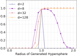
(a) cPrecision (Hypersphere)

(b) cRecall (Hypersphere)

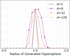
(c) symPrecision (Hypersphere)

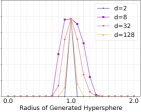
(d) symRecall (Hypersphere)

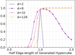
(e) cPrecision (Hypercube)

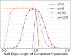
(f) cRecall (Hypercube)

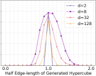
(g) symPrecision (Hypercube)

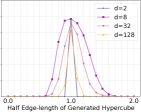
(h) symRecall (Hypercube)

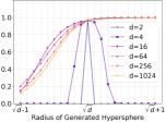
(i) cPrecision (Gaussian)

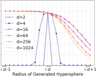
(j) cRecall (Gaussian)

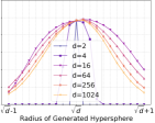
(k) symPrecision (Gaussian)

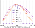
(l) symRecall (Gaussian)

Figure 3: symPrecision and symRecall exhibit symmetric behavior inside or outside the reference support, regardless of the number of dimensions, in contrast to the asymmetry observed in Precision and Recall, and their complements (cPrecision and cRecall). (a, b, c, d) The reference support is the hypersphere of radius 1. (e, f, g, h) The reference support is the hypercube of half-edge-length 1. (i, j, k, l) The reference support is hypersphere at $\sqrt{\textrm{d}}$, following the support of Gaussian distributions.

4 Symmetric Precision and Recall

As we observed in Section 3, the direction of the asymmetry in Precision and Recall is connected to which distribution’s support is approximated with the $K$-nearest-neighbors. Following up on this observation, we can consider complement versions of Precision and Recall, denoted cPrecision and cRecall, where we keep everything in the respective formulas the same except for which distribution is approximated, arriving at the following definitions:

$$\begin{split}\textrm{cPrecision}&(p_{r},p_{g})=\mathbb{P}_{p_{g}}\left[S_{r}\cap\hat{S_{g}}\right]\\ &\approx\frac{1}{|X_{g}|}\sum_{x_{i}\in X_{g}}1(N_{K}(x_{i})\ni\joinrel\in X_{r})\end{split}$$ (5)

$$\begin{split}\textrm{cRecall}&(p_{r},p_{g})=\mathbb{P}_{p_{r}}\left[\hat{S_{r}}\cap S_{g}\right]\\ &\approx\frac{1}{|X_{r}|}\sum_{x_{i}\in X_{r}}1(N_{K}(x_{i})\ni\joinrel\in X_{g})\end{split}$$ (6)

where $\ni\joinrel\in$ denotes non-empty intersection, $1(.)$ is the indicator function, $X_{r}$ and $X_{g}$ are sets of samples from $p_{r}$ and $p_{g}$, $S_{r}$ and $S_{g}$ are their respective supports, $N_{K}(x_{i})$ denotes the $K$-nearest-neighbors neighborhood of $x_{i}$, and hat denotes approximation of support by $K$-nearest-neighbors. In other words, cPrecision measures the fraction of generated samples whose neighborhoods each contains at least one real sample, and cRecall measures the fraction of real samples whose neighborhoods each contains at least one generated sample. The latter has been previously proposed by Naeem et al. (2020) under the name Coverage , to address the problem of sensitivity of Recall to outliers in generated data, while we are not aware of the former being presented in prior works. However, in this discussion, we are interested not in their ability to overcome outliers, rather their asymmetry in high dimensions: as shown in Figure 3, both cPrecision and cRecall exhibit asymmetry in high dimensions similar to Precision and Recall, but with a crucial twist: their asymmetrical behavior is inverted. cPrecision vanishes when $p_{g}$ is inside $p_{r}$ and saturates when outside (opposite the trend in Precision we observed in Figure 2). Conversely, cRecall saturates when $p_{g}$ is inside $p_{r}$ and vanishes when outside (opposite the trend in Recall we observed in Figure 2).

As such, while cRecall and cPrecision cannot fix the asymmetry in high dimensions, their combination with Precision and Recall might. To that end, we can naturally define a more symmetric Precision and Recall by taking the minimum of the corresponding pairs of metrics, which we denote symPrecision and symRecall:

symPrecision $$=\min(\textrm{cPrecision},\textrm{Precision})$$ (7)

symRecall $$=\min(\textrm{cRecall},\textrm{Recall})$$ (8)

The reasoning behind the choice of $\min$ is as follows. We want to convert an asymmetric metric, say $f(x)$, into a symmetric one, say $h(x)$, while maintaining its semantics (here $x$ is a scalar representing the expansion/contraction of the generated support such that at $x=0$ it is equal to the real manifold). To do so, we designed a complement metric $g(x)$ with two properties: first, having the same semantics of diversity or fidelity as $f$ (e.g. Precision and cPrecision both measure fidelity); second, having the inverted asymmetry of $f$, that is, $g(x)=f(-x)$. Now, choosing $h(x)=\min(g(x),f(x))$ makes $h$ readily symmetric, $h(x)=h(-x)$. Instead of $\min$ we could use any function that is invariant under permutations of its variables, however, we chose $\min$ because it can maintain the semantics of $f$ and $g$ by gating between them.

As expected, in Figure 3 we observe that these metrics behave more symmetrically in all experiments, regardless of the number of dimensions. Note that since the proposed metrics simply take the minimum, they do not violate the intended intuition of fidelity and diversity assigned to Precision and Recall, rather extend it to when the supports do not exactly match in high dimensions. In particular, the insensitivity to outliers is maintained since outliers can only artificially inflate Precision or Recall, in which case the minimum will result in the use of cPrecision and/or cRecall which are more robust to outliers (Naeem et al., 2020). Additionally, when the generated and real supports match, since asymptotically (in the number of samples) Precision and Recall are equal to their complements, the symmetric Precision and Recall will also converge to the same asymptotic values. So far, all our empirical evidence have been restricted to synthetic data. In the next section, we will explore whether the asymmetry also emerges in practice.

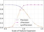
(a) Fidelity (CelebA)

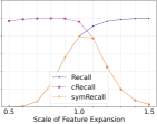
(b) Diversity (CelebA)

(c) Fidelity (CIFAR10)

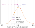
(d) Diversity (CIFAR10)

Figure 4: The effect of scaling the feature space of CelebA and CIFAR10 images with various scaling factors, where scaling of 1 will be the same as no scaling (i.e. the generated and reference supports become equal). While Precision and Recall, and their complements, all exhibit asymmetric behavior, symPrecision and symRecall can achieve symmetric behavior.

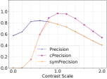
(a) Fidelity (CelebA)

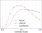
(b) Diversity (CelebA)

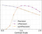
(c) Fidelity (CIFAR10)

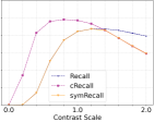
(d) Diversity (CIFAR10)

Figure 5: The effect of increasing the contrast of images of CelebA and CIFAR10 with various scaling factors, where scaling of 1 will be the same as no scaling (i.e. the generated and reference supports become equal). While Precision and Recall, and their complements, all exhibit asymmetric behavior, symPrecision and symRecall can achieve more symmetric behavior (notice the faster decaying tails on both sides for symPrecision and symRecall). The symmetry not being ideal is due to the fact that increasing/decreasing contrast might not move the embedded image manifold with equal rates outward and inward.

5 Real Data Experiments

In this section, we provide two experiments to study the existence of the emergent asymmetry of Precision and Recall in real-world datasets. In these experiments, we use images from CelebA (Liu et al., 2015) at $128\times 128$ resolution, and images from CIFAR10 (Krizhevsky et al., 2009) at $32\times 32$ resolution, and the VGG16 (Simonyan & Zisserman, 2014) pretrained on ImageNet (Deng et al., 2009) to encode the images into embedding space as suggested by Kynkäänniemi et al. (2019). We also consider an alternative random embedding space in Appendix F. In all experiments, both with synthetic data and real data, we use 10,000 random samples from each of the real and generated distributions to compute the metrics, and repeat all experiments five times and report average values with one standard deviation above and below the average (the standard deviation is regularly very small and not discernible in the figures). Additionally, we note that the authors of Precision and Recall suggested $K=3$ in (Kynkäänniemi et al., 2019), whereas follow up work (Naeem et al., 2020) suggested $K=5$ for Coverage (cRecall). We experimented with both values, and observed no significant change in the reported behavior, and therefore chose to report all experiments using $K=5$ in favor of consistency. The code and experiments will be available at https://github.com/mahyarkoy/emergent_asymmetry_pr.

5.1 Scaling the Feature Space

In this experiment, we directly scale the feature space of embedded images, in order to contract and expand the image manifold in the feature space. More specifically, for each set of embedded images using $\phi$, $\{\phi(x_{i})\}_{i=1}^{N}$, we compute the sample mean $\hat{\phi}$, and scale each sample along the direction of the mean, that is, $\phi_{s}(x)=s(\phi(x)-\hat{\phi})+\hat{\phi}$, where $s\in[0.5,1.5]$ is the scaling factor. Each value of $s$, together with a random subset from the training set of the respective datasets embedded with VGG16, is treated as a distinct generative model, whereas the real distribution is the embedded testing set of the respective datasets.

In Figure 4, as we change the scale from 0.5 to 1.5, passing the real distribution’s support at $s=1$, we again observe the asymmetric behavior in Precision and Recall, that is, being inside the real support makes a generative model appear as if it is generating samples of much higher fidelity compared to being on the outside, and vice versa for Recall. In contrast, our proposed metrics, symPrecision and symRecall, exhibit the expected symmetrical behavior, consistent with the interpretation of fidelity and diversity. Note that the image distributions in embedding space have much more complicated supports compared to the synthetic distributions we considered in Section 2, which shows the existence of the asymmetry in real-world distributions.

5.2 Varying Image Contrast

In the previous experiment, we directly scaled the image manifold in the embedding space and observed the asymmetry in metrics, however, the question remains whether the feature space scaling can be realized by actual changes in the image space, or it is a pathological modification unlikely to occur during image generation. The challenge here is that if we use trained generative models, it is unclear how to rigorously determine when models are moving the image support outside/inside the real image support, versus when models are genuinely generating samples that are of high/low fidelity and diversity. To make sure images are actually being moved away (inwards or outwards) from the real image support, we consider a family of generative models that generate by applying a fixed contrast scale $s\in[0,2]$ to randomly chosen images from the training set of real datasets. The real dataset is considered as the testing set of the dataset under study (with no modification to the contrast). With this family of models (each model applying a distinct contrast scale $s$), we can be sure that by increasing and decreasing contrast away from $1$, the generative models’ supports are moving outward and inward from the real image support, respectively.

In Figure 5, we observe the asymmetric behavior in Precision and Recall, showing that it is not only possible, but practical, for a family of generative models to generate samples that have unfairly high/low Precision or Recall. For example, in Figures 5a and 5c, samples of $s=0.4$ contrast, which are washed out, always achieve higher Precision than samples of $s\geq 1$ which are of much higher fidelity (see samples in Figure 6). Similarly, in Figures 5b and 5d, samples of $s=2$, which are extremely over-exposed, always receive higher Recall than samples of $s=0.4$, although both have the same amount of meaningful diversity. In all cases, the use of our proposed metrics alleviate these issues and results in a more symmetric behavior (i.e. faster decaying tails as $s$ approach $0$ and $2$). The remaining asymmetry can be explained by noting that the sensitivity of the embedding network (VGG16) to contrast increase and decrease is not necessarily exactly the same.

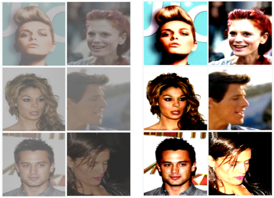
Contrast	$0.4$ $\rightarrow$	$2.0$
Precision	$0.82$ $\pm 0.00$ $\rightarrow$	$0.40$ $\pm 0.00$
Recall	$0.18$ $\pm 0.00$ $\rightarrow$	$0.68$ $\pm 0.01$
symPrecision	$0.15$ $\pm 0.00$ $\rightarrow$	$0.40$ $\pm 0.00$
symRecall	$0.18$ $\pm 0.00$ $\rightarrow$	$0.36$ $\pm 0.01$

Figure 6: Visualizing examples from the contrast varying experiment, where changing the contrast results in a rapid saturation/vanishing in Precision and Recall, consistent with the emergence of asymmetry in high dimensions. The images on the left are deemed to be of much higher fidelity (higher Precision) than the images to the right, which is misleading. Also, The images on the left are considered as capturing less of the diversity of real images than the ones on the right, which again is misleading. Proposed symmetric metrics substantially reduce this unexpected gap, keeping both metrics under 0.5 for both left and right images.

6 Related Works

Heuristic Metrics of Generative Performance. Comparing two sets of images in terms of quality has long been of interest due to its application to compression. Most notable classical methods for this task are PSNR and SSIM which compare images directly in terms of differences in pixel values (Hore & Ziou, 2010), and remain useful to date, in particular to detect whether a generative model is memorizing training samples (Karras et al., 2020a). Divergences between distributions have also been traditionally used to compare generative models, however, since computing likelihood is often intractable in high dimensions, direct use of divergences remain useful mostly in low dimensional setting. A notable example is Inception Score (Salimans et al., 2016) which uses a classifier to construct a tractable likelihood for a set of images over a finite number of class categories, which can then be compared with another set of images using KL divergence. Several other heuristics have also proven useful in probing specific aspects of generative performance: comparing the support size of generative models based on human-guided detection of duplicates (Arora et al., 2018), measuring the amount of high frequency artifacts in generative models by comparing their average spectra (Dzanic et al., 2020; Khayatkhoei & Elgammal, 2022), comparing the linear separability of generative models’ latent spaces and the smoothness of the mapping to image space – denoted Perceptual Path Length – as a surrogate for having learnt the correct generative model (Karras et al., 2018, 2020b), computing the accuracy of a classifier trained to distinguish generated samples from real ones as a measure of distribution mismatch, denoted Neural Net Divergence (Arora et al., 2017), and using improvements from adding generated samples to downstream tasks as a measure of generalization (Ravuri & Vinyals, 2019). Despite each method having its own particular use cases, a shared limitation of them is not providing a direct way of disentangling the differences in diversity and fidelity.

Moment-based Metrics. These metrics compare two sets of images by estimating and comparing their moments in a predetermined feature space. Most notably, Frechet Inception Distance (Heusel et al., 2017), maps the two image sets into the latent space of an Inception Net (Szegedy et al., 2016) pretrained on ImageNet (Deng et al., 2009), and compare their first and second moments. Kernel Inception Distance (Bińkowski et al., 2018) allows for comparing higher moments in the same latent space. Moment-based methods, similar to heuristic methods, cannot distinguish lack of diversity from lack of fidelity. In order to address this drawback, manifold-based metrics were introduced.

Manifold-based Metrics. These metrics compare two sets of images by estimating and comparing their support manifold in an embedding space, typically using VGG16 (Simonyan & Zisserman, 2014) pretrained on ImageNet (Deng et al., 2009). The manifold of each set is estimated as the union of the $K$-nearest-neighbors balls centered at each data point, in a similar construction as Isomap (Tenenbaum et al., 2000). How to compare the two estimated manifolds results in various metrics. Improved Precision and Recall, compute the fraction of model samples that fall in the data manifold and the fraction of data samples that fall in the model manifold, respectively – these methods were originally proposed to improve the estimation of similar concepts proposed by Sajjadi et al. (2018). Naeem et al. (2020) discovered a sensitivity to outliers in Precision and Recall, and therefore proposed modifications denoted Density and Coverage, where Density measures the average number of real data neighborhoods that cover any generated data sample normalized by the neighborhood’s expected size ($K$ of $K$-nearest-neighbors), and Coverage measures the fraction of generated data samples whose neighborhood contain any real data sample. More recently, Alaa et al. (2022) proposed $\alpha$/$\beta$ Precision and Recall, which aimed to generalize these metrics such that instead of comparing the whole supports of real and generated data, their supports are first partitioned into different levels of likelihood, and then Precision and Recall are computed for each pair of the partition. This would allow a more granular comparison between distributions, and also addresses the problem of sensitivity to outliers. However, to compute the partitions, they use a trained embedding network to maximally squeeze the data manifold into a sphere, which raises the possibility of distorting the semantic meaning of distances in the data manifold, that is, some distances could arbitrarily collapse.

The Curse of Dimensionality. Our analysis is a particular manifestation of the curse of dimensionality. The effect of growing dimensions on distance concentration and meaningfulness of nearest neighbors has been extensively explored in classical settings, specially in the context of kernels (François et al., 2007; Evangelista et al., 2006; Aggarwal et al., 2001; Beyer et al., 1999). In particular, the fact that the ratio of distance variance to distance to mean of i.i.d. random variables vanishes with increasing number of dimensions, and consequently distances between all points appear similar, which will break down the utility of many kernel based estimations. A phenomenon very closely related to our analysis in this paper, is the emergence of hubs in high dimensional Gaussian distributions. Hubs refer to points that are close to a very large number of other samples from the Gaussian distribution under a $K$-nearest-neighbors notion of closeness, much larger than the average number of neighborhoods that contain any point (Radovanovic et al., 2010). Our theoretical analysis extends the known reach of the curse of dimensionality, by showing how it affects the overlap between distributions supported on hyperspheres.

7 Conclusion

In this work, we identified a critical flaw in the common approximation of Precision and Recall using $K$-nearest-neighbors, denoted emergent asymmetry: in high dimensions, moving the generated distribution slightly outwards or inwards away from the real distribution’s support can lead to vastly different values of Precision and Recall in each direction. We proved this asymmetry for distributions supported on hyperspheres, and empirically showed its emergence in synthetic and real-world datasets. We also proposed modifications to Precision and Recall to reduce the effect of the asymmetry in high dimensions. Our findings suggest several interesting directions for future research. First, as we conjectured in Section 3 and observed in the experiments of Section 5, the asymmetry is not restricted to distributions with hyperspherical supports; identifying the necessary assumptions on a space for the emergence of the asymmetry is a valuable future direction. Second, while we proved the asymmetry asymptotically, deriving bounds in the finite case would provide more granular insights. Finally, while we showed the existence of the emergent asymmetry in the widely-used Improved Precision and Recall metrics, the extent to which it affects other metrics of generative performance remains to be explored.

Appendix A Proof of Proposition 3.1

Proof.

We start by making two redundant assumptions which we will relax later: 1) the distributions $p_{g}$ and $p_{r}$ are uniformly distributed over their respective supports $S_{g}$ and $S_{r}$; and 2) we are constructing the approximate support using first nearest neighbor ($K=1$). Note that $S_{g}$ is the $d$ dimensional ball $B$ of radius $R$, $S_{r}$ is the $d-1$ dimensional hypersphere at its boundary $\partial B=S_{r}$, and $\hat{S}_{r}$ denotes the $K$-nearest-neighbors approximation of $S_{r}$ using a set of $N$ i.i.d. observations $X_{r}=\{x_{i}\}_{i=1}^{N}$ from $p_{r}$, that is, $\hat{S_{r}}=\cup_{i=1}^{N}N_{K}(x_{i})$ where $N_{K}(x_{i})$ is the $d$-ball centered at $x_{i}$ with radius equal to the Euclidean distance of $x_{i}$ from its $K$-th nearest neighbor in $X_{r}$.

The direction of the proof is as follows: we consider the event that there exists a sample from $p_{r}$ with its Euclidean nearest neighbor distance greater or equal to $R\sqrt{2}$, that is:

$$\{\exists x^{*}\in X_{r}:\min_{x\neq x^{*},x\in X_{r}}||x^{*}-x||\geq R\sqrt{2}\}$$ (9)

and show that under this event, the support of $p_{g}$ will be completely covered by the approximate support of $p_{r}$ as $d\rightarrow\infty$. Then, we compute the probability of this event under $p_{r}$ and observe that it saturates with $d\rightarrow\infty$, concluding the proof.

At a distance $R\sqrt{2}$, the neighborhood of $x^{*}$ intersects $\partial B$ at its equator, therefore the volume of $B$ not covered by $N_{K}(x^{*})$ is less than or equal to the volume of the hyperspherical cap of $B$ at $\phi<\frac{\pi}{2}$ (strictly less than $\frac{\pi}{2}$ because the overlap volume is strictly larger than the hemisphere’s volume):

$$V(B\setminus N_{K}(x^{*}))=V(B)-V(N_{K}(x^{*})\cap B)\leq V(B^{cap}_{\phi<\frac{\pi}{2}})$$ (10)

where hyperspherical cap is defined as the smaller part when a hyperplane cuts a hypersphere of the same number of dimensions into two parts at a colatitude angle $0<\phi\leq\frac{\pi}{2}$ (e.g. $\phi=\frac{\pi}{2}$ would give the two hemispheres). The volume of this hyperspherical cap has the following closed form (Li, 2011):

$${V(B^{cap}_{\phi}})=\frac{1}{2}V_{d}(R)I_{\sin^{2}\phi}(\frac{d+1}{2},\frac{1}{2})$$ (11)

where $I$ is the regularized incomplete beta function, and $V_{d}(R)$ is the volume of the $d$ dimensional ball of radius $R$. Additionally, we can approximate $I$ as follows for large $d$ (omitting higher order terms in $\sin\phi<1$):

$$I_{\sin^{2}\phi}(\frac{d+1}{2},\frac{1}{2})=\frac{\beta(\sin^{2}\phi;\frac{d+1}{2},\frac{1}{2})}{\beta(\frac{d+1}{2},\frac{1}{2})}\approx\frac{\frac{(\sin^{2}\phi)^{\frac{d+1}{2}}}{\frac{d+1}{2}}}{\Gamma(\frac{1}{2})(\frac{d+1}{2})^{-\frac{1}{2}}}=C\sqrt{\frac{(\sin\phi)^{2(d+1)}}{d+1}}$$ (12)

where $\beta$, $\Gamma$ are the beta (incomplete and complete) and gamma functions, respectively, the numerator is due to series expansion, and the denominator is due to Stirling’s approximation. We use C to represent a non-unique constant value in our discussions (which might change between two different formulas). Now, we can compute the probability of $B\setminus N_{K}(x^{*})$ with respect to $p_{g}$ as the ratio of volumes (since we assumed $p_{g}$ to be uniformly distributed on $B$):

$$\mathbb{P}_{p_{g}}\left[B\setminus N_{K}(x^{*})\right]=\frac{V(B)-V(N_{K}(x^{*})\cap B)}{V(B)}\leq C\sqrt{\frac{(\sin\phi)^{2(d+1)}}{d+1}}$$ (13)

At this point we can relax the requirement that $p_{g}$ is uniform, by noting that any absolutely continuous probability measure on $B$ must be within a constant factor of the measure produced by the uniformly distributed measure (due to Radon-Nikodym theorem), therefore the above inequality holds regardless of the uniform assumption (albeit with different constants). Next, since $x^{*}$ is not the only sample used to construct the approximate manifold $\hat{S_{r}}$, and from Equation 13, we have:

$$\mathbb{P}_{p_{g}}\left[\hat{S_{r}}\cap S_{g}\right]=\mathbb{P}_{p_{g}}\left[\hat{S_{r}}\cap B\right]\geq\mathbb{P}_{p_{g}}\left[N_{K}(x^{*})\cap B\right]\geq 1-C\sqrt{\frac{(\sin\phi)^{2(d+1)}}{d+1}}$$ (14)

where the right hand side tends to 1 as $d\rightarrow\infty$, so we arrive at:

$$\lim_{d\rightarrow\infty}\mathbb{P}_{p_{g}}\left[\hat{S_{r}}\cap S_{g}\right]=1$$ (15)

So far we showed that under the event $\{\exists x^{*}\in X_{r}:\min_{x\neq x^{*},x\in X_{r}}||x^{*}-x||\geq R\sqrt{2}\}$, the support of $p_{g}$ will be completely covered by the approximate support of $p_{r}$. What remains is to compute the probability of this event and observe how it behaves with $d$. First, note that to have one sample whose nearest neighbor is more than $R\sqrt{2}$ away, we must have at least one sample from which all the other samples are at least $R\sqrt{2}$ away, hence the following:

$$\mathbb{P}_{X_{r}\sim p_{r}}\left[\exists x^{*}\in X_{r}:\min_{x\neq x^{*},x\in X_{r}}||x^{*}-x||\geq R\sqrt{2}\right]$$ (16)

$$=\mathbb{P}_{X_{r}\sim p_{r}}\left[\exists x^{*}\in X_{r},\forall x\neq x^{*}\in X_{r}:||x^{*}-x||\geq R\sqrt{2}\right]$$ (17)

$$=(1-\mathbb{P}_{p_{r}}\left[||x^{*}-x||<R\sqrt{2}\right])^{N-1}$$ (18)

Then for the inner event we have:

$$\mathbb{P}_{p_{r}}\left[||x^{*}-x||<R\sqrt{2}\right]=\frac{A(B^{cap}_{\phi<\frac{\pi}{2}})}{A(S_{r})}$$ (19)

since $p_{r}$ is uniformly distributed on $\partial B$, and $A(B^{cap}_{\phi<\frac{\pi}{2}})$ denotes the area of the hyperspherical cap of $B$ at colatitute angle $\phi<\frac{\pi}{2}$. This area has the following closed form (Li, 2011):

$${A(B^{cap}_{\phi}})=\frac{1}{2}A_{d}(R)I_{\sin^{2}\phi}(\frac{d-1}{2},\frac{1}{2})$$ (20)

where $I$ is the regularized incomplete beta function, and $A_{d}(R)$ is the area of the $d$ dimensional ball of radius $R$. Using the approximation mentioned in Equation 12, we arrive at (omitting higher order terms in $\sin\phi<1$):

$$\mathbb{P}_{p_{r}}\left[||x^{*}-x||<R\sqrt{2}\right]\approx C\sqrt{\frac{(\sin\phi)^{2(d-1)}}{d-1}}$$ (21)

At this point we can also relax the requirement that $p_{r}$ is uniform, by once again noting that any absolutely continuous probability measure on $\partial B$ must be within a constant factor of the measure produced by the uniformly distributed measure, therefore the above equality becomes an inequality ($\leq$) and holds regardless of the uniform assumption (albeit with different constants). What remains is to apply series expansion to Equation 18 (omitting higher order terms in $p_{r}$):

$$\mathbb{P}_{X_{r}\sim p_{r}}\left[\exists x^{*}\in X_{r}:\min_{x\neq x^{*},x\in X_{r}}||x^{*}-x||\geq R\sqrt{2}\right] =(1-\mathbb{P}_{p_{r}}\left[||x^{*}-x||<R\sqrt{2}\right])^{N-1}$$ (22)

$$\approx 1-(N-1)\mathbb{P}_{p_{r}}\left[||x^{*}-x||<R\sqrt{2}\right]$$ (23)

$$\geq 1-CN\sqrt{\frac{(\sin\phi)^{2(d-1)}}{d-1}}$$ (24)

Now, we note that for $\lim_{d\rightarrow\infty}N\epsilon^{-d}=0$ $\forall\epsilon>1$, i.e. number of samples less than exponential in $d$, the above tends to 1 as $d\rightarrow\infty$:

$$\lim_{d\rightarrow\infty}\mathbb{P}_{X_{r}\sim p_{r}}\left[\exists x^{*}\in X_{r}:\min_{x\neq x^{*},x\in X_{r}}||x^{*}-x||\geq R\sqrt{2}\right]=1$$ (25)

Finally, we relax the assumption of $K=1$ for the $K$-nearest-neighbors approximation of $S_{r}$, since increasing $K$ will strictly increase the overlap between the supports. ∎

Appendix B Proof of Proposition 3.2

Proof.

We start by making a redundant assumption which we will later relax: that the distributions $p_{g}$ and $p_{r}$ are uniformly distributed over their respective supports $S_{g}$ and $S_{r}$. Note that we have assumed $S_{g}=B_{o}\setminus(B\setminus\partial B)$, where $B$ and $B_{o}$ are $d$ dimensional balls such that $B\subset B_{o}$ and $\partial B=S_{r}$. We denote by $R_{o}$ and $R$ the respective radii of $B_{o}$ and $B$, and $\hat{S}_{r}$ denotes the $K$-nearest-neighbors approximation of $S_{r}$ using a set of i.i.d. observations $X_{r}=\{x_{i}\}_{i=1}^{N}$ from $p_{r}$, that is, $\hat{S}_{r}=\cup_{i=1}^{N}N_{K}(x_{i})$ where $N_{K}(x_{i})$ is the $d$-ball centered at $x_{i}$ with radius equal to the Euclidean distance of $x_{i}$ from its $K$-th nearest neighbor in $X_{r}$. Throughout the proof, we consider the largest $K$ (farthest neighbor) since decreasing $K$ strictly reduces the overlap between the supports.

The direction of the proof is as follows: we consider the event that the farthest neighbor for any sample in $X_{r}$ is within an Euclidean distance of $R\sqrt{2}$, that is:

$$\{\forall x^{*}\in X_{r}:\max_{x\neq x^{*},x\in X_{r}}\lVert x^{*}-x\rVert\leq R\sqrt{2}\}$$ (26)

and show that under this event, the support of $p_{g}$ will have almost no overlap with the approximate support of $p_{r}$ as $d\rightarrow\infty$. Then, we compute the probability of this event under $p_{r}$ and observe that it saturates with $d\rightarrow\infty$, concluding the proof.

Under the above event, since the farthest neighbor of any sample $x^{*}\in X_{r}$ is within $R\sqrt{2}$, the approximate support is covered by the union of $d$-balls of radius $R\sqrt{2}$ placed at the observed samples in $X_{r}$, denoted $B_{R\sqrt{2}}(x^{*})$, and using the assumption of uniform $p_{g}$ we have:

$$\mathbb{P}_{p_{g}}\left[\hat{S}_{r}\cap S_{g}\right]\leq N\mathbb{P}_{p_{g}}\left[B_{R\sqrt{2}}(x^{*})\cap S_{g}\right]\leq N\mathbb{P}_{p_{g}}\left[B_{R\sqrt{2}}(x^{*})\cap B_{o}\right]=N\frac{V(B_{R\sqrt{2}}(x^{*})\cap B_{o})}{V(B_{o})-V(B)}$$ (27)

Now we consider two cases. First, when $R_{o}>R\sqrt{2}$, we can write:

$$\mathbb{P}_{p_{g}}\left[\hat{S}_{r}\cap S_{g}\right]\leq N\frac{V(B_{R\sqrt{2}})}{V(B_{o})-V(B)}=\frac{N}{(\frac{R_{o}}{R\sqrt{2}})^{d}-(\frac{1}{\sqrt{2}})^{d}}$$ (28)

and then under the assumption of $\frac{R_{o}}{R\sqrt{2}}>1$, if $\lim_{d\rightarrow\infty}N\epsilon^{-d}=0$ $\forall\epsilon>1$, i.e. the number of samples less than exponential in $d$, the above tends to 0 as $d\rightarrow\infty$.

Second, we consider the case where $R_{o}\leq R\sqrt{2}$ and compute an upper bound for the intersection volume $V(B_{R\sqrt{2}}(x^{*})\cap B_{o})$. To do so, we consider the triangle formed by the centers of the three balls $B_{o},B,B_{R\sqrt{2}}(x^{*})$, and denote the length of the respective sides as $\delta_{ob},\delta_{b*},\delta_{o*}$ corresponding to the distances between the centers of the balls. The intersection volume $V(B_{R\sqrt{2}}(x^{*})\cap B_{o})$ is maximized when the length $\delta_{o*}$ is minimized. From the triangle inequality we have $\delta_{o*}\geq|\delta_{b*}-\delta_{ob}|$, and from $x^{*}\in S_{r}=\partial B$ we have $\delta_{b*}=R$, so it follows that $\delta_{o*}\geq|R-\delta_{ob}|$. Furthermore, from $B\subset B_{o}$ we have $\delta_{ob}\leq R_{o}-R$ and thus $R-\delta_{ob}\geq 2R-R_{o}$, and then from the second case assumption of $R_{o}\leq R\sqrt{2}<2R$ it follows that $\delta_{o*}\geq 2R-R_{o}$. Therefore, we can compute the maximum of $V(B_{R\sqrt{2}}(x^{*})\cap B_{o})$ as the volume of intersection between two $d$-balls of radii $R\sqrt{2}$ and $R_{o}$ with centers at a distance of $2R-R_{o}=\min\delta_{o*}$.

This intersection is consisted of two $d$ dimensional hyperspherical caps, one on $B_{R\sqrt{2}}(x^{*})$ at colatitude angle $\phi_{*}$, and another on $B_{o}$ at colatitude angle $\phi_{o}$. We first show that both angles are acute, by showing that the intersection triangle formed by the centers of the two intersecting balls and a point of intersection, whose sides are of length $R_{o},R\sqrt{2},2R-R_{o}$, is an acute triangle. The largest side of this triangle has length $R\sqrt{2}\geq R_{o}>2R-R_{o}$, and $2R^{2}<R_{o}^{2}+(2R-R_{o})^{2}$, so its acuteness follows from the Pythagorean theorem. The two acute colatitude angles can be computed using Pythagorean equality on the triangle’s altitude:

$$\sin^{2}\phi_{o} =1-\frac{(R_{o}-R)^{4}}{(2R-R_{o})^{2}R_{o}^{2}}$$ (29)

$$\sin^{2}\phi_{*} =1-\frac{(3R-2R_{o})^{2}}{2(2R-R_{o})^{2}}$$ (30)

Now we can use the formula in Equation 11 for the volume of hyperspherical cap at collatitude angle $\phi<\frac{\pi}{2}$ to compute the volume of intersection:

$$\mathbb{P}_{p_{g}}\left[\hat{S_{r}}\cap S_{g}\right]\leq N\frac{V(B_{R\sqrt{2}}(x^{*})\cap B_{o})}{V(B_{o})-V(B)}\leq\frac{NV(B_{\phi_{o}<\frac{\pi}{2}}^{cap})}{V(B_{o})-V(B)}+\frac{NV(B_{\phi_{*}<\frac{\pi}{2}}^{cap})}{V(B_{o})-V(B)}$$ (31)

For the first term, using the approximation in Equation 12 (omitting higher order terms in $\sin\phi_{o}<1$), we have:

$$\frac{NV(B_{\phi_{o}}^{cap})}{V(B_{o})-V(B)}\approx\frac{CN}{2\sqrt{d+1}}\frac{(\frac{R_{o}}{R})^{d}(\sin^{2}\phi_{o})^{\frac{d+1}{2}}}{(\frac{R_{o}}{R})^{d}-1}$$ (32)

For the second term, again using the approximation in Equation 12 (omitting higher order terms in $\sin\phi_{*}<1$), we have:

$$\frac{NV(B_{\phi_{*}}^{cap})}{V(B_{o})-V(B)}\approx\frac{CN}{2\sqrt{d+1}}\frac{(\sqrt{2})^{d}(\sin^{2}\phi_{*})^{\frac{d+1}{2}}}{(\frac{R_{o}}{R})^{d}-1}=\frac{CN}{2\sqrt{2}\sqrt{d+1}}\frac{(2\sin^{2}\phi_{*})^{\frac{d+1}{2}}}{(\frac{R_{o}}{R})^{d}-1}$$ (33)

where for the numerator we can show that $\sqrt{2\sin^{2}\phi_{*}}<\frac{R_{o}}{R}$ as follows:

$$2\sin^{2}\phi_{*}-\frac{R_{o}^{2}}{R^{2}}=2-\frac{(3R-2R_{o})^{2}}{(2R-R_{o})^{2}}-\frac{R_{o}^{2}}{R^{2}}=\frac{-(R_{o}-R)^{4}}{(2R-R_{o})^{2}R^{2}}<0$$ (34)

When $\lim_{d\rightarrow\infty}N\epsilon^{-d}=0$ $\forall\epsilon>1$, i.e. the number of samples less than exponential in $d$, both Equations 32 and 33 tend to 0 as $d\rightarrow\infty$, because $\sin\phi_{o}<1$ and $\sqrt{2\sin^{2}\phi_{*}}<\frac{R_{o}}{R}$, respectively.

At this point, we can relax the requirement that $p_{g}$ is uniform, by noting that any absolutely continuous probability measure on $S_{g}$ must be within a constant factor of the measure produced by the uniformly distributed measure (due to Radon-Nikodym theorem). This concludes the first part of the proof that $\mathbb{P}_{p_{g}}\left[\hat{S_{r}}\cap S_{g}\right]=0$ as $d\rightarrow\infty$ under the event in Equation 26.

What remains is to compute the probability of the event in Equation 26 under $p_{r}$. This can be computed as the probability that given any sample $x^{*}\in X_{r}$, all other samples in $X_{r}$ fall within a distance of $R\sqrt{2}$ from $x^{*}$:

$$\mathbb{P}_{X_{r}\sim p_{r}}\left[\forall x^{*}\in X_{r}:\max_{x\neq x^{*},x\in X_{r}}\lVert x^{*}-x\rVert\leq R\sqrt{2}\right]=(1-\mathbb{P}_{p_{r}}\left[\lVert x^{*}-x\rVert>R\sqrt{2}\right])^{N-1}$$ (35)

where for the inner event, given the uniform assumption on $p_{r}$, we have:

$$\mathbb{P}_{p_{r}}\left[\lVert x^{*}-x\rVert>R\sqrt{2}\right]=\frac{A(B^{cap}_{\phi<\frac{\pi}{2}})}{A(S_{r})}$$ (36)

and the rest of the proof follows the exact steps that connect Equations 19 and 25, concluding that for any absolutely continuous $p_{r}$ and the number of samples less than exponential in $d$, we have $\mathbb{P}_{X_{r}\sim p_{r}}\left[\forall x^{*}\in X_{r}:\max_{x\neq x^{*},x\in X_{r}}\lVert x^{*}-x\rVert\leq R\sqrt{2}\right]=1$ as $d\rightarrow\infty$.

∎

Appendix C Experiments with Varying Radii

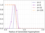
(a) Precision (R=0.5)

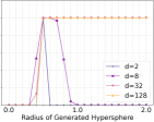
(b) Recall (R=0.5)

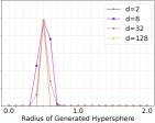
(c) symPrecision (R=0.5)

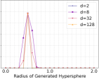
(d) symRecall (R=0.5)

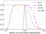
(e) Precision (R=2)

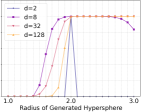
(f) Recall (R=2)

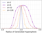
(g) symPrecision (R=2)

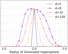
(h) symRecall (R=2)

(i) Precision (R=8)

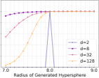
(j) Recall (R=8)

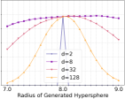
(k) symPrecision (R=8)

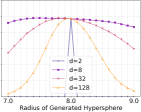
(l) symRecall (R=8)

Figure 7: Hyperspherical reference and generated supports of varying radii at $K=5$ of $K$-nearest-neighbors.

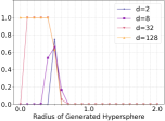
(a) Precision (R=0.5)

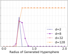
(b) Recall (R=0.5)

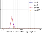
(c) symPrecision (R=0.5)

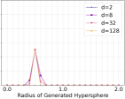
(d) symRecall (R=0.5)

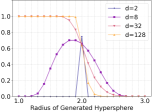
(e) Precision (R=2)

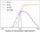
(f) Recall (R=2)

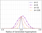
(g) symPrecision (R=2)

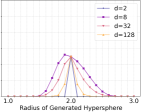
(h) symRecall (R=2)

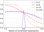
(i) Precision (R=8)

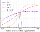
(j) Recall (R=8)

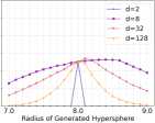
(k) symPrecision (R=8)

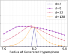
(l) symRecall (R=8)

Figure 8: Hyperspherical reference and generated supports of varying radii at $K=1$ of $K$-nearest-neighbors.

Appendix D Experiments with Varying K of K-Nearest Neighbors

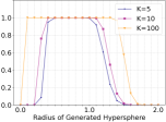
(a) Precision (d=16)

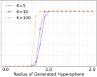
(b) Recall (d=16)

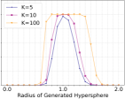
(c) symPrecision (d=16)

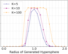
(d) symRecall (d=16)

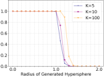
(e) Precision (d=64)

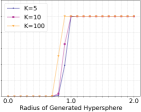
(f) Recall (d=64)

(g) symPrecision (d=64)

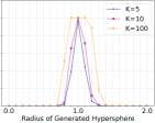
(h) symRecall (d=64)

Figure 9: Hyperspherical reference and generated supports of varying $K$-nearest-neighbors approximations at radius 1. Larger $K$ results in loss of resolution in the manifold approximation, hence the saturated behavior near the reference support (near R=1). The asymmetry in Precision and Recall emerges regardless of $K$, consistent with the proposed theory.

Appendix E Experiments with Varying Number of Samples

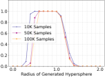
(a) Precision (d=16)

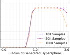
(b) Recall (d=16)

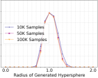
(c) symPrecision (d=16)

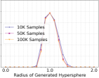
(d) symRecall (d=16)

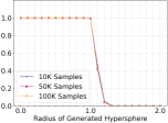
(e) Precision (d=64)

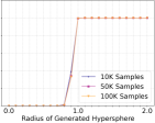
(f) Recall (d=64)

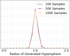
(g) symPrecision (d=64)

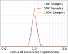
(h) symRecall (d=64)

Figure 10: Hyperspherical reference and generated supports of varying number of samples at radius 1 and $K=5$. Larger number of samples in lower dimensions reduces the asymmetry (note the shrinking tails in $d=16$), however, in higher dimensions it has little to no effect (for $d>64$ the change becomes visually imperceptible in the plots). This is consistent with the proposed theory, which suggests the asymmetry emerges unless the number of samples grows at least exponentially in the number of dimensions.

Appendix F Experiments with Random Embedding for CelebA and CIFAR10

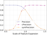
(a) Fidelity (CelebA)

(b) Diversity (CelebA)

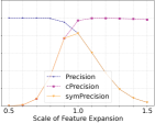
(c) Fidelity (CIFAR10)

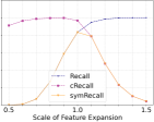
(d) Diversity (CIFAR10)

Figure 11: Repeating the scaling feature space experiment of Section 5.1 using the random R64 embedding of images as proposed by Naeem et al. (2020) instead of the common pretrained VGG16 (Kynkäänniemi et al., 2019). The results are consistent with Figure 4.

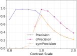
(a) Fidelity (CelebA)

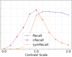
(b) Diversity (CelebA)

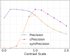
(c) Fidelity (CIFAR10)

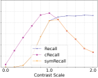
(d) Diversity (CIFAR10)

Figure 12: Repeating the varying contrast experiment of Section 5.2 using the random R64 embedding of images as proposed by Naeem et al. (2020) instead of the common pretrained VGG16 (Kynkäänniemi et al., 2019). The results are consistent with Figure 5.

References

- Aggarwal et al. (2001) Aggarwal, C. C., Hinneburg, A., and Keim, D. A. On the surprising behavior of distance metrics in high dimensional space. In Database Theory—ICDT 2001: 8th International Conference London, UK, January 4–6, 2001 Proceedings 8, pp. 420–434. Springer, 2001.
- Alaa et al. (2022) Alaa, A., Van Breugel, B., Saveliev, E. S., and van der Schaar, M. How faithful is your synthetic data? sample-level metrics for evaluating and auditing generative models. In International Conference on Machine Learning, pp. 290–306. PMLR, 2022.
- Arjovsky & Bottou (2017) Arjovsky, M. and Bottou, L. Towards principled methods for training generative adversarial networks. In International Conference on Learning Representations, 2017.
- Arora et al. (2017) Arora, S., Ge, R., Liang, Y., Ma, T., and Zhang, Y. Generalization and equilibrium in generative adversarial nets (GANs). In Precup, D. and Teh, Y. W. (eds.), Proceedings of the 34th International Conference on Machine Learning, volume 70 of Proceedings of Machine Learning Research, pp. 224–232. PMLR, 06–11 Aug 2017.
- Arora et al. (2018) Arora, S., Risteski, A., and Zhang, Y. Do GANs learn the distribution? some theory and empirics. In International Conference on Learning Representations, 2018.
- Beyer et al. (1999) Beyer, K., Goldstein, J., Ramakrishnan, R., and Shaft, U. When is “nearest neighbor” meaningful? In Database Theory—ICDT’99: 7th International Conference Jerusalem, Israel, January 10–12, 1999 Proceedings 7, pp. 217–235. Springer, 1999.
- Bińkowski et al. (2018) Bińkowski, M., Sutherland, D. J., Arbel, M., and Gretton, A. Demystifying MMD GANs. In International Conference on Learning Representations, 2018.
- Carlsson et al. (2008) Carlsson, G., Ishkhanov, T., De Silva, V., and Zomorodian, A. On the local behavior of spaces of natural images. International journal of computer vision, 76:1–12, 2008.
- Deng et al. (2009) Deng, J., Dong, W., Socher, R., Li, L.-J., Li, K., and Fei-Fei, L. Imagenet: A large-scale hierarchical image database. In 2009 IEEE conference on computer vision and pattern recognition, pp. 248–255. Ieee, 2009.
- Dzanic et al. (2020) Dzanic, T., Shah, K., and Witherden, F. Fourier spectrum discrepancies in deep network generated images. In Advances in Neural Information Processing Systems, 2020.
- Evangelista et al. (2006) Evangelista, P. F., Embrechts, M. J., and Szymanski, B. K. Taming the curse of dimensionality in kernels and novelty detection. In Applied soft computing technologies: The challenge of complexity, pp. 425–438. Springer, 2006.
- François et al. (2007) François, D., Wertz, V., and Verleysen, M. The concentration of fractional distances. IEEE Transactions on Knowledge and Data Engineering, 19(7):873–886, 2007.
- Goodfellow et al. (2014) Goodfellow, I., Pouget-Abadie, J., Mirza, M., Xu, B., Warde-Farley, D., Ozair, S., Courville, A., and Bengio, Y. Generative adversarial nets. In Advances in neural information processing systems, pp. 2672–2680, 2014.
- Heusel et al. (2017) Heusel, M., Ramsauer, H., Unterthiner, T., Nessler, B., and Hochreiter, S. Gans trained by a two time-scale update rule converge to a local nash equilibrium. Advances in neural information processing systems, 30, 2017.
- Ho et al. (2020) Ho, J., Jain, A., and Abbeel, P. Denoising diffusion probabilistic models. Advances in Neural Information Processing Systems, 33:6840–6851, 2020.
- Hore & Ziou (2010) Hore, A. and Ziou, D. Image quality metrics: Psnr vs. ssim. In 2010 20th international conference on pattern recognition, pp. 2366–2369. IEEE, 2010.
- Karras et al. (2018) Karras, T., Laine, S., and Aila, T. A style-based generator architecture for generative adversarial networks. ieee. In CVF Conference on Computer Vision and Pattern Recognition, 2018.
- Karras et al. (2020a) Karras, T., Aittala, M., Hellsten, J., Laine, S., Lehtinen, J., and Aila, T. Training generative adversarial networks with limited data. Advances in Neural Information Processing Systems, 33:12104–12114, 2020a.
- Karras et al. (2020b) Karras, T., Laine, S., Aittala, M., Hellsten, J., Lehtinen, J., and Aila, T. Analyzing and improving the image quality of stylegan. In Proceedings of the IEEE/CVF conference on computer vision and pattern recognition, pp. 8110–8119, 2020b.
- Khayatkhoei & Elgammal (2022) Khayatkhoei, M. and Elgammal, A. Spatial frequency bias in convolutional generative adversarial networks. In Proceedings of the AAAI Conference on Artificial Intelligence, volume 36, pp. 7152–7159, 2022.
- Khayatkhoei et al. (2018) Khayatkhoei, M., Singh, M. K., and Elgammal, A. Disconnected manifold learning for generative adversarial networks. Advances in Neural Information Processing Systems, 31, 2018.
- Kingma & Welling (2014) Kingma, D. P. and Welling, M. Auto-encoding variational bayes. In International Conference on Learning Representations, 2014.
- Krizhevsky et al. (2009) Krizhevsky, A., Hinton, G., et al. Learning multiple layers of features from tiny images. 2009.
- Kynkäänniemi et al. (2019) Kynkäänniemi, T., Karras, T., Laine, S., Lehtinen, J., and Aila, T. Improved precision and recall metric for assessing generative models. Advances in Neural Information Processing Systems, 32, 2019.
- Li (2011) Li, S. Concise formulas for the area and volume of a hyperspherical cap. Asian Journal of Mathematics and Statistics, 4(1):66–70, 2011.
- Liu et al. (2015) Liu, Z., Luo, P., Wang, X., and Tang, X. Deep learning face attributes in the wild. In Proceedings of International Conference on Computer Vision (ICCV), December 2015.
- Lucic et al. (2018) Lucic, M., Kurach, K., Michalski, M., Gelly, S., and Bousquet, O. Are gans created equal? a large-scale study. Advances in neural information processing systems, 31, 2018.
- Mescheder et al. (2018) Mescheder, L., Geiger, A., and Nowozin, S. Which training methods for gans do actually converge? In International conference on machine learning, pp. 3481–3490. PMLR, 2018.
- Naeem et al. (2020) Naeem, M. F., Oh, S. J., Uh, Y., Choi, Y., and Yoo, J. Reliable fidelity and diversity metrics for generative models. In International Conference on Machine Learning, pp. 7176–7185. PMLR, 2020.
- Pathak et al. (2018) Pathak, H. N., Li, X., Minaee, S., and Cowan, B. Efficient super resolution for large-scale images using attentional gan. In 2018 IEEE International Conference on Big Data (Big Data), pp. 1777–1786. IEEE, 2018.
- Radovanovic et al. (2010) Radovanovic, M., Nanopoulos, A., and Ivanovic, M. Hubs in space: Popular nearest neighbors in high-dimensional data. Journal of Machine Learning Research, 11(sept):2487–2531, 2010.
- Ravuri & Vinyals (2019) Ravuri, S. and Vinyals, O. Classification accuracy score for conditional generative models. Advances in neural information processing systems, 32, 2019.
- Rombach et al. (2022) Rombach, R., Blattmann, A., Lorenz, D., Esser, P., and Ommer, B. High-resolution image synthesis with latent diffusion models. In Proceedings of the IEEE/CVF Conference on Computer Vision and Pattern Recognition, pp. 10684–10695, 2022.
- Sajjadi et al. (2018) Sajjadi, M. S., Bachem, O., Lucic, M., Bousquet, O., and Gelly, S. Assessing generative models via precision and recall. Advances in neural information processing systems, 31, 2018.
- Salimans et al. (2016) Salimans, T., Goodfellow, I., Zaremba, W., Cheung, V., Radford, A., and Chen, X. Improved techniques for training gans. Advances in neural information processing systems, 29, 2016.
- Sandfort et al. (2019) Sandfort, V., Yan, K., Pickhardt, P. J., and Summers, R. M. Data augmentation using generative adversarial networks (cyclegan) to improve generalizability in ct segmentation tasks. Scientific reports, 9(1):1–9, 2019.
- Simonyan & Zisserman (2014) Simonyan, K. and Zisserman, A. Very deep convolutional networks for large-scale image recognition. arXiv preprint arXiv:1409.1556, 2014.
- Szegedy et al. (2016) Szegedy, C., Vanhoucke, V., Ioffe, S., Shlens, J., and Wojna, Z. Rethinking the inception architecture for computer vision. In Proceedings of the IEEE conference on computer vision and pattern recognition, pp. 2818–2826, 2016.
- Tenenbaum et al. (2000) Tenenbaum, J. B., Silva, V. d., and Langford, J. C. A global geometric framework for nonlinear dimensionality reduction. science, 290(5500):2319–2323, 2000.