Listener Model for the PhotoBook Referential Game
with CLIPScores as Implicit Reference Chain

Abstract

PhotoBook is a collaborative dialogue game where two players receive private, partially-overlapping sets of images and resolve which images they have in common. It presents machines with a great challenge to learn how people build common ground around multimodal context to communicate effectively. Methods developed in the literature, however, cannot be deployed to real gameplay since they only tackle some subtasks of the game, and they require additional reference chains inputs, whose extraction process is imperfect. Therefore, we propose a reference chain-free listener model that directly addresses the game’s predictive task, i.e., deciding whether an image is shared with partner. Our DeBERTa-based listener model reads the full dialogue, and utilizes CLIPScore features to assess utterance-image relevance. We achieve $>$77% accuracy on unseen sets of images/game themes, outperforming baseline by $>$17 points.

1 Introduction

PhotoBook Haber et al. (2019) is a collaborative dialogue game of two players. In a game round, each player receives 6 images of an identical theme—the two largest objects in all images share the same categories, e.g., dog, car, etc. The players have some of their images in common. Their goal is to communicate through text dialogue, and individually mark 3 privately highlighted images as either common (i.e., shared with partner) or different. A full game lasts 5 rounds. After each round, some of each player’s images are replaced with different ones under the same theme. Images may reappear in later rounds after being swapped out. This game setup encourages building and leveraging common ground with multimodal contexts, which humans are known to do to facilitate conversation Clark and Wilkes-Gibbs (1986); Brennan and Clark (1996). Fig. 1 displays an example of a PhotoBook game.

Models proposed in past works on the dataset Haber et al. (2019); Takmaz et al. (2020) are unable to realistically play the game due to several reasons: (i) they only address subtasks in the game whose time span is one utterance, rendering it unnecessary for the models to keep track of the entire game’s, or round’s, progress; (ii) the models operate on additional input of reference chains, i.e., past utterances referring to each image, whose (rule-based) extraction process is imperfect and hence complicates learning and evaluation; and, (iii) utterances outside of reference chains, e.g., ‘I don’t have that one’, may also be important pieces of information.

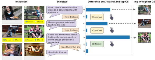
Figure 1: A round of PhotoBook game with dialogue, player marking actions, corresponding images, and CLIPScore (i.e., CS) difference between top and 2nd-top scoring images w.r.t. the utterance. A player needs to figure out whether their partner has each of the 3 target (i.e., highlighted) images through text dialogue.

To address the drawbacks above, we propose a full (i.e., able to play real games), reference chain-free listener model, which accepts all dialogue utterances of a round and the 6 context images, and predicts whether the 3 target (highlighted) images are common/different. Our listener model is based on a pretrained DeBERTa Transformer He et al. (2021). To incorporate visual context, CLIPScores Hessel et al. (2021) between each utterance and the 6 given images are infused with DeBERTa hidden states. We employ CLIPScore as it offers strong prior knowledge about the relevance of an utterance to each of the 6 images, which may serve as a soft, implicit version of reference chain used in previous studies. Also, we chose DeBERTa since it is one of the top performers in the SuperGLUE benchmark Sarlin et al. (2020) which provides a reasonably-sized ($\sim$100M parameters) version to suit our purpose and computation resources. We further devise a label construction scheme to create dense learning signals. Our model scores a $>$77% accuracy on the novel listener task and improves by $>$17% (absolute) over the baseline adapted from Takmaz et al. (2020). Our code is available at github.com/slSeanWU/photobook-full-listener.

2 Related Work

In typical collaborative dialogue tasks, two agents (i.e., players) hold incomplete or partially overlapping information and communicate through text to reach a predefined goal. The task-oriented setup enables simple evaluation for dialogue systems via task success rate, instead of resorting to costly human evaluation. Tasks and datasets proposed in the literature focus either on set logic He et al. (2017), image understanding De Vries et al. (2017); Haber et al. (2019), or spatial reasoning Udagawa and Aizawa (2019). They challenge dialogue systems to process multiple modalities, discard irrelevant information, and build common ground. Researchers have utilized graph neural networks He et al. (2017), vision-and-language Transformers Lu et al. (2019); Tu et al. (2021), and pragmatic utterance generation Frank and Goodman (2012); Fried et al. (2021) to tackle the tasks.

To our knowledge, there has not been a system that fully addresses the PhotoBook task. It may be particularly challenging due to the setup with multiple highly similar images and an unbounded set of information (e.g., scene, actions) the images may contain. Previous PhotoBook works targeted two subtasks: reference resolution Haber et al. (2019); Takmaz et al. (2020) and referring utterance generation Takmaz et al. (2020). The former resolves which of the 6 context images an utterance is referring to, while the latter generates an informative utterance for a pre-selected image. Proposed models take in extracted reference chains—whose rule-based extraction processes try to identify which utterances speak about each of the images. To obtain such chains, Haber et al. (2019) broke the dialogue into segments using a set of heuristics based on player marking actions. Takmaz et al. (2020), on the other hand, computed each utterance’s BERTScore Zhang et al. (2019) and METEOR Banerjee and Lavie (2005) respectively against ground-truth MSCOCO captions Lin et al. (2014), and VisualGenome attributes Krishna et al. (2017) of each image to match (at most) one utterance per round to an image.

As for the reference resolution task, Haber et al. (2019) employed LSTM encoders. One (query) encoder takes a current dialogue segment, while the other (i.e., context encoder) receives the 6 images’ ResNet features, and the associated reference chain segments. Dot products between query encoder output and 6 context encoder outputs are taken to predict the image the current segment refers to. Takmaz et al. (2020) largely kept the setup, but they used BERT Devlin et al. (2019) embeddings and contextualized utterances via weighted averaging instead of LSTMs.

Takmaz et al. (2020) claimed an 85% reference resolution accuracy, but they also reported an 86% precision on reference chain extraction, making it difficult to conclude whether prediction errors are due to model incompetence, or incorrect input data/labels. (We find that some parts of extracted reference chains either point to the wrong image or provide no information at all.) Yet, we do agree that keeping track of which images have been referred to is vital for the game. Therefore, we aim to build a full listener model that does not depend on explicit reference chains, but gathers such information from implicit hints given by an image-text matching model, i.e., CLIP Radford et al. (2021).

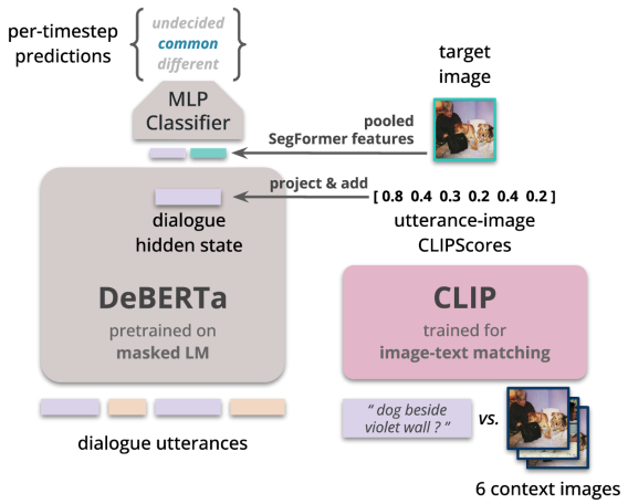
Figure 2: Overview of our listener model. A DeBERTa Transformer He et al. (2021) encodes all utterances of a game round. Utterance-level CLIPScores Hessel et al. (2021) w.r.t. each image (i.e., an $\mathbb{R}^{6}$ vector) get projected and summed with hidden states of all timesteps corresponding to that utterance. Then, a 2-layer MLP takes in pooled SegFormer Xie et al. (2021) features of the target image ($\in\mathbb{R}^{512}$) and DeBERTa output to predict whether the image is common, different, or undecided at every token timestep.

3 Method

3.1 Functionality of CLIPScore

Based on CLIP vision-and-language Transformer Radford et al. (2021), CLIPScore Hessel et al. (2021) is a reference-free metric to measure semantic image-text similarity. On image captioning, Hessel et al. (2021) showed that CLIPScore correlates better with human judgment than reference-dependent metrics like BERTScore Zhang et al. (2019) and SPICE Anderson et al. (2016).

In our pilot study, we find that the CLIPScore of an utterance-image pair is particularly high when the utterance describes the image (see Fig. 1 for example). These score peaks thus form an implicit reference chain for the dialogue, giving strong hints on whether the mentioned images are common/different when seen with subsequent partner feedback (e.g., ‘I have that one’). Also, the reference chain extraction method in Takmaz et al. (2020) achieves higher precision (86%$\rightarrow$93%) and recall (60%$\rightarrow$66%) when we simply replace its core scoring metrics with CLIPScore. The findings above show that CLIPScore captures well the utterance-image relationships in PhotoBook, and hence should be helpful to our listener model.

Computation-wise, reference chain extraction algorithms in the literature either rely on complex turn-level heuristics Haber et al. (2019), or compute multiple external metrics (i.e., BERTScore and METEOR) Takmaz et al. (2020). More importantly, they have to wait until completion of a round to compute the chains. Our utterance-level CLIPScores can be computed on the fly as utterances arrive, and are relatively time-efficient as they involve only one model (i.e., CLIP) and that batch computation may be used to increase throughput.

Modeling-wise, reference chain extraction explicitly selects which utterances the listener model should see, so when it is wrong, the model either sees something irrelevant, or misses important utterances. On the other hand, utterance-level CLIPScores resemble using a highlighter to mark crucial dialogue parts for the model. Even when CLIPScores are sometimes inaccurate, the model could still access the full dialogue to help its decisions.

3.2 The Full Listener Model

3.2.1 Inputs

An overview of our listener model is depicted in Fig. 2. Our model operates on three types of input features, which collectively represent a game round from one of the players’ perspective:

$$\text{Dialogue tokens:}\;\mathcal{X} =\{\bm{x}_{k}\in\mathcal{W}^{|\mathcal{T}_{k}|}\}_{k=1}^{K}$$ (1)

$$\text{CLIPScores:}\;\mathcal{C} =\{\bm{c}_{k}\in\mathbb{R}^{6}\}_{k=1}^{K}$$ (2)

$$\text{Image features:}\;\mathcal{V} =\{\bm{v}_{j}\in\mathbb{R}^{512}\}_{j=1}^{6}$$ (3)

We use $k$, $j$ to index utterances and images respectively. $\mathcal{W}$ is the text token vocabulary, and $\mathcal{T}_{k}=\{t_{k,\text{start}},\dots,t_{k,\text{end}}\}$ is the corresponding token timesteps for the $k^{\text{th}}$ utterance. To the start of each utterance, we prepend either a [CLS] or [SEP] token to distinguish whether it comes from the player itself or the partner. All utterances are concatenated to form one text input sequence to our model. CLIPScore vectors ($\bm{c}_{k}$’s) are computed in a per-utterance manner, i.e., between one utterance and each of the 6 images. Images are represented by the pooled features from SegFormer Xie et al. (2021). It is trained on semantic image segmentation Zhou et al. (2017), and hence should encode crucial visual information for the game, i.e., objects in the scene and their spatial relationships.

3.2.2 Labels and Output

Rather than training the model to predict just once after seeing the entire dialogue, we construct labels for all timesteps, forming a label sequence $\bm{y}_{j}\in\mathcal{L}^{T}$, where $T=\sum_{k}|\mathcal{T}_{k}|$, for each target image, where $\mathcal{L}$ is the label set. As there are only 3 target images out of the 6, we also only have 3 such label sequences ($\bm{y}_{j}$’s) for a training instance. At each timestep $t$, the label of a target image, $y_{j,t}\in\mathcal{L}$, is one of $\{\textit{undecided},\textit{common},\textit{different}\}$. It always starts as undecided, changes to common or different at the moment of player marking action, and remains there for the rest of the dialogue. Our model’s output for a (target) image $j$ at timestep $t$ is hence a distribution $\bm{\hat{y}}_{j,t}\in\mathbb{R}^{3}$, which is a temporary belief about that image. Also, we apply causal masking on DeBERTa self-attention. Such a labeling and masking scheme creates dense learning signals—our model must judge an image at every timestep based on growing dialogue context.

3.2.3 Model Components

The backbone of our model is a pretrained base DeBERTa He et al. (2021), which takes in concatenated utterances $\mathcal{X}=\{\bm{x}_{k}\in\mathcal{W}^{|\mathcal{T}_{k}|}\}_{k=1}^{K}=\{x_{t}\in\mathcal{W}\}_{t=1}^{T}$, and contextualizes them into hidden states:

$$\mathcal{H}^{(l)}=\{\bm{h}^{(l)}_{t}\in\mathbb{R}^{d}\}_{t=1}^{T}\,,\;\;l\in\{1,\dots,L\}\,,$$ (4)

where $d$ ($=\,$768) is DeBERTa’s hidden size, and $l$ is layer index (# layers $L=\,$12). We do not adopt vision-and-language Transformers Lu et al. (2019); Wang et al. (2022) for they are pretrained on ‘single image-short text’ pairs, which mismatches our scenario. Following Wu and Yang (2022)’s recommendation on feeding time-varying conditions to Transformers, utterance-level CLIPScores (i.e., $\mathcal{C}$) are projected and summed with DeBERTa hidden states at all layers:

$$\mathcal{H}^{(l)}\leftarrow\;\{\mathcal{H}_{\mathcal{T}_{k}}^{(l)}=\bm{h}^{(l)}_{t\in\mathcal{T}_{k}}+\bm{W}_{\text{proj}}\,\bm{c}_{k}\,\}_{k=1}^{K}\,,$$ (5)

where $\bm{W}_{\text{proj}}\in\mathbb{R}^{d\times 6}$ is a learnable matrix.

To make predictions, we place a 2-layer MLP (with GELU activation) on top of DeBERTa. It takes in the concatenation of the pooled target image features and the last-layer DeBERTa hidden state, and produces a distribution over the label set $\mathcal{L}=\{\textit{undecided},\textit{common},\textit{different}\}$:

$$\bm{\hat{y}}_{j,t}=\mathrm{MLP}_{\mathbb{R}^{512+d}\rightarrow\mathbb{R}^{3}}([\bm{{v}}_{j};\bm{h}^{(L)}_{t}])\,.$$ (6)

We add learnable positional embeddings to $\bm{{v}}_{j}$’s to make our model aware of the target image’s index.

	valid	test
Random guess	50.0	50.0
Modified Takmaz et al. (2020)	64.2$\>\pm$ 1.7	59.0$\>\pm$ 0.7
w/ CLIPScore ref chains	65.0$\>\pm$ 1.4	59.7$\>\pm$ 0.8
Ours	84.8$\>\pm$ 1.3	77.3$\>\pm$ 0.3
a. $+$ VisAttn	75.0$\>\pm$ 0.6	69.8$\>\pm$ 3.3
b. $-$ CLIPScore	70.7$\>\pm$ 1.1	64.8$\>\pm$ 1.5
c. $-$ CLIPScore $+$ VisAttn	69.8$\>\pm$ 1.1	64.9$\>\pm$ 0.4
d. $-$ Dense learning signals	59.4$\>\pm$ 1.8	55.9$\>\pm$ 0.9
Human	95.0	94.5

Table 1: Listener model accuracy (%) of baselines and our model (full & ablated versions). StDev of 3 runs with fixed seeds shown after $\pm$. Pairwise bootstrap tests corroborate ($p<\,$ .001) that our full model outperforms all baselines and ablated versions. Human is the accuracy annotators achieved during dataset creation. (VisAttn: cross-attention to patch features of 6 context images.)

4 Experiments and Results

Our listener model is trained with the maximum likelihood estimation (MLE) loss function:

$$\mathbb{E}_{(\mathcal{X},\mathcal{C},\mathcal{V},\mathcal{Y})\in\mathcal{D}_{\text{train}}}\sum_{j,t}-\log p_{\bm{\hat{y}}_{j,t}}(y_{j,t}\,|\,\mathcal{X},\mathcal{C},\bm{v}_{j}),$$ (7)

where $\mathcal{D}_{\text{train}}$ is the training split, and $\mathcal{Y}$ is the set of label sequences associated with a data instance. The same images/themes are guaranteed not to appear in multiple dataset splits. We refer readers to Appendix A for more implementation and training details. Evaluation metric adopted here is accuracy measured at the end of dialogue, i.e., at evaluation, we ignore temporary beliefs in the chat. To set a baseline, we modify the reference resolution model in Takmaz et al. (2020) to suit our listener task.

Table 1 lists the evaluation results. Our method outperforms baseline by 17$\sim$20 percentage points, closing the gap to human performance by more than half. Examining the ablations, we can observe that both removing CLIPScore inputs and dense learning signals (i.e., having labels at all timesteps, see Sec. 3.2.2) cause serious accuracy degradation, indicating their essentiality in our model, and that a pretrained Transformer does not trivially beat a fully MLP-based baseline. Besides, though adding cross-attention to image features (i.e., ablations a. & c.) seems to be a more intuitive way to involve visual context, it leads to more severe overfitting and hence does not help in our case. We provide more detailed observations on our best-performing model’s behavior and outputs in Appendix G.

5 Conclusions and Future Work

In this paper, we first discussed why it is difficult to deploy existing reference chain-dependent PhotoBook models to real gameplay, and demonstrated that CLIPScore’s image-text matching capability may provide implicit reference chains to the task. We then developed a novel listener model that is reference chain-free, and able to realistically play the game given text dialogue and the set of context images, just as what human players see. The model is built on a DeBERTa Transformer backbone, and brings in visual context by infusing utterance-level CLIPScores with its hidden states. On the newly proposed full listener task, i.e., predicting whether an image is shared with partner, our model achieves 77$\sim$84% accuracy on unseen sets of images, surpassing baseline Takmaz et al. (2020) by over 17 points. Ablation studies also showed that feeding CLIPScores and imposing dense learning signals are both indispensable to our model’s success.

Future studies may leverage parameter-efficient transfer learning He et al. (2022); Houlsby et al. (2019); Hu et al. (2022); Perez et al. (2018) to cope with image data scarcity of PhotoBook (and potentially other datasets and tasks). It is also interesting to develop a speaker model that uses temporary beliefs from our listener model and takes pragmatics Frank and Goodman (2012); Fried et al. (2021) into account to generate informative responses. Pairing such a model with our listener model may complete the collaborative dialogue task end-to-end.

6 Limitations

The PhotoBook dataset has a very limited number of images (i.e., 360) and image combinations (i.e., 5 per game theme), which may lead to undesirable overfitting behavior as we discuss in Appendix E. Also, since our model depends heavily on CLIP Radford et al. (2021), it is likely to inherit CLIP’s biases and weaknesses. For example, Radford et al. (2021) mentioned that CLIP fails to perform well on abstract or more complex tasks, such as counting or understanding spatial relationships between objects. Finally, whether our listener model can be easily applied/adapted to productive real-world tasks (e.g., automated customer service with image inputs) requires further exploration.

Appendices

Appendix A Details on Model Implementation and Training

Our listener model’s implementation is based on HuggingFace’s DeBERTa module. The 16$\times$16 (512-dimensional) patch features for each context image are extracted from last encoder layer of the publically released SegFormer-b4 model trained on ADE20k Zhou et al. (2017) semantic image segmentation dataset. CLIPScores between utterances and images are computed using the official repository which employs Vision Transformer-base (ViT-B/32) Dosovitskiy et al. (2021) as the image encoder. Our listener model adds $\sim$1M trainable parameters to the 12-layer base DeBERTa backbone, which originally has 100M parameters.

We split our dataset to train/validation/test with a 70/10/20 ratio and make sure that a theme (i.e., categories of the 2 largest objects appearing in all 6 context images in a game round), and hence any image, does not lie across multiple splits. Since a game round has 2 perspectives (i.e., players), it also spawns 2 instances. Rounds in which players make mistakes, or mark images before the first utterance, are filtered out. We finally obtain 13.7K/1.8K/3.7K instances for each of the splits respectively.

We train the model for 100 epochs and early stop on validation accuracy with 10 epochs of patience. AdamW Loshchilov and Hutter (2018) optimizer with $10^{-3}$ weight decay is used. We warm up the learning rate linearly for 500 steps to $2\times 10^{-5}$, and then linearly decay it to $0$ for the rest of the training. Batch size is set to 16. Training takes around 8 hours to complete on an NVIDIA A100 GPU with 40G memory. For fair comparison across model settings and baselines, we randomly draw 3 seeds and run training on all settings/baselines with them.

	Dataset size	Inputs	Tgt. resolution	SoTA E2E performance	SoTA techniques
MutualFriends He et al. (2017)	11K dialogues	Text (tabular)	Bilateral	96% He et al. (2017)	GNN, LSTM
GuessWhat?! De Vries et al. (2017)	150K dialogs, 66K imgs	Text & image	Unilateral	63% Tu et al. (2021)	ViLBERT
OneCommon Udagawa and Aizawa (2019)	5K dialogues	Text & dots on plane	Bilateral	76% Fried et al. (2021)	LSTM, CRF, RSA
PhotoBook Haber et al. (2019)	12.5k dialogs, 360 imgs	Text & 6 images	Bilateral	No complete system yet	ResNet, LSTM

Table 2: Some datasets for collaborative dialogue tasks. Bilateral (or unilateral) ‘Tgt. resolution’ means whether it requires both (or just one) players to figure out the entities/objects they should focus on. (Performance is measured by end-to-end task success.)

Appendix B Details on the Attempt to Infuse Visual Features with Cross Attention

In addition to fusing CLIPScores into DeBERTa self-attention, we also attempt cross-attending DeBERTa hidden states to the 6 context images’ SegFormer features to incorporate visual information.

We denote the SegFormer patch features by:

$$\mathcal{V}^{\mathrm{(pt)}}=\{\bm{v}_{j,p}^{\mathrm{(pt)}}\in\mathbb{R}^{512}\}_{j=1,\;p=1}^{6,\;\;\;\;\;16\times 16}\,,$$ (8)

where $j,p$ respectively indexes images and patches. All image features (16$\times$16$\times$6$\,=\,$1536 vectors) are concatenated into one long sequence for the DeBERTa hidden states (with text & CLIPScore information) to cross-attend to. As a sequence with length over 1.5K would lead to large memory footprint for attention operations, we downsample the patch features (to 8$\times$8$\times$6 $\,=\,$ 384 vectors) through strided 2D group convolution before feeding them to cross-attention, i.e.,

$$\mathcal{\dot{V}}^{{\mathrm{(pt)}}}=\; \mathrm{StridedGroupConv2D}(\mathcal{V}^{{\mathrm{(pt)}}})$$ (9)

$$\mathcal{H}^{(l)}\leftarrow\; \mathrm{Attention}(\mathcal{H}^{(l)},\mathcal{\dot{V}^{\mathrm{(pt)}}},\mathcal{\dot{V}^{\mathrm{(pt)}}})\,,$$ (10)

where $\mathcal{H}^{(l)}$ is the $l^{\text{th}}$-layer DeBERTa hidden states. The patch features in $\mathcal{\dot{V}^{\mathrm{(pt)}}}$ are further mean-pooled to form inputs (for target images), i.e., $\mathcal{V}$, to our final MLP classifier (please check Eqn. 3 & 6, too):

$$\mathcal{V}=\{\bm{v}_{j}\}_{j=1}^{6}=\{\>\mathrm{MeanPool}(\{\bm{\dot{v}}^{\mathrm{(pt)}}_{j,p}\}_{p=1}^{8\times 8})\>\}_{j=1}^{6}\\$$ (11)

In the model settings whose performance is reported in Table 1 (i.e., ablations a. & c.), we place two such cross-attention layers with tied weights before all DeBERTa self-attention layers to give the model more chances to digest and reason with visual inputs. Doing so introduces 8M new trainable parameters (cf. $\sim$1M for our best model). We also try to place these cross-attention layers later in the model in unreported experiments. However, when using visual cross-attention, our listener model always suffers more from overfitting—lower training loss but worse evaluation accuracy.

Appendix C Adapting Takmaz et al. (2020)’s Model for Our Listener Task

The reference resolution model in Takmaz et al. (2020) contains two components: query encoder and context encoder:

• Query encoder: takes in BERT embeddings of a current utterance and the concatenation of 6 context images’ ResNet features, and outputs one representation through learnable weighted averaging (across utterance timesteps).

• Context encoder: encodes each of the 6 images and the associated reference chain (i.e., past utterances referring to that image) separately. The average of each reference chain utterance’s BERT embeddings gets summed with that image’s ResNet features to form the context representation for that image.

The model is based on fully-connected layers entirely. Finally, dot products between the query representation and 6 context representations are taken, and the $\mathrm{arg\,max}$ is deemed the referent image of the current utterance.

To adapt their model to our full listener task, we feed to the query encoder BERT embeddings of the whole round of dialogue and ResNet features of the target image instead. We mean-pool the 6 context encoder representations, concatenate this pooled representation with the query representation, and apply a GELU-activated 2-layer MLP (similar to our model’s) on top of the concatenated representations to predict whether the target image is common or different. This modified baseline model can hence be trained using an objective similar to our model’s (i.e., Eqn. 7). Note that there is no dense learning signal for this adapted baseline, as the representation from query encoder is already pooled across timesteps.

Appendix D Experiments on CLIPScore Injection Layers

Layers fed	valid	test
[emb]	72.4$\>\pm$ 0.7	66.3$\>\pm$ 0.5
[emb, 1st]	78.7$\>\pm$ 1.4	71.9$\>\pm$ 1.6
[emb, 1st$\sim$5th]	82.2$\>\pm$ 1.0	76.5$\>\pm$ 1.1
[4th$\sim$9th]	82.7$\>\pm$ 0.7	76.1$\>\pm$ 0.6
[7th$\sim$12th]	83.0$\>\pm$ 0.6	75.9$\>\pm$ 0.6
All layers	84.8$\>\pm$ 1.3	77.3$\>\pm$ 0.3
w/o CLIPScores	70.7$\>\pm$ 1.1	64.8$\>\pm$ 1.5
Human	95.0	94.5

Table 3: Accuracy (%) of our listener model with CLIPScores fed to various layers. StDev of 3 runs with specific random seeds shown after $\pm$.

Wu and Yang (2022) maintained that feeding time-varying conditions to Transformers more times over the attention layers enhances the conditions’ influence, and hence improves performance. Therefore, we choose to infuse CLIPScores with DeBERTa at all attention layers by default. Table 3 shows the performance when we inject CLIPScores to fewer layers. As expected, the more layers CLIPScores are fed to, the better the performance (6 layers $>$ 2 layers $>$ 1 layer, all with $p<\,$ .01). Yet, infusing at earlier or later layers (3${}^{\text{rd}}\sim$5${}^{\text{th}}$ columns in Table 3) does not make a meaningful difference.

Appendix E Experiments on Overfitting Behavior

	val (I)	val (P)	test (I/P)
Full model	63.7	97.4	71.2 / 76.6
b. $-$ CLIPSc	58.6	91.7	63.8 / 63.6
c. $-$ CLIPSc $+$ VisAttn	57.4	99.1	63.9 / 57.2

Table 4: Accuracy (%) with repartitioned train/val sets. Test sets (I)/(P) are identical and are the same as the one used in Tables 1 & 3. They are meant to report test accuracy under (I)/(P) partitioning. All results are from the same random seed.

Haber et al. (2019) stated that to collect a sufficient number of reference chains for each game theme, only 5 unique combinations (of two sets of 6 images) were picked and shown to the players. This number is drastically smaller than the total # of possible combinations. (Suppose we want the players to have 2$\sim$4 images in common, then there would be $\binom{12}{6}\binom{6}{2}\binom{10}{4}+\binom{12}{6}\binom{6}{3}\binom{9}{3}+\binom{12}{6}\binom{6}{4}\binom{8}{2}\approx\,$ 4.85M combinations.) Also, we observe that models with full access to image features (i.e., those with visual cross-attention) exhibit worse overfitting. Hence, we suspect that our model overfits to specific image combinations, i.e., memorizing the labels from them. To test this hypothesis out, we repartition our train & validation sets such that a game theme appears in both sets, but in two different ways:

• train/val (I): val set has unseen image combinations, but seen pairs of players

• train/val (P): val set has unseen pairs of players, but seen image combinations

The test set is left unchanged. We train the models for 50 epochs without early stopping here.

Performance resulting from these repartitions is shown in Table 4. The numbers support our hypothesis in general. Across different settings, our model does almost perfectly when an image combination (and hence the correct common/different answers) is seen during training (i.e., val (P)), and fails when being presented with a new image combination of a seen game theme. As anticipated, the accuracy gap is the worst when visual cross-attention is added. Moreover, it is worth mentioning that our models perform even worse on ‘seen images, unseen image combination’ (i.e., val (I)) than on ‘unseen images’ (i.e., test set). Therefore, we conjecture that, with such a limited number of images and image combinations, it becomes trivial for deep models to exploit the (prescribed) relationships between inputs and labels, hindering the desirable learning goal—knowing the differences across similar images, and identifying crucial ones for the predictive task with the help of dialogue. This is a major limitation of the PhotoBook dataset.

Appendix F The (Imperfect) Reference Chain Extraction Process

Previous works on reference resolution Haber et al. (2019); Takmaz et al. (2020) require extracted reference chains for training and evaluation. We rerun experiments for the reference resolution model in Takmaz et al. (2020) and get an 85% accuracy (on reference resolution, not our full listener task), which is similar to the reported number. Upon examining the predictions, we find that 9 out of 10 wrong predictions (w.r.t. extracted labels) with the highest confidence are caused by problematic input data/labels resulting from reference chain extraction. These cases are either due to mislabeled ground truth (while the model actually makes a reasonable prediction), low-quality utterances that provide vague or irrelevant information, reference chains not consistently pointing to one image, or a mix of all the above. Table 5 presents some examples.

Appendix G Further Observations on Our Listener Model Behavior and Outputs

First, we are interested in how characteristics of those $\mathbb{R}^{6}$ CLIPScore vectors might influence our listener model’s decisions. As mentioned in Sec. 3.1, an image tends to get a much higher CLIPScore when being spoken about by the utterance. Therefore, we look at the 3 CLIPScore vectors per round with the largest difference between highest and 2${}^{\text{nd}}$-highest CLIPScore values. We then group rounds (in test set) according to whether the model predicts all 3 target images correctly as common or different. For the all-correct cases, the difference between the top two values in the CLIPScore vectors (3 per round, as said above) has a mean$\,=\,$0.112 (std$\,=\,$0.063), whereas in the cases where the model makes one or more mistakes, the mean is 0.101 (std$\,=\,$0.062). Unpaired t-test indicates a significant difference ($p<\,$ .001) between the pair of statistics. This suggests a possibility that our model works better when CLIPScores contrast different images more clearly.

Next, we inspect the cases where our model predicts all 3 target images incorrectly. Out of 111 such rounds, 72 are concentrated in two themes, i.e., cup & dining table, and car & motorcycle. Images in the two themes are usually more difficult to be told apart. Human players also score a lower 94.1% accuracy on either of the two themes, compared to the 95.3% overall, and 94.5% over the test set. Table 6 displays two examples of such all-wrong rounds (respectively from cup & dining table and car & motorcycle game themes). In the first example, target images 1 and 2 are highly similar such that player used ‘sandwhich’ and ‘mug’ to describe both of them. In the second example, apart from similar images, multiple questions were thrown at the same time and answered as many as 4 utterances later. Typos (e.g., sandwhich, vlack) and automatically filtered words (e.g., m**fin) may also confuse the model. However, we note that with so many inputs (i.e., text, CLIPScores, pooled target image feature) to our listener model, it is not straightforward to figure out the actual causes of wrong predictions.

Table 5: Examples of wrong predictions with the highest confidence by the reference resolution model proposed in Takmaz et al. (2020). Most of these cases can be attributed to errors arising from reference chain extraction. The ‘Utterance’ input is actually the latest utterance in an extracted reference chain. ‘Probability’ means the probability assigned to the predicted image.

Context and Target Images	Utterances	Labels and Predictions
	• A: I need to get my eyes checked lol • A: Okay so same english m**fin sandwhich • A: green tea mug • B: Nope • A: okay and I have the half keyboard latte one • B: yes • A: and the last one.. idk • A: it’s a sandwhich but it looks like a mess • A: there is a black mug in the bottom left corner • B: Yup and something blue to the top left and striped to the top right? I have that • A: yeah that’s it • A: that’s all I have • B: Do you have the donut, with the blue mug and red/white staw? • A: nope • B: All done here too!	True labels: • Tgt. Image 1: Different • Tgt. Image 2: Common • Tgt. Image 3: Common Model predictions: • Tgt. Image 1: Common • Tgt. Image 2: Different • Tgt. Image 3: Different
	• B: I have the checkered shirt guy. do you have him? • A: do you have man vlack jacket and helmet next to silver car ? • A: Yes i do have the checkered shirt • B: Is that the one at a gas station • A: no its on a street • B: oh then I don’t have it • A: do you have red parked motorcycle in fornt of black car ? • B: Do you have one with a guy on a motorcycle in front of a gas station? • B: Yeah I have that one • A: no i do not have gas station • B: ok I’m set • A: me too	True labels: • Tgt. Image 1: Common • Tgt. Image 2: Common • Tgt. Image 3: Different Model predictions: • Tgt. Image 1: Different • Tgt. Image 2: Different • Tgt. Image 3: Common

Table 6: Selected examples on which our best-performing listener model predicts all 3 target images wrong. Both examples are from player A’s view. Indices of target images are marked in red in the image’s lower-right corner.

References

- Anderson et al. (2016) Peter Anderson, Basura Fernando, Mark Johnson, and Stephen Gould. 2016. SPICE: Semantic propositional image caption evaluation. In Proc. ECCV.
- Banerjee and Lavie (2005) Satanjeev Banerjee and Alon Lavie. 2005. METEOR: An automatic metric for MT evaluation with improved correlation with human judgments. In Proc. ACL Workshop on Intrinsic and Extrinsic Evaluation Measures for Machine Translation and/or Summarization.
- Brennan and Clark (1996) Susan E Brennan and Herbert H Clark. 1996. Conceptual pacts and lexical choice in conversation. Journal of Experimental Psychology: Learning, Memory, and Cognition.
- Clark and Wilkes-Gibbs (1986) Herbert H Clark and Deanna Wilkes-Gibbs. 1986. Referring as a collaborative process. Cognition.
- De Vries et al. (2017) Harm De Vries, Florian Strub, Sarath Chandar, Olivier Pietquin, Hugo Larochelle, and Aaron Courville. 2017. Guesswhat?! visual object discovery through multi-modal dialogue. In Proc. CVPR.
- Devlin et al. (2019) Jacob Devlin, Ming-Wei Chang, Kenton Lee, and Kristina Toutanova. 2019. BERT: Pre-training of deep bidirectional Transformers for language understanding. In Proc. NAACL.
- Dosovitskiy et al. (2021) Alexey Dosovitskiy, Lucas Beyer, Alexander Kolesnikov, Dirk Weissenborn, Xiaohua Zhai, Thomas Unterthiner, Mostafa Dehghani, Matthias Minderer, Georg Heigold, Sylvain Gelly, et al. 2021. An image is worth 16x16 words: Transformers for image recognition at scale. In Proc. ICLR.
- Frank and Goodman (2012) Michael C Frank and Noah D Goodman. 2012. Predicting pragmatic reasoning in language games. Science.
- Fried et al. (2021) Daniel Fried, Justin Chiu, and Dan Klein. 2021. Reference-centric models for grounded collaborative dialogue. In Proc. EMNLP.
- Haber et al. (2019) Janosch Haber, Tim Baumgärtner, Ece Takmaz, Lieke Gelderloos, Elia Bruni, and Raquel Fernández. 2019. The photobook dataset: Building common ground through visually-grounded dialogue. In Proc. ACL.
- He et al. (2017) He He, Anusha Balakrishnan, Mihail Eric, and Percy Liang. 2017. Learning symmetric collaborative dialogue agents with dynamic knowledge graph embeddings. In Proc. ACL.
- He et al. (2022) Junxian He, Chunting Zhou, Xuezhe Ma, Taylor Berg-Kirkpatrick, and Graham Neubig. 2022. Towards a unified view of parameter-efficient transfer learning. In Proc. ICLR.
- He et al. (2021) Pengcheng He, Xiaodong Liu, Jianfeng Gao, and Weizhu Chen. 2021. DeBERTa: Decoding-enhanced BERT with disentangled attention. In Proc. ICLR.
- Hessel et al. (2021) Jack Hessel, Ari Holtzman, Maxwell Forbes, Ronan Le Bras, and Yejin Choi. 2021. CLIPScore: a reference-free evaluation metric for image captioning. In Proc. EMNLP.
- Houlsby et al. (2019) Neil Houlsby, Andrei Giurgiu, Stanislaw Jastrzebski, Bruna Morrone, Quentin De Laroussilhe, Andrea Gesmundo, Mona Attariyan, and Sylvain Gelly. 2019. Parameter-efficient transfer learning for NLP. In Proc. ICML.
- Hu et al. (2022) Edward J Hu, Phillip Wallis, Zeyuan Allen-Zhu, Yuanzhi Li, Shean Wang, Lu Wang, Weizhu Chen, et al. 2022. LoRA: Low-rank adaptation of large language models. In Proc. ICLR.
- Krishna et al. (2017) Ranjay Krishna, Yuke Zhu, Oliver Groth, Justin Johnson, Kenji Hata, Joshua Kravitz, Stephanie Chen, Yannis Kalantidis, Li-Jia Li, David A Shamma, et al. 2017. Visual Genome: Connecting language and vision using crowdsourced dense image annotations. IJCV.
- Lin et al. (2014) Tsung-Yi Lin, Michael Maire, Serge Belongie, James Hays, Pietro Perona, Deva Ramanan, Piotr Dollár, and C Lawrence Zitnick. 2014. Microsoft COCO: Common objects in context. In Proc. ECCV.
- Loshchilov and Hutter (2018) Ilya Loshchilov and Frank Hutter. 2018. Decoupled weight decay regularization. In Proc. ICLR.
- Lu et al. (2019) Jiasen Lu, Dhruv Batra, Devi Parikh, and Stefan Lee. 2019. ViLBERT: Pretraining task-agnostic visiolinguistic representations for vision-and-language tasks. In Proc. NeurIPS.
- Perez et al. (2018) Ethan Perez, Florian Strub, Harm De Vries, Vincent Dumoulin, and Aaron Courville. 2018. FiLM: Visual reasoning with a general conditioning layer. In Proc. AAAI.
- Radford et al. (2021) Alec Radford, Jong Wook Kim, Chris Hallacy, Aditya Ramesh, Gabriel Goh, Sandhini Agarwal, Girish Sastry, Amanda Askell, Pamela Mishkin, Jack Clark, et al. 2021. Learning transferable visual models from natural language supervision. In Proc. ICML.
- Sarlin et al. (2020) Paul-Edouard Sarlin, Daniel DeTone, Tomasz Malisiewicz, and Andrew Rabinovich. 2020. SuperGLUE: Learning feature matching with graph neural networks. In Proc. CVPR.
- Takmaz et al. (2020) Ece Takmaz, Mario Giulianelli, Sandro Pezzelle, Arabella Sinclair, and Raquel Fernández. 2020. Refer, reuse, reduce: Generating subsequent references in visual and conversational contexts. In Proc. EMNLP.
- Tu et al. (2021) Tao Tu, Qing Ping, Govindarajan Thattai, Gokhan Tur, and Prem Natarajan. 2021. Learning better visual dialog agents with pretrained visual-linguistic representation. In Proc. CVPR.
- Udagawa and Aizawa (2019) Takuma Udagawa and Akiko Aizawa. 2019. A natural language corpus of common grounding under continuous and partially-observable context. In Proc. AAAI.
- Wang et al. (2022) Peng Wang, An Yang, Rui Men, Junyang Lin, Shuai Bai, Zhikang Li, Jianxin Ma, Chang Zhou, Jingren Zhou, and Hongxia Yang. 2022. OFA: Unifying architectures, tasks, and modalities through a simple sequence-to-sequence learning framework. In Proc. ICML.
- Wu and Yang (2022) Shih-Lun Wu and Yi-Hsuan Yang. 2022. MuseMorphose: Full-song and fine-grained piano music style transfer with one Transformer VAE. IEEE/ACM TASLP.
- Xie et al. (2021) Enze Xie, Wenhai Wang, Zhiding Yu, Anima Anandkumar, Jose M Alvarez, and Ping Luo. 2021. SegFormer: simple and efficient design for semantic segmentation with transformers. In Proc. NeurIPS.
- Zhang et al. (2019) Tianyi Zhang, Varsha Kishore, Felix Wu, Kilian Q Weinberger, and Yoav Artzi. 2019. BERTScore: Evaluating text generation with BERT. In Proc. ICLR.
- Zhou et al. (2017) Bolei Zhou, Hang Zhao, Xavier Puig, Sanja Fidler, Adela Barriuso, and Antonio Torralba. 2017. Scene parsing through ADE20k dataset. In Proc. CVPR.