Inversion symmetry breaking in the probability density by surface-bulk hybridization in topological insulators

Abstract

We analyze the probability density distribution in a topological insulator slab of finite thickness, where the bulk and surface states are allowed to hybridize. By using an effective continuum Hamiltonian approach as a theoretical framework, we analytically obtained the wave functions for each state near the $\Gamma$-point. Our results reveal that, under particular combinations of the hybridized bulk and surface states, the spatial symmetry of the electronic probability density with respect to the center of the slab can be spontaneously broken. This symmetry breaking arises as a combination of the parity of the solutions, their spin projection, and the material constants.

I Introduction

Topological insulators (TIs) have emerged as fascinating materials with unique electronic properties that hold great promise for potential applications in electronic transport, spintronics Hasan and Kane (2010) and quantum computation Fu and Kane (2008). Characterized by a large band-gap in the bulk, they possess topologically protected surface states with pseudo-relativistic (Dirac) dispersion that confer them non-trivial conducting properties Hasan and Kane (2010). The interplay between the bulk and surface states in TIs plays a pivotal role in shaping their behavior and functionality Moore (2010).

Previous studies have focused on the properties of surface states in topological insulators, providing valuable insights into their behavior. Extensive exploration has been carried out on confined electronic states and optical transitions in nanoparticles with different geometries Castaño-Yepes and Muñoz (2022); Imura et al. (2012); Tian et al. (2013); Governale et al. (2020). From both theoretical and experimental perspectives, the spin properties of surface states have garnered attention in the field of the so-called quantum spin-Hall effect Zhou et al. (2008); Lu et al. (2010). Furthermore, there is evidence suggesting the existence of residual bulk carriers that couple with surface states through disorder Saha and Garate (2014); Black-Schaffer and Balatsky (2012); Mandal et al. (2023); Yang et al. (2020). On the other hand, it has been observed that charge carriers in TI nanostructures consist of both surface and bulk electronic states Checkelsky et al. (2011); Chiatti et al. (2016); Liao et al. (2017); Steinberg et al. (2011); Zhao et al. (2013). These studies point to the hybridization and interaction between topologically trivial and non-trivial states. The precise mechanism governing their coupling is not yet fully understood, but its comprehension is vital for elucidating the intricate nature of transport and photoemission experiments Li et al. (2015); Rosenbach et al. (2022); Singh et al. (2017). Earlier studies have described the surface to bulk hybridization mechanism via a Fano model, with a phenomenological coupling constant Hsu et al. (2014), combined with ab-initio calculations in a slab geometry. Those results show that, despite the hybridization with the bulk state, the spin polarization of the surface state tends to be preserved by this mechanism Hsu et al. (2014).

In this study, we investigate the hybridization between surface and bulk states in TIs, calculated from a paradigmatic continuous Hamiltonian model Liu et al. (2010); Zhang et al. (2009) in the geometry of a flat slab of finite thickness $d$. First principles calculations Reid et al. (2020) in this particular geometry point towards the relevance of the slab thickness on the size of the gap and for the existence of the surface state. Our focus lies in the observation of a significant asymmetry in the electronic density, resulting from the hybridization between bulk and surface states, and we highlight the role of parity and spin in this simple but rather surprising effect. Interestingly, this analytical result may provide an interpretation for the symmetry breaking effect observed in magnetotransport experiments in $\text{Bi}_{2}\text{Se}_{3}$ nanoplates on $\text{Fe}_{3}\text{O}_{4}$ substrates Buchenau et al. (2017).

II The effective Hamiltonian for a Topological Insulator slab

To analyze the possibility for hybridization between surface and bulk states in a topological insulator, along with its physical consequences, we shall start by considering a generic, low-energy continuum model obtained and reported in the literature Liu et al. (2010); Zhang et al. (2009) by $(\mathbf{k}\cdot\mathbf{p})$-perturbation theory, that represents the band structure of a typical TI near the $\Gamma$-point Liu et al. (2010); Zhang et al. (2009):

$$\hat{\mathcal{H}} = \left(\frac{\Delta_{0}}{2}+\frac{\gamma}{k_{\Delta}}\mathbf{k}^{2}\right)\hat{\tau}_{z}\otimes\hat{\sigma}_{0}$$ (1)

$$+ \gamma\left(k\hat{\tau}_{x}\otimes\hat{\sigma}_{z}+k_{-}\hat{\tau}_{x}\otimes\hat{\sigma}_{+}+k_{+}\hat{\tau}_{x}\otimes\hat{\sigma}_{-}\right),$$

where the spin ($\hat{\sigma}$) and pseudo-spin ($\hat{\tau}$) degrees of freedom are incorporated. Here, $\mathbf{k}=(k_{x},k_{y},k_{z})=-\mathrm{i}\nabla$ represents the momentum operator, with $k_{\pm}=k_{x}\pm\mathrm{i}k_{y}$ combinations of its components, while $\hat{\sigma}_{\pm}=(\hat{\sigma}_{x}\pm\mathrm{i}\hat{\sigma}_{y})/2$ are the ladder spin operators. As a reference, representative numerical values for the parameters $\Delta_{0}$, $\gamma$, and $k_{\Delta}$ for three different TI materials are presented in Table 1.

Material	$\Delta_{0}$ (eV)	$\gamma$ (eV Å)	$k_{\Delta}$ (Å-1)	$R_{0}$ (Å)	$a$ (Å)	$c$ (Å)
Bi2 Se3	-0.338	2.2	0.13	1.3	$4.140^{a}$	$28.657^{a}$
					$4.143^{b}$	$28.636^{b}$
Bi2 Te3	-0.3	2.4	0.026	0.81	4.400a	30.096a
					4.386b	30.497b

Table 1: Parameters for the effective Hamiltonian Eq. (1) for different topological insulators after Refs. Liu et al. (2010); Nechaev and Krasovskii (2016); Assaf et al. (2017), including lattice constants: ^aDFT Reid et al. (2020), ^bExperiment Nakajima (1963).

In order to simplify the mathematical notation, and further algebraic manipulations, we define the “mass" differential operator

$$\mathbb{M}(\mathbf{k})\equiv\frac{\Delta_{0}}{2}+\frac{\gamma}{k_{\Delta}}\mathbf{k}^{2},$$ (2)

so that the Hamiltonian Eq. (1) can be written in the alternative and more compact form

$$\hat{\mathcal{H}}=\mathbb{M}(\mathbf{k})\hat{\beta}+\gamma\left(\bm{\alpha}\cdot\mathbf{k}\right),$$ (3)

where we defined the Dirac $4\times 4$ matrices in the standard representation

$$\bm{\alpha}=\begin{pmatrix}0&\bm{\hat{\sigma}}\\ \bm{\hat{\sigma}}&0\end{pmatrix},~{}~{}~{}\hat{\beta}=\begin{pmatrix}\mathbb{I}&0\\ 0&-\mathbb{I}\end{pmatrix},$$ (4)

with $\bm{\hat{\sigma}}=\left(\hat{\sigma}_{x},\hat{\sigma}_{y},\hat{\sigma}_{z}\right)$. The representation Eq. (3) also provides the conceptual advantage to possess the explicit form of a pseudo-relativistic Dirac Hamiltonian with a momentum-dependent "mass" operator as defined by Eq. (2). One can thus make the appropriate analogies to interpret the physical meaning of the parameters involved, where $\Delta_{0}$ clearly represents the "mass" that defines the finite gap of the bulk spectrum at the $\Gamma$-point, while $\gamma=\hbar v_{F}$ is proportional to the Fermi velocity, and $k_{\Delta}$ controls the curvature of the small quadratic correction to the linear dispersion relation at such point. We remark that an effective continuum model, such as Eq. (1) or its equivalent form Eq. (3), constitutes a fair representation of the physics at length-scales larger than the lattice constant of the material. As shown in Table 1, the lattice constants for the two metal trichalcogenides Bi₂Se₃ and Bi₂Te₃ are on the order of $\sim 4$Å. Based on these reference values, a continuum model representation is fair for confinement length scales on the order of $d\gtrsim 5R_{0}$, where $R_{0}\equiv 2\gamma/|\Delta_{0}|$ is a material-dependent parameter whose pseudo-relativistic interpretation in the context of the Dirac Hamiltonian is the "Compton wavelength", i.e. a characteristic length-scale for the support of the spinor eigenstates.

We assume that our system is a planar slab of a topological insulator with thickness $d$, whose Hamiltonian in dimensionless form can be written as

$$\widetilde{\mathcal{H}}=\left(1+\frac{s}{\mathcal{R}}\widetilde{\mathbf{k}}^{2}\right)\hat{\beta}+s(\mathbf{\widetilde{k}}\cdot\hat{\bm{\alpha}}),$$ (5)

where $\widetilde{\mathcal{H}}\equiv 2\hat{\mathcal{H}}/\Delta_{0}$, $\widetilde{k}\equiv R_{0}\hat{k}$, $\mathcal{R}\equiv k_{\Delta}R_{0}$, and $s=\text{sign}(\Delta_{0})$. In this dimensionless representation of the parameters, the corresponding eigenvalue problem is stated by the equation

$$\widetilde{\mathcal{H}}\hat{\Psi}(\mathbf{r}_{\perp},z)=\epsilon\hat{\Psi}(\mathbf{r}_{\perp},z).$$ (6)

From the geometry of our system, the translational invariance on the plane $(x,y)=\mathbf{r}_{\perp}$ normal to the interfaces at $z=0$ and $z=d$, respectively, allows us for separation of variables in the eigenfunction

$$\hat{\Psi}(\mathbf{r}_{\perp},z)=e^{\mathrm{i}\mathbf{k}_{\perp}\cdot\mathbf{r}_{\perp}}\Psi(z),$$ (7)

where $\mathbf{k}_{\perp}=(k_{x},k_{y})$, and $\Psi(z)$ is a four-component spinor. This separation of variables leads to the secular equation

$$\left[1+\frac{s}{\mathcal{R}}\left(\widetilde{\mathbf{k}}_{\perp}^{2}+k_{z}^{2}\right)\hat{\beta}+s(\mathbf{\widetilde{k}_{\perp}}\cdot\hat{\bm{\alpha}}_{\perp}+\widetilde{k}_{z}\hat{\alpha}_{z})\right]\Psi(z)=\epsilon\Psi(z),$$ (8)

where we defined the dimensionless energy eigenvalues

$$\epsilon\equiv\frac{E}{\Delta_{0}/2}.$$ (9)

The 4-component spinor eigenstates can be expressed in terms of its bi-spinor components $\chi$ and $\eta$, i.e. $\Psi(z)=e^{\mathrm{i}k_{z}z}(\eta,\chi)^{T}$, such that the eigenvalue problem Eq. (6) spans a system of coupled algebraic equations

$$\left[1+\frac{s}{\mathcal{R}}\left(\widetilde{\mathbf{k}}_{\perp}^{2}+k_{z}^{2}\right)-\epsilon\right]\eta+s\left(\widetilde{\mathbf{k}}_{\perp}\cdot\hat{\bm{\sigma}}_{\perp}+\widetilde{k}_{z}\hat{\sigma}_{z}\right)\chi = 0$$

$$\left[1+\frac{s}{\mathcal{R}}\left(\widetilde{\mathbf{k}}_{\perp}^{2}+k_{z}^{2}\right)+\epsilon\right]\chi-s\left(\widetilde{\mathbf{k}}_{\perp}\cdot\hat{\bm{\sigma}}_{\perp}+\widetilde{k}_{z}\hat{\sigma}_{z}\right)\eta = 0.$$

The latter system of equations implies that the bi-spinors $\eta$ and $\chi$ are not independent. Indeed, for a generic $(\tilde{\mathbf{k}}_{\perp},\tilde{k}_{z})$, it is straightforward to obtain from the second equation in the system Eq. (LABEL:eq_Dirac_system)

$$\chi=\frac{s\left(\widetilde{k}_{z}\hat{\sigma}_{z}+\widetilde{\mathbf{k}}_{\perp}\cdot\hat{\bm{\sigma}}_{\perp}\right)}{1+\frac{s}{\mathcal{R}}\left(\widetilde{k}_{z}^{2}+\widetilde{\mathbf{k}}_{\perp}^{2}\right)+\epsilon}\eta,$$ (11)

and the corresponding energy eigenvalues are functions of $\tilde{k}_{z}^{2}+\widetilde{\mathbf{k}}_{\perp}^{2}$, as follows

$$\epsilon^{2}=\widetilde{k}_{z}^{2}+\widetilde{\mathbf{k}}_{\perp}^{2}+\left[1+\frac{s}{\mathcal{R}}\left(\widetilde{k}_{z}^{2}+\widetilde{\mathbf{k}}_{\perp}^{2}\right)\right]^{2}.$$ (12)

Clearly then, the contribution to the energy eigenvalues arising from the transverse degrees of freedom is a monotonically increasing function of $\mathbf{\widetilde{k}_{\perp}}^{2}$. Therefore, since we are exploring the consequences of spontaneous surface-bulk hybridization, we shall be interested in the lowest energy eigenvalues, and hence we choose $\mathbf{\widetilde{k}_{\perp}}=0$, with the corresponding consequence on the transverse plane-wave phase of the spinor function in Eq. (7). Therefore, by setting $\mathbf{\widetilde{k}_{\perp}}=0$ in Eq. (12), the general energy dispersion relation that we shall use in what follows is

$$\epsilon^{2}=\widetilde{k}_{z}^{2}+\left(1+\frac{s}{\mathcal{R}}\widetilde{k}_{z}^{2}\right)^{2}.$$ (13)

III The surface states

The surface states are characterized by an exponential localization near the boundaries $z=0$ and $z=d$, respectively. This behaviour is captured by choosing $\tilde{k}_{z}=\mathrm{i}\tilde{\lambda}$ a complex number. Under this ansatz, Eq. (13) admits four possible solutions for $\tilde{k}_{z}$, given by $\pm\tilde{\lambda}_{1}$, and $\pm\tilde{\lambda}_{2}$, so that:

$$\widetilde{\lambda}^{2}_{\alpha}=\frac{\mathcal{R}^{2}}{2}\left[1+\frac{2s}{\mathcal{R}}+(-1)^{1+\alpha}\sqrt{1+\frac{4}{\mathcal{R}}\left(s+\frac{\epsilon^{2}}{\mathcal{R}}\right)}\right],$$ (14)

where we used the dimensionless form $\widetilde{\lambda}=R_{0}\lambda$. Figure 1 shows how each $\lambda$ changes as a function of the material-dependent parameter $\mathcal{R}$. In particular, as can be trivially verified from Eq. (14), for surface states ($\epsilon\simeq 0$) the imaginary part of $\lambda_{1,2}$ vanishes when $\mathcal{R}>4$, while it remains present for smaller values.

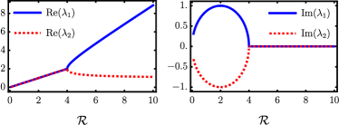
Figure 1: Real and imaginary parts of $\lambda_{1}$, and $\lambda_{2}$ defined in Eq. (14) for energies $\epsilon\simeq 0$ corresponding to surface eigenstates.

Then, by solving the linear system Eq. (LABEL:eq_Dirac_system), we obtain four independent solutions (for $\alpha=1,2$ and $\widetilde{z}=z/R_{0}$)

$$\varphi_{\pm}^{(\alpha,\uparrow)}(\widetilde{z},\epsilon) = e^{\pm\widetilde{\lambda}_{\alpha}\widetilde{z}}\left(1,0,\pm\mathrm{i}A_{\alpha},0\right)^{T},$$

$$\varphi_{\pm}^{(\alpha,\downarrow)}(\widetilde{z},\epsilon) = e^{\pm\widetilde{\lambda}_{\alpha}\widetilde{z}}\left(0,1,0,\mp\mathrm{i}A_{\alpha}\right)^{T},$$ (15)

where we defined the parameters

$$A_{\alpha}=\frac{\widetilde{\lambda}_{\alpha}}{1-\frac{s}{\mathcal{R}}\widetilde{\lambda}^{2}_{\alpha}+\epsilon}.$$ (16)

The exponential decay length in Eq. (15) is thus a non-linear function of the energy eigenvalues after Eq. (14). In particular, for $\mathcal{R}\gg 1$ after Eq. (14) it is clear that $\tilde{\lambda}_{\alpha}\sim\mathcal{R}/\sqrt{2}$, i.e. the exponential decay of the surface states from each side of the slab is approximately determined by the magnitude of this parameter. Concerning the materials we present in Table 1, realistic values are $\mathcal{R}=0.169$ for ${\rm{Bi}}_{2}{\rm{Se}}_{3}$ and $\mathcal{R}=0.021$ for ${\rm{Bi}}_{s}{\rm{Te}}_{3}$, respectively, and hence the imaginary part of the $\lambda_{1,2}$ does not vanish in both cases. Moreover, based on these material specific examples, we shall focus on the analysis for representative values $\mathcal{R}\leq 1$.

We remark that these independent solutions are trivially orthogonal for opposite spin components, i.e. (for $\beta,\,\beta^{\prime}=\pm$, $\alpha,\,\alpha^{\prime}=1,2$)

$$\langle\alpha\uparrow;\beta|\alpha^{\prime}\downarrow;\beta^{\prime}\rangle=\int_{0}^{\tilde{d}}d\tilde{z}\left[\varphi^{(\alpha,\uparrow)}_{\beta}(\tilde{z})\right]^{\dagger}\varphi^{(\alpha^{\prime},\downarrow)}_{\beta^{\prime}}(\tilde{z})=0,$$ (17)

while those with parallel spin components satisfy the inner product result

$$\langle\alpha\downarrow;\beta|\alpha^{\prime}\downarrow;\beta^{\prime}\rangle = \langle\alpha\uparrow;\beta|\alpha^{\prime}\uparrow;\beta^{\prime}\rangle$$ (18)

$$= \tilde{d}\left(1+\beta\beta^{\prime}A_{\alpha}A_{\alpha^{\prime}}\right)e^{\left(\beta\tilde{\lambda}_{\alpha}+\beta^{\prime}\tilde{\lambda}_{\alpha^{\prime}}\right)\tilde{d}/2}$$

$$\times\frac{\sinh\left[\left(\beta\tilde{\lambda}_{\alpha}+\beta^{\prime}\tilde{\lambda}_{\alpha^{\prime}}\right)\tilde{d}/2\right]}{\left(\beta\tilde{\lambda}_{\alpha}+\beta^{\prime}\tilde{\lambda}_{\alpha^{\prime}}\right)\tilde{d}/2}.$$

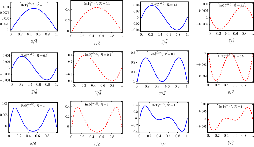
Figure 2: Real and imaginary parts of the surface eigenstate $\Psi_{\text{surf}}^{\uparrow}=\left[\Psi_{1}^{(\text{surf},\uparrow)},0,\Psi_{3}^{(\text{surf},\uparrow)},0\right]^{T}$, for different values of $\mathcal{R}$.

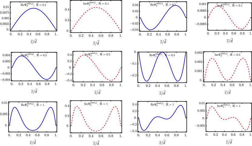
Figure 3: Real and imaginary parts of the surface eigenstate $\Psi_{\text{surf}}^{\downarrow}=\left[0,\Psi_{2}^{(\text{surf},\downarrow)},0,\Psi_{4}^{(\text{surf},\downarrow)}\right]^{T}$, for different values of $\mathcal{R}$.

Therefore, it is natural to define independent surface states for each fixed spin projection $\sigma=\uparrow$ or $\sigma=\downarrow$ as follows

$$\Psi_{\text{surface}}^{(\sigma)}(\widetilde{z})=\sum_{\alpha=1,2}\sum_{\beta=\pm}a_{\beta}^{(\alpha)}\varphi_{\beta}^{(\alpha,\sigma)}(\widetilde{z}),$$ (19)

where $a_{\beta}^{(\alpha)}$ represent arbitrary coefficients in the general linear combination. Those coefficients are further defined upon imposing, for each spin projection state $\sigma=\uparrow$ or $\sigma=\downarrow$, the boundary conditions at each surface of the slab,

$$\Psi_{\text{surface}}^{(\sigma)}(\widetilde{z}=0)=\Psi_{\text{surface}}^{(\sigma)}(\widetilde{z}=d/R_{0})=0.$$ (20)

Those lead to the secular linear system

$$\mathbb{A}~{}\bm{a}=0,$$ (21)

where $\bm{a}\equiv\left(a_{+}^{(1)},a_{-}^{(1)},a_{+}^{(2)},a_{-}^{(2)}\right)^{T}$ is the vector of coefficients, and the matrix $\mathbb{A}$ is defined as (for $\widetilde{d}\equiv d/R_{0}$)

$$\mathbb{A}\equiv\begin{pmatrix}1&1&1&1\\ \mathrm{i}A_{1}&-\mathrm{i}A_{1}&\mathrm{i}A_{2}&-\mathrm{i}A_{2}\\ e^{\widetilde{\lambda}_{1}\widetilde{d}}&e^{-\widetilde{\lambda}_{1}\widetilde{d}}&e^{\widetilde{\lambda}_{2}\widetilde{d}}&e^{-\widetilde{\lambda}_{2}\widetilde{d}}\\ \mathrm{i}A_{1}e^{\widetilde{\lambda}_{1}\widetilde{d}}&-\mathrm{i}A_{1}e^{-\widetilde{\lambda}_{1}\widetilde{d}}&\mathrm{i}A_{2}e^{\widetilde{\lambda}_{2}\widetilde{d}}&-\mathrm{i}A_{2}e^{-\widetilde{\lambda}_{2}\widetilde{d}}\end{pmatrix}.$$ (22)

The existence of non-trivial solutions for the coefficients $\bm{a}$ that satisfy the boundary conditions Eq. (20) is granted provided $\det\mathbb{A}=0$. This equation can be expressed in a closed algebraic form as

$$\frac{\widetilde{\lambda}_{1}}{\widetilde{\lambda}_{2}}\frac{1+\epsilon-\widetilde{\lambda}_{2}^{2}/\mathcal{R}}{1+\epsilon-\widetilde{\lambda}_{1}^{2}/\mathcal{R}}v(\widetilde{\lambda}_{1},\widetilde{\lambda}_{2})=u(\widetilde{\lambda}_{1},\widetilde{\lambda}_{2})$$

$$-\sqrt{u^{2}(\widetilde{\lambda}_{1},\widetilde{\lambda}_{2})-v^{2}(\widetilde{\lambda}_{1},\widetilde{\lambda}_{2})},$$ (23)

with the definitions $u(\widetilde{\lambda}_{1},\widetilde{\lambda}_{2})\equiv\cosh(\widetilde{d}~{}\widetilde{\lambda}_{1})\cosh(\widetilde{d}~{}\widetilde{\lambda}_{2})-1$ and $v(\widetilde{\lambda}_{1},\widetilde{\lambda}_{2})\equiv\sinh(\widetilde{d}~{}\widetilde{\lambda}_{1})\sinh(\widetilde{d}~{}\widetilde{\lambda}_{2})$, respectively.

Furthermore, from the first three rows of Eq. (21) we obtain

$$\bar{a}_{-}^{(1)} \equiv a_{-}^{(1)}/a_{+}^{(1)}=\frac{\left(e^{2\widetilde{d}~{}\widetilde{\lambda}_{2}}-1\right)e^{\widetilde{d}~{}\widetilde{\lambda}_{1}}A_{1}+\left(1+e^{2\widetilde{d}~{}\widetilde{\lambda}_{2}}-2e^{\widetilde{d}(\widetilde{\lambda}_{1}+\widetilde{\lambda}_{2})}\right)e^{\widetilde{d}~{}\widetilde{\lambda}_{1}}A_{2}}{e^{\widetilde{d}~{}\widetilde{\lambda}_{1}}\left(e^{2\widetilde{d}~{}\widetilde{\lambda}_{2}}-1\right)A_{1}-\left(e^{\widetilde{d}~{}\widetilde{\lambda}_{1}}-2e^{\widetilde{d}~{}\widetilde{\lambda}_{2}}+e^{\widetilde{d}(\widetilde{\lambda}_{1}+2\widetilde{\lambda}_{2})}\right)A_{2}}$$

$$\bar{a}_{+}^{(2)} \equiv a_{+}^{(2)}/a_{+}^{(1)}=\frac{\left(e^{2\widetilde{d}~{}\widetilde{\lambda}_{1}}-1\right)e^{\widetilde{d}~{}\widetilde{\lambda}_{2}}A_{2}-\left(e^{\widetilde{d}~{}\widetilde{\lambda}_{2}}-2e^{\widetilde{d}~{}\widetilde{\lambda}_{1}}+e^{\widetilde{d}(2\widetilde{\lambda}_{1}+\widetilde{\lambda}_{2})}\right)A_{1}}{e^{\widetilde{d}~{}\widetilde{\lambda}_{1}}\left(e^{2\widetilde{d}~{}\widetilde{\lambda}_{2}}-1\right)A_{1}-\left(e^{\widetilde{d}~{}\widetilde{\lambda}_{1}}-2e^{\widetilde{d}~{}\widetilde{\lambda}_{2}}+e^{\widetilde{d}(\widetilde{\lambda}_{1}+2\widetilde{\lambda}_{2})}\right)A_{2}}$$

$$\bar{a}_{-}^{(2)} \equiv a_{-}^{(2)}/a_{+}^{(1)}=\frac{\left(e^{2\widetilde{d}~{}\widetilde{\lambda}_{1}}-1\right)e^{\widetilde{d}~{}\widetilde{\lambda}_{1}}A_{2}+\left(1+e^{\widetilde{d}~{}\widetilde{\lambda}_{1}}-2e^{\widetilde{d}(\widetilde{\lambda}_{1}+\widetilde{\lambda}_{2})}\right)e^{\widetilde{d}~{}\widetilde{\lambda}_{1}}A_{1}}{e^{\widetilde{d}~{}\widetilde{\lambda}_{1}}\left(e^{2\widetilde{d}~{}\widetilde{\lambda}_{2}}-1\right)A_{1}-\left(e^{\widetilde{d}~{}\widetilde{\lambda}_{1}}-2e^{\widetilde{d}~{}\widetilde{\lambda}_{2}}+e^{\widetilde{d}(\widetilde{\lambda}_{1}+2\widetilde{\lambda}_{2})}\right)A_{2}}.$$ (24)

Note that the constants in Eq. (19) are the same for both spin projections, so we can finally write

$$\Psi_{\text{surface}}^{(\uparrow)}(\widetilde{z},\epsilon) = C_{\uparrow}\sum_{\alpha=1,2}\sum_{\beta=\pm}\bar{a}_{\beta}^{(\alpha)}\varphi_{\beta}^{(\alpha,\uparrow)}(\widetilde{z})$$

$$\Psi_{\text{surface}}^{(\downarrow)}(\widetilde{z}.\epsilon) = C_{\downarrow}\sum_{\alpha=1,2}\sum_{\beta=\pm}\bar{a}_{\beta}^{(\alpha)}\varphi_{\beta}^{(\alpha,\downarrow)}(\widetilde{z}).$$ (25)

Here, we defined $\bar{a}_{+}^{(1)}=1$, and the coefficients $C_{\uparrow}$, $C_{\downarrow}$ are determined by the normalization conditions as follows

$$|C_{\uparrow}| = \left[\sum_{\alpha=1,2}\sum_{\alpha^{\prime}=\pm}\sum_{\beta=1,2}\sum_{\beta^{\prime}=1,2}\bar{a}_{\beta}^{(\alpha)}\bar{a}_{\beta^{\prime}}^{(\alpha^{\prime})}\langle\alpha\uparrow;\beta|\alpha^{\prime}\uparrow;\beta^{\prime}\rangle\right]^{-1/2}$$

$$|C_{\downarrow}| = \left[\sum_{\alpha=1,2}\sum_{\alpha^{\prime}=\pm}\sum_{\beta=1,2}\sum_{\beta^{\prime}=1,2}\bar{a}_{\beta}^{(\alpha)}\bar{a}_{\beta^{\prime}}^{(\alpha^{\prime})}\langle\alpha\downarrow;\beta|\alpha^{\prime}\downarrow;\beta^{\prime}\rangle\right]^{-1/2},$$ (26)

where the analytical expression for the inner product coefficients are presented in Eq. (18). Moreover, from Eq. (17) it is clear that surface states with opposite spin components are mutually orthogonal

$$\langle\uparrow;\text{surface},\epsilon|\downarrow;\text{surface},\epsilon\rangle$$ (27)

$$= \int_{0}^{\tilde{d}}d\tilde{z}\left[\Psi_{\text{surface}}^{(\uparrow)}(\tilde{z},\epsilon)\right]^{\dagger}\Psi_{\text{surface}}^{(\downarrow)}(\tilde{z},\epsilon)=0.$$

The system of equations Eq. (14) and Eq. (23) must be solved in favor of $\epsilon$. By inspection, it is evident that a solution is found when

$$\widetilde{d}~{}\widetilde{\lambda}_{2}=0~{}~{}\text{and}~{}~{}\epsilon=-1$$ (28)

so that, this condition implies, after Eq. (14)

$$\widetilde{\lambda}_{1}=\mathcal{R}\left(1+\frac{2s}{\mathcal{R}}\right).$$ (29)

On the other hand, nontrivial solutions corresponding to true surface states can exist when $\epsilon\simeq 0$, and those can only be found numerically as a function of the system thickness $d$.

An important property of these surface states, determined from the numerical solutions of the algebraic system of equations detailed in this section, is the well-defined parity of their components with respect to the center of the slab at $z=d/2$, i.e.

$$\Psi^{(\text{surface},\sigma)}_{j}(d/2-\zeta,\epsilon)=(-1)^{P}\Psi^{(\text{surface},\sigma)}_{j}(d/2+\zeta,\epsilon)$$ (30)

where $j$ labels the component ($j=1,\ldots,4$), and $\zeta\in[-d/2,d/2]$ represents the distance from the center of the slab. Here, the parity index $P$ is odd ($P=1$) or even ($P=2$), depending on the spin polarization of the surface state and the magnitude of $\mathcal{R}$. As shown in Fig. 2, for the $\sigma=\uparrow$ spin polarization, the only non-vanishing components are $j=1,3$. When $\mathcal{R}=0.1$ and $\mathcal{R}=1$, the component $j=1$ has even parity $P=2$, while the $j=3$ component possesses odd parity $P=1$. In contrast, we observe that the parities are reversed when $\mathcal{R}=0.5$.

A similar behavior is observed in Fig. 3 for the $\sigma=\downarrow$ spin polarization, when in this case it is the $j=2$ and $j=4$ components which are non-zero and alternate their well defined but opposite parities as a function of $\mathcal{R}$.

Nevertheless, despite both components always have opposite parities, the corresponding probability density $\rho_{{\rm{surface}}}^{(\sigma)}(z)=\Psi_{{\rm{surface}}}^{\sigma\dagger}(z)\Psi_{{\rm{surface}}}^{\sigma}(z)$ for either spin polarization $\sigma$ remains symmetric with respect to the center of the slab

$$\rho_{{\rm{surface}}}^{(\sigma)}(d/2-\zeta)=\rho_{{\rm{surface}}}^{(\sigma)}(d/2+\zeta).$$ (31)

IV The bulk eigenstates

The bulk states are obtained from the same system of equations Eq. (LABEL:eq_Dirac_system), but with the $z$-component of momentum $\tilde{k}_{z}$ a real number. From Eq. (11), we have that the general solution is given by the linear combination of spinors

$$\Phi^{\pm}_{\text{bulk}}(z) = \begin{pmatrix}\eta_{\text{bulk}}^{\pm}\\ \\ \chi_{\text{bulk}}^{\pm}\end{pmatrix}$$ (32)

$$= ue^{\pm\mathrm{i}\tilde{k}_{z}\widetilde{z}}\begin{pmatrix}1\\ 0\\ B_{z}\\ 0\end{pmatrix}+ve^{\pm\mathrm{i}\tilde{k}_{z}\widetilde{z}}\begin{pmatrix}0\\ 1\\ 0\\ -B_{z}\end{pmatrix},$$

with

$$B_{z}=\frac{s\tilde{k}_{z}}{1+\frac{s}{\mathcal{R}}\tilde{k}_{z}^{2}+\epsilon_{\text{bulk}}}.$$ (33)

Now, by applying the confinement boundary conditions

$$\phi_{\text{bulk}}(\widetilde{z}=0)=\phi_{\text{bulk}}(\widetilde{z}=\tilde{d})=0,$$ (34)

we conclude that the appropriate linear combination (modulo a normalization constant) is

$$\phi_{\text{bulk}}(\widetilde{z})=\Phi^{+}_{\text{bulk}}(\widetilde{z})-\Phi^{-}_{\text{bulk}}(\widetilde{z})\propto\sin(\tilde{k}_{z}\widetilde{z}),$$ (35)

provided

$$\sin(\tilde{k}_{z}\tilde{d})=0,$$ (36)

which leads to the quantization condition for $\tilde{k}_{z}$

$$\widetilde{k}_{z}=\frac{n\pi}{\widetilde{d}},~{}\text{for}~{}n=\pm 1,\pm 2,\ldots$$ (37)

Therefore, from Eq. (13) the quantized energy eigenvalues due to spatial confinement in the region $0\leq z\leq d$ are given by

$$\epsilon_{\text{bulk}}^{2}=\frac{n^{2}\pi^{2}}{\widetilde{d}^{2}}+\left(1+\frac{s}{\mathcal{R}}\frac{n^{2}\pi^{2}}{\widetilde{d}^{2}}\right)^{2}.$$ (38)

The corresponding normalized bulk eigenstates for each spin projection are

$$\phi_{\text{bulk}}^{(n,\uparrow)}(\widetilde{z}) = \sqrt{\frac{2}{(1+B_{n}^{2})\tilde{d}}}\sin\left(\frac{n\pi\widetilde{z}}{\widetilde{d}}\right)\left(1,0,B_{n},0\right)^{T},$$

$$\phi_{\text{bulk}}^{(n,\downarrow)}(\widetilde{z}) = \sqrt{\frac{2}{(1+B_{n}^{2})\tilde{d}}}\sin\left(\frac{n\pi\widetilde{z}}{\widetilde{d}}\right)\left(0,1,0,-B_{n}\right)^{T},$$

with $\widetilde{d}\equiv d/R_{0}$, and the coefficients $B_{n}$ defined as

$$B_{n}=B_{z}\left(\tilde{k}_{z}=\frac{n\pi}{\widetilde{d}}\right)=\frac{sn\pi/\widetilde{d}}{1+\frac{s}{\mathcal{R}}\left(\frac{n\pi}{\widetilde{d}}\right)^{2}+\epsilon_{\text{bulk}}}.$$ (40)

The normalization constants are defined such that (for $\sigma=\uparrow,\downarrow$)

$$\int_{0}^{\tilde{d}}d\widetilde{z}\left[\phi_{\text{bulk}}^{n,\sigma}(\widetilde{z})\right]^{\dagger}\phi_{\text{bulk}}^{n,\sigma}(\widetilde{z})=1.$$ (41)

A noteworthy property of these spin projection eigenstates is their even/odd parity with respect to the center of the slab $z=d/2$, since for $\zeta\in[-d/2,d/2]$ the distance from the center of the slab, we have

$$\sin\left(\frac{n\pi}{d}\left(d/2-\zeta\right)\right)=(-1)^{n+1}\sin\left(\frac{n\pi}{d}\left(d/2+\zeta\right)\right).$$ (42)

Therefore, the same even/odd parity is inherited by the spinor functions

$$\phi_{\text{bulk}}^{n,\sigma}\left(d/2-\zeta\right)=(-1)^{n+1}\phi_{\text{bulk}}^{n,\sigma}\left(d/2+\zeta\right).$$ (43)

V Surface - bulk hybridization and the breaking of inversion symmetry

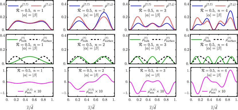
Figure 4: Electronic density distribution $\rho_{n,\epsilon}^{\sigma,\sigma^{\prime}}(\widetilde{z})$ and its independent surface $\rho_{\text{surface}}$, bulk $\rho_{\text{bulk}}$, and interference $\rho_{\text{mix}}$ components, respectively, as defined in Eq. (45) for the coupling between $(\sigma,\sigma^{\prime})=(\uparrow,\uparrow)$ and $(\uparrow,\downarrow)$. Note that if $\sigma\neq\sigma^{\prime}\to\rho_{\text{mix}}^{(\sigma,\sigma^{\prime})}=0$.

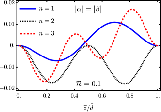
Figure 5: Behavior of $\rho_{\text{mix}}^{(\uparrow,\uparrow)}$ as a function of $\mathcal{R}$, and $n$.

As discussed in Eq. (30), depending on the magnitude of $\mathcal{R}$, the spinor components of the surface states possess well defined but opposite parities $P$ with respect to a mirror plane located at the center of the slab $z=d/2$. On the other hand, the bulk states exhibit a global parity determined by the number of nodes within the finite domain $z\in[0,d]$ imposed by the boundaries of the slab, which depends on the quantum number $n\geq 1$, as stated in Eq. (43).

Let us now consider the existence of a hybrid surface-bulk state described by the linear combination

$$\Psi_{n,\epsilon}^{\left(\sigma,\sigma^{\prime}\right)}(\widetilde{z})=\alpha\Psi^{(\sigma)}_{\text{surface}}(\widetilde{z},\epsilon)+\beta\phi_{\text{bulk}}^{(n,\sigma^{\prime})}(\widetilde{z}).$$ (44)

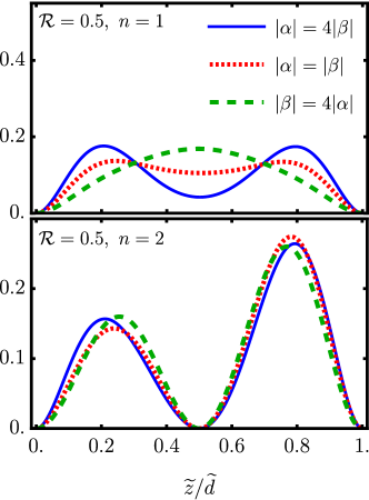
Figure 6: Spatial distribution of $\rho_{\rm{n,\epsilon}}^{(\uparrow,\uparrow)}(\tilde{z})$ for different coefficients $\alpha$ and $\beta$ in the hybrid state Eq. (44).

The probability distribution corresponding to this hybrid state is given by the expression

$$\rho^{(\sigma,\sigma^{\prime})}_{n,\epsilon}(z)=\rho_{\text{surface}}^{(\sigma)}(z)+\rho_{\text{bulk}}^{(\sigma^{\prime})}(z)+\rho_{\text{mix}}^{(\sigma,\sigma^{\prime})}(z),$$ (45)

where

$$\rho_{\text{mix}}^{(\sigma,\sigma^{\prime})}=2\text{Re}\left\{\alpha^{*}\beta\braket{\text{surface},\sigma}{\text{bulk},\sigma^{\prime}}\right\}$$ (46)

represents the contribution due to the quantum interference effect between surface and bulk in the hybrid state in Eq. (44). As a trivial consequence of Eq. (30) and Eq. (43), the probability density contributions $\rho_{\text{surface}}^{(\sigma)}(z)=|\alpha|^{2}|\Psi_{\text{surface}}^{(\sigma)}(z,\epsilon)|^{2}$ and $\rho_{\text{bulk}}^{(\sigma)}(z)=|\beta|^{2}|\phi_{\text{bulk}}^{(n,\sigma)}(z)|^{2}$ arising independently from surface and bulk, respectively, are symmetric with respect to the center of the slab, regardless of their spin or parity. This feature is clearly illustrated in the central row of the panel Fig. 4, by the solid (bulk) and dashed (surface) lines, respectively.

Clearly, for opposite spins $\sigma\neq\sigma^{\prime}$ the components of the surface and bulk spinor states are mutually orthogonal such that $\rho_{\text{mix}}^{(\sigma\neq\sigma^{\prime})}=0$, and hence the probability density is indeed trivially symmetric with respect to a mirror plane at the center of the slab $z=d/2$, i.e.

$$\rho_{n,\epsilon}^{(\sigma\neq\sigma^{\prime})}(d/2-\zeta)=\rho_{n,\epsilon}^{(\sigma\neq\sigma^{\prime})}(d/2+\zeta),$$ (47)

for $\zeta\in[-d/2,d/2]$ the distance from the center. This is clearly shown in the first row of the panel Fig. 4, where the dotted line represents the total probability density $\rho^{(\uparrow,\downarrow)}$ for opposite spin components in the hybrid state when $|\alpha|=|\beta|$ in the superposition Eq. (44).

In contrast, a very non-trivial behavior is observed when surface and bulk in the hybrid state Eq. (44) possess parallel spins ($\sigma=\sigma^{\prime}$). In this last case, the mixture term does not vanish, as illustrated in the bottom row of the panel Fig. 4, for the choice $|\alpha|=|\beta|$ in the combination of the hybrid state in Eq. (44). Interestingly, given that the surface spinor components possess alternate parities (see Eq. (30)), while the bulk spinor possesses a well defined global parity (see Eq. (43)), the mixture term $\rho_{{\rm{mix}}}^{(\sigma,\sigma)}$ does not exhibit, in general, a well defined parity for arbitrary values of $n$ and $\mathcal{R}$. However, as can be appreciated in Fig. 2 for $\sigma=\uparrow$ and Fig. 3 for $\sigma=\downarrow$, respectively, when $\mathcal{R}\lesssim 1$ we have that

$$\left|\text{Re}\Psi^{(\text{surface},\sigma)}_{j}\right|\ll\left|\text{Re}\Psi^{(\text{surface},\sigma)}_{j+2}\right|,$$ (48)

and in such case the mix term acquires an approximate symmetry imposed by the parity of the bulk state. This property of the mixture density term is appreciated in Fig. 5, for $\mathcal{R}=0.1$ and different values of $n$, the later determining the parity of the bulk state according to Eq. (43). In consequence, the mirror symmetry of the total probability density for the hybrid surface-bulk state defined by Eq. (45) may be broken for parallel spin components, depending on the combination of values of $\mathcal{R}$ and $n$. These occurrences are material-specific because $\mathcal{R}$ depends on the Compton decay length. Consequently, the subtleties of symmetry breaking remain distinctive for each material due to their unique characteristics. A graphical illustration of this effect is observed in the first row of the panel Fig. 4, where the solid line represents the total probability density $\rho^{(\uparrow,\uparrow)}$ for parallel spin components in the hybrid state when $|\alpha|=|\beta|$ in the superposition Eq. (44).

This rather counter-intuitive result, given the symmetric boundary conditions in the slab geometry, is clearly a pure quantum mechanical effect due to interference contained in the mixture term.

Figure 6 highlights the effect of the coefficients $\alpha$ and $\beta$ in the linear combination described by Eq. (44). The general considerations regarding inversion symmetry remain unaffected. As expected, larger values of $|\alpha|>|\beta|$ imply an increasingly important contribution from the surface state in the hybrid combination Eq. (44), and correspondingly the weight of the probability distribution is more concentrated towards the edges. Conversely, when $|\beta|>|\alpha|$ the probability density of the hybrid state displays more weight towards the bulk. A similar effect is observed as a function of $n$, since for $n\gg 1$, the hybrid state displays more statistical weight in the bulk.

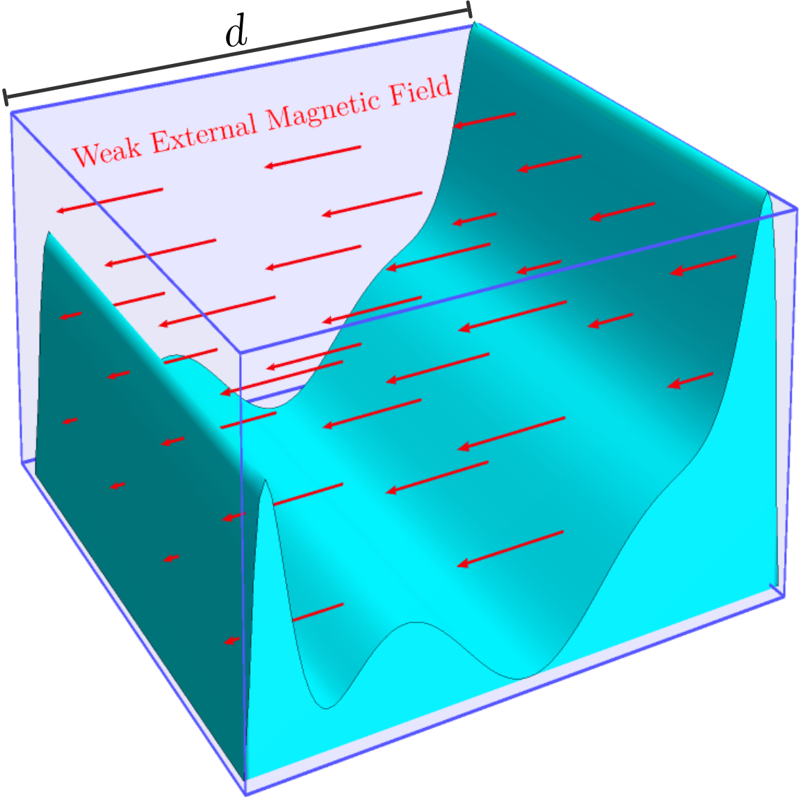
Figure 7: The geometrical configuration discussed in the model: A topological insulator (T.I.) slab of thickness $d$, subjected to a constant and weak magnetic field aligns the spins of surface and bulk electrons in the same direction. This alignment may result in an asymmetric probability density distribution, depicted by the cyan surface.

VI Conclusions

By means of a standard continuum effective model for a TI in a slab geometry, we explicitly obtained the surface and confined bulk states, in order to investigate the potential effects of their hybridization in the probability density, an important physical parameter that determines the electronic transport properties of such materials near the Fermi level. We assumed symmetric boundary conditions that consistently lead to probability density distributions for the bulk and surface states that possess a mirror symmetry with respect to a plane at the center of the slab. Surprisingly, our analytical and numerical results reveal that, when the spin components of surface and bulk in the hybrid state are parallel to each other, the symmetry in the probability density is spontaneously broken under certain conditions, depending on the combination of $n$ (the quantum number in the bulk solution) and the material-dependent parameter $\mathcal{R}$. We can explain this effect in simple terms, due to the spatially asymmetric interference pattern arising between surface and bulk, as captured in the $\rho_{{\text{mix}}}^{(\sigma,\sigma)}$ contribution for parallel spin components.

In this study, we are not delving into the detailed microscopic mechanism leading to the surface-bulk hybridization, which has been argued to be triggered, for instance, by disorder effects Saha and Garate (2014); Black-Schaffer and Balatsky (2012); Mandal et al. (2023); Yang et al. (2020); Hikami et al. (1980), or analyzed by means of a Fano model with a phenomenological coupling constant Hsu et al. (2014) in previous works. In contrast, we are here focusing on its possible consequences on the resulting probability density distribution. We found that under certain configurations, when the surface and bulk spin polarizations in the hybrid state are parallel, it may display an asymmetric probability density distribution, a theoretical result not previously reported in the literature Hsu et al. (2014); Saha and Garate (2014); Black-Schaffer and Balatsky (2012); Mandal et al. (2023); Yang et al. (2020); Hikami et al. (1980), even though the importance of spin polarization for the emergence of the surface state was already recognized by first-principles calculations in slab geometries Reid et al. (2020).

An experimental scenario where this interesting effect could be observed involves the presence of a constant, weak magnetic field $\mathbf{B}=\hat{z}B$ acting upon the topological insulator slab, as depicted in Fig. 7. In this scenario, the external field acts as a perturbation that does not alter the system’s ground state but breaks its spin degeneracy via the Zeeman coupling. This coupling, involving a magnetic moment $\mu$, results in a linear shift in the corresponding energy eigenvalues described by Eq. (9) as $\epsilon\to\epsilon-s\mu B/2$, where $s=-1$ denotes the $(\uparrow,\downarrow)$ state and $s=+1$ represents the $(\uparrow,\uparrow)$ state. Consequently, under this condition the system tends to favor a hybrid quantum state with parallel spin components for surface and bulk, where we anticipate the emergence of this novel phenomenon. Supporting experimental evidence for this conjecture is indeed presented in the literature Buchenau et al. (2017). For instance, a study on magnetotransport in Bi₂Se₃ nanoplate devices reveals that the proximity of a magnetic substrate to a surface channel disrupts the symmetry between the top and bottom electronic densities, resulting in the decoupling of the quantum Hall effects on each surface Buchenau et al. (2017).

Conflict of interest

The authors declare no conflict of interest.

Data availability statement

All data generated or analysed during this study are included in this published article. Any additional information is available from the corresponding author on reasonable request.

Keywords

Topological insulators, surface states, bulk states, surface-bulk hybridization, symmetry breaking, electronic density.

References

- Hasan and Kane (2010) M. Z. Hasan and C. L. Kane, “Colloquium: Topological insulators,” Rev. Mod. Phys. 82, 3045–3067 (2010).
- Fu and Kane (2008) Liang Fu and C. L. Kane, “Superconducting proximity effect and majorana fermions at the surface of a topological insulator,” Phys. Rev. Lett. 100, 096407 (2008).
- Moore (2010) Joel E Moore, “The birth of topological insulators,” Nature 464, 194–198 (2010).
- Castaño-Yepes and Muñoz (2022) Jorge David Castaño-Yepes and Enrique Muñoz, “The role of morphology on the emergence of topologically trivial surface states and selection rules in topological-insulator nano-particles,” Results Phys. 39, 105712 (2022).
- Imura et al. (2012) Ken-Ichiro Imura, Yukinori Yoshimura, Yositake Takane, and Takahiro Fukui, “Spherical topological insulator,” Phys. Rev. B 86, 235119 (2012).
- Tian et al. (2013) Mingliang Tian, Wei Ning, Zhe Qu, Haifeng Du, Jian Wang, and Yuheng Zhang, “Dual evidence of surface Dirac states in thin cylindrical topological insulator Bi2Te3 nanowires,” Sci. Rep. 3, 1–7 (2013).
- Governale et al. (2020) Michele Governale, Bibek Bhandari, Fabio Taddei, Ken-Ichiro Imura, and Ulrich Zülicke, “Finite-size effects in cylindrical topological insulators,” New Journal of Physics 22, 063042 (2020).
- Zhou et al. (2008) Bin Zhou, Hai-Zhou Lu, Rui-Lin Chu, Shun-Qing Shen, and Qian Niu, “Finite Size Effects on Helical Edge States in a Quantum Spin-Hall System,” Phys. Rev. Lett. 101, 246807 (2008).
- Lu et al. (2010) Hai-Zhou Lu, Wen-Yu Shan, Wang Yao, Qian Niu, and Shun-Qing Shen, “Massive dirac fermions and spin physics in an ultrathin film of topological insulator,” Phys. Rev. B 81, 115407 (2010).
- Saha and Garate (2014) Kush Saha and Ion Garate, “Theory of bulk-surface coupling in topological insulator films,” Phys. Rev. B 90, 245418 (2014).
- Black-Schaffer and Balatsky (2012) Annica M. Black-Schaffer and Alexander V. Balatsky, “Strong potential impurities on the surface of a topological insulator,” Phys. Rev. B 85, 121103 (2012).
- Mandal et al. (2023) Shoubhik Mandal, Debarghya Mallick, Yugandhar Bitla, R Ganesan, and P S Anil Kumar, “Bulk-surface coupling in dual topological insulator Bi1Te1 and Sb-doped Bi1Te1 single crystals via electron-phonon interaction,” J. Phys.: Condens. Matter 35, 285001 (2023).
- Yang et al. (2020) Xu Yang, Liang Luo, Chirag Vaswani, Xin Zhao, Yongxin Yao, Di Cheng, Zhaoyu Liu, Richard H. J. Kim, Xinyu Liu, Malgorzata Dobrowolska-Furdyna, Jacek K. Furdyna, Ilias E. Perakis, Caizhuang Wang, Kaiming Ho, and Jigang Wang, “Light control of surface–bulk coupling by terahertz vibrational coherence in a topological insulator,” npj Quantum Materials 5, 13 (2020).
- Checkelsky et al. (2011) J. G. Checkelsky, Y. S. Hor, R. J. Cava, and N. P. Ong, “Bulk band gap and surface state conduction observed in voltage-tuned crystals of the topological insulator ,” Phys. Rev. Lett. 106, 196801 (2011).
- Chiatti et al. (2016) Olivio Chiatti, Christian Riha, Dominic Lawrenz, Marco Busch, Srujana Dusari, Jaime Sánchez-Barriga, Anna Mogilatenko, Lada V Yashina, Sergio Valencia, Akin A Ünal, et al., “2D layered transport properties from topological insulator Bi2Se3 single crystals and micro flakes,” Sci. Rep. 6, 1–11 (2016).
- Liao et al. (2017) Jian Liao, Yunbo Ou, Haiwen Liu, Ke He, Xucun Ma, Qi-Kun Xue, and Yongqing Li, “Enhanced electron dephasing in three-dimensional topological insulators,” Nat. Commun. 8, 16071 (2017).
- Steinberg et al. (2011) H. Steinberg, J.-B. Laloë, V. Fatemi, J. S. Moodera, and P. Jarillo-Herrero, “Electrically tunable surface-to-bulk coherent coupling in topological insulator thin films,” Phys. Rev. B 84, 233101 (2011).
- Zhao et al. (2013) Yanfei Zhao, Cui-Zu Chang, Ying Jiang, Ashley DaSilva, Yi Sun, Huichao Wang, Ying Xing, Yong Wang, Ke He, Xucun Ma, et al., “Demonstration of surface transport in a hybrid Bi2Se3/Bi2Te3 heterostructure,” Sci. Rep. 3, 3060 (2013).
- Li et al. (2015) Zhaoguo Li, Ion Garate, Jian Pan, Xiangang Wan, Taishi Chen, Wei Ning, Xiaoou Zhang, Fengqi Song, Yuze Meng, Xiaochen Hong, Xuefeng Wang, Li Pi, Xinran Wang, Baigeng Wang, Shiyan Li, Mark A. Reed, Leonid Glazman, and Guanghou Wang, “Experimental evidence and control of the bulk-mediated intersurface coupling in topological insulator nanoribbons,” Phys. Rev. B 91, 041401 (2015).
- Rosenbach et al. (2022) Daniel Rosenbach, Kristof Moors, Abdur R. Jalil, Jonas Kölzer, Erik Zimmermann, Jürgen Schubert, Soraya Karimzadah, Gregor Mussler, Peter Schüffelgen, Detlev Grützmacher, Hans Lüth, and Thomas Schäpers, “Gate-induced decoupling of surface and bulk state properties in selectively-deposited Bi2Te3 nanoribbons,” SciPost Phys. Core 5, 017 (2022).
- Singh et al. (2017) Sourabh Singh, R K Gopal, Jit Sarkar, Atul Pandey, Bhavesh G Patel, and Chiranjib Mitra, “Linear magnetoresistance and surface to bulk coupling in topological insulator thin films,” J. Phys.: Condens. Matter 29, 505601 (2017).
- Hsu et al. (2014) Yi-Ting Hsu, Mark H. Fischer, Taylor L. Hughes, Kyungwha Park, and Eun-Ah Kim, “Effects of surface-bulk hybridization in three-dimensional topological metals,” Phys. Rev. B 89, 205438 (2014).
- Liu et al. (2010) Chao-Xing Liu, Xiao-Liang Qi, HaiJun Zhang, Xi Dai, Zhong Fang, and Shou-Cheng Zhang, “Model hamiltonian for topological insulators,” Phys. Rev. B 82, 045122 (2010).
- Zhang et al. (2009) H. Zhang, C.-X. Liu, X.-L. Qi, X. Dai, Z. Fang, and S.-C. Zhang, “Topological insulators in Bi2Se3, Bi2Te3 and Sb2Te3 with a single Dirac cone on the surface,” Nature Physics 5, 438 (2009).
- Reid et al. (2020) Thomas K. Reid, S. Pamir Alpay, Alexander V. Balatsky, and Sanjeev K. Nayak, “First-principles modeling of binary layered topological insulators: Structural optimization and exchange-correlation functionals,” Phys. Rev. B 101, 085140 (2020).
- Buchenau et al. (2017) Sören Buchenau, Philip Sergelius, Christoph Wiegand, Svenja Bäß ler, Robert Zierold, Ho Sun Shin, Michael Rübhausen, Johannes Gooth, and Kornelius Nielsch, “Symmetry breaking of the surface mediated quantum Hall Effect in Bi2Se3 nanoplates using Fe3O4 substrates,” 2D Mater. 4, 015044 (2017).
- Nechaev and Krasovskii (2016) I. A. Nechaev and E. E. Krasovskii, “Relativistic Hamiltonians for centrosymmetric topological insulators from ab initio wave functions,” Phys. Rev. B 94, 201410(R) (2016).
- Assaf et al. (2017) B. A. Assaf, T. Phuphachong, V. V. Volobuev, G. Bauer, B. Springholz, L.-A. Vaulchier, and Y. Guldner, “Magnetooptical determination of a topological index,” npj Quantum Materials 2, 26 (2017).
- Nakajima (1963) Seizo Nakajima, “The crystal structure of Bi2Te3 xSex,” Journal of Physics and Chemistry of Solids 24, 479–485 (1963).
- Hikami et al. (1980) Shinobu Hikami, Anatoly I. Larkin, and Yosuke Nagaoka, “Spin-Orbit Interaction and Magnetoresistance in the Two Dimensional Random System,” Prog. Theor. Phys. 63, 707–710 (1980).