UFIFT-QG-23-06

Don’t Throw the Baby Out with the Bath Water

R. P. Woodard^†

Department of Physics, University of Florida,
Gainesville, FL 32611, UNITED STATES

ABSTRACT

I stress the importance of retaining a healthy classical limit while we search for an ultraviolet completion to quantum gravity. A key problem with negative-norm quantizations of higher derivative Lagrangians is that their classical limits do not correspond to real-valued metrics evolving in a real-valued spacetime. I also demonstrate that no completion based on the flat spacetime background S-matrix can suffice by providing an explicit example of a theory with unit S-matrix which still shows interesting changes in single-particle kinematics and in the evolution of its background. I discuss the implications of these considerations for the program of Asymptotic Safety. Finally, I urge that some attention be given to the possibility that quantum general relativity might make sense if only we could go beyond conventional perturbation theory.

PACS numbers: 04.50.Kd, 95.35.+d, 98.62.-g

Dedicated to the memory of Stanley Deser: teacher, mentor, friend.

^† e-mail: woodard@phys.ufl.edu

1 A Thought-Provoking Question

What is wrong with proclaiming that we have solved the problem of quantum gravity, and the answer is the 1-dimensional simple harmonic oscillator?

$$H=\frac{p^{2}}{2m}+\frac{1}{2}m\omega^{2}q^{2}\;.$$ (1)

This is an exemplary quantum theory: all its states are normalizable, with positive energies and positive norms. Indeed, we can explicitly write down a complete set of energy eigenstates with $E_{n}=(n+\frac{1}{2})\hbar\omega$,

$$\psi_{n}(q)=\Bigl{[}\frac{m\omega}{\pi\hbar}\Bigr{]}^{\frac{1}{4}}\frac{(a^{\dagger})^{n}}{\sqrt{n!}}\exp\Bigl{[}-\frac{m\omega}{2\hbar}q^{2}\Bigr{]}\quad,\quad a^{\dagger}\equiv\sqrt{\frac{m\omega}{2\hbar}}\,\Bigl{(}q-\frac{\hbar}{m\omega}\frac{d}{dq}\Bigr{)}\;.$$ (2)

Of course there is one little problem: our theory of “quantum gravity” fails to describe the tides — or the solar system, or gravitational redshift, or the precession of the perihelion of Mercury, or the bending of starlight, or Shapiro delay, or gravitational lensing, or the spin-down of the binary pulsar, or the existence of gravitational radiation, or cosmology — or any of the other phenomena which are explained by classical general relativity.

We thereby come to an important realization: any proposal for “quantum gravity” had better represent the quantization of classical gravitation. Note also that the phenomena I have listed are not described by a gravitational S-matrix. All available data [1] indicate that their explanation derives instead from a local, generally coordinate invariant field theory of a real-valued metric which exists on a real-valued spacetime, with unobservably small quantum gravitational fluctuations at currently attainable energy scales. Any proposal for “quantum gravity” which fails to obey this Correspondence Principle amounts to throwing the baby out with the bath water.

I do not mean to imply that there are no quantum gravitational data. The simplest explanation of the primordial scalar power spectrum is as the gravitational response to quantum fluctuations in whatever matter field(s) drove primordial inflation at a scale as much as 55 orders of magnitude higher than the present day [2]. Something like $10^{7}$ pixels of data on this exist [3], with estimates as high as $10^{16}$ potentially recoverable from highly redshifted 21 centimeter radiation [4, 5, 6]. The tensor power spectrum [7] is also potentially observable, although it has yet to be resolved [8]. At the current level of sensitivity, both spectra can be explained as tree order effects in quantum general relativity. The full development of 21-cm cosmology may eventually permit 1-loop corrections to be resolved [9], but these would arise from the finite, nonlocal part of quantum general relativity regarded as a low energy effective field theory [10, 11, 12, 13, 14, 15]. There is no prospect of soon acquiring data which can resolve the ultraviolet completion of general relativity.

We should recall why people believe general relativity requires an ultraviolet completion. In $D=4$ spacetime dimensions the Lagrangian of the most general, invariant, metric theory of dimension four includes four terms,

$$\mathcal{L}=\frac{(R-2\Lambda)\sqrt{-g}}{16\pi G}+\frac{\alpha}{2}R^{2}\sqrt{-g}+\frac{\beta}{2}C^{\rho\sigma\mu\nu}C_{\rho\sigma\mu\nu}\sqrt{-g}\;,$$ (3)

where $R$ is the Ricci scalar and $C^{\rho\sigma\mu\nu}$ is the Weyl tensor. Kelly Stelle long ago proved that a certain quantization of this model is perturbatively renormalizable [16], provided all four terms are allowed. The first two terms comprise general relativity with a cosmological constant, and they not only allowed, but required in order to explain current data [1]. The Eddington ($R^{2}$) term is also permitted as long as its coefficient $\alpha$ is positive. Indeed, this term plays a crucial role in Starobinsky’s model of primordial inflation [17], which so far agrees with all data from the epoch of primordial inflation [18, 19, 8]. The problem is the Weyl ($C^{\rho\sigma\mu\nu}C_{\rho\sigma\mu\nu}$) term. No matter the sign of $\beta$, it gives rise to a massive spin two degree of freedom which renders the classical theory virulently unstable [20]. The problem of quantum gravity is that the Weyl term is not permitted, even though it is required for perturbative renormalizability [21, 22, 23, 24, 25, 26, 27, 28, 29, 30, 31, 32].

The Weyl counterterm would so neatly solve the problem of quantum gravity that there is a long history of attempts to rehabilitate it [33, 34, 35, 36, 37, 38, 39, 40, 41, 42, 43, 44, 45, 46, 47]. Many of these efforts involve modifications such as the Lee-Wick mechanism [48, 49, 50, 51] and PT-symmetric quantization [52, 53]. Section 2 explains that these violate the Correspondence Principle stated above. Much of the pro-Weyl argumentation is based on the assumption that quantum gravity can be defined by its perturbative S-matrix on flat space background. Section 3 presents a nonlinear sigma model whose S-matrix is unity but which still shows interesting changes in both its background and in the spectrum of single particle states. Section 4 discusses why we really want a theory of quantum gravity, and the possibility that it might be nothing more than quantum general relativity. My conclusions comprise Section 5, which include comments on the consequences of the Correspondence Principle for the program of Asymptotic Safety [54, 55, 56].

2 Why the Weyl Counterterm Is Forbidden

There are really three points to make here. The first is that any local, invariant, metric extension of general relativity, except for $f(R)$ gravity, endows the classical theory with a virulent kinetic instability. Second, the quantization which was employed in Stelle’s proof [16] amounts to regarding the negative energy creation operators of (3) as positive energy annihilation operators. The resulting Fock “states” have positive energy but some of them have negative norm. These “states” are not normalizable under canonical quantization, but might be so in some alternate quantization scheme. However, and third, the classical limit of the resulting theory cannot be any local, invariant, metric theory of gravitation.

2.1 Why the Classical Theory Is Unstable

The fundamental problem of higher derivatives has nothing to do with gravity, or even field theory, so I will review it in the context of a point particle whose position is $q(t)$. Suppose the Lagrangian $L(q,\dot{q},\ddot{q})$ contains not just first derivatives $\dot{q}$ but also second derivatives $\ddot{q}$. Suppose also that it is nondegenerate, meaning that $\frac{\partial L}{\partial\ddot{q}}$ is monotonic in $\ddot{q}$. Ostrogradsky long ago showed that the canonical formalism of such a theory requires two coordinates and two momenta [57, 58],

$$Q_{1}\equiv q\qquad \qquad P_{1}\equiv\frac{\partial L}{\dot{q}}-\frac{d}{dt}\frac{\partial L}{\partial\ddot{q}}\;,\qquad$$ , (4)

$$Q_{2}\equiv\dot{q}\qquad \qquad P_{2}\equiv\frac{\partial L}{\partial\ddot{q}}\;.\qquad$$ , (5)

Note that the assumption of nondegeneracy means we can solve for $\ddot{q}$ as some function $a(Q_{1},Q_{2},P_{2})$, without involving $P_{1}$. Ostrogradsky’s Hamiltonian is,

$$H\Bigl{(}Q_{1},Q_{2},P_{1},P_{2}\Bigr{)}\equiv Q_{2}P_{1}+a\Bigl{(}Q_{1},Q_{2},P_{2}\Bigr{)}P_{2}-L\Bigl{(}Q_{1},Q_{2},a(Q_{1},Q_{2},P_{2})\Bigr{)}\;.$$ (6)

One can easily show that the canonical evolution equations just reproduce the definitions (4-5) and the Euler-Lagrange equation [58],

$$\dot{Q}_{i}=\frac{\partial H}{\partial P_{i}}\qquad,\qquad\dot{P}_{i}=-\frac{\partial H}{\partial Q_{i}}\;.$$ (7)

There are a number of things to note about Ostrogradsky’s Hamiltonian (6). First, because it is linear in the independent canonical coordinate $P_{1}$, $H$ can never be bounded, either below or above. Second, adding more higher derivatives just makes the problem worse: if the Lagrangian contains up to $N$ derivatives of $q$, and is nondegenerate in the highest one, then there will be $N$ canonical coordinates $Q_{i}$ and the Hamiltonian will be linear in $(N-1)$ of their conjugate momenta $P_{i}$. Third, this problem is very general, completely independent of any approximation technique such as perturbation theory. As long as there are nondegenerate higher derivatives, the Hamiltonian cannot be bounded. This is the most compelling explanation for why Newton’s assumption about physics being defined by second order equations of motion has not been contradicted in 336 years since the Principia.

We can now understand why the only permitted extension of general relativity is $f(R)$ models. Note first that adding a nondegenerate higher derivative makes the Hamiltonian linear in the new conjugate momentum which results. This means it is unbounded below, but also unbounded above. The usual case is that the Hamiltonian of the lower derivative theory was bounded below, so the new higher derivative degree of freedom is negative to make the higher derivative Hamiltonian unbounded below. But if the lower derivative theory was already negative energy then the new, higher derivative degree of freedom would be positive energy. That is exactly what happens for nonlinear functions of the Ricci scalar because the only higher time derivative in $R$ is of $h\equiv\ln[{\rm det}(g_{ij})]$,

$$R=-g^{00}\ddot{h}+f\Bigl{(}g,\partial g,\partial_{i}\dot{g}\Bigr{)}\;.$$ (8)

This degree of freedom corresponds to the Newtonian potential, and it would indeed destabilize general relativity were it not for the Hamiltonian constraint. So we get a positive energy degree of freedom when the Lagrangian depends nonlinearly on $R$. However, unconstrained negative energy degrees of freedom arise from more general contractions of the Riemann tensor, or from derivatives of $R$ [59].

Before closing I should comment on some misconceptions:

• The Ostrogradsky problem is a kinetic energy instability, not a potential energy one, so it manifests from the dynamical variable being driven towards wild time dependence, not some particular value.

• Negative energy states are no problem unless there are interactions which allow balancing positive and negative energy excitations.

• The really crippling instability is driven by the infinite entropy of the high momentum phase space of an interacting continuum field theory. Indeed, the only way to get a finite decay rate in this case is by artificially cutting off the integration over possible momenta [60]. On the other hand, stable higher derivative theories with a finite number of discrete degrees of freedom can exist [61].

• The problem is not that the energy decays to negative infinity — the energy of any solution is conserved. It is rather that solutions develop a wild time dependence as more and more positive and balancing negative energy degrees of freedom are excited. This is why a global constraint on the energy does no good [62]. What one needs instead is a constraint on the local negative degrees of freedom, such as the Hamiltonian constraint which controls the Newtonian potential.

• Continuum negative energy particles with a high mass do not decouple from low energy physics. Rather they couple more strongly because there are more ways to produce them, and balance energy by producing positive energy particles.

• The Ostrogradskian instability must survive canonical quantization because it afflicts a large part of the classical phase space.

2.2 How the Quantum Theory Got Negative Norms

I have just commented that the Ostrogradskian instability must survive canonical quantization. Yet the higher derivative gravity theory in Stelle’s theorem has no negative energy states [16]. Even more surprising, it does have negative norm states, which of course violates the probabilistic interpretation of quantum mechanics. How did this happen? The answer is that Stelle employed a noncanonical quantization, and he was right to do so because it is only this formulation of (3) which leads to a renormalizable theory.

To understand what happened it is useful to work in the context of a quadratic, higher derivative oscillator,

$$L=\frac{m}{2\omega^{2}}\Bigl{[}-g\ddot{q}^{2}+\omega^{2}\dot{q}^{2}-\omega^{4}q^{2}\Bigr{]}\;.$$ (9)

The general (classical and quantum) solution is a sum of two oscillators,

$$q(t)=\sum_{\lambda=\pm}\Bigl{[}C_{\lambda}\cos(k_{\lambda}t)+S_{\lambda}\sin(k_{\lambda}t)\Bigr{]}\qquad,\qquad k_{\pm}\equiv\omega\Bigl{[}\frac{1\!\mp\!\sqrt{1\!-\!4g}}{2g}\Bigr{]}^{\frac{1}{2}}\;,$$ (10)

where the canonical coordinate expressions for the coefficients are,

$$C_{\pm}\equiv\frac{\pm g}{\sqrt{1\!-\!4g}}\Bigl{[}\frac{k^{2}_{\mp}Q_{1}}{\omega^{2}}-\frac{P_{2}}{gm}\Bigr{]}\qquad,\qquad S_{\pm}\equiv\frac{\pm g}{\sqrt{1\!-\!4g}}\Bigl{[}\frac{P_{1}}{gmk_{\pm}}-\frac{k_{\pm}Q_{2}}{\omega^{2}}\Bigr{]}\;.$$ (11)

The Hamiltonian reveals that the $k_{+}$ mode carries positive energy while the $k_{-}$ mode is negative energy,

$$H=\frac{m}{2}\sqrt{1\!-\!4g}\Bigl{[}k_{+}^{2}\Bigl{(}C_{+}^{2}\!+\!S_{+}^{2}\Bigr{)}-k_{-}^{2}\Bigl{(}C_{-}^{2}\!+\!S_{-}^{2}\Bigr{)}\Bigr{]}\;.$$ (12)

The associated lowering operators are,

$$A_{\pm}=\sqrt{\frac{mk_{\pm}\sqrt{1\!-\!4g}}{2\hbar}}\Bigl{[}C_{\pm}\pm iS_{\pm}\Bigr{]}\;.$$ (13)

Writing the operators in the position representation $Q_{i}=q_{i}$ and $P_{i}=-i\hbar\frac{\partial}{\partial q_{i}}$ allows us to find the normalizable wave function they annihilate,

$$\Omega(q_{1},q_{2})=N\exp\Bigl{[}-\frac{mg}{2\hbar\omega^{2}}\Bigl{(}(k_{-}\!-\!k_{+})k_{+}k_{-}q_{1}^{2}-2ik_{+}k_{-}q_{1}q_{2}+(k_{-}\!-\!k_{+})q_{2}^{2}\Bigr{)}\Bigr{]}\;.$$ (14)

Just like any harmonic oscillator (1-2), we can define a complete set of energy eigenstates $H|N_{+},N_{-}\rangle=\hbar(N_{+}k_{+}-N_{-}k_{-})|N_{+},N_{-}\rangle$,

$$\Bigl{|}N_{+},N_{-}\Bigr{\rangle}\equiv\frac{(A_{+}^{\dagger})^{N_{+}}(A_{-}^{\dagger})^{N_{-}}}{\sqrt{N_{+}!\,N_{-}!}}\Bigl{|}\Omega\Bigr{\rangle}\qquad\Longrightarrow\qquad\Bigl{\langle}k,\ell\Bigl{|}k^{\prime},\ell^{\prime}\Bigr{\rangle}=\delta_{kk^{\prime}}\delta_{\ell\ell^{\prime}}\;.$$ (15)

This is the canonical formulation of (9), and it has negative energies (just like the classical theory) and positive norms. It also “makes sense” in that the expectation values of positive operators are positive,

$$\Bigl{\langle}\Omega\Bigl{|}q^{2}\Bigr{|}\Omega\Bigr{\rangle}=\frac{\hbar}{2m\sqrt{g}}\frac{1}{k_{-}\!-\!k_{+}}\qquad,\qquad\Bigl{\langle}\Omega\Bigl{|}\dot{q}^{2}\Bigr{|}\Omega\Bigr{\rangle}=\frac{\hbar\omega^{2}}{2mg}\frac{1}{k_{-}\!-\!k_{+}}\;.$$ (16)

This theory consists of a real-valued position evolving in real-valued time.

Stelle’s quantization was based on regarding the negative energy creation operator $A_{-}^{\dagger}$ as a positive energy annihilation operator. We can easily construct the state wave function $\overline{\Omega}(q_{1},q_{2})$ which is annihilated by $A_{+}$ and $A_{-}^{\dagger}$,

$$\overline{\Omega}(q_{1},q_{2})\propto\exp\Bigl{[}-\frac{mg}{2\hbar\omega^{2}}\Bigl{(}(k_{+}\!+\!k_{-})k_{+}k_{-}q_{1}^{2}+2ik_{+}k_{-}q_{1}q_{2}-(k_{+}\!+\!k_{-})q_{2}^{2}\Bigr{)}\Bigr{]}\;.$$ (17)

I have not given the normalization factor because this wave function is not normalizable. It is possible to define a set of energy eigenfunctions $H|\overline{N_{+},N_{-}}\rangle=\hbar(N_{+}k_{+}+N_{-}k_{-})|\overline{N_{+},N_{-}}\rangle$ analogous to (15),

$$\Bigl{|}\overline{N_{+},N_{-}}\Bigr{\rangle}\equiv\frac{(A_{+}^{\dagger})^{N_{+}}(A_{-})^{N_{-}}}{\sqrt{N_{+}!\,N_{-}!}}\Bigl{|}\overline{\Omega}\Bigr{\rangle}\;\Longrightarrow\;\Bigl{\langle}\overline{k,\ell}\Bigl{|}\overline{k^{\prime},\ell^{\prime}}\Bigr{\rangle}=(-1)^{\ell}\delta_{kk^{\prime}}\delta_{\ell\ell^{\prime}}\Bigl{\langle}\overline{\Omega}\Bigl{|}\overline{\Omega}\Bigr{\rangle}\;.$$ (18)

All of these eigenfunctions have positive energy, but the ones with odd $N_{-}$ have a negative norm. This shows up in the expectation value of the square of the velocity being negative,

$$\Bigl{\langle}\overline{\Omega}\Bigl{|}q^{2}\Bigr{|}\overline{\Omega}\Bigr{\rangle}=\frac{\hbar}{2m\sqrt{g}}\frac{\langle\overline{\Omega}|\overline{\Omega}\rangle}{k_{-}\!+\!k_{+}}\qquad,\qquad\Bigl{\langle}\overline{\Omega}\Bigl{|}\dot{q}^{2}\Bigr{|}\overline{\Omega}\Bigr{\rangle}=-\frac{\hbar\omega^{2}}{2mg}\frac{\langle\overline{\Omega}|\overline{\Omega}\rangle}{k_{-}\!+\!k_{+}}\;.$$ (19)

It is obvious from the negative sign on the velocity that this theory does not correspond to a real-valued position moving in real-valued time.

These sorts of eccentricities are standard in noncanonical quantization schemes [63, 64, 65]. Note that they have nothing per se to do with higher derivatives. One could just as easily get a purely negative energy set of eigenstates for the simple harmonic oscillator (1) by regarding the creation operator as an annihilation operator. Indeed, because the Schrödinger equation $H\psi(q)=E\psi(q)$ is a second order, ordinary differential equation, there are two linearly independent solutions for any energy: positive, negative, imaginary, etc. Normalizability puts the quantum in quantum mechanics.

Stelle is a good physicist and he understood all of this. The reason he quantized (3) the way he did is that perturbative renormalizability requires propagators to fall off like the inverse fourth power of the Euclidean momentum. To understand this, compare the propagator of the canonical theory,

$$i\Delta(t;t^{\prime})\equiv\Bigl{\langle}\Omega\Bigl{|}T\Bigl{[}q(t)q(t^{\prime})\Bigr{]}\Bigr{|}\Omega\Bigr{\rangle}=\frac{\hbar}{m\sqrt{1\!-\!4g}}\Bigl{\{}\frac{e^{-ik_{+}|t-t^{\prime}|}}{2k_{+}}+\frac{e^{ik_{-}|t-t^{\prime}|}}{2k_{-}}\Bigr{\}}\;,$$ (20)

with the propagator of noncanonically quantized theory,

$$i\overline{\Delta}(t;t^{\prime})\equiv\Bigl{\langle}\overline{\Omega}\Bigl{|}T\Bigl{[}q(t)q(t^{\prime})\Bigr{]}\Bigr{|}\overline{\Omega}\Bigr{\rangle}=\frac{\hbar}{m\sqrt{1\!-\!4g}}\Bigl{\{}\frac{e^{-ik_{+}|t-t^{\prime}|}}{2k_{+}}-\frac{e^{-ik_{-}|t-t^{\prime}|}}{2k_{-}}\Bigr{\}}\;.$$ (21)

One can express both as integrals over a dummy $0$-component momentum $k_{0}$ using the identity,

$$\int_{-\infty}^{\infty}\!\!\frac{dk_{0}}{2\pi}\frac{ie^{-ik_{0}(t-t^{\prime})}}{k_{0}^{2}\!-\!k^{2}\!+\!i\epsilon}=\frac{e^{-ik|t-t^{\prime}|}}{2k}\;.$$ (22)

The result for the canonical propagator (20) is,

$$i\Delta(t;t^{\prime})=-\frac{\hbar\omega^{2}}{mg}\int_{-\infty}^{\infty}\!\!\frac{dk_{0}}{2\pi}\frac{ie^{-ik_{0}(t-t^{\prime})}}{(k_{0}^{2}\!-\!k_{+}^{2}\!+\!i\epsilon)(k_{0}^{2}\!-\!k_{-}^{2}\!-\!i\epsilon)}\;.$$ (23)

The problem is that Euclideanization requires the $k_{0}$ contour to be Wick rotated into the 1st and 3rd quadrants, which will give residues from the factor $(k_{0}^{2}-k_{-}^{2}-i\epsilon)$,

$$-\frac{\hbar\omega^{2}}{mg}\frac{i}{(k_{0}^{2}\!-\!k_{+}^{2}\!+\!i\epsilon)(k_{0}^{2}\!-\!k_{-}^{2}\!-\!i\epsilon)}$$ (24)

$$\hskip 99.58464pt\longrightarrow-\frac{\hbar\omega^{2}}{mg}\frac{1}{(k_{E}^{2}\!+\!k_{+}^{2})(k_{E}^{2}\!+\!k_{-}^{2})}+\frac{2\pi\hbar\delta(k_{E}^{2}\!-\!k^{2}_{-})}{m\sqrt{1\!-\!4g}}\;.\qquad$$

In a $3+1$ dimensional field theory the residue terms only fall off like an energy delta function divided by a single power of the 3-momentum. The advantage of the noncanonical propagator (21) is that it avoids these residues,

$$i\overline{\Delta}(t;t^{\prime})=-\frac{\hbar\omega^{2}}{mg}\int_{-\infty}^{\infty}\!\!\frac{dk_{0}}{2\pi}\frac{ie^{-ik_{0}(t-t^{\prime})}}{(k_{0}^{2}\!-\!k_{+}^{2}\!+\!i\epsilon)(k_{0}^{2}\!-\!k_{-}^{2}\!+\!i\epsilon)}\;.$$ (25)

2.3 Why This Is Bad

The problem with the negative-norm quantization of higher derivative gravity (3) is that it violates the Correspondence Principle defined in section 1. The classical limit of this quantization cannot represent a local, invariant theory of a real-valued metric existing on a real-valued spacetime. Before discussing how bad this is, please take note of the fact that no amount of further tinkering with quantum higher derivative theory can avoid it. The fatal minus signs are required for the quantum theory to be renormalizable. We also have a complete catalog of local, invariant theories of a real-valued metric existing on a real-valued spacetime and none of them possess the properties asserted for the quantum higher derivative theory.

The test of any physical theory comes in its ability to explain and predict experiment and observation. I do not rule out the possibility that some alternate quantization of a classically unstable Lagrangian might do that. For example, the negative norm quantization of the quadratic model (9) cannot represent the position of a point particle evolving in real time, but that might not pose a problem if we have no sense of being able to measure such a particle. The problem for gravity is that, once coordinates are fixed, we do have a strong sense of being able to measure a real-valued metric existing on a real-valued spacetime. Abandoning canonical quantization for gravity puts everything that we know about classical, and even semi-classical, gravitation at risk — which is everything we know about gravity. It amounts to throwing the baby out with the bath water.

I want to stress again that the most stringent test of noncanonical quantization is not producing a satisfactory quantum theory. This article began by exhibiting an absurd theory of “quantum gravity” (1-2) which is completely consistent, so there never was any doubt that a satisfactory quantum theory could be defined. The real test is whether or not the resulting “quantum gravity” theory recovers the vast array of phenomena which are explained by classical gravitation, including the data on primordial perturbations which follow from semi-classical gravitation. Passing this test is automatic for canonical quantization but it is highly problematic when alternate quantizations are employed. And the burden of proof rests with the people who seek to rehabilitate the Weyl counterterm. Many of the rehabilitators are my friends, who have spent as many years as I have in trying to understand quantum gravity. I hope they will forgive me if I address them as “you” in discussing some of the arguments they make that their formulations of quantum gravity have satisfactory classical limits.

I often hear rehabilitators claim that recovering general relativity is guaranteed because their low energy perturbative S-matrix is approximately that of quantum general relativity. There are a number of problems with this view, starting with its reliance on the perturbative S-matrix. With the possible exception of the bending of starlight, known gravitational phenomena are not explained using perturbative scattering theory but rather a local field theory of a real-valued metric existing on a real-valued spacetime, and often responding to nonperturbatively strong sources such as neutron stars. I want to see this field theory, and I want to see the exact formulation of it, not what you think is a good approximation. By your own admission, you must add something to the S-matrix amplitudes of quantum general relativity to improve their behavior at high energies; I want to see the local field theory behind the addition, no matter how minor you believe it is.

Another common argument is that the classical theory is that of a real-valued metric on a real-valued spacetime whose Lagrangian is (3). That is not true. As explained in section 2.1, the classical theory is subject to a virulent kinetic instability whose lifetime is zero. You claim that your alternate quantization produces a theory with only positive energies, and that this is true for every value of $\hbar$, no matter how small. Hence the classical limit of your theory is not that of a real-valued metric on a real-valued spacetime whose Lagrangian is (3). Please tell me what it is.

I often hear it asserted that the negative norms only affect very short wavelength modes, about which we know nothing. This argument ignores the distinction between time and space. The negative norm quantization of (3) results in negative norm modes of high mass, which implies mode functions with high frequencies, but says nothing about the wave number. In fact, the negative norm Fourier mode sum includes macroscopic wave lengths, the same way that the positive norm mode sum does. One consequence is that the square of the time derivative of the invariant length between spacelike separated points ($[\int\dot{g}_{ij}dx^{i}dx^{j}]^{2}$) is negative, even for macroscopic separations, the same way that $\dot{q}^{2}$ is negative in expression (19). This is not acceptable.

Finally, I have heard it claimed that the classical limit of quantum gravity is as completely misleading as the classical limit of quantum chromodynamics. I’m sure the statement was not meant this way, but it sounds like an admission that my objections to noncanonical quantization schemes for gravity are valid. I stress again that everything we know about gravity is either classical or, in the case of primordial perturbations, semi-classical. If this is not recovered by your theory of “quantum gravity” then you have indeed thrown the baby out with the bath water.

3 Objections to S-Matrix Chauvinism

Those who seek to rehabilitate the Weyl counterterm often adopt what I call S-Matrix Chauvinism, which asserts that the perturbative S-matrix on flat space background defines physics and is all we can ever know. Believers refuse to consider quasi-local fields such as $\int\dot{g}_{ij}dx^{i}dx^{j}$, whose square is negative, even over macroscopic spacelike separations in the negative norm quantization of (3). To them, no problem is real unless it appears in the S-matrix. Scattering into negative norm states does not trouble them because these states are unstable, so they cannot really be present in the asymptotic scattering space. With some inspired tinkering such as the Lee-Wick mechanism, it seems reasonable to them that a unitary and causal scattering theory can be defined between positive norm and positive energy particles. Hope springs eternal. While not denying the utility of the S-matrix, I do dispute the extreme position that local fields have no meaning, and also the assertion that the S-matrix suffices to define physics.

3.1 Abandoning Local Fields Is Not Necessary

One of my current teaching assignments is graduate electrodynamics. It’s a fun course on what has to be the greatest story every told in physics: how men of genius pieced together mankind’s first relativistic, unified field theory. I use the classic text by the late J. D. Jackson [66] which takes the reader through a bewildering variety of different solutions for electric and magnetic fields. No one questions the validity of solving for these fields, or what the solutions mean. Yet we are told that it all becomes meaningless nonsense as soon as quantum effects are turned on, no matter how small they are. For example, quantum gravity makes a fractional correction of about $10^{-45}$ to the Coulomb potential of an electron at the Compton radius. The best human technology cannot measure an effect so small, yet we are told that it being anything other than zero means we must abandon local fields and base physics entirely on the S-matrix. That never made any sense to me.

The alleged incompatibility of quantum effects and local fields is certainly not for lack of a quantum generalization of the classical Maxwell equation. The required generalization is based on the evocatively named “vacuum polarization” $i[\mbox{}^{\mu}\Pi^{\nu}](x;x^{\prime})$, which is the 1PI 2-point function of the photon,

$$\partial_{\nu}F^{\nu\mu}(x)+\int d^{4}x^{\prime}\Bigl{[}\mbox{}^{\mu}\Pi^{\nu}\Bigr{]}(x;x^{\prime})A_{\nu}(x^{\prime})=J^{\mu}(x)\;.$$ (26)

Here $F_{\mu\nu}\equiv\partial_{\mu}A_{\nu}-\partial_{\nu}A_{\mu}$ is the field strength tensor and $J^{\mu}(x)$ is the current density. S-matrix chauvinists disparage this equation for three reasons:

• $[\mbox{}^{\mu}\Pi^{\nu}](x;x^{\prime})$ is not real;

• $[\mbox{}^{\mu}\Pi^{\nu}](x;x^{\prime})$ is nonzero for $x^{\prime\mu}$ outside the past light-cone of $x^{\mu}$; and

• The $[\mbox{}^{\mu}\Pi^{\nu}](x;x^{\prime})$ induced by quantum gravity is highly gauge dependent.

All three of these problems occur in the dimensionally regulated, primitive contribution from a single loop of gravitons on flat space background [67],

$$i\Bigl{[}\mbox{}^{\mu}\Pi^{\nu}\Bigr{]}(x;x^{\prime})=-\frac{\kappa^{2}\mathcal{C}_{0}(D,a,b)(D\!-\!2)\Gamma^{2}(\frac{D}{2}\!-\!1)}{32(D\!-\!1)\pi^{D}}\Bigl{[}\eta^{\mu\nu}\partial^{2}-\partial^{\mu}\partial^{\nu}\Bigr{]}\frac{1}{\Delta x^{2D-2}}\;.$$ (27)

Here $\kappa^{2}\equiv 8\pi\hbar G/c^{3}$ is the loop-counting parameter of quantum gravity, the Lorentz interval is,

$$\Delta x^{2}\equiv\Bigl{\|}\vec{x}-\vec{x}^{\prime}\Bigr{\|}^{2}-\Bigl{(}c|t-t^{\prime}|-i\epsilon\Bigr{)}^{2}\;,$$ (28)

and the dependence on the two covariant gauge parameters $a$ and $b$ is,

$$\mathcal{C}_{0}(a,b,D)=8+\frac{12(a\!-\!1)-24(b\!-\!1)^{2}}{(b\!-\!2)^{2}}+O(D\!-\!4)\;.$$ (29)

The first two problems derive from the vacuum polarization of expression (27) being an in-out matrix element appropriate to asymptotic scattering theory. Using it in the effective field equation (26) gives the in-out matrix element of $F_{\mu\nu}$, which is not necessarily real, even if the field operator is Hermitian, because the in and out vacua might differ. In 1960 Julian Schwinger devised a diagrammatic procedure [68, 69, 70, 71, 72, 73] for computing true expectation values which is almost as easy to use as the Feynman rules are for computing in-out matrix elements. When the associated vacuum polarization is employed in equation (26) the resulting solutions are real, and the only contributions from the integration over $x^{\prime\mu}$ are on or inside the past light-cone of $x^{\mu}$ [74, 75]. Further, it is very simple to convert the in-out vacuum polarization to the in-in one [76].

That leaves only the gauge problem. One can see from expression (29) that by taking the parameter $b$ close to two and varying the parameter $a$, we can make the quantum correction run all the way from minus infinity to plus infinity. This is clearly unacceptable. It is also the result of a mistake. The effective field must be excited by some physical source, and it must be detected by some physical observer. The source and observer interact with gravity because all things do. Ignoring the resulting quantum gravitational correlations is what causes the gauge dependence of the effective field equation [77]. When proper account is taken of these correlations the renormalized result is a completely gauge independent effective field equation which is manifestly real and causal [78],

$$\partial_{\nu}F^{\nu\mu}(x)+\frac{5\hbar G\partial^{6}}{48\pi^{2}c^{3}}$$ (30)

$$\times\!\!\int\!\!d^{4}x^{\prime}\theta(c\Delta t\!-\!\Delta r)\Bigl{\{}\ln\Bigl{[}\mu^{2}\Bigl{(}c^{2}\Delta t^{2}\!-\!\Delta r^{2}\Bigr{)}\Bigr{]}-1\Bigr{\}}\partial^{\prime}_{\nu}F^{\nu\mu}(x^{\prime})=J^{\mu}(x)\;.\qquad$$

Here $\Delta t\equiv t-t^{\prime}$ and $\Delta r\equiv\|\vec{x}-\vec{x}^{\prime}\|$. This equation can be solved the same way the classical Maxwell equation is, and resulting electric and magnetic fields have the same transparent physical interpretations as in classical electrodynamics. It was never necessary to base physics on the S-matrix.

3.2 Doubts about the S-Matrix

All of which raises the question of whether or not it is even possible to base physics on the S-matrix. I have always thought this dubious for a theory of long range interactions such as gravity. Indeed, infrared divergences preclude the existence of a gravitational S-matrix on flat space background, although inclusive rates and cross sections do exist [79]. Not all theories even have these. This is especially true for systems in which the background continues evolving at late times, such as a scalar with a cubic self-interaction [80]. S-matrix chauvinists dismiss vacuum decay, but I refuse to accept that there are no interesting quantum field theory questions to pose about such systems. The persistence of evolution for all time sounds a lot like what happens in cosmology.

Cosmology poses insurmountable problems for S-matrix chauvinists because the universe did not begin in free vacuum but rather with an initial singularity, and the phenomenon of cosmological particle production means that it cannot end in free vacuum. A formal S-matrix can be defined for massive fields on de Sitter background [81], but causality renders it unobservable. And the construction altogether fails when applied to realistic geometries, or when one attempts to include massless fields which are not conformally invariant such as the graviton.

Cosmology also poses problems for the claim that massive, negative norm particles disappear from physics because they are unstable. The massive scalar degree of freedom in Starobinsky’s $R+R^{2}$ model of inflation [17] is also unstable so, by the logic of the S-matrix chauvinists, it too must be absent from the space of scattering states. Yet the initial value data associated with this degree of freedom matters — it controls the duration of primordial inflation. What happened to it? And if it can have observable consequences, why cannot the massive, negative norm particles?

Considering the pretensions of S-matrix chauvinists they should be required to explain in detail how to infer known gravitational phenomena from the results of asymptotic scattering experiments. For example, how does one predict the tides? What scattering experiment describes the primordial power spectra? And it is not fair reconstructing a local field theory from the perturbative S-matrix, then using this. S-matrix chauvinists have denied the reality of local fields in order to avoid acknowledging the problems associated with negative norms. Let them live by the rules they have proclaimed.

3.3 An Explicit Counter-Example

Two years ago I stumbled upon a nonlinear sigma model with a trivial S-matrix which nonetheless shows interesting evolution of its background and of single particle kinematics [82],

$$\mathcal{L}=-\frac{1}{2}\partial_{\mu}A\partial_{\nu}Ag^{\mu\nu}\sqrt{-g}-\frac{1}{2}\Bigl{(}1+\frac{\lambda}{2}A\Bigr{)}^{2}\partial_{\mu}B\partial_{\nu}Bg^{\mu\nu}\sqrt{-g}\;.$$ (31)

This model can be reduced to a theory of two free scalars by making a local, invertible field redefinition,

$$X \!\!\!\equiv\!\!\! \frac{2}{\lambda}\Bigl{(}1+\frac{\lambda}{2}A\Bigr{)}\cos\Bigl{(}\frac{\lambda}{2}B\Bigr{)}\;,$$ (32)

$$Y \!\!\!\equiv\!\!\! \frac{2}{\lambda}\Bigl{(}1+\frac{\lambda}{2}A\Bigr{)}\sin\Bigl{(}\frac{\lambda}{2}B\Bigr{)}\;.$$ (33)

Hence its S-matrix is unity by Borchers Theorem [83], and an S-matrix chauvinist would be required to dismiss the model as completely uninteresting.

In spite of having a unit S-matrix, the model (31) is still interesting on de Sitter background,

$$ds^{2}=-c^{2}dt^{2}+e^{2Ht}d\vec{x}\!\cdot\!d\vec{x}\;.$$ (34)

The Lagrangian (31) is invariant under $B\rightarrow-B$, which precludes the field $B(x)$ from developing an expectation value. However, no symmetry protects $A(x)$, and explicit computations at 1-loop [82] and 2-loop [84] reveal a fascinating secular growth,

$$\Bigl{\langle}\Omega\Bigl{|}A(x)\Bigr{|}\Omega\Bigr{\rangle}=\frac{\lambda H^{2}\!\cdot\!Ht}{2^{4}\pi^{2}}+\frac{\lambda^{3}H^{4}(Ht)^{2}}{2^{10}\pi^{4}}+O(\lambda^{5})\;.$$ (35)

A 1-loop computation of the self-mass also shows that $A$ particles develop a mass [82],

$$m^{2}_{A}=\frac{3\lambda^{2}H^{4}}{32\pi^{2}}+O(\lambda^{4})\;.$$ (36)

Note that the absence of scattering between particle states in no way precludes changes in single particle kinematics, nor does it prevent changes in the background. Neither (35), nor (36), is derivable from the trivial S-matrix, and it requires some hardihood to maintain that these results are uninteresting.

The model (31) fascinated me and my collaborators (Shun-Pei Miao and Nick Tsamis) because it taught us how to sum up the potentially large factors of $Ht$ engendered by loops of gravitons on de Sitter background [85, 86, 87, 88, 9, 89]. The method is to construct a curvature-induced effective potential by integrating out differentiated $B$ fields from the $A$ field equation in a constant $A$ background [82],

$$\frac{\delta S[A,B]}{\delta A} \!\!\!=\!\!\! \partial_{\mu}\Bigl{[}\sqrt{-g}\,g^{\mu\nu}\partial_{\nu}A\Bigr{]}-\frac{\lambda}{2}\Bigl{(}1+\frac{\lambda}{2}A\Bigr{)}\partial_{\mu}B\partial_{\nu}Bg^{\mu\nu}\sqrt{-g}\;,\qquad$$ (37)

$$\!\!\!\longrightarrow\!\!\! \partial_{\mu}\Bigl{[}\sqrt{-g}\,g^{\mu\nu}\partial_{\nu}A\Bigr{]}-\frac{\frac{\lambda}{2}\sqrt{-g}\,g^{\mu\nu}\partial_{\mu}\partial^{\prime}_{\nu}i\Delta(x;x^{\prime})|_{x^{\prime}=x}}{1+\frac{\lambda}{2}A}\;.\qquad$$ (38)

Dimensional regularization on de Sitter implies [90, 91],

$$g^{\mu\nu}\partial_{\mu}\partial^{\prime}_{\nu}i\Delta(x;x^{\prime})|_{x^{\prime}=x}=-\frac{H^{D}\Gamma(D)}{(4\pi)^{\frac{D}{2}}\Gamma(\frac{D}{2})}\longrightarrow-\frac{3H^{4}}{8\pi^{2}}\;.$$ (39)

The result is a scalar potential model for $A$ with $V_{\rm eff}(A)=-\frac{3H^{4}}{8\pi^{2}}\ln|1+\frac{\lambda}{2}A|$. Starobinsky has shown that such models are equivalent, at leading order in $Ht$ for each loop, to a stochastic random field $\mathcal{A}(t,\vec{x})$ which obeys the Langevin equation [92, 93],

$$3H\Bigl{[}\dot{\mathcal{A}}-\dot{\mathcal{A}}_{0}\Bigr{]}=-V^{\prime}_{\rm eff}(\mathcal{A})=\frac{\frac{3\lambda H^{3}}{16\pi^{2}}}{1\!+\!\frac{\lambda}{2}\mathcal{A}}\;.$$ (40)

The stochastic jitter is supplied by the infrared-truncation of the free field mode sum,

$$\mathcal{A}_{0}(t,\vec{x})=\int\!\!\frac{d^{3}k}{(2\pi)^{3}}\frac{\theta(k\!-\!H)\theta(e^{Ht}H\!-\!k)H}{\sqrt{2k^{3}}}\Bigl{[}a(\vec{k})e^{i\vec{k}\cdot\vec{x}}+a^{\dagger}(\vec{k})e^{-i\vec{k}\cdot\vec{x}}\Bigr{]}\;.$$ (41)

If we ignore the stochastic jitter, equation (40) can be solved exactly. Because it is easier to fluctuate down the potential than up, the effect of the stochastic jitter is just to accelerate the roll-down evident in this solution,

$$\Bigl{\langle}\Omega\Bigl{|}\mathcal{A}(t,\vec{x})\Bigr{|}\Omega\Bigr{\rangle}=\frac{2}{\lambda}\Biggl{[}\sqrt{1+\frac{\lambda^{2}H^{2}\!\cdot\!Ht}{16\pi^{2}}}-1\Biggr{]}+\Bigl{(}{\rm Stochastic\ Acceleration}\Bigr{)}\;.$$ (42)

Note that we can therefore sum up the secular growth factors to determine what becomes of them after perturbation theory breaks down. Note also that this model continues to evolve, even at arbitrarily late time.

A final point is that the knowledge we gained had nothing to do with the model being reducible to a free theory. To see this it suffices to make a slight change in the Lagrangian (31) [94],

$$\mathcal{L}=-\frac{1}{2}\partial_{\mu}A\partial_{\nu}Ag^{\mu\nu}\sqrt{-g}-\frac{1}{2}\Bigl{(}1+\frac{\lambda}{4}A\Bigr{)}^{4}\partial_{\mu}B\partial_{\nu}Bg^{\mu\nu}\sqrt{-g}\;.$$ (43)

The field space metric of this model has nonzero curvature so it cannot be reduced to a free theory. Yet perturbative computations show the same secular growth factors. Integrating out the differentiated $B$ fields results in a very similar effective potential, $V_{\rm eff}(A)=-\frac{3H^{4}}{4\pi^{2}}\ln|1+\frac{\lambda}{4}A|$, which gives rise to a very similar solution of the Langevin equation,

$$\Bigl{\langle}\Omega\Bigl{|}\mathcal{A}(t,\vec{x})\Bigr{|}\Omega\Bigr{\rangle}=\frac{4}{\lambda}\Biggl{[}\sqrt{1+\frac{\lambda^{2}H^{2}\!\cdot\!Ht}{32\pi^{2}}}-1\Biggr{]}+\Bigl{(}{\rm Stochastic\ Acceleration}\Bigr{)}\;.$$ (44)

4 The Road Less Traveled

It seems to me that we who do quantum gravity may be losing our way in the search for an ultraviolet completion to general relativity. I have already explained what is wrong with rehabilitating the Weyl counterterm, and with over-reliance on the S-matrix. But without regard to the viability of these undertakings, I question the goal itself. We do not now infer gravitational phenomena — classical or quantum — through asymptotic scattering experiments, and there is little chance that we will ever do so. The same comment applies to understanding the last stages of black hole evaporation. I worry that the effort to develop these aspects of the theory is diverting attention from things we can be, and should be doing. I also suspect we are too quick to accept the verdict of perturbation theory on quantum general relativity.

4.1 What We Can Do with Quantum Gravity

Different people seek different things from quantum gravity. Two possibilities which fascinate me are:

• Blurring of the light-cone; and

• Interactions with perturbations generated by primordial inflation.

Note that both of these phenomena can be studied using general relativity as a low energy effective field theory [10, 11, 12, 13, 15]. Neither of them relies on asymptotic scattering theory.

4.1.1 Blurring of the Light-Cone

In general relativity it is the metric tensor which sets the light-cone. Because the metric tensor is a quantum operator, the light-cone must fluctuate inside and outside its average value. This was recognized way back in the 1950’s [95, 96], and thoughtful researchers have considered it from time to time [97]. Now that it is no longer forbidden to consider local fields (see Section 3.1) it is possible to study the phenomenon directly by following the propagation of a disturbance under the impact of quantum gravitational fluctuations.

Suppose we solve the quantum gravitationally corrected Maxwell equation (30) with a point dipole which is created at the origin at $t=0$,

$$J^{0}(t,\vec{x})=-\theta(t)\vec{p}\!\cdot\!\vec{\nabla}\delta^{3}(\vec{x})\qquad,\qquad J^{i}(t,\vec{x})=p^{i}\delta(t)\delta^{3}(\vec{x})\;.$$ (45)

The resulting magnetic field consists of an outward pulse [67],

$$F_{ij}(t,\vec{x})=\Bigl{(}p_{i}\partial_{j}-p_{j}\partial_{i}\Bigr{)}\frac{\theta(\Delta t)}{2\pi}\Bigl{[}1-\frac{10\hbar G}{3\pi c^{3}}\frac{\partial}{\partial r^{2}}+O(G^{2})\Bigr{]}\delta(r^{2}-c^{2}t^{2})\;.$$ (46)

One can see that the derivatives push the response infinitesimally outside the light-cone. A slightly superluminal pulse has also been reported for the gravitational response to a transient source in the presence of the quantum fluctuations of a scalar field [98].

The degree of superluminality present in expression (46) is very small; the pulse gets no more than a Planck length outside the light-cone. But it does get outside, and this makes one wonder how the effect could be strengthened. Perhaps a sufficiently advanced technology might permit us to build starships which ride the outward fluctuations of the light-cone the same way that a surfer rides a wave? A more immediate issue is whether or not it might be possible to collect observational evidence of superluminal propagation from astrophysical pulses traveling enormous distances.

4.1.2 Modifying Physics with Inflationary Gravitons

The accelerated expansion of inflation modifies the energy-time uncertainty principle so that any sufficiently long wavelength, massless virtual particle can persist forever. Most massless particles are classically conformally invariant, which causes an exponential redshift in the rate at which they emerge from the vacuum, however, gravitons and massless, minimally coupled scalars are produced copiously. On de Sitter background with Hubble constant $H$, the occupation number of gravitons with one of the two possible polarizations, and a single wave vector $\vec{k}$ out of the infinite possibilities, is,

$$N(t,\vec{k})=\Bigl{[}\frac{He^{Ht}}{2ck}\Bigr{]}^{2}\;.$$ (47)

These gravitons interact with themselves and with other particles, and the fact that their numbers grow endows quantum corrections with temporal and sometimes spatial variation.

One can compute the vacuum polarization $-i[\mbox{}^{\mu}\Pi^{\nu}](x;x^{\prime})$ from a loop of gravitons on de Sitter background [99], and then use it in the quantum-corrected Maxwell equation (26). The results for the Coulomb potential of a static point charge $Q$ [85], and for the electric field strength of a spatial plane wave photon [86] are,

$$\Phi(t,r) \!\!\!=\!\!\! \frac{Qe^{-Ht}}{4\pi\epsilon_{0}r}\Biggl{\{}1+\frac{2\hbar Ge^{-2Ht}}{3\pi c^{3}r^{2}}+\frac{2\hbar GH^{2}}{\pi c^{5}}\ln\Bigl{[}\frac{e^{Ht}Hr}{c}\Bigr{]}+\ldots\Biggr{\}}\;,$$ (48)

$$F^{0i}(t,\vec{x}) \!\!\!=\!\!\! F^{0i}_{\rm tree}(t,\vec{x})\Biggl{\{}1+\frac{2\hbar GH^{2}}{\pi c^{5}}\ln\Bigl{[}e^{Ht}\Bigr{]}+\ldots\Biggr{\}}\;.$$ (49)

The $G/r^{2}$ correction in (48) represents the de Sitter extension of a flat space effect that has long been known [100]. In contrast, the terms proportional to $GH^{2}$ in (48-49) derive from inflationary gravitons, and both grow with time. Similar 1-loop graviton effects have been reported for the field strength of fermions [87], for the exchange potential of a massless, minimally coupled scalar [88], for gravitational radiation [9], and for the gravitational response to a point mass [89].

A fascinating aspect of results such as (48-49) is that they grow stronger the longer the de Sitter expansion persists. This must eventually overwhelm even the smallest loop-counting parameter, at which point perturbation theory breaks down. The nonlinear sigma model (31) described in Section 3.3 was introduced in order to develop a method for evolving beyond the breakdown of perturbation theory. The answer [82] combines a variant of Starobinsky’s stochastic formalism [92, 93], based on curvature-dependent effective potentials, with a variant of the renormalization group, based on the subset of counterterms which can be viewed as curvature-dependent renormalizations of parameters in the bare Lagrangian. It seems as if the technique can be applied to quantum gravity [88]. Further, the technique can be implemented for a general cosmological background which has experienced primordial inflation [101], and significant effects persist to arbitrarily late times [102]. Perhaps this can answer the three largest questions of cosmology:

• What caused primordial inflation?

• What caused the current phase of cosmic acceleration?

• What is responsible for the phenomena ascribed to dark matter?

4.2 Perhaps It’s Just GR

Data from Earthbound laboratories [1], all the way to the dizzying scales of primordial inflation [3], suggest that gravity should be based on a local, invariant theory of a real-valued metric existing on a real-valued spacetime. However, the only stable extensions of general relativity are $f(R)$ models, which are not perturbatively renormalizable. This means something has to give. I have argued that rehabilitating the Weyl counterterm is not viable. Abandoning invariance allows one to employ higher spatial derivatives, without the problematic higher time derivatives [103, 104, 105]. This suffices for renormalizability [106], but of course leaves the problem of recovering macroscopic invariance. Then again, gravity may not be fundamentally based on a metric [107, 108, 109], but one must then explain why the metric-based theory seems to apply up to $10^{14}~{}{\rm GeV}$ during primordial inflation. I want here to consider the other possibility: that the problem lies with perturbation theory.

If quantum general relativity makes sense nonperturbatively one might be able to define it by taking the continuum limit of a numerical lattice calculation [110, 111]. In view of how long it took to obtain good results in the vastly simpler problem of lattice QCD, it is not surprising that progress exploring this possibility has been slow. A simpler, not inconsistent route might be to develop a new perturbative expansion which incorporates logarithms and fractional powers.

An example of some relevance to cosmology is the equation of state of a particle of mass $m$ at temperature $T$,

$$w(x)=\frac{1}{3+x-x\frac{\partial}{\partial x}\ln[f(x)]}\qquad,\qquad x\equiv\frac{mc^{2}}{k_{B}T}\;,$$ (50)

where the function $f(x)$ is,

$$f(x)=\int_{0}^{\infty}\!\!\!\!dt\,(t+x)\sqrt{t^{2}+2xt}\,e^{-t}\;.$$ (51)

Figure 1 shows that (50) interpolates smoothly between the ultrarelativistic limit of $w(0)=\frac{1}{3}$ to the nonrelativistic limit of $w(\infty)=0$.

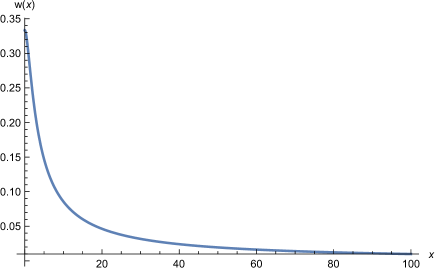
Figure 1: Equation of state $w(x)$ of a particle of mass $m$ at temperature $T$, where $x\equiv mc^{2}/k_{B}T$.

However, the series expansion in powers of $x$ is a little tricky. Expanding the integrand would lead one to expect that the coefficient of the $x^{3}$ term vanishes, and that the $x^{4}$ term diverges,

$$f(x)=\int_{0}^{\infty}\!\!\!\!dt\Bigl{[}t^{2}+2tx+\frac{1}{2}x^{2}+0\cdot\frac{x^{3}}{t}-\frac{x^{4}}{8t^{2}}+\ldots\Bigr{]}e^{-t}\;.$$ (52)

Both expectations are wrong: the $x^{3}$ term has a nonzero coefficient and the next order term is perfectly finite and proportional to $x^{4}\ln(x)$,

$$f(x)=2+2x+\frac{1}{2}x^{2}-\frac{1}{6}x^{3}-\frac{1}{8}x^{4}\ln(x)+O(x^{4})\;.$$ (53)

If such a simple system can develop logarithms in its series expansion, why can this not happen for quantum gravity?

The breakdown of perturbation theory might be tied to the presence of divergences. In a renormalizable theory these divergences are canceled by counterterms, so that the sum of a primitive diagram and the associated counterterm can remain perturbatively small. However, that is precisely what fails in quantum general relativity. Perhaps finiteness comes instead from the gravitational response to divergences? Dvali’s work on classicalization [112, 113] may be relevant.

An old classical calculation by Arnowitt, Deser and Misner provides a thought provoking example [114]. They considered the mass of a point particle with bare mass $M_{0}$ and charge $Q$, regulated as a spherical shell of radius $R$. Although ADM solved the full general relativistic constraints, their result can be understood using a simple model they devised,

$$Mc^{2}=M_{0}c^{2}\!+\!\frac{Q^{2}}{8\pi\epsilon_{0}R}\!-\!\frac{GM^{2}}{2R}\Longrightarrow M(R)=\frac{c^{2}R}{G}\Biggl{[}\sqrt{1\!+\!\frac{2GM_{0}}{Rc^{2}}\!+\!\frac{GQ^{2}}{4\pi\epsilon_{0}R^{2}c^{4}}}-1\Biggr{]}.$$ (54)

Note that the unregulated limit is finite and, interestingly, independent of the bare mass,

$$\lim_{R\rightarrow 0}M(R)=\sqrt{\frac{Q^{2}}{4\pi\epsilon_{0}G}}\;.$$ (55)

This is not at all what one finds using perturbation theory. Expanding the square root in expression (54) reveals an escalating series of ever higher divergences,

$$M(R)=\Bigl{(}M_{0}\!+\!\frac{Q^{2}}{8\pi\epsilon_{0}Rc^{2}}\Bigr{)}\Biggl{\{}1-\frac{1}{4}\Bigl{(}\frac{2GM_{0}}{Rc^{2}}\!+\!\frac{GQ^{2}}{4\pi\epsilon_{0}R^{2}c^{4}}\Bigr{)}$$ (56)

$$\hskip 28.45274pt+\frac{1}{8}\Bigl{(}\frac{2GM_{0}}{Rc^{2}}\!+\!\frac{GQ^{2}}{4\pi\epsilon_{0}R^{2}c^{4}}\Bigr{)}^{2}-\frac{5}{64}\Bigl{(}\frac{2GM_{0}}{Rc^{2}}\!+\!\frac{GQ^{2}}{4\pi\epsilon_{0}R^{2}c^{4}}\Bigr{)}^{3}+\ldots\Biggr{\}}.\qquad$$

Of course perturbation theory is not valid when the expansion parameter becomes infinite. Perhaps the same problem invalidates the use of perturbation theory in quantum general relativity, which would show similar cancellations if only we could devise a better approximation scheme? Several studies have searched for one without success [115, 116, 117, 118], but the amount of effort expended is minuscule compared when compared with the recurrent attempts to rehabilitate the Weyl counterterm.

Cosmology offers an example of the gravitational constraints almost completely canceling scalar perturbations during primordial inflation. Suppose the cosmological scale factor is $a(t)$. Two of its derivatives are the Hubble parameter $H(t)$ and the first slow roll parameter $\epsilon(t)$,

$$H(t)\equiv\frac{\dot{a}}{a}\qquad,\qquad\epsilon(t)\equiv-\frac{\dot{H}}{H^{2}}\;.$$ (57)

Single scalar inflation consists of general relativity plus a minimally coupled inflaton $\varphi$ whose slow roll down its potential $V(\varphi)$ provides the stress-energy of inflation,

$$\mathcal{L}=\frac{c^{4}R\sqrt{-g}}{16\pi G}-\frac{1}{2}\partial_{\mu}\varphi\partial_{\nu}\varphi g^{\mu\nu}\sqrt{-g}-V(\varphi)\sqrt{-g}\;.$$ (58)

The scalar background and its potential are related to the parameters (57),

$$\dot{\varphi}_{0}^{2}=-\frac{c^{4}\dot{H}}{4\pi G}\qquad,\qquad V(\varphi_{0})=\frac{c^{2}(\dot{H}\!+\!3H^{2})}{8\pi G}\;.$$ (59)

It is usual to employ the ADM parameterization for the metric [119],

$$ds^{2}=-N^{2}c^{2}dt^{2}+h_{ij}\Bigl{(}dx^{i}\!-\!N^{i}cdt\Bigr{)}\Bigl{(}dx^{j}\!-\!N^{j}cdt\Bigr{)}\;.$$ (60)

The 3-metric is written in terms of a component $\zeta$ and a traceless part $\chi_{ij}$,

$$h_{ij}(t,\vec{x})\equiv a^{2}(t)\!\times\!e^{2\zeta(t,\vec{x})}\!\times\!\Bigl{[}e^{\chi(t,\vec{x})}\Bigr{]}_{ij}\qquad,\qquad\chi_{ii}(t,\vec{x})=0\;.$$ (61)

Instead of the lapse $N(t,\vec{x})$ and shift $N^{i}(t,\vec{x})$ being gauge choices, the gauge conditions are,

$$\varphi(t,\vec{x})=\varphi_{0}(t)\qquad,\qquad\partial_{j}\chi_{ij}(t,\vec{x})=0\;.$$ (62)

The lapse and shift are instead determined by solving the constraints. The funny thing is, that doing so leads to the almost total cancellation of the scalar perturbation $\zeta(t,\vec{x})$,

$$\mathcal{L}\longrightarrow\frac{c^{4}a^{3}\epsilon}{8\pi G}\Bigl{[}\frac{\dot{\zeta}^{2}}{c^{2}}-\frac{\partial_{k}\zeta\partial_{k}\zeta}{a^{2}}\Bigr{]}+\frac{c^{4}a^{3}}{64\pi G}\Bigl{[}\frac{\dot{\chi}_{ij}\dot{\chi}_{ij}}{c^{2}}-\frac{\partial_{k}\chi_{ij}\partial_{k}\chi_{ij}}{a^{2}}\Bigr{]}+\Bigl{(}{\rm Interactions}\Bigr{)}\;.$$ (63)

Note from (58) that the scalar perturbation had unit strength before imposing the constraints, even after gauge fixing (62). The gravitational constraints have almost completely erased it at the quadratic level (63). Detailed calculations of the constrained interactions [120, 121, 122, 123] show that each additional one or two powers of the scalar perturbation leads to suppression by an additional factor of $\epsilon$. To understand how significant the cancellation is, recall that approximate values for the scalar and tensor power spectra at wave number $k$ can be written in terms of the geometrical parameters (57) evaluated at the horizon crossing time $t_{k}$ such that $ck=H(t_{k})a(t_{k})$,

$$\Delta^{2}_{\mathcal{R}}(k)\simeq\frac{\hbar GH^{2}(t_{k})}{\pi c^{5}\epsilon(t_{k})}\qquad,\qquad\Delta^{2}_{h}(k)\simeq\frac{16\hbar GH^{2}(t_{k})}{\pi c^{5}}\;.$$ (64)

The fact that the scalar power spectrum has been observed, to three significant figures and over a range of about 8 e-foldings [3], while the tensor power spectrum has yet to be resolved [8], means that the first slow roll parameter is very small, $\epsilon\mathrel{\raise 1.29167pt\hbox{$<$\kern-7.5pt\lower 4.30554pt\hbox{$\sim$}}}0.0023$.

5 Conclusions

The gravitational data we currently possess are all either classical [1] or else semi-classical [3]. There is no point to defining a theory of “quantum gravity” which fails to explain these data. This leads to the Quantum Gravitational Correspondence Principle that the classical limit of any proposal for “quantum gravity” must consist of a local, invariant theory of a real-valued metric on a real-valued spacetime. The Correspondence Principle poses an obstacle for modifications of general relativity because we have a complete catalog of such theories and, with the exception of $f(R)$ models, all of them are subject classically to a virulent kinetic energy instability which prevents them even having a finite decay rate. Alternate quantization schemes which claim to avoid this instability fail to obey the Correspondence Principle, and obligate their advocates to explain, in some detail, how they recover the vast body of gravitational phenomena.

These considerations apply to the dimension four Lagrangian (3) which is the focus of many efforts to quantize gravity. In Section 2 I explain how the procedure of regarding negative energy creation operators as positive energy annihilation operators produces the renormalizable, negative norm quantization. This quantization massively violates the Correspondence Principle. One manifestation of this violation is that the square of the time derivative of the geodesic length-squared along a spacelike interval is negative ($[\int\dot{g}_{ij}dx^{i}dx^{j}]^{2}<0$), even over macroscopic separations. This is not some tiny, Planck-suppressed effect; it occurs at order one in the classical limit, and it is totally unacceptable. Note that the negative sign cannot be avoided by careful mathematics, or by further tinkering with the field theory, because it is required for renormalizability.

People who seek to rehabilitate the Weyl counterterm in (3) argue that local fields such as $\dot{g}_{ij}(t,\vec{x})$ are not observable, that the theory can only be defined by the perturbative S-matrix on flat space background, and that the negative norm states are no problem because they not even present in the asymptotic scattering space. Section 3 criticizes this view, pointing out that it is perfectly reasonable to study local fields, and that all current gravitational data — including even the primordial power spectra — are analyzed in precisely this manner. I challenge S-matrix extremists to explain these data using asymptotic scattering theory, without recourse to local fields. It is also worth noting that the quantum gravitational S-matrix fails to exist on flat space background owing to the infrared problem, and that even inclusive rates and cross sections are unlikely to exist or be observable in cosmology. Note that the problem with observability is not some subtle issue which might be circumvented with careful mathematics; it is rather that causality and spacetime expansion preclude performing the required measurements.

The really crushing argument against S-matrix chauvinism comes in Section 3.3 where I present a nonlinear sigma model (31) on de Sitter background which is reducible to a free theory by a local, invertible field redefinition (32-33). This means that its S-matrix is unity and, if we adhere to S-matrix chauvinism, nothing interesting happens in the theory. But the scalar background still shows a fascinating evolution (35), leading to corresponding changes in the masses (36) of single particles, all despite the absence of scattering.

It seems to me that the attention devoted to high energy scattering theory and to black hole evaporation have led us away from the testable and exciting things quantum gravity can do for us in the context of low energy effective field theory [10, 11, 12, 13, 14, 15]. Section 4 reviews my own favorites. I also discuss the possibility that we should take seriously the difficulty of modifying general relativity and focus instead on the inappropriate application of perturbation theory such as expression (56) when the actual series expansion includes fractional powers or logarithms of $G$.

Finally, I should comment that either possibility for the viability of the dimension four Lagrangian (3) is problematic for the program of Asymptotic Safety [54, 55, 56]. Either the Weyl counterterm is permitted or it is not. If it is allowed then (3) is perturbatively renormalizable, and we have the ultraviolet completion of general relativity, without the need for any higher counterterms. On the other hand, if the Weyl counterterm is not permitted then most of the higher counterterms are also forbidden, and those from $f(R)$ extensions will not suffice to absorb all divergences. Either way, motivation is lacking to search for fixed points of the infinite collection of higher counterterms. If we instead treat the higher counterterms perturbatively, in the sense of low energy effective field theory [10, 11, 12, 13, 14, 15], then their unknown coefficients pose no problem to predictability, in any existing or projected data sets, as long as their coefficients are of order one in Planck units.

That last caveat, about the unknown coefficients being of order one in Planck units, is significant because violations have been proposed for $f(R)$ models, which are the sole allowed extensions of general relativity. In particular, permitting the $R^{2}$ coefficient $\alpha$ to be as large as $10^{10}$ provides a model of inflation [17] which agrees well with existing data [19]. $f(R)$ models can also explain late time acceleration within observational limits [124]. It would be a huge triumph for Asymptotic Safety to justify these models.

Acknowledgements

I am grateful for civil discussion and correspondence on this subject with J. F. Donoghue, B. Holdom and P. D. Mannheim. This work was supported by NSF grant PHY-2207514 and by the Institute for Fundamental Theory at the University of Florida.

References

- [1] C. M. Will, Living Rev. Rel. 17, 4 (2014) doi:10.12942/lrr-2014-4 [arXiv:1403.7377 [gr-qc]].
- [2] V. F. Mukhanov and G. V. Chibisov, JETP Lett. 33, 532-535 (1981)
- [3] N. Aghanim et al. [Planck], Astron. Astrophys. 641, A1 (2020) doi:10.1051/0004-6361/201833880 [arXiv:1807.06205 [astro-ph.CO]].
- [4] A. Loeb and M. Zaldarriaga, Phys. Rev. Lett. 92, 211301 (2004) doi:10.1103/PhysRevLett.92.211301 [arXiv:astro-ph/0312134 [astro-ph]].
- [5] S. Furlanetto, S. P. Oh and F. Briggs, Phys. Rept. 433, 181-301 (2006) doi:10.1016/j.physrep.2006.08.002 [arXiv:astro-ph/0608032 [astro-ph]].
- [6] K. W. Masui and U. L. Pen, Phys. Rev. Lett. 105, 161302 (2010) doi:10.1103/PhysRevLett.105.161302 [arXiv:1006.4181 [astro-ph.CO]].
- [7] A. A. Starobinsky, JETP Lett. 30, 682-685 (1979)
- [8] P. A. R. Ade et al. [BICEP and Keck], Phys. Rev. Lett. 127, no.15, 151301 (2021) doi:10.1103/PhysRevLett.127.151301 [arXiv:2110.00483 [astro-ph.CO]].
- [9] L. Tan, N. C. Tsamis and R. P. Woodard, Phil. Trans. Roy. Soc. Lond. A 380, 0187 (2021) doi:10.1098/rsta.2021.0187 [arXiv:2107.13905 [gr-qc]].
- [10] J. F. Donoghue, Phys. Rev. D 50, 3874-3888 (1994) doi:10.1103/PhysRevD.50.3874 [arXiv:gr-qc/9405057 [gr-qc]].
- [11] J. F. Donoghue, [arXiv:gr-qc/9512024 [gr-qc]].
- [12] C. P. Burgess, Living Rev. Rel. 7, 5-56 (2004) doi:10.12942/lrr-2004-5 [arXiv:gr-qc/0311082 [gr-qc]].
- [13] J. F. Donoghue, AIP Conf. Proc. 1483, no.1, 73-94 (2012) doi:10.1063/1.4756964 [arXiv:1209.3511 [gr-qc]].
- [14] J. Donoghue, Scholarpedia 12, no.4, 32997 (2017) doi:10.4249/scholarpedia.32997
- [15] J. F. Donoghue, [arXiv:2211.09902 [hep-th]].
- [16] K. S. Stelle, Phys. Rev. D 16, 953-969 (1977) doi:10.1103/PhysRevD.16.953
- [17] A. A. Starobinsky, Phys. Lett. B 91, 99-102 (1980) doi:10.1016/0370-2693(80)90670-X
- [18] N. Aghanim et al. [Planck], Astron. Astrophys. 641, A6 (2020) [erratum: Astron. Astrophys. 652, C4 (2021)] doi:10.1051/0004-6361/201833910 [arXiv:1807.06209 [astro-ph.CO]].
- [19] Y. Akrami et al. [Planck], Astron. Astrophys. 641, A10 (2020) doi:10.1051/0004-6361/201833887 [arXiv:1807.06211 [astro-ph.CO]].
- [20] R. P. Woodard, Rept. Prog. Phys. 72, 126002 (2009) doi:10.1088/0034-4885/72/12/126002 [arXiv:0907.4238 [gr-qc]].
- [21] B. S. DeWitt, Phys. Rev. 160, 1113-1148 (1967) doi:10.1103/PhysRev.160.1113
- [22] B. S. DeWitt, Phys. Rev. 162, 1195-1239 (1967) doi:10.1103/PhysRev.162.1195
- [23] B. S. DeWitt, Phys. Rev. 162, 1239-1256 (1967) doi:10.1103/PhysRev.162.1239
- [24] G. ’t Hooft and M. J. G. Veltman, Ann. Inst. H. Poincare Phys. Theor. A 20, 69-94 (1974)
- [25] S. Deser and P. van Nieuwenhuizen, Phys. Rev. Lett. 32, 245-247 (1974) doi:10.1103/PhysRevLett.32.245
- [26] S. Deser and P. van Nieuwenhuizen, Phys. Rev. D 10, 401 (1974) doi:10.1103/PhysRevD.10.401
- [27] S. Deser and P. van Nieuwenhuizen, Phys. Rev. D 10, 411 (1974) doi:10.1103/PhysRevD.10.411
- [28] S. Deser, H. S. Tsao and P. van Nieuwenhuizen, Phys. Lett. B 50, 491-493 (1974) doi:10.1016/0370-2693(74)90268-8
- [29] S. Deser, H. S. Tsao and P. van Nieuwenhuizen, Phys. Rev. D 10, 3337 (1974) doi:10.1103/PhysRevD.10.3337
- [30] M. H. Goroff and A. Sagnotti, Phys. Lett. B 160, 81-86 (1985) doi:10.1016/0370-2693(85)91470-4
- [31] M. H. Goroff and A. Sagnotti, Nucl. Phys. B 266, 709-736 (1986) doi:10.1016/0550-3213(86)90193-8
- [32] A. E. M. van de Ven, Nucl. Phys. B 378, 309-366 (1992) doi:10.1016/0550-3213(92)90011-Y
- [33] E. Tomboulis, Phys. Lett. B 70, 361-364 (1977) doi:10.1016/0370-2693(77)90678-5
- [34] A. Salam and J. A. Strathdee, Phys. Rev. D 18, 4480 (1978) doi:10.1103/PhysRevD.18.4480
- [35] I. Antoniadis and N. C. Tsamis, Phys. Lett. B 144, 55-60 (1984) doi:10.1016/0370-2693(84)90175-8
- [36] I. Antoniadis and E. T. Tomboulis, Phys. Rev. D 33, 2756 (1986) doi:10.1103/PhysRevD.33.2756
- [37] D. A. Johnston, Nucl. Phys. B 297, 721-732 (1988) doi:10.1016/0550-3213(88)90555-X
- [38] S. W. Hawking and T. Hertog, Phys. Rev. D 65, 103515 (2002) doi:10.1103/PhysRevD.65.103515 [arXiv:hep-th/0107088 [hep-th]].
- [39] F. d. Salles and I. L. Shapiro, Phys. Rev. D 89, no.8, 084054 (2014) [erratum: Phys. Rev. D 90, no.12, 129903 (2014)] doi:10.1103/PhysRevD.89.084054 [arXiv:1401.4583 [hep-th]].
- [40] F. de O.Salles and I. L. Shapiro, Universe 4, no.9, 91 (2018) doi:10.3390/universe4090091 [arXiv:1808.09015 [gr-qc]].
- [41] J. F. Donoghue and G. Menezes, Phys. Rev. D 100, no.10, 105006 (2019) doi:10.1103/PhysRevD.100.105006 [arXiv:1908.02416 [hep-th]].
- [42] J. F. Donoghue and G. Menezes, Phys. Rev. Lett. 123, no.17, 171601 (2019) doi:10.1103/PhysRevLett.123.171601 [arXiv:1908.04170 [hep-th]].
- [43] P. D. Mannheim, Int. J. Mod. Phys. D 29, no.14, 2043009 (2020) doi:10.1142/S0218271820430099 [arXiv:2004.00376 [hep-th]].
- [44] J. F. Donoghue and G. Menezes, Phys. Rev. D 104, no.4, 045010 (2021) doi:10.1103/PhysRevD.104.045010 [arXiv:2105.00898 [hep-th]].
- [45] B. Holdom, Phys. Rev. D 105, no.4, 046008 (2022) doi:10.1103/PhysRevD.105.046008 [arXiv:2107.01727 [hep-th]].
- [46] P. D. Mannheim, Nuovo Cim. C 45, no.2, 27 (2022) doi:10.1393/ncc/i2022-22027-6 [arXiv:2109.12743 [hep-th]].
- [47] P. D. Mannheim, [arXiv:2303.10827 [hep-th]].
- [48] T. D. Lee and G. C. Wick, Nucl. Phys. B 9, 209-243 (1969) doi:10.1016/0550-3213(69)90098-4
- [49] T. D. Lee and G. C. Wick, Phys. Rev. D 2, 1033-1048 (1970) doi:10.1103/PhysRevD.2.1033
- [50] B. Grinstein, D. O’Connell and M. B. Wise, Phys. Rev. D 77, 025012 (2008) doi:10.1103/PhysRevD.77.025012 [arXiv:0704.1845 [hep-ph]].
- [51] J. F. Donoghue and G. Menezes, Phys. Rev. D 99, no.6, 065017 (2019) doi:10.1103/PhysRevD.99.065017 [arXiv:1812.03603 [hep-th]].
- [52] C. M. Bender and P. D. Mannheim, Phys. Rev. Lett. 100, 110402 (2008) doi:10.1103/PhysRevLett.100.110402 [arXiv:0706.0207 [hep-th]].
- [53] C. M. Bender and P. D. Mannheim, J. Phys. A 41, 304018 (2008) doi:10.1088/1751-8113/41/30/304018 [arXiv:0807.2607 [hep-th]].
- [54] M. Niedermaier and M. Reuter, Living Rev. Rel. 9, 5-173 (2006) doi:10.12942/lrr-2006-5
- [55] D. Benedetti, P. F. Machado and F. Saueressig, Mod. Phys. Lett. A 24, 2233-2241 (2009) doi:10.1142/S0217732309031521 [arXiv:0901.2984 [hep-th]].
- [56] K. G. Falls, D. F. Litim and J. Schröder, Phys. Rev. D 99, no.12, 126015 (2019) doi:10.1103/PhysRevD.99.126015 [arXiv:1810.08550 [gr-qc]].
- [57] M. Ostrogradsky, Mem. Acad. St. Petersbourg 6, no.4, 385-517 (1850)
- [58] R. P. Woodard, Scholarpedia 10, no.8, 32243 (2015) doi:10.4249/scholarpedia.32243 [arXiv:1506.02210 [hep-th]].
- [59] R. P. Woodard, Lect. Notes Phys. 720, 403-433 (2007) doi:10.1007/978-3-540-71013-4_14 [arXiv:astro-ph/0601672 [astro-ph]].
- [60] J. M. Cline, S. Jeon and G. D. Moore, Phys. Rev. D 70, 043543 (2004) doi:10.1103/PhysRevD.70.043543 [arXiv:hep-ph/0311312 [hep-ph]].
- [61] C. Deffayet, A. Held, S. Mukohyama and A. Vikman, [arXiv:2305.09631 [gr-qc]].
- [62] D. G. Boulware, G. T. Horowitz and A. Strominger, Phys. Rev. Lett. 50, 1726 (1983) doi:10.1103/PhysRevLett.50.1726
- [63] A. Mostafazadeh, [arXiv:quant-ph/0310164 [quant-ph]].
- [64] A. Mostafazadeh and A. Batal, J. Phys. A 37, 11645-11680 (2004) doi:10.1088/0305-4470/37/48/009 [arXiv:quant-ph/0408132 [quant-ph]].
- [65] A. Mostafazadeh, Phys. Scripta 82, 038110 (2010) doi:10.1088/0031-8949/82/03/038110 [arXiv:1008.4680 [quant-ph]].
- [66] J. D. Jackson, Wiley, 1998, ISBN 978-0-471-30932-1
- [67] K. E. Leonard and R. P. Woodard, Phys. Rev. D 85, 104048 (2012) doi:10.1103/PhysRevD.85.104048 [arXiv:1202.5800 [gr-qc]].
- [68] J. S. Schwinger, J. Math. Phys. 2, 407-432 (1961) doi:10.1063/1.1703727
- [69] K. T. Mahanthappa, Phys. Rev. 126, 329-340 (1962) doi:10.1103/PhysRev.126.329
- [70] P. M. Bakshi and K. T. Mahanthappa, J. Math. Phys. 4, 1-11 (1963) doi:10.1063/1.1703883
- [71] P. M. Bakshi and K. T. Mahanthappa, J. Math. Phys. 4, 12-16 (1963) doi:10.1063/1.1703879
- [72] L. V. Keldysh, Zh. Eksp. Teor. Fiz. 47, 1515-1527 (1964)
- [73] K. c. Chou, Z. b. Su, B. l. Hao and L. Yu, Phys. Rept. 118, 1-131 (1985) doi:10.1016/0370-1573(85)90136-X
- [74] R. D. Jordan, Phys. Rev. D 33, 444-454 (1986) doi:10.1103/PhysRevD.33.444
- [75] E. Calzetta and B. L. Hu, Phys. Rev. D 35, 495 (1987) doi:10.1103/PhysRevD.35.495
- [76] L. H. Ford and R. P. Woodard, Class. Quant. Grav. 22, 1637-1647 (2005) doi:10.1088/0264-9381/22/9/011 [arXiv:gr-qc/0411003 [gr-qc]].
- [77] S. P. Miao, T. Prokopec and R. P. Woodard, Phys. Rev. D 96, no.10, 104029 (2017) doi:10.1103/PhysRevD.96.104029 [arXiv:1708.06239 [gr-qc]].
- [78] S. Katuwal and R. P. Woodard, JHEP 21, 029 (2020) doi:10.1007/JHEP10(2021)029 [arXiv:2107.13341 [gr-qc]].
- [79] S. Weinberg, Phys. Rev. 140, B516-B524 (1965) doi:10.1103/PhysRev.140.B516
- [80] G. Veneziano, Nucl. Phys. B 44, 142-148 (1972) doi:10.1016/0550-3213(72)90275-1
- [81] D. Marolf, I. A. Morrison and M. Srednicki, Class. Quant. Grav. 30, 155023 (2013) doi:10.1088/0264-9381/30/15/155023 [arXiv:1209.6039 [hep-th]].
- [82] S. P. Miao, N. C. Tsamis and R. P. Woodard, JHEP 03, 069 (2022) doi:10.1007/JHEP03(2022)069 [arXiv:2110.08715 [gr-qc]].
- [83] H. J. Borchers, Il Nuovo Cimento 15, 784-794 (1960) doi.org/10.1007/BF02732693.
- [84] R. P. Woodard and B. Yesilyurt, [arXiv:2302.11528 [gr-qc]].
- [85] D. Glavan, S. P. Miao, T. Prokopec and R. P. Woodard, Class. Quant. Grav. 31, 175002 (2014) doi:10.1088/0264-9381/31/17/175002 [arXiv:1308.3453 [gr-qc]].
- [86] C. L. Wang and R. P. Woodard, Phys. Rev. D 91, no.12, 124054 (2015) doi:10.1103/PhysRevD.91.124054 [arXiv:1408.1448 [gr-qc]].
- [87] S. P. Miao and R. P. Woodard, Phys. Rev. D 74, 024021 (2006) doi:10.1103/PhysRevD.74.024021 [arXiv:gr-qc/0603135 [gr-qc]].
- [88] D. Glavan, S. P. Miao, T. Prokopec and R. P. Woodard, JHEP 03, 088 (2022) doi:10.1007/JHEP03(2022)088 [arXiv:2112.00959 [gr-qc]].
- [89] L. Tan, N. C. Tsamis and R. P. Woodard, Universe 8, no.7, 376 (2022) doi:10.3390/universe8070376 [arXiv:2206.11467 [gr-qc]].
- [90] V. K. Onemli and R. P. Woodard, Class. Quant. Grav. 19, 4607 (2002) doi:10.1088/0264-9381/19/17/311 [arXiv:gr-qc/0204065 [gr-qc]].
- [91] V. K. Onemli and R. P. Woodard, Phys. Rev. D 70, 107301 (2004) doi:10.1103/PhysRevD.70.107301 [arXiv:gr-qc/0406098 [gr-qc]].
- [92] A. A. Starobinsky, Lect. Notes Phys. 246, 107-126 (1986) doi:10.1007/3-540-16452-9_6
- [93] A. A. Starobinsky and J. Yokoyama, Phys. Rev. D 50, 6357-6368 (1994) doi:10.1103/PhysRevD.50.6357 [arXiv:astro-ph/9407016 [astro-ph]].
- [94] C. Litos, R. P. Woodard and B. Yesilyurt, University of Florida preprint UFIFT-QG-23-07, in preparation.
- [95] W. Pauli, Helv. Phys. Acta Suppl. 4, 58-71 (1956)
- [96] S. Deser, Rev. Mod. Phys. 29, 417 (1957) doi:10.1103/RevModPhys.29.417
- [97] L. H. Ford, Int. J. Theor. Phys. 44, 1753-1768 (2005) doi:10.1007/s10773-005-8893-z [arXiv:gr-qc/0501081 [gr-qc]].
- [98] A. Marunovic and T. Prokopec, Phys. Rev. D 83, 104039 (2011) doi:10.1103/PhysRevD.83.104039 [arXiv:1101.5059 [gr-qc]].
- [99] K. E. Leonard and R. P. Woodard, Class. Quant. Grav. 31, 015010 (2014) doi:10.1088/0264-9381/31/1/015010 [arXiv:1304.7265 [gr-qc]].
- [100] A. F. Radkowski, Ann. Phys. 56, 319-354 (1970) doi:10.1016/0003-4916(70)90021-7
- [101] E. Kasdagli, M. Ulloa and R. P. Woodard, Phys. Rev. D 107, no.10, 105023 (2023) doi:10.1103/PhysRevD.107.105023 [arXiv:2302.04808 [gr-qc]].
- [102] R. P. Woodard and B. Yesilyurt, [arXiv:2305.17641 [gr-qc]].
- [103] P. Horava, JHEP 03, 020 (2009) doi:10.1088/1126-6708/2009/03/020 [arXiv:0812.4287 [hep-th]].
- [104] P. Horava, Phys. Rev. D 79, 084008 (2009) doi:10.1103/PhysRevD.79.084008 [arXiv:0901.3775 [hep-th]].
- [105] S. Mukohyama, Class. Quant. Grav. 27, 223101 (2010) doi:10.1088/0264-9381/27/22/223101 [arXiv:1007.5199 [hep-th]].
- [106] A. O. Barvinsky, D. Blas, M. Herrero-Valea, S. M. Sibiryakov and C. F. Steinwachs, Phys. Rev. D 93, no.6, 064022 (2016) doi:10.1103/PhysRevD.93.064022 [arXiv:1512.02250 [hep-th]].
- [107] S. Carlip, Stud. Hist. Phil. Sci. B 46, 200-208 (2014) doi:10.1016/j.shpsb.2012.11.002 [arXiv:1207.2504 [gr-qc]].
- [108] E. P. Verlinde, SciPost Phys. 2, no.3, 016 (2017) doi:10.21468/SciPostPhys.2.3.016 [arXiv:1611.02269 [hep-th]].
- [109] S. Hossenfelder, Phys. Rev. D 95, no.12, 124018 (2017) doi:10.1103/PhysRevD.95.124018 [arXiv:1703.01415 [gr-qc]].
- [110] J. Ambjorn, A. Goerlich, J. Jurkiewicz and R. Loll, Phys. Rept. 519, 127-210 (2012) doi:10.1016/j.physrep.2012.03.007 [arXiv:1203.3591 [hep-th]].
- [111] J. Ambjorn, J. Gizbert-Studnicki, A. Görlich, J. Jurkiewicz and R. Loll, Front. in Phys. 8, 247 (2020) doi:10.3389/fphy.2020.00247 [arXiv:2002.01693 [hep-th]].
- [112] G. Dvali, G. F. Giudice, C. Gomez and A. Kehagias, JHEP 08, 108 (2011) doi:10.1007/JHEP08(2011)108 [arXiv:1010.1415 [hep-ph]].
- [113] G. Dvali, C. Gomez, R. S. Isermann, D. Lüst and S. Stieberger, Nucl. Phys. B 893, 187-235 (2015) doi:10.1016/j.nuclphysb.2015.02.004 [arXiv:1409.7405 [hep-th]].
- [114] R. Arnowitt, S. Deser and C. W. Misner, Phys. Rev. Lett. 4, 375-377 (1960) doi:10.1103/PhysRevLett.4.375
- [115] R. P. Woodard, [arXiv:gr-qc/9803096 [gr-qc]].
- [116] R. Casadio, J. Phys. Conf. Ser. 174, 012058 (2009) doi:10.1088/1742-6596/174/1/012058 [arXiv:0902.2939 [gr-qc]].
- [117] R. Casadio, R. Garattini and F. Scardigli, Phys. Lett. B 679, 156-159 (2009) doi:10.1016/j.physletb.2009.06.076 [arXiv:0904.3406 [gr-qc]].
- [118] P. J. Mora, N. C. Tsamis and R. P. Woodard, Class. Quant. Grav. 29, 025001 (2012) doi:10.1088/0264-9381/29/2/025001 [arXiv:1108.4367 [gr-qc]].
- [119] R. L. Arnowitt, S. Deser and C. W. Misner, Phys. Rev. 116, 1322-1330 (1959) doi:10.1103/PhysRev.116.1322
- [120] J. M. Maldacena, JHEP 05, 013 (2003) doi:10.1088/1126-6708/2003/05/013 [arXiv:astro-ph/0210603 [astro-ph]].
- [121] D. Seery, J. E. Lidsey and M. S. Sloth, JCAP 01, 027 (2007) doi:10.1088/1475-7516/2007/01/027 [arXiv:astro-ph/0610210 [astro-ph]].
- [122] P. R. Jarnhus and M. S. Sloth, JCAP 02, 013 (2008) doi:10.1088/1475-7516/2008/02/013 [arXiv:0709.2708 [hep-th]].
- [123] W. Xue, X. Gao and R. Brandenberger, JCAP 06, 035 (2012) doi:10.1088/1475-7516/2012/06/035 [arXiv:1201.0768 [hep-th]].
- [124] A. A. Starobinsky, JETP Lett. 86, 157-163 (2007) doi:10.1134/S0021364007150027 [arXiv:0706.2041 [astro-ph]].