Training generative models from privatized data

Abstract

Local differential privacy (LDP) is a powerful method for privacy-preserving data collection. In this paper, we develop a framework for training Generative Adversarial Networks (GAN) on differentially privatized data. We show that entropic regularization of the Wasserstein distance – a popular regularization method in the literature that has been often leveraged for its computational benefits – can be used to denoise the data distribution when data is privatized by common additive noise mechanisms, such as Laplace and Gaussian. This combination uniquely enables the mitigation of both the regularization bias and the effects of privatization noise, thereby enhancing the overall efficacy of the model. We analyse the proposed method, provide sample complexity results and experimental evidence to support its efficacy.

1 Introduction

Local differential privacy [Dwork et al., 2006a, Kasiviswanathan et al., 2011] has emerged as a powerful method to provide privacy guarantees on individuals’ personal data and has been recently deployed by major technology organizations for privacy-preserving data collection from peripheral devices. In this framework, the user data is locally randomized (e.g. by the addition of noise) before it is transferred to the data curator, so the privacy guarantee does not rely on a trusted centralized server. Mathematically provable guarantees on the randomization mechanism ensure that any adversary that gets access to the privatized data will be unable to learn too much about the user’s personal information. This directly alleviates many of the systematic privacy and security challenges associated with traditional data collection including those around transparency, data misuse, control, compliance with regulatory strictures, breaches, processing, and release. Learning from privatized data, however, requires rethinking machine learning methods to extract accurate and useful population-level models from the noisy individual data.

In this paper, we consider the problem of training generative models from locally privatized user data. In recent years, deep learning based generative models, known as Generative Adverserial Networks (GANs), have become a popular framework for learning data distributions and sampling as they have achieved impressive results in various domains [De et al., 2016, Isola et al., 2017, Reed et al., 2016, Ledig et al., 2017]. As opposed to traditional methods of fitting a parametric distribution, GANs aim to learn a mapping (usually modeled as a neural network) from a simple known distribution to the unknown data distribution or its empirical approximation. The mapping is set to a minimizer of a chosen distance measure between the generated and target distributions. A popular metric used in practice is the $p$-Wasserstein distance (see Section 2 for a formal definition), in which case the GAN optimization problem can be written in the following form,

$$\min_{G\in\mathcal{G}}W_{p}^{p}\left({P}_{G(Z)},{P}_{X}\right).$$ (1)

Here $G(\cdot)$ is called the generator, which comes from a set of functions ${\mathcal{G}\subseteq\{G:\mathcal{Z}\to\mathcal{X}\}}$ and maps a latent random variable $Z\in\mathcal{Z}$ with some known distribution to a random variable $G(Z)\in\mathcal{X}$, with distribution ${P}_{G(Z)}$ that is close to some target probability measure $P_{X}$ in $p$-Wasserstein distance. The target probability measure $P_{X}$ is the population distribution from which samples $\{X_{i}\}_{i=1}^{n}\sim P_{X}^{\otimes n}$ are drawn and the optimization problem is solved by replacing $P_{X}$ in (1) with the empirical distribution ${Q}_{X}^{n}$ of the samples. For example, $X_{i}$ can represent images taken by users in which case $G$ represents a generative model for such images.

How can we use the GAN framework above to learn a generative model for $P_{X}$ when we have only access to samples privatized by an LDP mechanism? Assume each $X_{i}$ represents a sample locally generated at user $i$, and is transferred to the learner after processing it with an LDP mechanism $M:\mathcal{X}\rightarrow\mathcal{Y}$, i.e., the learner only observes the privatized samples $\{Y_{i}=M(X_{i})\}_{i=1}^{n}$. Can we learn a generative model for the true distribution $P_{X}$ from the privatized samples ${Y_{i}}_{i=1}^{n}$? Simply replacing the target distribution $P_{X}$ in (1) with the empirical distribution ${Q}_{Y}^{n}$ of the observed samples,

$$\min_{G\in\mathcal{G}}W_{p}^{p}\left({P}_{G(Z)},{Q}_{Y}^{n}\right),$$ (2)

will result in a generative model for $P_{Y}=M\#P_{X}$, the push-forward distribution of $P_{X}$ through the privatization mechanism $M$, rather than the original distribution $P_{X}$. In other words, we will learn to generate the privatized data (e.g., noisy images) instead of learning to generate the original (raw) data.

In this paper, we show that a simple but non-intuitive modification of the objective in (2) – the addition of an entropic regularization term – allows one to provably learn the original distribution of the samples under de-facto privatization mechanisms such as the local Laplace or Gaussian mechanism. We first show that in the population case when ${Q}_{Y}^{n}$ is replaced by $P_{Y}=M\#P_{X}$, the optimal solution $G^{*}$ of the entropic $p$-Wasserstein GAN is such that ${P}_{G^{*}(Z)}=P_{X}$ (assuming $\mathcal{G}$ is rich enough to generate $P_{X}$). Here, $p$ is chosen to match the privatization mechanism used, e.g. $p=1$ for the Laplace mechanism and $p=2$ for the Gaussian mechanism. This result shows that the entropic regularization acts as a denoiser for the Gaussian mechanism under the $W_{2}$ distance, and the Laplace mechanism under the $W_{1}$ distance. See Section 3 for the statement of our result for general $p\geq 1$. We also provide sample complexity results which suggest that the solution of the empirical problem (when $P_{Y}$ is replaced by ${Q}_{Y}^{n}$) converges to the population solution at the parametric convergence rate $O(1/\sqrt{n})$.

Entropic regularization for Wasserstein GANs has been of significant interest in the prior literature, albeit for different reasons. Historically, it has been leveraged primarily for its computational benefits, enabling a more efficient approximation of the optimal transport problem. Its capacity to facilitate rapid convergence and circumvent the curse of dimensionality has made it a popular choice in a variety of applications, from machine learning to optimal transport and beyond. Without regularization, it is known that even when the generators are restricted to be linear, the solution of 1 converges to the optimal solution as $\Omega(n^{-2/d})$ [Feizi et al., 2020], where $d$ is the dimension of the target distribution ($P_{X}$) in contrast to the parametric convergence rate $O(1/\sqrt{n})$. From the perspective of this literature, our result provides a new application for entropy regularization. We demonstrate that, when applied thoughtfully, entropy regularization can facilitate the learning of the original data distribution even when the data has been subjected to a noise injection for privacy preservation. This expands our understanding of the potential applications and benefits of entropy regularization, demonstrating its versatility and capacity to enhance outcomes in a privacy-preserving context.

We note that a significant advantage of our framework is its compatibility with the existing entropic transport libraries Flamary et al. [2021], Feydy et al. [2019]. This can enable researchers to utilize these libraries as a black-box component, streamlining the overall process. This convenience is largely due to use of local DP, where privatization occurs exclusively at the data level, while DP-SGD [Song et al., 2013] based methods [Chen et al., 2020a, Cao et al., 2021, Xie et al., 2018, Zhang et al., 2018] as well as Private Aggregation based methods [Papernot et al., 2018, 2016] privatize the training process, which often necessitates modifications or adaptations at the training stage. By localizing the privatization process to the data level, we ensure that the training of privatized samples is effectively indistinguishable from training a non-privatized version of a GAN (with entropic regularization). Interestingly, when entropic regularization is used with raw (unprivatized) samples it is known to often require de-biasing and lead to blurry results [Feydy et al., 2019, Seguy et al., 2017]. In contrast, our experimental results reveal a somewhat surprising outcome. When we introduce noise to the data, not only does it serve to privatize the data, but it also results in superior output performance. From the perspective of our result in Theorem • ‣ 1, this can be understood as follows. Entropic regularization inherently denoises the target distribution as if it has already been corrupted by noise. When the target distribution is not noisy, this leads to a corruption of the generated distribution and therefore blurry results.

The contributions of our paper can be summarized as follows:

• LDP Framework for Wasserstein GANs: We propose a novel modification to the widely adopted Wasserstein GAN framework that enables it to learn effectively from LDP samples with only one communication round between the data holders and the server. This adaptation, which is both simple and non-intuitive, provides a solution for privacy-preserving learning that does not require any training method modifications.

• Sample Complexity Bounds: An essential element of our work involves providing sample complexity bounds. These bounds offer theoretical insights into the performance and scalability of our proposed method, providing a clear understanding of the trade-off between privacy, accuracy, and the volume of data.

• Empirical Validation: We supplement our theoretical contributions with a comprehensive set of experiments designed to validate our claims. These experiments demonstrate the efficacy of our approach in practical scenarios and provide empirical evidence of the superior performance of our method.

1.1 Related Work

Estimation, inference and learning problems under local differential privacy constraints have been of significant interest in the recent literature with emphasis on two canonical tasks: discrete distribution and mean estimation Bassily et al. [2017], Bun et al. [2019], Chen et al. [2021, 2020b], Suresh et al. [2017], Bhowmick et al. [2018], Han et al. [2018]. The works have characterised the optimal (order-optimal) LDP mechanisms for both problems as well as sample complexity bounds that reveal the impact of the local privacy constraint on estimation accuracy. However, insights from these solutions do not extend to learning high-dimensional distributions under LDP constraints. In discrete distribution estimation, the alphabet is assumed to be discrete and finite, and private mean estimation leverages the fact that averaging the privatized samples provides an unbaised estimate of the mean. None of these assumptions are applicable in our case. The understanding of learning problems under LDP constraints is relatively limited, and even less so in the non-interactive setting when the data is accessed only once, which can be exponentially harder to train as shown in Kasiviswanathan et al. [2011], Bhowmick et al. [2018].

The exploration of differentially private learning in generative models has primarily been focused on introducing privacy during the training phase, e.g. by adding noise to the gradients during training.Chen et al. [2020a], Cao et al. [2021], Xie et al. [2018], Zhang et al. [2018]. While GANs have demonstrated capabilities in synthesizing intricate data, such as high-definition images in a non-private setting Isola et al. [2017], their implementation within a private context presents considerable challenges. This is partly due to the inherent instability during GANs’ training process Arjovsky and Bottou [2017], Mescheder et al. [2018], which can be amplified when noise is introduced into the GAN’s gradients during training - a prevalent practice in implementing differential privacy. Even-though, such instabilities can be mitigated by meticulous hyperparameter tuning, this contradicts the essence of privacy that aims to minimize repeated data access Chaudhuri and Vinterbo [2013]. Privatizing the gradients locally, e.g. in a federated learning setting, and transmitting them between the data holder and the server can lead to a large communication overhead since the model and its gradients are transmitted every iteration of the learning algorithm Mansbridge et al. [2020]. In contrast, in our framework privatization is achieved at the data level, and the training of the GAN is effectively indistinguishable from the non-private case.

2 Background and Problem Formulation

To formally state the problem we first introduce the necessary concepts of privacy.

2.1 Local Differential Privacy

Local Differential Privacy. Warner [1965], Evfimievski et al. [2003], Dwork et al. [2006a], Kasiviswanathan et al. [2011] Local randomized algorithm $\mathcal{A}:\mathcal{X}\to\mathcal{Z}$ acting on the data domain $\mathcal{X}$, satisfies $\epsilon$-local differential privacy for $\epsilon\geq 0,$ if for any $S\subseteq\mathcal{Z}$ and for any pair of inputs $x,x^{\prime}\in\mathcal{X}$ it holds that

$$P(\mathcal{A}(x)\in S)\leq e^{\epsilon}P(\mathcal{A}(x^{\prime})\in S)$$ (3)

LDP ensures that the input to $\mathcal{A}$ cannot be determined from its output with high confidence (determined by $\epsilon$). One of the most common ways of achieving local differential privacy is via the Laplace mechanism.

Laplace Mechanism Dwork et al. [2006a]. For any $\epsilon>0$ and any function $f:\mathcal{X}\to\mathbb{R}^{k}$ such that $\|f(x)-f(x^{\prime})\|_{1}\leq\Delta$ for any $x,x^{\prime}\in\mathcal{X},$ the randomized mechanism $\mathcal{A}(x)=f(x)+(s_{1},\ldots,s_{k})$ with $s_{i}\sim\text{Laplace}(0,\Delta/\epsilon)$ independent of $s_{j},j\neq i$ is $\epsilon$-DP and is called the Laplace Mechanism. We will call $\epsilon/\Delta$ the noise scale of the mechanism.

Approximate Local Differential Privacy. Local randomized algorithm $\mathcal{A}:\mathcal{X}\to\mathcal{Z}$ acting on the data domain $\mathcal{X}$, satisfies $(\epsilon,\delta)$- (approximate) local differential privacy for $\epsilon\geq 0,\delta\in(0,1)$ if for any $S\subseteq\mathcal{Z}$ and for any pair of inputs $x,x^{\prime}\in\mathcal{X}$ it holds that

$$P(\mathcal{A}(x)\in S)\leq e^{\epsilon}P(\mathcal{A}(x^{\prime})\in S)+\delta$$ (4)

$(\epsilon,\delta)$-LDP is very similar to pure LDP, but it allows privacy to be violated with (small) probability $\delta.$ One of the most versatile mechanisms to achieve $(\epsilon,\delta)$-DP is the Gaussian Mechanism.

Gaussian Mechanism Dwork et al. [2006b, 2014], Zhao et al. [2019] For any $\epsilon>0,$ $\delta\in(0,0.5),$ and any function $f:\mathcal{X}\to\mathbb{R}^{k}$ such that $\|f(x)-f(x^{\prime})\|_{2}\leq\Delta$ for any $x,x^{\prime}\in\mathcal{X},$ the randomized mechanism $\mathcal{A}(x)=f(x)+(s_{1},\ldots,s_{k})$ with $s_{i}\sim\mathcal{N}(0,\sigma^{2})$ independent of $s_{j},j\neq i$ is called the Gaussian Mechanism and is $(\epsilon,\delta)$-DP if

$$\sigma>\frac{c+\sqrt{c^{2}+\epsilon}}{\epsilon\sqrt{2}}\Delta,\text{where }c^{2}=\ln\frac{2}{\sqrt{16\delta+1}-1}.$$ (5)

Similar to the Laplacian mechanism, will call $\sigma$ the noise scale of the Gaussian mechanism.

2.2 Wassserstein GANs

Wasserstein GANs minimize the distance between the target and generated distributions. Contrary to the Jensen-Shannon divergence, which was first introduced as a loss function for generative models, and many other popular distances on probability measures (total variation distance, KL-divergences), Wasserstein distance is defined on distributions with non-overlapping supports and metrizes weak convergence on distributions with finite moments. Wasserstein distances admit both primal and dual formulations.

$p$-Wasserstein distance Let $p\geq 1$ and $\mathcal{P}(\mathcal{U})$ be the set of all probability measures with support $\mathcal{U}{\subseteq\mathbb{R}^{d}}$. Then for $\mathcal{U},\mathcal{V}\subseteq\mathbb{R}^{d}$ and $P_{U}\in\mathcal{P}(\mathcal{U}),P_{V}\in\mathcal{P}(\mathcal{V})$ – two probability measures on $\mathcal{U},\mathcal{V}$ with finite $p$-order moments the $p$-Wasserstein distance between $P_{U},P_{V}$ (raised to power $p$) is

$$W_{p}^{p}(P_{U},P_{V})=\inf_{\pi\in\Pi(P_{U},P_{V})}\mathbb{E}_{(U,V)\sim\pi}\left[\|U-V\|^{p}_{p}\right],$$ (6)

where $\Pi(P_{U},P_{V})=\{\pi\in\mathcal{P}(\mathcal{U}\times\mathcal{V}):\;\int_{\mathcal{V}}\pi(u,v)dv=P_{U}(U),\int_{\mathcal{U}}\pi(u,v)du=P_{V}(v)\}$ is the set of all couplings of $P_{U}$ and $P_{V}$ – all joint probability measures with marginal distributions $P_{U}$ and $P_{V}.$

Wasserstein GAN The main objective of GANs is to find a mapping $G(\cdot)$, called generator, that comes from a set of functions ${\mathcal{G}\subseteq\{G:\mathcal{Z}\to\mathcal{X}\}}$ (usually modeled as a neural network) and maps a latent random variable $Z\in\mathcal{Z}$ with some known distribution to a variable $X\in\mathcal{X}$ with some target probability measure $P_{X}$. Using the $p$-Wasserstein distance to measure the dissimilarity between the generated $P_{G(Z)}$ and target distribution $X$ leads to the following learning problem of GAN:

$$\min_{G\in\mathcal{G}}W_{p}^{p}\left({P}_{G(Z)},{P}_{X}\right).$$ (7)

Entropic Wasserstein GAN Solving the formulation in (7) involves solving for the optimal transport plan $\pi$ — a joint distribution over the real and generated sample spaces, which is a difficult optimization problem with very slow convergence. Adding entropic regularization to the Wasserstein distance objective makes the problem strongly convex and thus solvable in linear time Peyré et al. [2019].

Formally, the entropy-regularized $p$-Wasserstein distance is defined as

$$W_{p,\lambda}(P_{U},P_{V})=\inf_{\pi\in\Pi(P_{U},P_{V})}\mathbb{E}_{(U,V)\sim\pi}\left[\|U-V\|^{p}_{p}\right]+\lambda I_{\pi}(U,V),$$ (8)

where $I_{\pi}(U,V)=\int\log\left(\frac{d\pi(u,v)}{dP_{U}(u)dP_{Y}(V)}\right)d\pi(u,v)$ is the mutual information between $X,Y$ under the coupling $\pi.$ The corresponding GAN objective is the the entropy-regularized $p$-Wasserstein distance between the generated distribution $G\#P_{Z}=P_{G(Z)}$ for some latent noise $Z$ and the empirical approximation of target distribution $Q_{X}^{n}$:

$$\min_{G\in\mathcal{G}}W_{p,\lambda}(P_{G(Z)},Q_{X}^{n})=\min_{G\in\mathcal{G}}\inf_{\pi\in\Pi(P_{Z},Q_{X}^{n})}\mathbb{E}_{(Z,X)\sim\pi}\left[\|G(Z)-X\|^{p}_{p}\right]+\lambda I_{\pi}(G(Z),X),$$ (9)

It is also worth mentioning that both non-regularized and regularized $p$-Wasserstein distance formulations admit a dual formulation with optimization over functions of the input random variables. We note that the dual formulation for regularized $p$-Wasserstein distance is unconstrained hence easier to use, while the constraints for $p$-Wasserstein distance are usually harder to enforce (e.g., Lipschitzness Arjovsky et al. [2017] or convexity Korotin et al. [2019]).

2.3 Wassserstein GANs with LDP Data

Let $M:\mathcal{X}\to\mathcal{Y}$ be a randomized noise-additive privacy preserving mechanism: $Y=M(X)=X+N,$ where the noise is sampled from pdf $f_{N}$ independent of the input $X.$ $f_{N}$ can be the Laplace pdf for the Laplace mechanism or the Gaussian pdf for the Gaussian mechanism. Let $P_{Y}=M\#P_{X}$ denote the distribution of $Y$, i.e. the push-forward distribution of $P_{X}$ through the privatization mechanism $M$. The goal of learning a Wasserstein GAN from privatized samples is to reconstruct $G(Z)\approx X$ in distribution from a sample $S=\{Y\}_{i=1}^{n}\sim P_{Y}^{\bigotimes n}$ with empirical distribution $Q_{Y}^{n}=\frac{1}{n}\sum_{i=1}^{n}\delta_{Y_{i}}.$

3 Main Results

First, we show that solving (9)indeed recovers the target distribution $P_{X}$ in the population setting, i.e. when one has access to the generating distribution $P_{Y}$ of the privatized samples, provided that the model class is rich enough to generate the target distribution $P_{X}$.

Theorem 1.

Let $X\sim P_{X}$ and $Y=M(X)=X+N,$ where $N=(N_{1},\ldots,N_{d})\sim f_{N}$ independent of $X$ and $f_{N}(x)\propto e^{-\|x\|_{p}^{p}/(p\sigma^{p})}$ and

$$G^{*}=\arg\min_{G\in\mathcal{G}}W_{p,p\sigma^{p}}(P_{G(Z)},P_{Y}).$$ (10)

We have:

• (i) If $P_{X}\in\{P_{G(Z)}\mid G\in\mathcal{G}\},$ and then $P_{G^{*}(Z)}=P_{X}.$

• (ii) If $P_{X}\notin\{P_{G(Z)}\mid G\in\mathcal{G}\},$ then for $p\in\{1,2\}:$

  $$D_{KL}(P_{G^{*}(Z)+N}\|P_{X+N})\leq\min_{G\in\mathcal{G}}W_{p}^{p}(P_{G^{*}(Z)},P_{X}),$$ (11)

  where $D_{KL}(P\|Q)=\int P\log\frac{dP}{dQ}$ is the KL-divergence.

The theorem indicates that the optimal solution to the GAN optimization problem (10) generates the target distribution $P_{X}.$ Thus provided that there are enough samples, the generator will output the target distribution. Moreover, when the true data distribution $P_{X}$ cannot be exactly generated by any model in $\mathcal{G},$ i.e. the approximation error of the class $\mathcal{G}$ is non-zero, the theorem bounds the KL Divergence between the pushforwards of the generated and target distribution. The KL divergence in (10) is sometimes called the smoothed KL divergence between $P_{X}$ and $P_{G(Z)}$ Goldfeld et al. [2020]. (11) ensures that if $\epsilon$ is the approximation error in $p$-Wasserstein distance of the class $\mathcal{G}$, then $P_{G*(Z)}$ is $\epsilon$-close to the target distribution $P_{X}$ in smoothed KL-divergence.

The theorem thus justifies using entropic Wasserstein distance as a loss function for LDP additive noise mechanisms. We give the exact settings of Laplace and Gaussian mechanisms in the following corollaries.

Corollary 1.

Under the conditions of Theorem • ‣ 1, if $\sup_{x\in\mathcal{X}}\|x\|_{1}\leq\Delta_{1},$ $p=1$, and $Y=M(X)$ is the Laplacian mechanism with noise scale $\epsilon/\Delta_{1}$, then training a GAN with loss $W_{1,\epsilon/\Delta_{1}}(P_{G(Z)},P_{Y})$ is $\epsilon$-LDP, and recovers the target distribution: $P_{G^{*}(Z)}=P_{X}.$

Corollary 2.

Under the conditions of Theorem • ‣ 1, if $\sup_{x\in\mathcal{X}}\|x\|_{2}\leq\Delta_{2},$ $p=2$, and $Y=M(X)$ is the Gaussian mechanism with noise scale $\sigma$ defined in (5), then training a GAN with loss $W_{2,2\sigma^{2}}(P_{G(Z)},P_{Y})$ is $(\epsilon,\delta)$-LDP, and recovers the target distribution: $P_{G^{*}(Z)}=P_{X}.$

We next develop sample complexity results for $p=2$ by building on Reshetova et al. [2021]. To formally state the sample complexity results, let us first recall some definitions. A distribution ${P}_{X}$ supported on a $d$-dimensional set $\mathcal{X}$ is $\sigma^{2}$ sub-gaussian for $\sigma\geq 0$ if

$$\mathbb{E}\exp\left(\|X\|^{2}/(2d\sigma^{2})\right)\leq 2.$$

Let

$$\sigma^{2}(X)\!\!=\!\min\{\sigma\!\!\geq 0\!\left|\mathbb{E}\exp(\|X\|^{2}/(2d\sigma^{2}))\leq 2\right.\},$$

denote the sub-gaussian parameter of the distribution of $X.$ A set of generators $\mathcal{G}$ is said to be star-shaped with a center at $0$ if a line segment between $0$ and $G\in\mathcal{G}$ also lies in $\mathcal{G},$ i.e.

$$G\in\mathcal{G}\;\Rightarrow\alpha G\in\mathcal{G},\forall\alpha\in[0,1].$$ (12)

Note that these conditions are not very restricting. For example thee set of all linear generators, the set of linear functions with a bounded norm or a fixed dimension, the set of all L-Lipschitz functions or neural networks with a relu ($f(x)=\max(0,x)$) activation function at the last layer all satisfy it.

Theorem 2.

(Generalization error) Let ${P}_{Z}$ and ${P}_{X}$ be sub-gaussian, the support of $P_{X}$ be $d$-dimensional and the generator set $\mathcal{G}$ consist of $L$-Lipschitz functions, i.e. $\|G(Z_{1})-G(Z_{2})\|\leq L\|Z_{1}-Z_{2}\|$ for any $Z_{1},Z_{2}\in\mathcal{Z}.$ and let $\mathcal{G}$ satisfy (12). If $Y=M(X)=X+N$ is the Gaussian mechanism with noise scale $\sigma$ then for

$$G^{*}=\arg\min_{G\in\mathcal{G}}W_{2,2\sigma^{2}}(P_{G(Z)},P_{Y}),$$

and

$$G_{n}=\arg\min_{G\in\mathcal{G}}W_{2,2\sigma^{2}}(P_{G(Z)},Q_{Y}^{n}),$$

where $Q_{Y}^{n}$ is the empirical distribution of $n$ i.i.d. samples from $P_{Y}$ it holds that

$$\mathbb{E}\bigl{[}W_{2,2\sigma^{2}}({P}_{G_{n}(Z)},{P}_{Y}) -W_{2,2\sigma^{2}}({P}_{G^{*}(Z)},{P}_{Y})\bigr{]}\leq C_{d}\sigma^{2}n^{-1/2}\bigl{(}1+(\tau^{2}(1+\sigma(X)/\sigma)^{2})^{\lceil 5d/4\rceil+3}\bigr{)},$$

where $\tau=\max\{L\sigma(Z)/\sigma(X),1\}$ and $C_{d}$ is a dimension dependent constant.

The generalization error and the distance between the generated and target distributions is thus parametric (of order $1/\sqrt{n}$), which breaks the curse of dimensionality (convergence of order $n^{-\Omega(1/d)}$), often attributed to GANs. However, the rate is still exponential in the dimension. We also observe that the generalization error is approximately linear in $\sigma^{2}$, the privatization noise scale, beyond a certain threshold ($\sigma^{2}>\sigma(X)^{2})$). This implies that convergence for larger $\sigma^{2}$ can be achieved by increasing the number of samples $n$.

The above result shows that the value of the loss function under the empirical solution $G_{n}$ converges to the value of the loss function under the population solution $G^{*}$. However, this result does not directly relate $P_{G_{n}(Z)}$ to $P_{X}$. Next, we use Theorem 2 to upper bound smoothed KL-divergence between $P_{X}$ and $P_{G_{n}(Z)}$.

Corollary 3.

Under the conditions of Theorem 2, if additionally the target distribution can be generated, i.e. $P_{X}\in\{P_{G(Z)}\mid G\in\mathcal{G}\},$ one has

$$\mathbb{E}\bigl{[}D_{KL}(P_{Y}\|P_{G^{n}(Z)}*\mathcal{N}(0,\sigma^{2}I)\bigr{]}\leq C_{d}n^{-1/2}\bigl{(}1+(\tau^{2}(1+\sigma(X)/\sigma)^{2})^{\lceil 5d/4\rceil+3}\bigr{)}$$ (13)

Note that the parametric convergence of the smoothed KL-divergence results in the convergence of the Gaussian-smoothed Wasserstein distance Goldfeld et al. [2020], which is, in turn, a distance metrizing weak convergence similar to $W_{p}.$

In the rest of this section we prove part (i) of Theorem • ‣ 1. All the remaining proofs are delegated to the supplementary material.

Proof.

We first prove that $P_{G^{*}(Z)}=P_{X}$ if $P_{X}\in\{P_{G(Z)}\mid G\in\mathcal{G}\}.$

Fix some $G\in\mathcal{G}$ and recall that the differential entropy of a random variable $U$ with density $\mu$ is $h(U)=-\int\mu(x)\log\mu(x)dx.$ Rewriting the mutual information in terms of the differential entropies we get

$$W {}_{p,p\sigma^{p}}(P_{G(Z)},P_{Y})=\min_{\pi\in\Pi(P_{G(Z)},P_{Y})}\mathbb{E}_{({G(Z)},Y)\sim\pi}[\|{G(Z)}-Y\|_{p}^{p}]+p\sigma^{p}I_{\pi}({G(Z)},Y)$$

$$=\min_{\pi\in\Pi(P_{G(Z)},P_{Y})}\mathbb{E}_{({G(Z)},Y)\sim\pi}[\|{G(Z)}-Y\|_{p}^{p}]+p\sigma^{p}(h(Y)-h(Y\mid{G(Z)})$$

$$=\min_{\pi\in\Pi(P_{G(Z)},P_{Y})}\mathbb{E}_{({G(Z)},Y)\sim\pi}[\|{G(Z)}-Y\|_{p}^{p}]+p\sigma^{p}(h(Y)-h(Y-{G(Z)}\mid{G(Z)})$$

Note that the last term on the RHS is upper bounded by $h(Y-G(Z))$ since conditioning cannot increase differential entropy and the equality holds iff $Y-G(Z)$ and $G(Z)$ are independent. Denoting now $D=Y-G(Z)$ results in

$$W {}_{p,p\sigma^{p}}(P_{G(Z)},P_{Y})\geq\min_{\pi\in\Pi(P_{G(Z)},P_{Y})}\mathbb{E}_{({G(Z)},Y)\sim\pi}[\|D\|_{p}^{p}]-p\sigma^{p}h(D)+p\sigma^{p}h(Y)$$

$$\geq\min_{\pi\in\Pi(P_{G(Z)},P_{Y})}\sum_{i=1}^{d}\mathbb{E}_{({G(Z)},Y)\sim\pi}[\left|D_{i}\right|^{p}]-p\sigma^{p}h(D_{i})+p\sigma^{p}h(Y),$$ (14)

where we use that $h(D)=h(D_{1},\ldots,D_{d})\leq\sum_{i=1}^{d}h(D_{i}),$ i.e. that the entropy of a vector is maximized iff its components are independent. $h(D_{i})$ in the RHS can now be bounded by the maximum entropy of a random variable with a fixed $p$-th moment. It can be checked that the maximum entropy distribution for $\mathbb{E}|D_{i}|^{p}=m_{i}^{p}$ is

$$f_{\max,m_{i}}(x)=\frac{1}{m_{i}C_{N}}e^{-|x|^{p}/pm_{i}^{p}},$$

where $C_{N}$ is the normalization constant that only depends on $p.$ Plugging this into (14) gives

$$W_{p,p\sigma^{p}}(P_{G(Z)},P_{Y}) \geq\min_{m_{i}>0}\sum_{i=1}^{d}m_{i}^{p}-\sigma^{p}\log(em_{i}^{p}C_{N}^{p})+p\sigma^{p}h(Y)$$

$$\geq d\sigma^{p}(p\log(\sigma C_{N}))+p\sigma^{p}h(Y)$$ (15)

$$=\sigma^{p}(d-ph(N)+ph(Y))$$

where (15) follows from minimizing the RHS over $m_{i}^{p}>0,$ which leads to $m_{i}=\sigma$ and the value of differential entropy of $N:$

$$h(N) =dh(N_{i})=d(\mathbb{E}[|N_{i}|^{p}]/(pm_{i}^{p})+\log(m_{i}C_{N}))$$

$$=d(1/p+\log(m_{i}C_{N}))=d(1/p+\log(\sigma C_{N}))$$

It is easy to check that the RHS value of (15) is achieved whenever the coupling $\pi$ is such that $\pi(y\mid{G(z)})=f_{N}(y-{G(z)}),$ which is a feasible coupling if and only if $Y=G(Z)+N$ a.s. Thus, minimizing over $G\in\mathcal{G}$ on both sides gives $P_{G^{*}(Z)}=P_{X}.$

∎

4 Experimental Results

4.1 Experimental Setup

We first describe the approach we used to privatize the data and train the GAN. Then we present the experimental results. We provide additional experiments in the appendix.
Data Privatization We conduct our experiments for both the Laplace and Gaussian data privatization mechanisms. For the Laplace mechanism, we project the data onto an $\ell_{1}$ ball, add Laplace noise with scale $\Delta/\epsilon$ for $\epsilon$-LDP and add it to the training data, where $\Delta$ is the $\ell_{1}$ sensitivity of the training data and is equal to the radius of the $\ell_{1}$ ball. On the other hand, for the Gaussian mechanism, we project the data onto an $\ell_{2}$ ball, add Gaussian noise with variance $\sigma^{2}$ calculated from (5) for $(\epsilon,\delta)$-LDP, and add it to the training data (similarly with the $\ell_{2}$ sensitivity $\Delta$ being set to the radius of the $\ell_{2}$ ball.). Then we proceed with training the model.
GAN training For training the Sinkhorn GAN we follow the work of Genevay et al. [2018] by using Sinkhorn-Knopp algorithm [Flamary et al., 2021] to approximate the optimal transport plan $\pi$ in (9) from the mini-batches of size $b$ both for the generated and privatized training data. The algorithm is stated here for completeness, where $\theta$ stands for the parameter of the Generator, i.e. $\mathcal{G}=\{G_{\theta}:\mathcal{Z}\to\mathcal{X}\mid\theta\in\Theta\}$.

Algorithm 1 Training GAN with $W_{p,p\sigma^{p}}$

$\theta_{0}$, $\{y_{i}\}_{i=1}^{n}$ (the privatized training data), $b$ (batch size), $L$ (number of Sinkhorn iterations), $\sigma$ (noise scale), $\alpha$ (learning rate), $p$ (for $\ell_{p}$-distance as the cost)

$\theta$

$\theta\leftarrow\theta_{0}$

for $t=1,2,\dots$ do

     Sample $\{y_{i}\}_{i=1}^{b}$ from the train set, $Q_{Y}^{b}:=\frac{1}{b}\sum_{i=1}^{b}\delta_{y_{i}}$

     Sample $\{z_{i}\}_{i=1}^{b}\overset{\text{i.i.d}}{\sim}P_{\mathcal{Z}}$, $Q_{G}^{b}:=\frac{1}{b}\sum_{i=1}^{b}\delta_{G_{\theta}(z_{i})}$

     Calculate $\pi=\arg\min_{\pi\in\Pi(Q_{G}^{b},Q_{Y}^{b})}\mathbb{E}_{({G_{\theta}(Z)},Y)\sim\pi}[\|{G_{\theta}(Z)}-Y\|_{p}^{p}]+p\sigma^{p}I_{\pi}({G_{\theta}(Z)},Y)$ – the optimal transport plan for $W_{p,p\sigma^{p}}(Q_{G}^{b},Q_{Y}^{b})$ with $L$ Sinkhorn-Knopp steps

     $C_{ij}\leftarrow\|y_{i}-G_{\theta}(z_{j})\|_{p}^{p}$ for $i,j=1,\ldots b$

     $g_{t}\leftarrow\nabla_{\theta}\left\langle\pi,C\right\rangle$

     $\theta\leftarrow\theta-\alpha g_{t}$.

end for

Dataset and architecture We train our models on synthetic data as well as MNIST data [LeCun, 1998], consisting of 60000 grayscale images of handwritten digits. We do not use the labels to mimic a fully unsupervised training scenario. The generator model for MNIST is DCGAN from Radford et al. [2015] with latent space dimension $100.$ All the losses were used in the primal formulations (6),(8) with optimization over the coupling matrix.

Remark 1.

Note that since the DP noise is added to the training data, even if the training algorithm is an iterative process, the final privacy guarantee does not depend on (1) the number of rounds and (2) the specific privacy accountant or composition theorem used.

4.2 Synthetic Data

We first test our method on synthetic data. In this experiment, we sample data uniformly from a two-dimensional manifold shaped as a half-circle. The $400000$ sampled points are privatized with Laplace or Gaussian noise and then the Entropy-regularized Wasserstein GAN for the corresponding $p$ is trained on the privatized data using algorithm 1. We used 2-dimensional latent noise uniform in $[-1,1]^{2}$ and a small Neural Network with 2 hidden layers and 256 neurons on each hidden layer. We trained it with batch gradient descent using RMSprop optimizer with a learning rate of $10^{-4}.$ The entropy-regularized Wasserstein distance was calculated with geomloss library Peyré et al. [2019] for the full dataset in each iteration ($b=n$ in algorithm 1) with scaling parameter set to $0.99$. Figure 1 shows the learned manifolds with data privatized with Laplace mechanism $\epsilon=5$ and entropic $1$-Wasserstein loss (9) (top) and with data privatized with the Gaussian mechanism $\epsilon=5,\delta=10^{-4}$ and entropic $2$-Wasserstein loss (9) (bottom). Experiments with ellipsis and rectangle-shaped manifolds are presented in the appendix section 5.3.1.

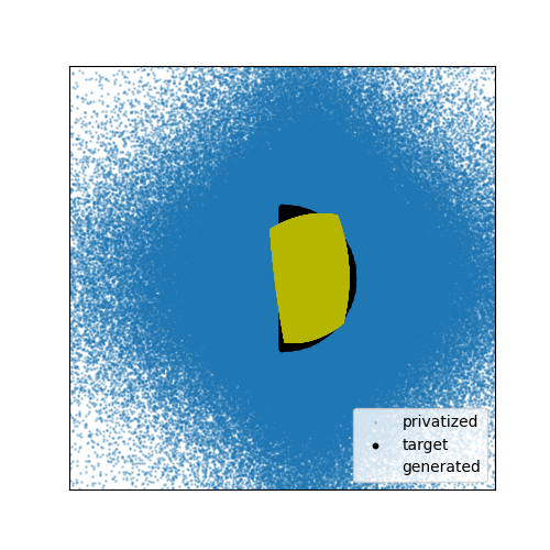
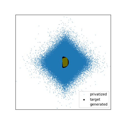
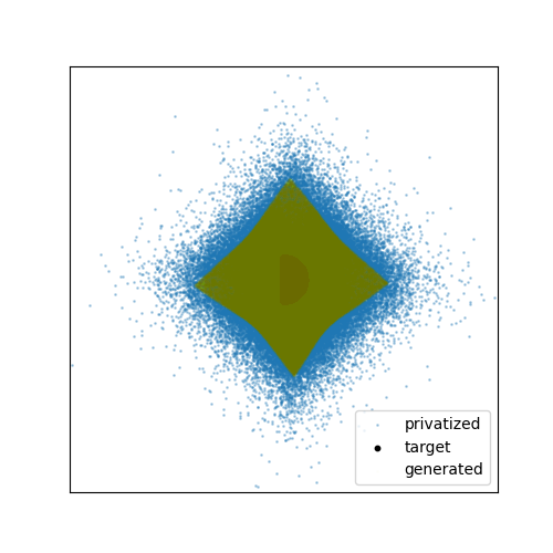
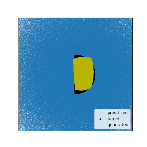
(a) entropic $p$-WGAN (9)

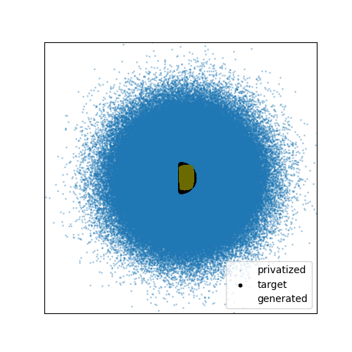
(b) entropic $p$-WGAN (9) (enlarged)

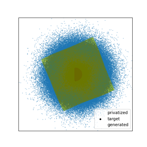
(c) unregularized $p$-WGAN (1)

Figure 1: Learning data from the half-circle manifold privatized with Laplace mechanism $\epsilon=5$ (top) and Gaussian mechanism $\epsilon=5,\delta=10^{-4}$ (bottom). Columns (a) and (b) show the manifold learned with entropic $p$-Wasserstein GAN (9), and column (c) shows the manifold learned with unregularized $p$-Wasserstein GAN (7). Note $p=1$ for Laplace mechanism and $p=2$ for Gaussian mechanism.

We note that the $\epsilon=5$ local differential privacy guarantee obtained with the Laplace mechanism can be translated to a central privacy guarantee by leveraging privacy amplification by shuffling. Since the distribution of the output of algorithm 1 does not depend on the order of the samples in the privatized data (due to the random sampling) and because the local privatization mechanism only depends on the data at the client and no auxiliary input, one can assume that the data is shuffled before privatization, which allows to apply [Feldman et al., 2023, Theorem 3.2], resulting in a $(\epsilon_{c}=0.353,\delta_{c}=10^{-6})$ central differential privacy guarantee for the Laplace mechanism.

4.3 MNIST: Comparison with wavelet denoising

We next provide our experimental results with MNIST LeCun [1998] and DCGAN Radford et al. [2015] generator. For the fair comparison, experiments in this section do not involve projecting onto the $\ell_{1}/\ell_{2}$ balls and the amximum radius of the ball where the images fall was used for sensitivity: since each pixel lies in $[-1,1],$ the maximum $\ell_{1}$ norm of the images is $28^{2}$ and the maximum $\ell_{2}$ norm is $28$. We use $100$-dimensional Uniform $[0,1]$ noise at the input to the generator ($\mathcal{P}_{z}=\text{Unif}[0,1]^{100}$). In Figure 2, we show two raw samples from the MNIST dataset (first column) and the corresponding privatized images (second column). In the third column, we denoise the privatized images in the second column with wavelet transform Mallat [1999]; the results indicate that the wavelet transform can not be used to recover the images. Here, the wavelet transform parameters for denoising (the wavelet basis, the level and reconstruction thresholds) were optimized to minimize the average distance between the reconstructed and original image under the particular noise instance, thus providing better results than one would expect in a fully privatized setting. We next show sampled images obtained by training GANs with $p$-Wasserstein loss (without entropic regularization) on privatized images (fourth column). The results indicate that GANs trained with Wasserstein loss without entropic regularization fail to learn from privatized data. In the fifth column, we train a Wasserstein-GAN Gulrajani et al. [2017] on the wavelet-denoised images, which also fails to provide useful samples. Finally, in the sixth column provide samples obtained by our method stated in algorithm 1 in Figure 2. For training the entropic $p$-WGAN we use the $400$ Sinkhorn-Knopp iterations and the Adam optimizer with learning rate $10^{-4}$ for $100$ epochs. No clipping of the norm of images was performed. Results with more sampled images and lower privacy regimes can be found in the supplementary material.

(a) original

(b) privatized

(c) wavelet
denoising

(d) $p$-WGAN (1)

(e) denoising
+$p$-WGAN

(f) Entropic $p$-WGAN (9)

Figure 2: Image samples privatized with Gaussian $(\epsilon,\delta)=(35,10^{-4})$ (top) and Laplace mechanism $\epsilon=196$ (bottom) and generated images from GANs trained on the data.

The results demonstrate that naive denoising with wavelet transform, which is a standard for image denoising, is unable to reconstruct the mnist images privatized with either Gaussian or Laplace noise at the chosen privatization level. Since the parameters for the wavelet transform were chosen based on the non-privatized images, we can think of wavelet denoising + p-WGAN as only approximately private at the same privacy level. In contrast, the entropic p-WGAN generator learned with the privatized samples was able to learn the distribution far beyond the values of $\epsilon$ needed for the wavelet transform reconstruction.

4.4 MNIST: Higher Privacy samples

In this section, we further investigate the performance of entropic $p$-Wasserstein GAN on locally privatized data. We set the number of sinkhorn steps $L=400$ and the batch size to be $b=400$ and we performed optimization with Adam optimizer Kingma and Ba [2014] and learning rate varied in $\{0.005,10^{-4},5\times 10^{-5}\}.$ We optimized for 150 epochs. For $p=1$ we first took the discrete cosine transform of the images and clipped the coefficients below 0.8 quantile to preserve more information, and then to control the sensitivity, we projected each training image onto an $\ell_{1}$ ball with radius $140$ (the parameters were chosen based on 1 held-out image in a way that it would not visually distort the image beyond recognition). We also applied DCT transform to the generator output before plugging it into the loss function. Similarly, for $p=2$ we projected each training image onto an $\ell_{2}$ ball with radius $20$, but we did not apply any transforms (since $\ell_{2}$-norm does not change under multiplication by an orthonormal matrix).

Figure 3: Entropic 1-WGAN on MNIST trained on data privatized with the Laplace mechanism achieving $\epsilon$-LDP $\epsilon=35$ (left) and $\epsilon=25$ (right)

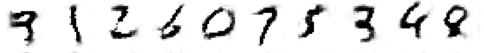
Figure 4: Entropic 2-WGAN on MNIST trained on data privatized with the Gaussian mechanism achieving $(\epsilon,\delta)$-LDP with $\delta=10^{-4}$ and $\epsilon=30$ (left) and $\epsilon=25$ (right)

The results indicate the effectiveness of our model at higher privacy regimes. However, smaller $\epsilon$ values still produced a lot of noise in the generated samples or eroded the images significantly. This can be potentially mitigated by increasing the number of samples as suggested in Theorem 2; however the relatively small size of MNIST limits the privacy levels that can be achieved. We discuss convergence in more detail in the next section.

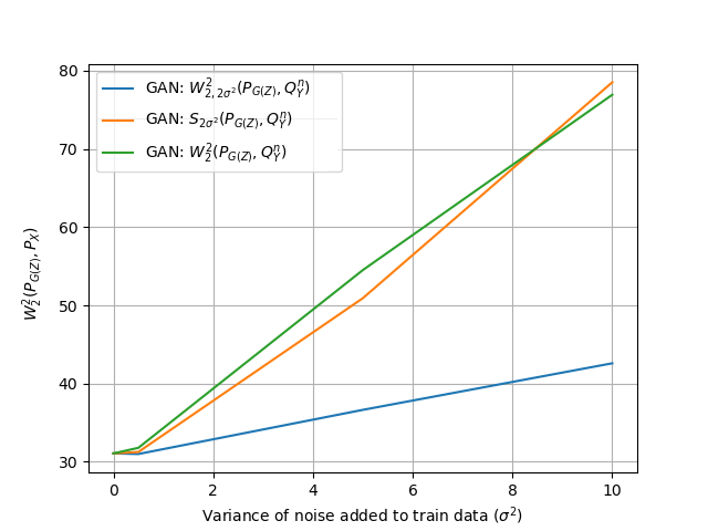
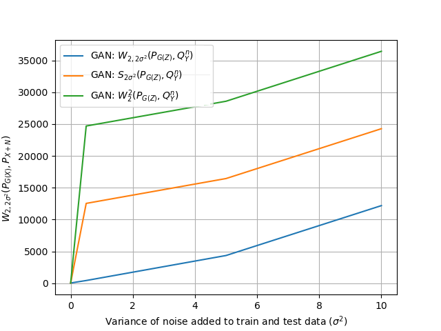
Figure 5: Dependence of the $2$-Wasserstein distance(left) and the validation error (right) on the noise scale $\sigma$

.

4.5 MNIST: Empirical convergence

We next empirically check how the performance (measured by the $2$-Wasserstein distance) depends on the privatization level. In our experiment, we set $p=2$ and train GANs on privatized MNIST samples with 3 different loss functions: the entropy-regularized 2-Wasserstein loss $W_{2,2\sigma^{2}}(P_{G(Z)},Q_{Y}^{n})$ (where $Q_{Y}^{n}$ represents the empirical distribution of the privatized samples), the 2-Wasserstein distance $W_{2}^{2}(P_{G(Z)},Q_{Y}^{n})$ and the sinkhorn divergence Feydy et al. [2019] (which is the debiased version of the entropy-regularized 2-Wasserstein distance). We chose a smaller generator model for this experiment – a 2 hidden layer fully connected neural network with 500 neurons on each hidden layer and a 2-dimensional latent distribution, i.e. $P_{Z}=\text{Uniform}[0,1]^{2},L=200,b=200.$ The images were then flattened into $28^{2}$-dimensional vectors. We report the $2$-Wasserstein distance between the generated and the target distribution $P_{X}$ in Figure 5 (left) where we approximate the target distribution by the empirical distribution of the non-privatized data. It is not surprising that the Wasserstein distance between the generated and the target distribution is smallest for the the entropy-regularized 2-Wasserstein GAN since our theory suggest that the entropic regularization encourages the generated distribution to converge to the (true) target distribution. The results also show that the distance grows with the noise scale $\sigma$ for all three of the metrics we considered, however, the slope of our method $W_{2,2\sigma^{2}}(P_{G(Z)},Q_{Y}^{n})$ is the smallest. The growth is to be expected from theorem 2, when the dataset size $n$ is kept constant, increasing the noise scale $\sigma$ (and thus privatization) degrades the performance. We also report the entropy-regularized 2-Wasserstein distance to the privatized dataset since it is minimized when $P_{G(Z)}=P_{X}$ and can be used as a measure of closeness of $P_{G(Z)}$ to $P_{X}.$ The plot indicates that the Sinkhorn divergence and the unregularized Wasserstein distance do not implicitly minimize this measure. We defer the results on the dependence of the error on the train set size to the supplementary material.

5 Appendix

We first prove the following lemma, which is used in the proof of Theorem 1 and Corollary 3.

Lemma 1.

Let $X\sim P_{X},G\sim P_{G}$ and $Y=M(X)=X+N,$ where $N=(N_{1},\ldots,N_{d})\sim f_{N}$ independent of $X$ and $f_{N}(x)=\frac{1}{C_{N}^{d}\sigma^{d}}e^{-\|x\|^{p}/(p\sigma^{p})}$ Then

$$D_{KL} (P_{Y}\|P_{G}*f_{N})\leq\frac{1}{2\sigma^{2}}\left(W_{2,2\sigma^{2}}(P_{Y},P_{G})-W_{2,2\sigma^{2}}(P_{Y},P_{X})\right),$$ (16)

where $D_{KL}(P\|Q)$ is the KL-divergence ($D_{KL}(P\|Q)=\int P(x)\log\frac{P(x)}{Q(x)}dx$ for continuous $P_{X}$ and $D_{KL}(P\|Q)=\sum_{x\in\mathcal{X}}P(x)\log\frac{P(x)}{Q(x)}$ for discrete $X$)

Proof.

By the formula for convolution: $P_{G}*f_{N}(x)=\int f_{N}(x-g)dP_{G}(g)=\mathbb{E}[f_{N}(x-G)].$ Note that $Y$ is a continuous random variable, and plugging its density $P_{Y}$ into the definition of KL-divergence we get:

$$D_{KL}(P_{Y}\|P_{G}*f_{N}) =\int\log\frac{P_{Y}(y)}{P_{G}*f_{N}(y)}P_{Y}(y)dy$$

$$=\mathbb{E}\log\frac{P_{Y}(Y)}{P_{G}*f_{N}(Y)}$$

$$=\mathbb{E}\log P_{Y}(Y)-\mathbb{E}\left[\log\left(\mathbb{E}[f_{N}(Y-G)\mid Y]\right)\right]$$

$$=-h(Y)-\mathbb{E}\left[\log\mathbb{E}[f_{N}(Y-G)\mid Y]\right].$$ (17)

The main ingredient for the rest of the proof will be the Donsker and Varadhan’s variational formula Donsker and Varadhan [1983]: for $U\sim P_{U}$ being a random variable supported on $\mathcal{U}$ and any measurable function $f:\mathcal{U}\to\mathbb{R},$ such that $\mathbb{E}[|f(U)|]<\infty,$ it holds that

$$\log\mathbb{E}_{U\sim P_{U}}\left[e^{f(U)}\right]=\sup_{P_{V}\ll P_{U}}\left\{\mathbb{E}_{V\sim P_{V}}[f(V)]-D_{KL}(P_{V}\|P_{U})\right\},$$ (18)

where $P_{V}\ll P_{U}$ indicates that $V$ is absolutely continuous with respect to $U.$

Now, we can use (18) to expand $\log\left(\mathbb{E}[f_{N}(Y-G)\mid Y=y]\right)$ in the negative term in (17). We fix some $y\in\mathbb{R}^{d}$ and choose $P_{U}:=P_{G}$ and $f(g):=f_{N}(y-g),$ then

$$\log\mathbb{E}[f_{N}(Y-G)\mid Y=y] =\log\mathbb{E}[f_{N}(y-G)]$$

$$=\sup_{P_{V}^{y}\ll P_{G}}\left\{\mathbb{E}_{V\sim P_{V}^{y}}[f_{N}(y-V)]-D_{KL}(P_{V}^{y}\|P_{G})\right\},$$

where we renamed $P_{V}$ into $P_{V}^{y}$ to emphasise its dependence on $y.$ Plugging the above into (17) produces:

$$D_{KL} (P_{Y}\|P_{G}*f_{N})=-h(P_{Y})-\mathbb{E}\left[\sup_{P_{V}^{y}\ll P_{G}}\mathbb{E}_{V\sim P_{V}^{y}}[\log f_{N}(Y-V)\mid Y]-D_{KL}(P_{V}^{y}\|P_{G})\right]$$

Denote now $\pi(v\mid y)=P_{V}^{y}(v)$ for any $v,y\in\mathbb{R}^{d}$ and notice that the supremum can be taken outside of the expectation since it is taken for each $y$ independently, which leads to

$$D_{KL} (P_{Y}\|P_{G}*f_{N})=-h(P_{Y})$$ (19)

$$-\sup_{\{\pi(v\mid y)\ll P_{G}\mid y\in\mathbb{R}^{d}\}}\mathbb{E}\left[\mathbb{E}_{V\sim\pi(\cdot\mid Y)}[\log f_{N}(Y-V)\mid Y]-D_{KL}(\pi(\cdot\mid Y)\|P_{G})\right].$$

Letting now $\mu(v)=\int\pi(v\mid y)P_{Y}(y)dy,$ we get that $\pi(v,y)=\pi(v\mid y)P_{Y}(y)$ is a coupling between $\mu$ and $P_{Y},$ i.e. $\pi\in\Pi(\mu,P_{Y}).$ Note that $\mu\ll P_{G}\iff\pi(v\mid y)\ll P_{G}$ since $P_{Y}(y)>0\forall y.$ Moreover, the supremum can be taken outside of the expectation since it is taken for each $y$ independently, which leads to

$$D_{KL} (P_{Y}\|P_{G}*f_{N})$$

$$=-\sup_{\mu\ll P_{G}}\sup_{\pi\in\Pi(\mu,P_{Y})}\mathbb{E}_{(V,Y)\sim\pi}\log f_{N}(Y-V)-\mathbb{E}D_{KL}(\pi(\cdot\mid Y)\|P_{G})-h(Y)$$

$$=\inf_{\mu\ll P_{G}}\inf_{\pi\in\Pi(\mu,P_{Y})}\mathbb{E}_{(V,Y)\sim\pi}[-\log f_{N}(Y-V)]+\mathbb{E}D_{KL}(\pi(\cdot\mid Y)\|P_{G})-h(Y)$$ (20)

As a final step we use the chain rule for KL-divergence: for any two joint distributions $Q^{1}\ll Q^{2}$ with marginals $(Q^{1}_{X},Q^{1}_{Y})$ and $(Q^{2}_{X},Q^{2}_{Y})$ correspondingly, it holds that

$$D_{KL}(Q^{1}\|Q^{2}) =D_{KL}(Q^{1}_{X}\|Q^{2}_{X})+\mathbb{E}_{X\sim Q^{1}_{X}}D_{KL}(Q^{1}(\cdot\mid X)\|Q^{2}(\cdot\mid X))$$ (21)

$$=D_{KL}(Q^{1}_{Y}\|Q^{2}_{Y})+\mathbb{E}_{Y\sim Q^{1}_{Y}}D_{KL}(Q^{1}(\cdot\mid Y)\|Q^{2}(\cdot\mid Y)).$$ (22)

Setting $Q^{1}=\pi$ and $Q^{2}=P_{G}\times P_{Y},$ we can rewrite the $D_{KL}$ term in (20) using (22) as

$$\mathbb{E}_{Y\sim P_{Y}}D_{KL}(\pi(\cdot\mid Y)\|P_{G}) =D_{KL}(\pi\|P_{G}\times P_{Y})-D_{KL}(\pi_{Y}\|P_{Y})$$

$$=D_{KL}(\pi\|P_{G}\times P_{Y})$$

$$=\mathbb{E}_{G\sim\mu}D_{KL}(\pi(\cdot\mid G)\|P_{Y})+D_{KL}(\mu\|P_{G}),$$ (23)

where in the last equality we used (21). For the first term in (24) we use (21) again with $Q^{1}=\pi$ and $Q^{2}=\mu\times P_{Y},$ which results in

$$\mathbb{E}D_{KL}(\pi(\cdot\mid Y)\|P_{G}) =\mathbb{E}_{G\sim\mu}D_{KL}(\pi\|\mu\times P_{Y})+D_{KL}(\mu\|P_{G})$$ (24)

We finally note that $I_{\pi}(G,Y)=D_{KL}(\pi\|\mu\times P_{Y})$ by the definition of mutual information. Plugging this and (24) into (20) gives

$$D_{KL} (P_{Y}\|P_{G}*f_{N})=$$

$$\inf_{\mu\ll P_{G}}\inf_{\pi\in\Pi(\mu,P_{G})}\mathbb{E}_{(V,Y)\sim\pi}[-\log f_{N}(Y-V)]+I_{\pi}(G,Y)+D_{KL}(\mu\|P_{G})-h(Y).$$

Letting $\mu=P_{G}$ gives us the upper bound:

$$D_{KL} (P_{Y}\|P_{G}*f_{N})$$

$$\leq\inf_{\pi\in\Pi(P_{G},P_{Y})}\mathbb{E}_{(G,Y)\sim\pi}[-\log f_{N}(Y-G)]+I_{\pi}(G,Y)-h(Y)$$

We can now plug in $f_{N}(x)=\frac{1}{C_{N}^{d}\sigma^{d}}e^{-\|x\|_{p}^{p}/\sigma^{p}p}:$

$$D_{KL} (P_{Y}\|P_{G}*f_{N})$$

$$\leq\inf_{\pi\in\Pi(P_{G},P_{Y})}\mathbb{E}_{(G,Y)\sim\pi}\left[\frac{\|Y-G\|_{P}^{P}}{p\sigma^{p}}\right]+I_{\pi}(G,Y)+d\log(C_{N}\sigma)-h(Y)$$

$$=\frac{1}{p\sigma^{p}}\left(W_{p,p\sigma^{p}}(P_{Y},P_{G})+dp\sigma^{p}\log(C_{N}\sigma)-p\sigma^{p}h(Y)\right)$$

$$=\frac{1}{p\sigma^{p}}\left(W_{p,p\sigma^{p}}(P_{Y},P_{G})-W_{p,p\sigma^{p}}(P_{Y},P_{X})\right),$$ (25)

where we used $W_{p,p\sigma^{p}}(P_{Y},P_{X})=p\sigma^{p}(h(Y)-d\log(C_{N}\sigma))$ from (15). ∎

5.1 Proof of Part (ii) of Theorem • ‣ 1

To show (11) we first prove that

$$W_{p,p\sigma^{p}}(P_{G(Z)},P_{Y})-W_{p,p\sigma^{p}}(P_{X},P_{Y})\leq W_{p}^{p}(P_{G(Z)},P_{X}).$$ (26)

We fix a coupling $\pi\in\Pi(P_{G(Z)},P_{X})$ and let $(G(Z),X)\sim\pi$ and $Y=X+N$ where $N\sim f_{N}$ is independent of $(X,G(Z)).$ Then

$$\mathbb{E}[\|{G(Z)}-Y\|_{p}^{p}]\leq\mathbb{E}[\|{G(Z)}-X\|_{p}^{p}]+\mathbb{E}[\|X-Y\|_{p}^{p}],$$ (27)

where for $p=1$ this is the triangle inequality and for $p=2:$

$$\mathbb{E}[\|{G(Z)}-Y\|_{2}^{2}] =\mathbb{E}[\|{G(Z)}-X\|_{2}^{2}]+2\mathbb{E}[({G(Z)}-X)^{T}(X-Y)+\mathbb{E}[\|X-Y\|_{2}^{2}]$$

$$=\mathbb{E}[\|{G(Z)}-X\|_{2}^{2}]+2\mathbb{E}[({G(Z)}-X)^{T}N]+\mathbb{E}[\|X-Y\|_{2}^{2}].$$

By the independence of $N$ and $G(Z),X:$

$$\mathbb{E}[({G(Z)}-X)^{T}N]=\mathbb{E}[({G(Z)}-X)]^{T}\mathbb{E}[N]=0$$

since $\mathbb{E}[Y-X]=\mathbb{E}[N]=0.$ So, (27) holds for $p=2$ as well as for $p=1.$ Also note that $G(Z)-X-Y$ forms a Markov chain, so the data processing inequality holds:

$$I(G(Z),Y)\leq I(X,Y).$$

Thus, for any $\pi\in\Pi(P_{G(Z)},P_{X})$ and for $Y=X+N$ with $N$ independent of $G(Z),X:$

$$\mathbb{E}[G(Z)-Y\|_{p}^{p}]+p\sigma^{p}I(G(Z),Y)\leq\mathbb{E}[\|G(Z)-X\|_{p}^{p}]+\mathbb{E}[\|X-Y\|_{p}^{p}]+p\sigma^{p}I(X,Y)$$

Note that the infimum of the LHS over all couplings $\pi^{\prime}\in\Pi(P_{G(Z)},P_{Y})$ is by definition (8) $W_{p,p\sigma^{p}}(P_{G(Z)},P_{Y}).$ So, for any $\pi\in\Pi(P_{G(Z)},P_{X}):$

$$W_{p,p\sigma^{p}}(P_{G(Z)},P_{Y}) \leq\mathbb{E}_{(G(Z),X)\sim\pi}[\|{G(Z)}-X\|_{p}^{p}]+\mathbb{E}[\|X-Y\|_{p}^{p}]+p\sigma^{p}I_{\pi}(X,Y)$$

Now taking the infimum over $\pi\in\Pi(P_{G(Z)},P_{X})$ on the RHS and recalling that

$$\inf_{\pi\in\Pi(P_{G(Z)},P_{X})}\mathbb{E}_{\pi}[\|{X}-G(Z)\|_{p}^{p}]=W_{p}^{p}(P_{G(Z)},P_{X}),$$

leads to

$$W_{p,p\sigma^{p}}(P_{G(Z)},P_{Y}) \leq W_{p}^{p}(P_{G(Z)},P_{X})+\mathbb{E}[\|X-Y\|_{p}^{p}]+p\sigma^{p}I_{\pi}(X,Y)$$

The only thing left to show is that

$$\mathbb{E}[\|X-Y\|_{p}^{p}]+p\sigma^{p}I_{\pi}(X,Y)=W_{p,p\sigma^{p}}(P_{X},P_{Y}),$$

but this follows from our choice of $Y=X+N$ and part (i) of Theorem • ‣ 1.

Second, we show that

$$W_{p,p\sigma^{p}}(P_{G(Z)},P_{Y})-W_{p,p\sigma^{p}}(P_{X},P_{Y})\geq D_{KL}(P_{G(Z)+N},P_{X+N}).$$

It follows directly from Lemma 1 by setting $G=G(Z).$ Combining this with (26) results in

$$D_{KL}(P_{G(Z)+N},P_{X+N})\leq W_{p,p\sigma^{p}}(P_{G(Z)},P_{Y})-W_{p,p\sigma^{p}}(P_{X},P_{Y})\leq W_{p}^{p}(P_{G(Z)},P_{X})$$

Letting

$$G^{*}=\arg\min_{G\in\mathcal{G}}W_{p,p\sigma^{p}}(P_{G(Z)},P_{Y}),$$

and taking the minimum on both sides of

$$W_{p,p\sigma^{p}}(P_{G(Z)},P_{Y})-W_{p,p\sigma^{p}}(P_{X},P_{Y})\leq W_{p}^{p}(P_{G(Z)},P_{X})$$

leads to

$$D_{KL}(P_{G^{*}(Z)+N},P_{X+N})\leq W_{p,p\sigma^{p}}(P_{G^{*}(Z)},P_{Y})-W_{p,p\sigma^{p}}(P_{X},P_{Y})\leq\min_{G\in\mathcal{G}}W_{p}^{p}(P_{G(Z)},P_{X}).$$

5.2 Proof of Theorem 2 and Corollary 3

Theorem 2 follows from the following theorem proved in [Reshetova et al., 2021, Theorem 6].

Theorem 3.

[Reshetova et al., 2021, Theorem 6]

Let ${P}_{Z}$ and ${P}_{Y}$ be sub-Gaussian and the set of generators $\mathcal{G}$ consist of $L$-Lipschitz functions, i.e. $\|G(Z_{1})-G(Z_{2})\|\leq L\|Z_{1}-Z_{2}\|$ for any $Z_{1},Z_{2}$ in the support of $P_{Z}$ and let $\mathcal{G}$ satisfy (12). Then the generalization error for entropic GAN with $p=2$ (9) can be both upper bounded as

$$\mathbb{E}\bigl{[}W_{2,\lambda}^{2}({P}_{G^{n}(Z)},{P}_{Y})-W_{2,\lambda}^{2}({P}_{G^{*}(Z)},{P}_{Y})\bigr{]}\leq C_{d}\lambda n^{-1/2}\bigl{(}1+(2\tau^{2}/\lambda)^{\lceil 5d/4\rceil+3}\bigr{)}$$ (28)

with $\tau^{2}=\max\{L^{2}\sigma^{2}(Z),\sigma^{2}(Y)\}$.

We present the proof of Theorem 2 below:

Proof.

In our case $\lambda=2\sigma^{2}$ and $Y=X+N$ with $N\sim\mathcal{N}(0,\sigma^{2}I),$ so $\sigma(Y)\leq\sigma(X)+\sigma(N),$ where $\sigma(N)=\sigma^{2}.$ Thus, plugging it into the theorem we get

$$\mathbb{E}\bigl{[}W_{2,\lambda}^{2}({P}_{G^{n}(Z)},{P}_{Y})-W_{2,\lambda}^{2} ({P}_{G^{*}(Z)},{P}_{Y})\bigr{]}$$

$$\leq C_{d}\sigma^{2}n^{-1/2}\left(1+\left(\frac{\max\{L\sigma(Z),\sigma(X)+\sigma\}}{\sigma}\right)^{2\lceil\frac{5d}{4}\rceil+6}\right)$$

Letting $\tau=\max\{L\sigma(Z)/\sigma(X),1\}$ we get $(\sigma(X)+\sigma)\tau\geq\max\{L\sigma(Z),\sigma(X)+\sigma\},$ which leads to

$$\mathbb{E}\bigl{[}W_{2,\lambda}^{2}({P}_{G^{n}(Z)},{P}_{Y})-W_{2,\lambda}^{2} ({P}_{G^{*}(Z)},{P}_{Y})\bigr{]}$$

$$\leq C_{d}\sigma^{2}n^{-1/2}\left(1+\left(\tau^{2}\left(1+\sigma(X)/\sigma\right)^{2}\right)^{\lceil\frac{5d}{4}\rceil+3}\right).$$

∎

We can now prove Corollary 3.

Proof.

Denoting $f_{N}$ the pdf of $\mathcal{N}(0,\sigma^{2}I)$ and plugging it into lemma 1 with $P_{G}=P_{G^{n}(Z)}$ leads to

$$D_{KL}(P_{Y}\|P_{G^{n}(Z)}*f_{N}) \leq\frac{1}{2\sigma^{2}}\left(W_{2,2\sigma^{2}}(P_{Y},P_{G^{n}(Z)})-W_{2,2\sigma^{2}}(P_{Y},P_{X})\right).$$

Taking the expectation of both sides and applying Theorem 2 proves the claim. ∎

5.3 Additional Experiments

5.3.1 Additional Experiments with synthetic data

In figures 6 and 7 we provide additional results for section 4.2 for ellipsis and rectangular-shaped manifolds for Laplace mechanism in figure 6 and Gaussian mechanism in figure 7.

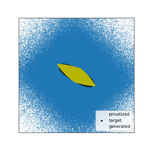
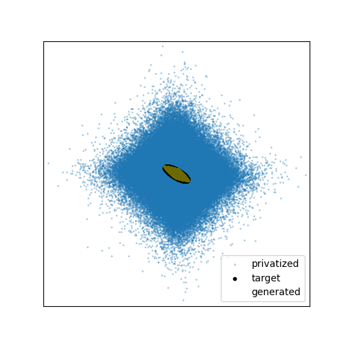
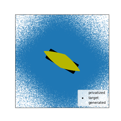
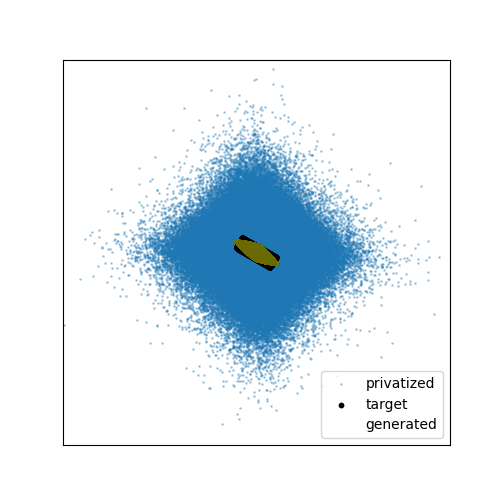
Figure 6: Learning data from the ellipsis (top) and rectangular-shaped (bottom) manifolds privatized with Laplace mechanism $\epsilon=5$ and entropic $1$-Wasserstein GAN (9) . Right plot is the upscaled version of the left one.

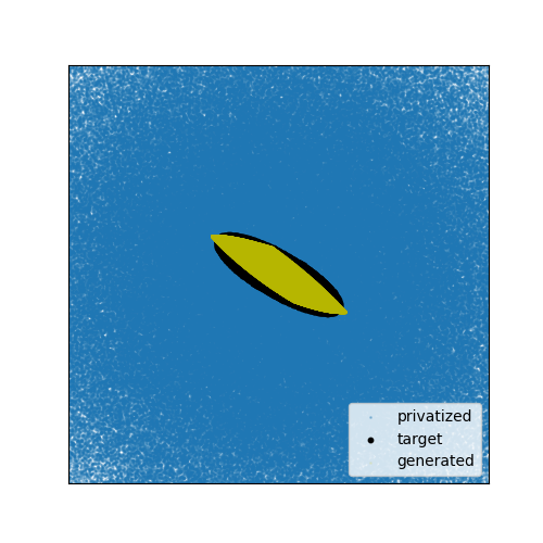
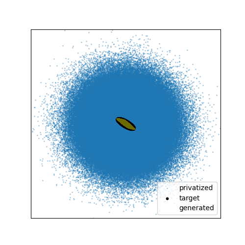
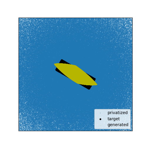
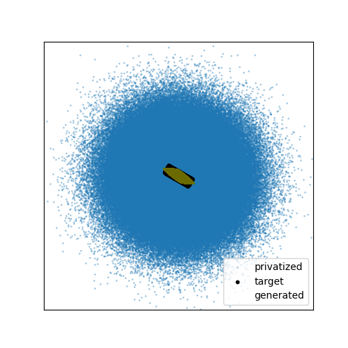
Figure 7: Learning data from the ellipsis (top) and rectangular-shaped (bottom) manifolds privatized with Gaussian mechanism $\epsilon=5,\delta=10^{-4}$ and entropic $2$-Wasserstein GAN (9). Right plot is the upscaled version of the left one.

5.3.2 Additional samples for comparing wavelet transform, GAN with no regularization and with entropic regularization

In Figure 8 we provide 200 uniformly random samples for Entropic $p$-WGAN on MNIST trained on data privatized with the corresponding mechanism together with the privace parameter. The setting of the experiment is the same as in section 4.5.

$\epsilon=1568$

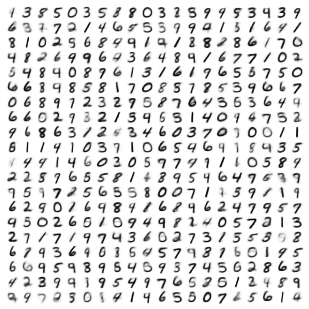
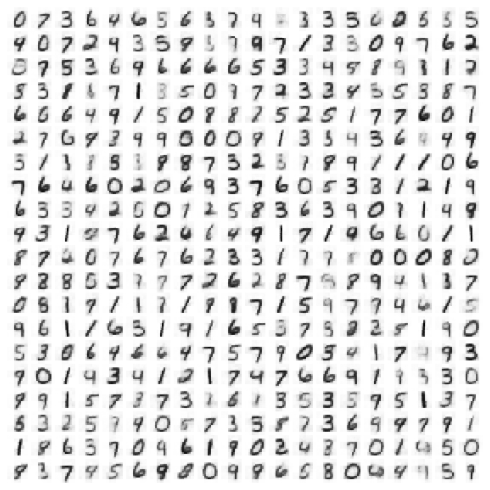
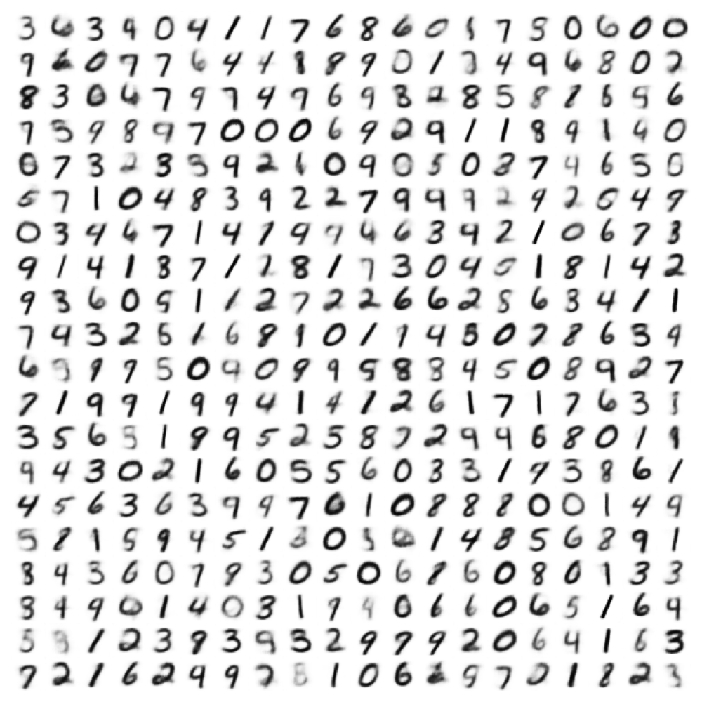
$\epsilon=196$

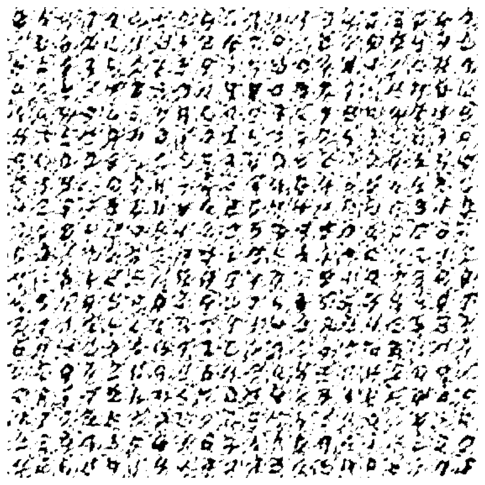
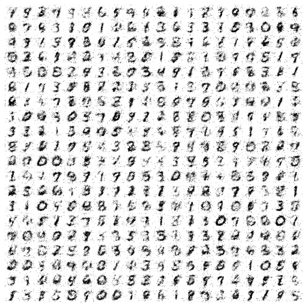
$\epsilon=1568,\delta=10^{-4}$

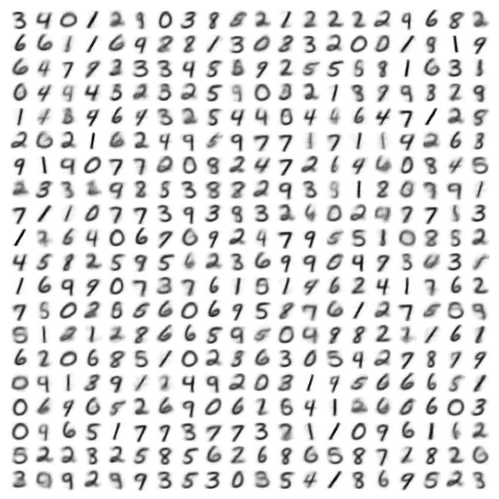
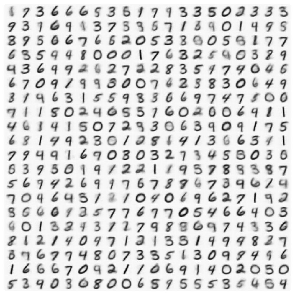
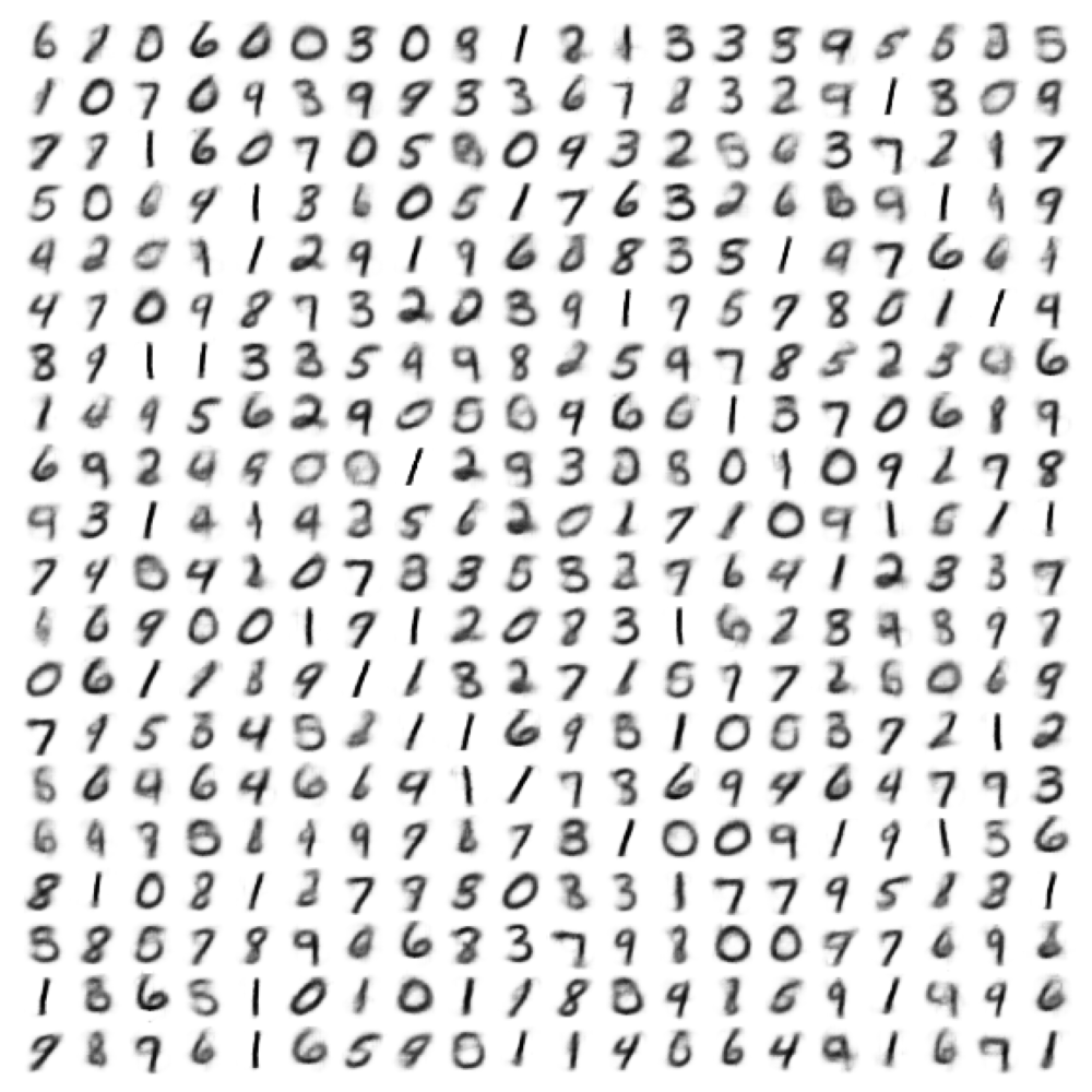
$\epsilon=41,\delta=10^{-4}$

(a) $p$-WGAN 6

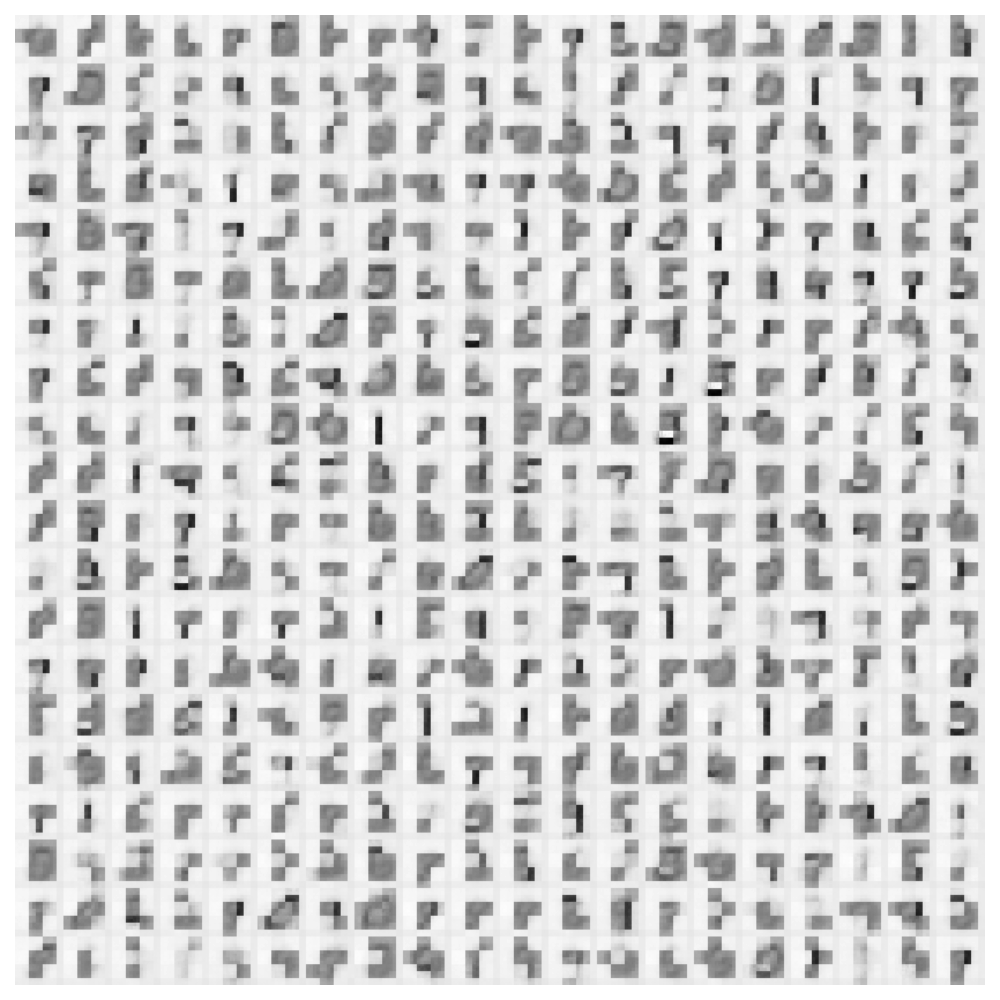
(b) Wavelet denoising+$p$-WGAN

(c) $p$-EWGAN 7

Figure 8: Comparing Wavelet denoising and Entropic p-WGAN for $p=1$ and Laplace mechanism (top 2 rows) and $p=2$ and Gaussian mechanism (bottom 2 rows)

5.4 Additional Experiments for higher privacy samples

In this section we provide additional results for section 4.4 with different privacy levels and report 400 randomly sampled digits on figure 9 for the Laplace mechanism and on figure 10 for Gaussian mechanism.

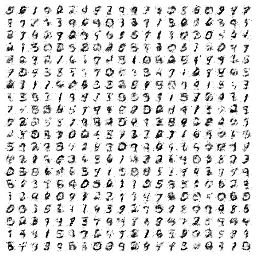
(a) $\epsilon=65.25$

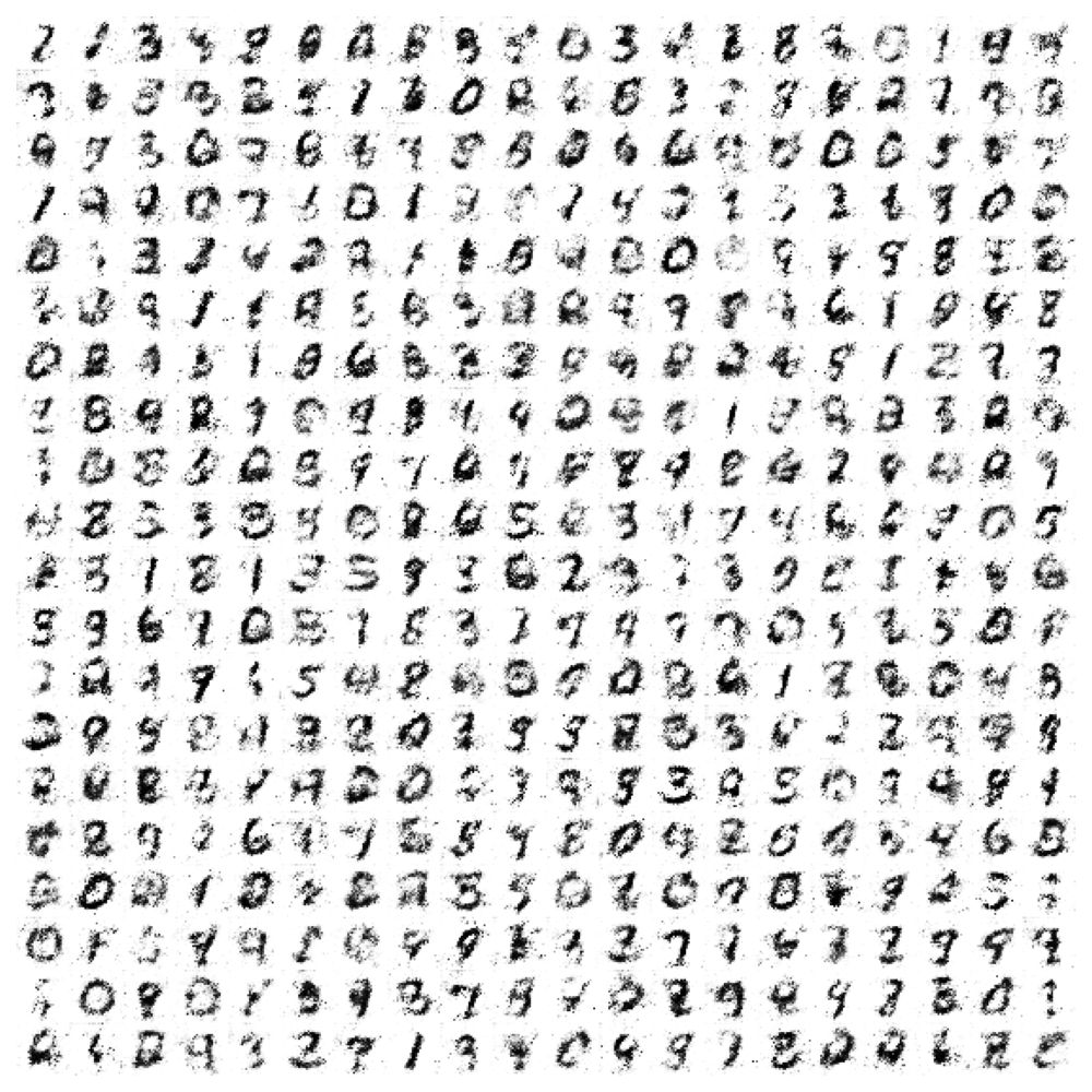
(b) $\epsilon=49$

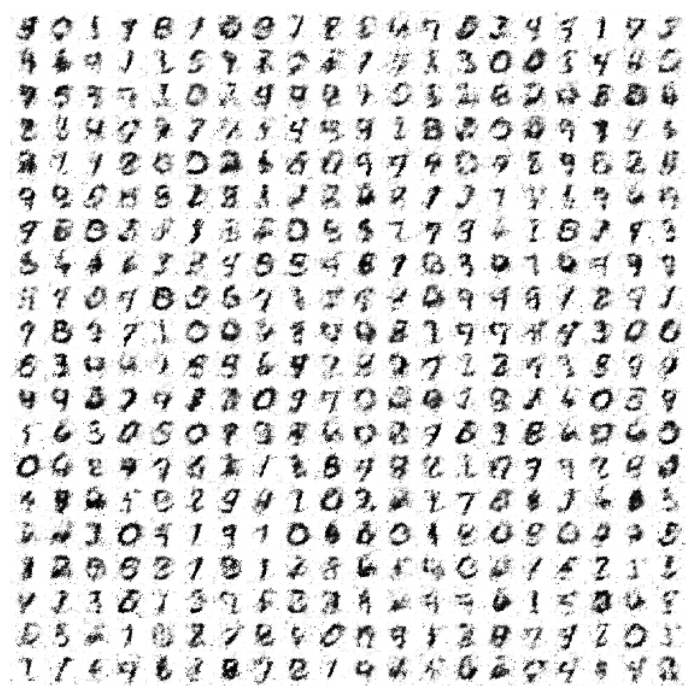
(c) $\epsilon=35$

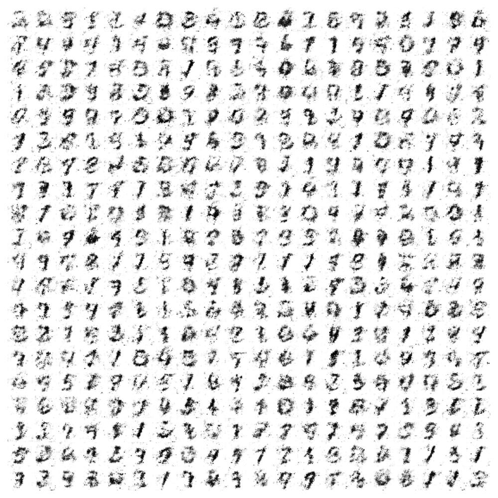
(d) $\epsilon=25$

Figure 9: Laplace mechanism with different privacy budgets $\epsilon$ and clipping of the discrete cosine transform, 1-EWGAN

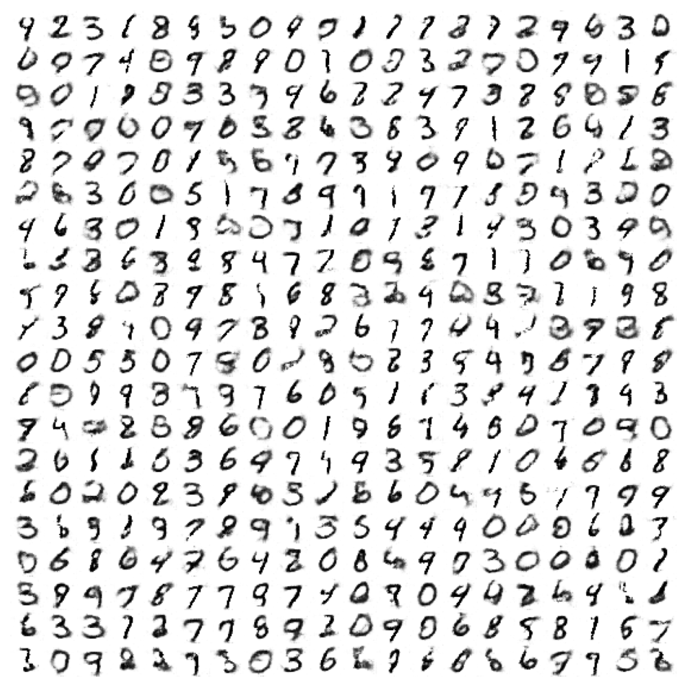
(a) $\epsilon=35$

(b) $\epsilon=30$

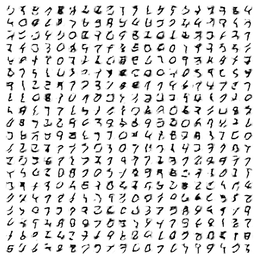
(c) $\epsilon=25$

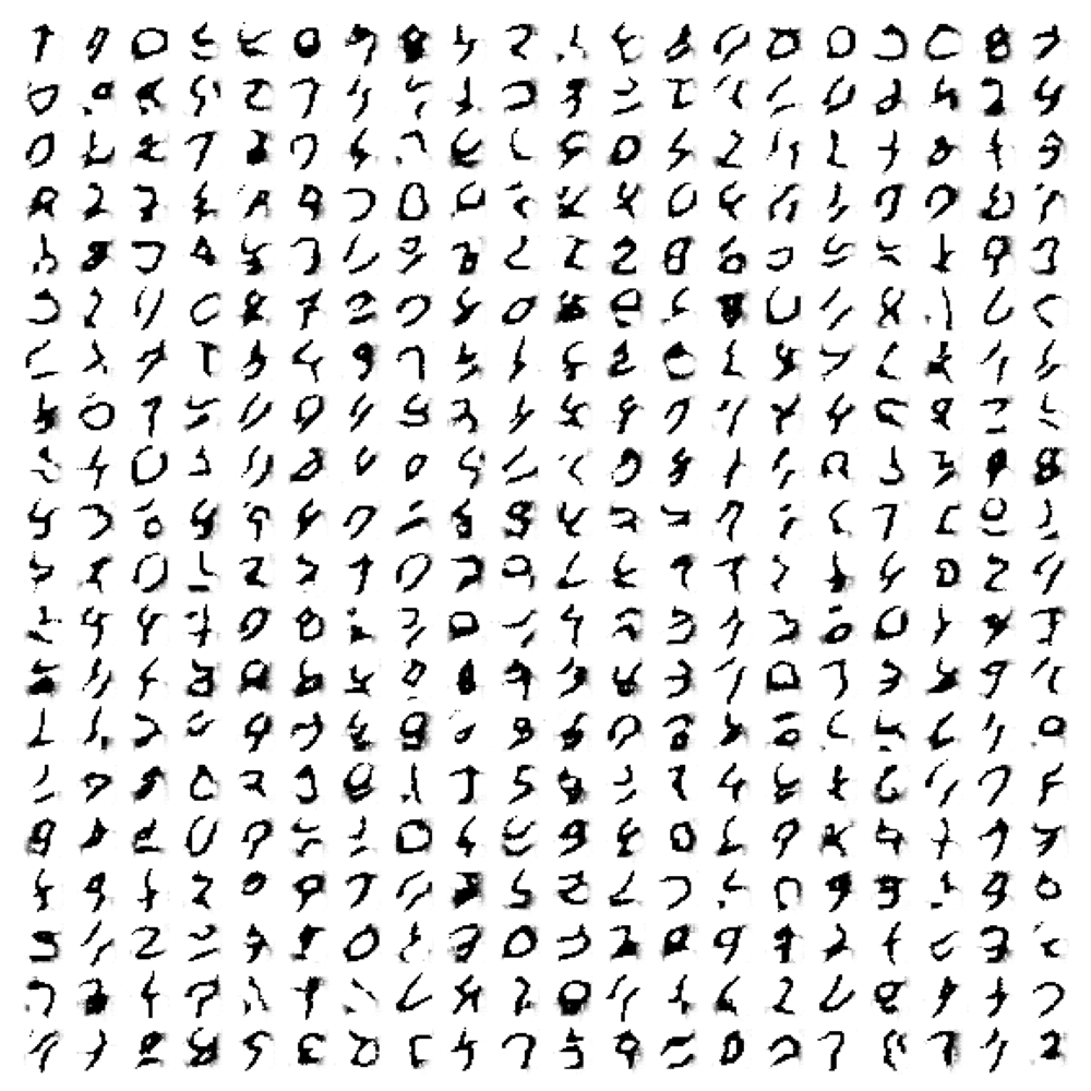
(d) $\epsilon=24$

Figure 10: Gaussian mechanism with different privacy budgets $\epsilon$ and clipping the euclidean norm of images, 2-EWGAN

5.5 Influence of train set size on the error

Here we empirically check how the performance (measured by the $2$-Wasserstein distance) depends on the size of the training set . We use the setting described in section 4.5 with $\sigma^{2}=4$ and train the model with the entropy-regularized 2-Wasserstein loss between the generated distribution and the empirical distribution of the privatized samples $W_{2,2\sigma^{2}}(P_{G(Z)},Q_{Y}^{n}).$ We report the $2$-Wasserstein distance between the generated $P_{G(Z)}$ and the target distribution $P_{X}$ on Figure 11, where we approximate the target distribution by the empirical distribution of the non-privatized data that was used for training (curve labeled "train") and that was left out for validation (curve labeled "test"). To compute $W_{2,2\sigma^{2}}(P_{G(Z)},P_{Y})$ we use mini-batches of size $200.$ The distance is decreasing on the left plot for both train and test curves, which is expected by theorem 2 to be proportional to $1/\sqrt{n}.$ The closeness of the train and test curves also shows no signs of overfitting, which is most probably happening due to privatization.

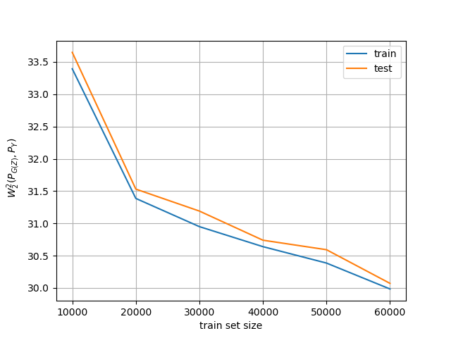
Figure 11: Dependence of $W_{2,2\sigma^{2}}(P_{G(Z)},P_{Y})$ on the dataset size $n$

References

- Dwork et al. [2006a] Cynthia Dwork, Frank McSherry, Kobbi Nissim, and Adam Smith. Calibrating noise to sensitivity in private data analysis. In Theory of Cryptography: Third Theory of Cryptography Conference, TCC 2006, New York, NY, USA, March 4-7, 2006. Proceedings 3, pages 265–284. Springer, 2006a.
- Kasiviswanathan et al. [2011] Shiva Prasad Kasiviswanathan, Homin K Lee, Kobbi Nissim, Sofya Raskhodnikova, and Adam Smith. What can we learn privately? SIAM Journal on Computing, 40(3):793–826, 2011.
- De et al. [2016] Abir De, Isabel Valera, Niloy Ganguly, Sourangshu Bhattacharya, and Manuel Gomez Rodriguez. Learning and forecasting opinion dynamics in social networks. In Advances in Neural Information Processing Systems, volume 29, pages 397–405. Curran Associates, Inc., 2016.
- Isola et al. [2017] Phillip Isola, Jun-Yan Zhu, Tinghui Zhou, and Alexei A Efros. Image-to-image translation with conditional adversarial networks. In Proceedings of the IEEE conference on computer vision and pattern recognition, pages 1125–1134, 2017.
- Reed et al. [2016] Scott Reed, Zeynep Akata, Xinchen Yan, Lajanugen Logeswaran, Bernt Schiele, and Honglak Lee. Generative adversarial text to image synthesis. arXiv preprint arXiv:1605.05396, 2016.
- Ledig et al. [2017] Christian Ledig, Lucas Theis, Ferenc Huszár, Jose Caballero, Andrew Cunningham, Alejandro Acosta, Andrew Aitken, Alykhan Tejani, Johannes Totz, Zehan Wang, et al. Photo-realistic single image super-resolution using a generative adversarial network. In Proceedings of the IEEE conference on computer vision and pattern recognition, pages 4681–4690, 2017.
- Feizi et al. [2020] Soheil Feizi, Farzan Farnia, Tony Ginart, and David Tse. Understanding gans in the lqg setting: Formulation, generalization and stability. IEEE Journal on Selected Areas in Information Theory, 1(1):304–311, 2020.
- Flamary et al. [2021] Rémi Flamary, Nicolas Courty, Alexandre Gramfort, Mokhtar Z. Alaya, Aurélie Boisbunon, Stanislas Chambon, Laetitia Chapel, Adrien Corenflos, Kilian Fatras, Nemo Fournier, Léo Gautheron, Nathalie T.H. Gayraud, Hicham Janati, Alain Rakotomamonjy, Ievgen Redko, Antoine Rolet, Antony Schutz, Vivien Seguy, Danica J. Sutherland, Romain Tavenard, Alexander Tong, and Titouan Vayer. Pot: Python optimal transport. Journal of Machine Learning Research, 22(78):1–8, 2021. URL http://jmlr.org/papers/v22/20-451.html.
- Feydy et al. [2019] Jean Feydy, Thibault Séjourné, François-Xavier Vialard, Shun-ichi Amari, Alain Trouvé, and Gabriel Peyré. Interpolating between optimal transport and mmd using sinkhorn divergences. In The 22nd International Conference on Artificial Intelligence and Statistics, pages 2681–2690. PMLR, 2019.
- Song et al. [2013] Shuang Song, Kamalika Chaudhuri, and Anand D Sarwate. Stochastic gradient descent with differentially private updates. In 2013 IEEE global conference on signal and information processing, pages 245–248. IEEE, 2013.
- Chen et al. [2020a] Dingfan Chen, Tribhuvanesh Orekondy, and Mario Fritz. Gs-wgan: A gradient-sanitized approach for learning differentially private generators. Advances in Neural Information Processing Systems, 33:12673–12684, 2020a.
- Cao et al. [2021] Tianshi Cao, Alex Bie, Arash Vahdat, Sanja Fidler, and Karsten Kreis. Don’t generate me: Training differentially private generative models with sinkhorn divergence. Advances in Neural Information Processing Systems, 34:12480–12492, 2021.
- Xie et al. [2018] Liyang Xie, Kaixiang Lin, Shu Wang, Fei Wang, and Jiayu Zhou. Differentially private generative adversarial network. arXiv preprint arXiv:1802.06739, 2018.
- Zhang et al. [2018] Xinyang Zhang, Shouling Ji, and Ting Wang. Differentially private releasing via deep generative model (technical report). arXiv preprint arXiv:1801.01594, 2018.
- Papernot et al. [2018] Nicolas Papernot, Shuang Song, Ilya Mironov, Ananth Raghunathan, Kunal Talwar, and Úlfar Erlingsson. Scalable private learning with pate. arXiv preprint arXiv:1802.08908, 2018.
- Papernot et al. [2016] Nicolas Papernot, Martín Abadi, Ulfar Erlingsson, Ian Goodfellow, and Kunal Talwar. Semi-supervised knowledge transfer for deep learning from private training data. arXiv preprint arXiv:1610.05755, 2016.
- Seguy et al. [2017] Vivien Seguy, Bharath Bhushan Damodaran, Rémi Flamary, Nicolas Courty, Antoine Rolet, and Mathieu Blondel. Large-scale optimal transport and mapping estimation. arXiv preprint arXiv:1711.02283, 2017.
- Bassily et al. [2017] Raef Bassily, Kobbi Nissim, Uri Stemmer, and Abhradeep Guha Thakurta. Practical locally private heavy hitters. Advances in Neural Information Processing Systems, 30, 2017.
- Bun et al. [2019] Mark Bun, Jelani Nelson, and Uri Stemmer. Heavy hitters and the structure of local privacy. ACM Transactions on Algorithms (TALG), 15(4):1–40, 2019.
- Chen et al. [2021] Wei-Ning Chen, Peter Kairouz, and Ayfer Ozgur. Breaking the dimension dependence in sparse distribution estimation under communication constraints. In Conference on Learning Theory, pages 1028–1059. PMLR, 2021.
- Chen et al. [2020b] Wei-Ning Chen, Peter Kairouz, and Ayfer Ozgur. Breaking the communication-privacy-accuracy trilemma. Advances in Neural Information Processing Systems, 33:3312–3324, 2020b.
- Suresh et al. [2017] Ananda Theertha Suresh, X Yu Felix, Sanjiv Kumar, and H Brendan McMahan. Distributed mean estimation with limited communication. In International conference on machine learning, pages 3329–3337. PMLR, 2017.
- Bhowmick et al. [2018] Abhishek Bhowmick, John Duchi, Julien Freudiger, Gaurav Kapoor, and Ryan Rogers. Protection against reconstruction and its applications in private federated learning. arXiv preprint arXiv:1812.00984, 2018.
- Han et al. [2018] Yanjun Han, Pritam Mukherjee, Ayfer Ozgur, and Tsachy Weissman. Distributed statistical estimation of high-dimensional and nonparametric distributions. In 2018 IEEE International Symposium on Information Theory (ISIT), pages 506–510. IEEE, 2018.
- Arjovsky and Bottou [2017] Martin Arjovsky and Léon Bottou. Towards principled methods for training generative adversarial networks. arXiv preprint arXiv:1701.04862, 2017.
- Mescheder et al. [2018] Lars Mescheder, Andreas Geiger, and Sebastian Nowozin. Which training methods for gans do actually converge? In International conference on machine learning, pages 3481–3490. PMLR, 2018.
- Chaudhuri and Vinterbo [2013] Kamalika Chaudhuri and Staal A Vinterbo. A stability-based validation procedure for differentially private machine learning. In C.J. Burges, L. Bottou, M. Welling, Z. Ghahramani, and K.Q. Weinberger, editors, Advances in Neural Information Processing Systems, volume 26. Curran Associates, Inc., 2013. URL https://proceedings.neurips.cc/paper_files/paper/2013/file/e6d8545daa42d5ced125a4bf747b3688-Paper.pdf.
- Mansbridge et al. [2020] Alex Mansbridge, Gregory Barbour, Davide Piras, Christopher Frye, Ilya Feige, and David Barber. Learning to noise: Application-agnostic data sharing with local differential privacy. arXiv preprint arXiv:2010.12464, 2020.
- Warner [1965] Stanley L Warner. Randomized response: A survey technique for eliminating evasive answer bias. Journal of the American Statistical Association, 60(309):63–69, 1965.
- Evfimievski et al. [2003] Alexandre Evfimievski, Johannes Gehrke, and Ramakrishnan Srikant. Limiting privacy breaches in privacy preserving data mining. In Proceedings of the twenty-second ACM SIGMOD-SIGACT-SIGART symposium on Principles of database systems, pages 211–222, 2003.
- Dwork et al. [2006b] Cynthia Dwork, Krishnaram Kenthapadi, Frank McSherry, Ilya Mironov, and Moni Naor. Our data, ourselves: Privacy via distributed noise generation. In Advances in Cryptology-EUROCRYPT 2006: 24th Annual International Conference on the Theory and Applications of Cryptographic Techniques, St. Petersburg, Russia, May 28-June 1, 2006. Proceedings 25, pages 486–503. Springer, 2006b.
- Dwork et al. [2014] Cynthia Dwork, Aaron Roth, et al. The algorithmic foundations of differential privacy. Foundations and Trends® in Theoretical Computer Science, 9(3–4):211–407, 2014.
- Zhao et al. [2019] Jun Zhao, Teng Wang, Tao Bai, Kwok-Yan Lam, Zhiying Xu, Shuyu Shi, Xuebin Ren, Xinyu Yang, Yang Liu, and Han Yu. Reviewing and improving the gaussian mechanism for differential privacy. arXiv preprint arXiv:1911.12060, 2019.
- Peyré et al. [2019] Gabriel Peyré, Marco Cuturi, et al. Computational optimal transport: With applications to data science. Foundations and Trends® in Machine Learning, 11(5-6):355–607, 2019.
- Arjovsky et al. [2017] Martin Arjovsky, Soumith Chintala, and Léon Bottou. Wasserstein generative adversarial networks. In International conference on machine learning, pages 214–223. PMLR, 2017.
- Korotin et al. [2019] Alexander Korotin, Vage Egiazarian, Arip Asadulaev, Alexander Safin, and Evgeny Burnaev. Wasserstein-2 generative networks. arXiv preprint arXiv:1909.13082, 2019.
- Goldfeld et al. [2020] Ziv Goldfeld, Kristjan Greenewald, Jonathan Niles-Weed, and Yury Polyanskiy. Convergence of smoothed empirical measures with applications to entropy estimation. IEEE Transactions on Information Theory, 66(7):4368–4391, 2020.
- Reshetova et al. [2021] Daria Reshetova, Yikun Bai, Xiugang Wu, and Ayfer Özgür. Understanding entropic regularization in gans. In 2021 IEEE International Symposium on Information Theory (ISIT), pages 825–830. IEEE, 2021.
- Genevay et al. [2018] Aude Genevay, Gabriel Peyré, and Marco Cuturi. Learning generative models with sinkhorn divergences. In International Conference on Artificial Intelligence and Statistics, pages 1608–1617. PMLR, 2018.
- LeCun [1998] Yann LeCun. The mnist database of handwritten digits. http://yann. lecun. com/exdb/mnist/, 1998.
- Radford et al. [2015] Alec Radford, Luke Metz, and Soumith Chintala. Unsupervised representation learning with deep convolutional generative adversarial networks. arXiv preprint arXiv:1511.06434, 2015.
- Feldman et al. [2023] Vitaly Feldman, Audra McMillan, and Kunal Talwar. Stronger privacy amplification by shuffling for rényi and approximate differential privacy. In Proceedings of the 2023 Annual ACM-SIAM Symposium on Discrete Algorithms (SODA), pages 4966–4981. SIAM, 2023.
- Mallat [1999] Stéphane Mallat. A wavelet tour of signal processing. Elsevier, 1999.
- Gulrajani et al. [2017] Ishaan Gulrajani, Faruk Ahmed, Martin Arjovsky, Vincent Dumoulin, and Aaron Courville. Improved training of wasserstein gans. In Proceedings of the 31st International Conference on Neural Information Processing Systems, pages 5769–5779, 2017.
- Kingma and Ba [2014] Diederik P Kingma and Jimmy Ba. Adam: A method for stochastic optimization. arXiv preprint arXiv:1412.6980, 2014.
- Donsker and Varadhan [1983] Monroe D Donsker and SR Srinivasa Varadhan. Asymptotic evaluation of certain markov process expectations for large time. iv. Communications on pure and applied mathematics, 36(2):183–212, 1983.