Fast Sample Size Determination for Bayesian Equivalence Tests

Abstract

Equivalence testing allows one to conclude that two characteristics are practically equivalent. We propose a framework for fast sample size determination with Bayesian equivalence tests facilitated via posterior probabilities. We assume that data are generated using statistical models with fixed parameters for the purposes of sample size determination. Our framework defines a distribution for the sample size that controls the length of posterior highest density intervals, where targets for the interval length are calibrated to yield desired power for the equivalence test. We prove the normality of the limiting distribution for the sample size and introduce a two-stage approach for estimating this distribution in the nonlimiting case. This approach is much faster than traditional power calculations for Bayesian equivalence tests, and it requires users to make fewer choices than traditional simulation-based methods for Bayesian sample size determination.

Keywords: Experimental design; interval-based sample size determination; power analysis; practical equivalence; the Bernstein-von Mises theorem

1 Introduction

1.1 Two-Group Equivalence Tests

Equivalence testing (Spiegelhalter et al., 1994; Wellek, 2010; Walker and Nowacki, 2011) allows practitioners to account for practical equivalence when comparing scalar quantities $\theta_{1}$ and $\theta_{2}$, where the characteristic $\theta_{j}$ describes a comparison ($j=1$) or reference ($j=2$) group. These comparisons are typically facilitated using the difference between the characteristics: $\theta_{1}-\theta_{2}$. Equivalence testing defines an equivalence margin $\delta>0$, which is the smallest difference between $\theta_{1}$ and $\theta_{2}$ that is of practical importance. The corresponding interval $(-\delta,\delta)$ is a region of practical equivalence (ROPE) that reflects a continuum of differences that are small enough to be considered practically negligible.

Several Bayesian methods for equivalence testing exist. Morey and Rouder (2011) proposed the nonoverlapping hypotheses approach, which uses Bayes factors to compare the complementary hypotheses $H_{0}:\theta_{1}-\theta_{2}\in(-\delta,\delta)$ and $H_{1}:\theta_{1}-\theta_{2}\notin(-\delta,\delta)$. Kruschke (2018) considered equivalence testing with highest density intervals (HDIs) via a method called the HDI + ROPE decision rule (Kruschke, 2011, 2013). This method compares the ROPE $(-\delta,\delta)$ to the 95% HDI of the posterior for $\theta_{1}-\theta_{2}$. Depending on whether the 95% HDI lies entirely within the ROPE, entirely outside the ROPE, or partially overlaps the ROPE, one should respectively conclude that the two groups are practically equivalent, conclude practical inequivalence, or refrain from drawing a conclusion.

Equivalence testing methods with posterior probabilities have been introduced in a variety of settings (see e.g., Spiegelhalter et al. (2004); Berry et al. (2011); Brutti et al. (2014)). Stevens and Hagar (2022) referred to such probabilities as comparative probability metrics (CPMs) to reflect the various objectives of equivalence-based inference. Given data observed from two groups, the CPM is the following posterior probability:

$$CPM=Pr(\delta_{1}<\theta_{1}-\theta_{2}<\delta_{2}~{}|~{}data),$$ (1)

where the user-specified interval $(\delta_{1},\delta_{2})$ accounts for practicality. Equivalence testing leverages a particular CPM called the probability of agreement (PoA) (Stevens et al., 2017, 2020). The PoA takes $(\delta_{1},\delta_{2})$ to be the ROPE, and it is compared to a conviction threshold $0.5\leq\gamma<1$. Depending on whether the PoA is greater than $\gamma$, less than $1-\gamma$, or between $1-\gamma$ and $\gamma$, one should respectively conclude equivalence between the two groups, conclude inequivalence, or refrain from drawing a conclusion. Larger values of $\gamma$ allow one to draw conclusions with more conviction. The equivalence testing framework also encompasses the notion of noninferiority. Assuming larger values of $\theta_{j}$ are preferred, the intervals $(\delta_{1},\delta_{2})=(-\infty,\delta)$ and $(\delta_{1},\delta_{2})=(-\delta,\infty)$ prompt the probability of noninferiority (PoNI) with reference to groups 1 and 2, respectively.

Equivalence and noninferiority comparisons can also be made via the ratio $\theta_{1}/\theta_{2}$. For positive characteristics $\theta_{1}$ and $\theta_{2}$, the posterior distribution of $\theta_{1}/\theta_{2}$ facilitates two-group comparisons via percentage increases (or decreases). Given data observed from both groups, the relevant posterior probability is

$$CPM=Pr\left(\delta_{1}<\theta_{1}/\theta_{2}<\delta_{2}~{}\big{|}~{}data\right).$$ (2)

Because posterior probabilities are invariant to monotonic transformations, the CPM from (2) is equivalent to that from (1) when logarithmic transformations are applied to $\theta_{1}$, $\theta_{2}$, and the interval endpoints. In contrast, posterior HDIs are not invariant to monotonic transformations. For ratio-based comparisons, $\delta_{*}>0$ denotes an extension of the equivalence margin that defines a ROPE where the ratio $\theta_{1}/\theta_{2}$ is not practically different from 1. The PoA takes $\delta_{1}=\delta_{2}^{-1}=(1+\delta_{*})^{-1}$; this interval is symmetric around 1 on the relative scale. The value for $\delta_{*}$ indicates that a 100$\delta_{*}$% increase is the smallest percentage increase of practical importance over the reference metric $\theta_{2}$.

This paper uses the term Bayesian equivalence testing to refer to equivalence and noninferiority tests that are facilitated via posterior probabilities. Such tests are the focus of this work. Bayesian equivalence testing requires that a substantial proportion of the posterior distribution for $\theta_{1}-\theta_{2}$ or $\theta_{1}/\theta_{2}$ is contained within the appropriate ROPE to determine whether $\theta_{1}$ and $\theta_{2}$ are practically equivalent. It is therefore important to select a sample size that ensures the relevant posterior is precisely estimated.

1.2 Bayesian Sample Size Determination

Many methods for Bayesian sample size determination exist, including decision theoretic and performance-based approaches. Decision theoretic approaches directly incorporate utility functions and select a sample size by maximizing expected utility (see e.g., Raiffa et al. (1961); Lindley (1997)). Performance-based approaches (Wang and Gelfand, 2002; Brutti et al., 2014) do not directly incorporate utility functions and instead aim to control inference for a scalar parameter $\theta$ to a specified degree of error. While decision theoretic approaches offer a fully Bayesian approach to sample size determination, advocates for performance-based approaches argue that choosing adequate utility functions can present practical challenges (Joseph and Wolfson, 1997). Proponents of decision theoretic approaches (Lindley, 1997) have posited that performance-based approaches may not be coherent in the sense of Savage (1972). Neither approach has been widely accepted. Readers are directed to a special issue of The Statistician (Adcock, 1997) for a thorough comparison of decision theoretic and performance-based approaches.

This subsection overviews performance-based approaches with power-based and interval-based criteria, which aim for pre-experimental probabilistic control over testing procedures and interval estimates for $\theta$. In pre-experimental settings, the data have not been observed and are random variables. Data from a random sample of size $n$ are represented by $\boldsymbol{Y}^{{}_{(n)}}$. For two-group comparisons, $\boldsymbol{Y}^{{}_{(n)}}$ may consist of $n$ observations from each group. To implement performance-based approaches, a sampling distribution for $\boldsymbol{Y}^{{}_{(n)}}$ must be specified. Typically, a design prior $p_{D}(\theta)$ (De Santis, 2007; Berry et al., 2011; Gubbiotti and De Santis, 2011) is defined to model uncertainty regarding $\theta$ in pre-experimental settings. Design priors are often informative and concentrated on $\theta$ values that are relevant to the objective of the study. For equivalence-based designs, $p_{D}(\theta)$ may be concentrated near the ROPE or one of its boundaries. The design prior is rarely the same prior $p(\theta)$ used to analyze the observed data, often called the analysis prior. The design prior gives rise to the prior predictive distribution of $\boldsymbol{Y}^{{}_{(n)}}$:

$$p(\boldsymbol{y}^{{}_{(n)}})=\int p(\boldsymbol{y}^{{}_{(n)}}|\hskip 1.0pt\theta)\hskip 1.0ptp_{D}(\theta)\hskip 1.0ptd\theta.$$

The relevant performance criteria defined for the Bayesian inferential methods hold when the data are generated from this prior predictive distribution.

Gubbiotti and De Santis (2011) defined two methodologies for choosing the sampling distribution of $\boldsymbol{Y}^{{}_{(n)}}$: the conditional and predictive approaches. The conditional approach fixes a design value $\theta_{0}$ for the parameter of interest. The performance-based criteria are then based on the probability density or mass function $f(y;\theta_{0})$. The conditional approach is typically used in frequentist sample size calculations. The predictive approach uses a (nondegenerate) design prior $p_{D}(\theta)$, which is arguably more consistent with the Bayesian framework. Thus, methods involving the conditional approach have been underdeveloped. However, this paper discusses advantages to using the conditional approach that may outweigh its weaknesses for certain practitioners.

Power-based approaches to sample size determination for equivalence tests with posterior probabilities have been proposed in a variety of contexts (Berry et al., 2011; Gubbiotti and De Santis, 2011; Brutti et al., 2014). In these contexts, one aims to select a sample size $n$ to ensure the probability that $CPM\geq\gamma$ is at least $\Gamma$:

$$\mathbb{E}(\mathbb{I}(Pr(\delta_{1}<\theta<\delta_{2}|\hskip 1.0pt\boldsymbol{Y}^{{}_{(n)}})\geq\gamma))\geq\Gamma,$$ (3)

for some conviction threshold $\gamma\in[0.5,1)$, target power $\Gamma\in(0,1)$, and where $\boldsymbol{Y}^{{}_{(n)}}\sim p(\boldsymbol{y}^{{}_{(n)}})$. Unless $p_{D}(\theta)$ imposes such a constraint, $\boldsymbol{Y}^{{}_{(n)}}\sim p(\boldsymbol{y}^{{}_{(n)}})$ does not necessarily imply that $\delta_{1}<\theta<\delta_{2}$, and $p_{D}(\delta_{1}<\theta<\delta_{2})$ provides an upper bound for the attainable target power. For two-group comparisons, $\theta=h(\theta_{1},\theta_{2})$ for some function $h(\cdot)$. In this paper, $h(\theta_{1},\theta_{2})=\theta_{1}-\theta_{2}$ and $h(\theta_{1},\theta_{2})=\theta_{1}/\theta_{2}$ are of interest. The case where $\theta=\text{log}(\theta_{1})-\text{log}(\theta_{2})$ can be viewed as a generalization of $h(\theta_{1},\theta_{2})=\theta_{1}-\theta_{2}$. The plot of the quantity in (3) as a function of the sample size $n$ is called the power curve.

Minimum sample sizes that satisfy performance-based criteria can be found analytically in certain situations where conjugate priors are used (see e.g., Spiegelhalter et al. (1994); Joseph and Belisle (1997); Sahu and Smith (2006)). To support more flexible study design, sample sizes that satisfy performance-based criteria can be found using simulation. Most simulation-based procedures for sample size determination with design priors follow a similar process (Wang and Gelfand, 2002). First, a sample size $n$ is selected. Second, a value $\tilde{\theta}$ is drawn from the design prior $p_{D}(\theta)$. Third, data $\tilde{\boldsymbol{y}}^{{}_{(n)}}$ are generated according to the model $f(y;\tilde{\theta})$. Fourth, the posterior of $\theta$ given $\tilde{\boldsymbol{y}}^{{}_{(n)}}$ is approximated to check if this posterior satisfies the performance-based criterion. This process is repeated many times to determine whether the performance-based criterion is satisfied on average or with a desired probability for the selected sample size $n$.

These simulation-based approaches can be very computationally intensive as many posteriors must be approximated for each sample size $n$ considered. Moreover, the practitioner must choose the sample sizes that are explored. Wang and Gelfand (2002) recommended using bisection methods or grid searches to find a suitable sample size $n$. De Santis (2007) and Brutti et al. (2014) suggested plotting the performance criterion (e.g., power) for several values of $n$ to choose a suitable sample size. However, practitioners are likely to waste time exploring sample sizes $n$ that are much too large or small to efficiently satisfy their performance-based criterion. Moreover, practitioners must specify several inputs when designing Bayesian equivalence tests – including the conviction threshold $\gamma$, ROPE, target power $\Gamma$, and design and analysis priors. Certain combinations of these inputs may yield unattainable sample sizes, but it is difficult to quickly discard these designs when using traditional simulation-based methods.

In Bayesian analyses, effects are precisely estimated when relevant posterior distributions are sufficiently narrow (see e.g., Kruschke and Liddell (2018)). The precision of the posterior is typically controlled via interval-based approaches that impose criteria on the length and coverage of posterior credible intervals. As more data are collected from two groups that are truly practically equivalent, both the power to conclude that $\theta$ is in the ROPE should increase and the length of credible intervals with fixed coverage should decrease. However, formal exploration of the relationship between the power of Bayesian equivalence tests and the length of posterior credible intervals is limited.

One interval-based approach is the length probability criterion (LPC) (De Santis and Pacifico, 2004; Brutti et al., 2014) The LPC aims to precisely determine the posterior of $\theta$ by ensuring that the length of the $100\times(1-\alpha)\%$ posterior HDI is at most $l$ with probability at least $p\in(0,1)$. Let $L_{1-\alpha}(\cdot)$ denote the length of the $100\times(1-\alpha)\%$ HDI. For fixed coverage $1-\alpha$, the LPC selects the smallest sample size $n$ such that

$$Pr(L_{1-\alpha}(\boldsymbol{Y}^{{}_{(n)}})\leq l)\geq p.$$

The LPC generalizes earlier work by Joseph and Belisle (1997), which sought to control the average length of posterior credible intervals.

Stevens and Hagar (2022) recently proposed an interval-based methodology for sample size determination with Bayesian equivalence testing. This method recommends a sample size $n$ for each group using a construct called the sufficient sample size distribution (SSSD). The SSSD is defined so that its $100\times p^{\text{th}}$ percentile is the smallest sample size $n$ such that the resulting $100\times(1-\alpha)\%$ HDI will have length at most $l$ with probability at least $p$. More precisely, let $F_{l}(n)$ be the cumulative distribution function (CDF) of the SSSD for a target interval length $l$ with fixed coverage $1-\alpha$. The SSSD’s inverse CDF is defined such that $F^{-1}_{l}(p):=\text{inf}\{n\in\mathbb{Z}^{+}:F_{l}(n)\geq p\}$. When $\boldsymbol{Y}^{{}_{(n)}}\sim p(\boldsymbol{y}^{{}_{(n)}})$, the SSSD satisfies

$$Pr(L_{1-\alpha}(\boldsymbol{Y}^{{}_{(F_{l}^{-1}(p))}})\leq l)\geq p.$$

Stevens and Hagar (2022) exclusively considered the conditional approach to specify the prior predictive distribution of $\boldsymbol{Y}^{{}_{(n)}}$. The SSSD assigns a distribution to the LPC under the conditional approach. This was not done in previous work on the LPC, most of which explored predictive approaches.

The SSSD was observed to be approximately normal in a variety of situations via simulation (Stevens and Hagar, 2022), but theoretical justification for this approximate normality was not explored. Furthermore, conditions under which the SSSD exists and this approximate normality holds were not clearly defined. Also, the procedure to estimate the SSSD suggested in Stevens and Hagar (2022) is computationally prohibitive in situations where conjugate priors do not exist. Moreover, their proposed sample size determination procedure was tailored to a conviction threshold of $\gamma=0.5$ and should be extended to accommodate a general conviction threshold $0.5\leq\gamma<1$. In addition, the relationship between the SSSD and the power of equivalence tests under the conditional approach was not thoroughly investigated. Thus, there are still limitations to overcome with SSSD-based sample size determination for Bayesian equivalence testing.

1.3 Contributions

The remainder of this article is structured as follows. In Section 2, we describe a food expenditure example for which CPMs are used to compare gamma tail probabilities. This example is referenced throughout the paper to illustrate the proposed methods. In Section 3, we state the conditions under which the SSSD is approximately normal and prove this result as a theorem. In Section 4, we detail the first of two stages in our sample size determination procedure. The first stage aligns the SSSD with power-based criteria and estimates its limiting form that does not account for the prior distributions. The second stage consists of an improved simulation-based approach for SSSD estimation that incorporates prior information. We introduce this approach in Section 5 and describe how SSSD estimation prompts a fast local approximation to the power curve near the target power. In Section 6, we conduct numerical studies to explore how well our method estimates the SSSD and locally approximates the power curve. We provide concluding remarks and a discussion of extensions to this work in Section 7.

2 Illustrative Example with Gamma Tail Probabilities

Our framework assumes that data $y_{ij},~{}i=1,...,n_{j},~{}j=1,2$ have been collected independently from the two groups being compared. We let $\theta_{j}$ be a characteristic that summarizes distribution $j=1,2$. Here, we compare tail probabilities for each distribution such that $\theta_{j}=Pr(y_{ij}>\kappa)$, where $\kappa$ is a relevant scalar value from the support of distribution $j=1,2$. Other potential choices for $\theta_{j}$ could include the distribution’s mean, variance, coefficient of variation, or $p^{\text{th}}$ percentile.

Mexico’s National Institute of Statistics, Geography, and Informatics conducts a biennial survey to monitor the behaviour of household income and expenses. This survey, referred to by its Spanish acronym ENIGH, also monitors sociodemographic characteristics. In the ENIGH 2020 survey (INEGI, 2021), each surveyed household was assigned a socioeconomic class: lower, lower-middle, upper-middle, and upper. We use data collected from the lower-middle income households (the most populous class) in the central Mexican state of Aguascalientes. We split these households into two groups based on the sex of the household’s main provider. Each household has a weighting factor ranging from 49 to 298. For this illustrative analysis, we divide each weighting factor by 75 and round to the nearest integer. We use this modified weighting factor to repeat the observation for each household in our data set. The datum $y_{ij}$ collected for each household $i=1,...,n_{j},~{}j=1,2$ is its quarterly expenditure on food per person measured in thousands of Mexican pesos (MXN $1000). We exclude the 0.41% of households that report zero quarterly expenditure on food to accommodate the gamma model’s strictly positive support. This yields $n_{1}=759$ and $n_{2}=1959$ observations in the female ($j=1$) and male ($j=2$) provider groups, respectively. Figure 1 illustrates that a gamma model is appropriate for these data.

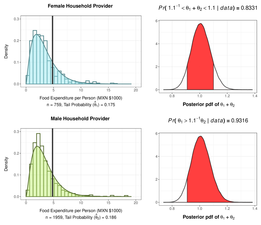
Figure 1: Group-specific summaries for quarterly food expenditure per person. Left: Food expenditure distributions. Right: Visualizations of the posterior and CPMs.

For $j=1$ and 2, we consider the tail probabilities $\theta_{j}=Pr(y_{ij}>4.82)$. The threshold of $\kappa=4.82$ is the median quarterly food expenditure per person (in MXN $1000) for upper income households in Aguascalientes after accounting for weighting factors. Thus, we use the ratio $\theta_{1}/\theta_{2}$ to compare the probabilities that lower-middle income households with female and male providers spend at least as much on food per person as the typical upper income household. The observed proportions of households that spend at least $4820 MXN on food per person are $\hat{\theta}_{1}=0.175$ and $\hat{\theta}_{2}=0.186$. We assign uninformative $\text{GAMMA}(2,0.1)$ priors to both the shape $\alpha_{j}$ and rate $\beta_{j}$ parameters of the gamma model for group $j=1,2$. We let $\boldsymbol{\eta}_{j}=(\alpha_{j},\beta_{j})$ for $j=1,2$. We obtain $10^{5}$ posterior draws for $\boldsymbol{\eta}_{1}$ and $\boldsymbol{\eta}_{2}$ using sampling-resampling methods (Rubin, 1987; Smith and Gelfand, 1992). These posterior draws give rise to draws from the posterior of $\theta_{1}/\theta_{2}$. The gamma distributions characterized by the posterior means for $\boldsymbol{\eta}_{1}$ and $\boldsymbol{\eta}_{2}$ are superimposed on the histograms of the food expenditure data in Figure 1.

To demonstrate equivalence testing, we suppose that $\delta_{*}=0.1$. This implies that a 10% increase or decrease in the probability of spending at least as much on food per person as the typical upper income household is not of practical importance. Figure 1 illustrates that the PoA for this value of $\delta_{*}$ is 0.8331. We consider a conviction threshold of $\gamma=0.9$. Because $0.1<0.8331<0.9$, we refrain from concluding whether $\theta_{1}/\theta_{2}\in(1.1^{-1},1.1)$. Figure 1 also displays the PoNI (0.9316). For $\gamma=0.9$, this noninferiority test indicates that households with female providers are, for practical purposes, at least as likely to spend $\geq\$4820$ MXN on food per person as those with male providers.

3 Theoretical Properties of the SSSD

3.1 The Approximate Normality of the SSSD

The SSSD is defined such that when the sample size $n$ is taken as its $100\times p^{\text{th}}$ percentile, the resulting $100\times(1-\alpha)\%$ HDI will have length at most $l$ with probability at least $p$ (for a given $l$ and $\alpha$). This distribution assumes that data are generated from the selected response distributions parameterized by (fixed) user-specified design values. This approach does not account for uncertainty in the user’s guesses for the design values; however, using fixed parameter values is advantageous because it leads to the approximate normality of the SSSD. This approximate normality is useful because it facilitates fast and accurate sample size calculations.

We now provide theoretical justification for the approximate normality of the SSSD, which relies on the Bernstein-von Mises (BvM) theorem (van der Vaart, 1998). Under certain conditions, the BvM theorem establishes the asymptotic equivalence between Bayesian credible sets of credibility level $1-\alpha$ and confidence sets of confidence level $1-\alpha$. We exploit this asymptotic equivalence between Bayesian and frequentist inference in our approach to sample size determination.

We assume that the data generation process for the two groups is characterized by the models $f(y;\boldsymbol{\eta}_{1,0})$ and $f(y;\boldsymbol{\eta}_{2,0})$. Here, $f(\cdot)$ is the probability density or mass function selected for both groups of data, and $\boldsymbol{\eta}_{1,0}$ and $\boldsymbol{\eta}_{2,0}$ are fixed design values for the distributional parameter(s). These distributions are herein referred to as design distributions. The design values $\boldsymbol{\eta}_{j,0}$ are different from the random variables $\boldsymbol{\eta}_{j}$ that parameterize the model for groups $j=1,2$ in Bayesian settings. To ensure that the SSSD is approximately normal, we require that the models $f(y;\boldsymbol{\eta}_{1,0})$ and $f(y;\boldsymbol{\eta}_{2,0})$ satisfy the regularity conditions for the asymptotic normality of the maximum likelihood estimator (MLE) (Lehmann and Casella, 1998). When specifying the models $f(y;\boldsymbol{\eta}_{j,0})$, we also specify fixed values $\theta_{j,0}$ for the random variables $\theta_{j}$, $j=1,2$. These values are often specified implicitly as a function $g(\cdot)$ of the parameters $\boldsymbol{\eta}_{j,0}$: $\theta_{j,0}=g(\boldsymbol{\eta}_{j,0})$. We require that $g(\boldsymbol{\eta}_{j,0})$ is a differentiable with respect to $\boldsymbol{\eta}_{j,0}$ for $j=1,2$.

Theorem 1 provides the necessary conditions for the approximate normality of the SSSD. The conditions to invoke Theorem 1, including those for the BvM theorem (van der Vaart, 1998) and the regularity conditions from Lehmann and Casella (1998), are detailed in Appendix A of the supplement (Hagar and Stevens, 2023). The approximate normality holds when the SSSD is defined for the posterior of a univariate parameter $\theta=h(\theta_{1},\theta_{2})$, where $h(\cdot)$ is a differentiable function with respect to $\theta_{1}$ and $\theta_{2}$. Here, $h(\theta_{1},\theta_{2})=\theta_{1}-\theta_{2}$ and $h(\theta_{1},\theta_{2})=\theta_{1}/\theta_{2}$ are of interest.

Theorem 1.

Let $f(y;\boldsymbol{\eta}_{1,0})$ and $f(y;\boldsymbol{\eta}_{2,0})$ satisfy the regularity conditions from Appendix A. Let the prior for $\theta_{j}$ be continuous in a neighbourhood of $\theta_{j,0}=g(\boldsymbol{\eta}_{j,0})$ with positive density at $\theta_{j,0}$ for $j=1,2$. For fixed coverage $1-\alpha$, let $L_{1-\alpha}(\boldsymbol{Y}^{{}_{(n)}})$ be the length of the $100\times(1-\alpha)\%$ posterior HDI for $\theta=h(\theta_{1},\theta_{2})$ given to-be-observed data $\boldsymbol{Y}^{{}_{(n)}}$ generated from $f(y;\boldsymbol{\eta}_{1,0})$ and $f(y;\boldsymbol{\eta}_{2,0})$. Let $F_{l}(n)$ be the SSSD’s CDF for $L_{1-\alpha}(\boldsymbol{Y}^{{}_{(n)}})$ with the target interval length $l$. Let $z_{1-\alpha/2}$ be the upper $\alpha/2$-quantile of $\mathcal{N}(0,1)$ and $\mathcal{I}(\theta_{0})$ be the Fisher information for $\theta$ evaluated at $\theta_{0}$. Then,

1. $\sqrt{n}\left(\sqrt{n}L_{1-\alpha}(\boldsymbol{Y}^{{}_{(n)}})-2z_{1-\alpha/2}\mathcal{I}(\theta_{0})^{-\nicefrac{{1}}{{2}}}\right)\xrightarrow{d}\mathcal{N}\left(0,4z^{2}_{1-\alpha/2}A^{2}\right),$ where $A^{2}$ is the asymptotic variance of ${\sqrt{n}}(\mathcal{I}(\hat{\theta}_{n})^{-\nicefrac{{1}}{{2}}}-\mathcal{I}(\theta_{0})^{-\nicefrac{{1}}{{2}}})$.

2. Let $\mu_{l}=4z^{2}_{1-\alpha/2}\mathcal{I}(\theta_{0})^{-1}/l^{2}$, and let $W\in\{0,1\}$ denote whether the length criterion is satisfied. For large sample sizes $n$, $Pr(W=1|N=n)$ is approximately characterized by a univariate probit model with intercept $\beta_{0}=-z_{1-\alpha/2}\mathcal{I}(\theta_{0})^{-\nicefrac{{1}}{{2}}}/\mu_{l}^{\nicefrac{{1}}{{2}}}$, slope $\beta_{1}=z_{1-\alpha/2}\mathcal{I}(\theta_{0})^{-\nicefrac{{1}}{{2}}}/\mu_{l}^{\nicefrac{{3}}{{2}}}$, and error term variance $\sigma^{2}_{\varepsilon}=4z^{2}_{1-\alpha/2}A^{2}/\mu_{l}^{2}$.

3. Let $\sigma_{l}=4z_{1-\alpha/2}A/l$. As $l\rightarrow 0^{+}$, $\dfrac{F_{l}(n)-\mu_{l}}{\sigma_{l}}\xrightarrow{d}\mathcal{N}(0,1).$

Before proving Theorem 1 in Section 3.2, we briefly comment on the conditions required for the SSSD’s approximate normality to hold as $l\rightarrow 0^{+}$. van der Vaart (1998) details four assumptions that must be satisfied in order to invoke the BvM theorem. The first three assumptions involve the models $f(y;\boldsymbol{\eta}_{1,0})$ and $f(y;\boldsymbol{\eta}_{2,0})$ and are weaker than the sufficient regularity conditions for the asymptotic normality of the MLE (Lehmann and Casella, 1998). Therefore, the first three assumptions for the BvM theorem are also necessarily satisfied in Theorem 1. The final assumption regards prior specification for the random variables (van der Vaart, 1998). For our purposes, $\theta_{1}$ and $\theta_{2}$ are the random variables for which we explicitly or implicitly assign prior distributions. We require that the prior distribution of $\theta_{j}$ be continuous in a neighbourhood of $\theta_{j,0}=g(\boldsymbol{\eta}_{j,0})$ with positive density at $\theta_{j,0}$ for $j=1,2$. This condition is important because it ensures that the posterior of $\theta=h(\theta_{1},\theta_{2})$ converges to a neighbourhood of $\theta_{0}=h(\theta_{1,0},\theta_{2,0})$. This convergence ensures the SSSD is well defined in the limiting case. In Appendix B of the supplement, we establish a system for SSSD classification that excludes degenerate and ill-defined SSSDs for the purposes of sample size determination.

3.2 Proof of Theorem 1

We now prove Theorem 1, starting with part $(a)$. Under the conditions for Theorem 1, the BvM theorem states that the posterior of $\theta$ converges to the $\mathcal{N}(\theta_{0},\mathcal{I}(\theta_{0})^{-1}/n)$ distribution in the limit of infinite data (van der Vaart, 1998). The length of the $100\times(1-\alpha)\%$ HDI is defined by this asymptotic variance: $\mathcal{I}(\theta_{0})^{-1}/n$. In practice, $\theta_{0}$ is estimated from the to-be-observed data $\boldsymbol{Y}^{{}_{(n)}}$ using the MLE $\hat{\theta}_{n}$. Given $\alpha$ and large $n$,

$$L_{1-\alpha}(\boldsymbol{Y}^{{}_{(n)}})\approx\dfrac{2z_{1-\alpha/2}}{\sqrt{n}}\times{\mathcal{I}(\hat{\theta}_{n})^{-\nicefrac{{1}}{{2}}}}.$$ (4)

When the conditions for Theorem 1 hold, the delta method ensures that

$$\sqrt{n}\left(2z_{1-\alpha/2}\mathcal{I}(\hat{\theta}_{n})^{-\nicefrac{{1}}{{2}}}-2z_{1-\alpha/2}\mathcal{I}(\theta_{0})^{-\nicefrac{{1}}{{2}}}\right)\xrightarrow{d}\mathcal{N}\left(0,4z^{2}_{1-\alpha/2}A^{2}\right).$$ (5)

The asymptotic variance of ${\sqrt{n}}(\mathcal{I}(\hat{\theta}_{n})^{-\nicefrac{{1}}{{2}}}-\mathcal{I}(\theta_{0})^{-\nicefrac{{1}}{{2}}})$ involves the product of the squared derivative of $\mathcal{I}(\theta)^{-\nicefrac{{1}}{{2}}}$ with respect to $\theta$ evaluated at $\theta_{0}$ and $\mathcal{I}(\theta_{0})^{-1}$. We refer to this asymptotic variance as $A^{2}$ to simplify notation. Part $(a)$ of Theorem 1 follows directly from (4) and (5). This result implies that that for large sample sizes $n$,

$$L_{1-\alpha}(\boldsymbol{Y}^{{}_{(n)}})~{}\dot{\sim}~{}\mathcal{N}\left(\dfrac{2z_{1-\alpha/2}\mathcal{I}(\theta_{0})^{-\nicefrac{{1}}{{2}}}}{\sqrt{n}},\dfrac{4z^{2}_{1-\alpha/2}A^{2}}{n^{2}}\right).$$ (6)

We next prove part $(b)$ of Theorem 1. We first define $\mu_{l}$ as the sample size $n$ such that the approximate normal distribution from (6) has mean of $l$. Equating the mean of this approximate distribution to $l$ and solving for $n$ yields

$$\mu_{l}=\dfrac{4z^{2}_{1-\alpha/2}\mathcal{I}(\theta_{0})^{-1}}{l^{2}}.$$ (7)

We note that $\mu_{l}\rightarrow\infty$ as $l\rightarrow 0^{+}$. We define a variable $W\in\{0,1\}$ that denotes whether the length criterion is satisfied. That is, $W=1$ if and only if $l-L_{1-\alpha}(\boldsymbol{Y}^{{}_{(n)}})\geq 0$. By (6), $l-L_{1-\alpha}(\boldsymbol{Y}^{{}_{(n)}})$ is approximately normal for a given large sample size $n$. We let $N$ be a random variable for the sample size. We now show that conditional on the sample size, the probit model given by

$$\Phi^{-1}(Pr(W=1|N=n))=\dfrac{-z_{1-\alpha/2}\mathcal{I}(\theta_{0})^{-\nicefrac{{1}}{{2}}}}{\mu_{l}^{\nicefrac{{1}}{{2}}}}+\dfrac{z_{1-\alpha/2}\mathcal{I}(\theta_{0})^{-\nicefrac{{1}}{{2}}}}{\mu_{l}^{\nicefrac{{3}}{{2}}}}n,$$ (8)

where the model’s error terms have homoscedastic variance $\sigma_{\varepsilon}^{2}=4z^{2}_{1-\alpha/2}A^{2}/\mu_{l}^{2}$ approximately characterizes $Pr(W=1|N=n)$ for large sample sizes $n$.

The intercept $\beta_{0}$ and slope $\beta_{1}$ of the probit model in (8) define the first-order Taylor approximation to $l-\mathbb{E}(L_{1-\alpha}(\boldsymbol{Y}^{{}_{(n)}}))$ at $n=\mu_{l}$. For large sample sizes $n$ in a neighbourhood of $\mu_{l}$, $\beta_{0}+\beta_{1}n\approx l-\mathbb{E}(L_{1-\alpha}(\boldsymbol{Y}^{{}_{(n)}}))$. It follows from (6) that the approximately normally distributed error terms for $l-L_{1-\alpha}(\boldsymbol{Y}^{{}_{(n)}})$ exhibit heteroscedasticity: $Var(L_{1-\alpha}(\boldsymbol{Y}^{{}_{(n)}}))\approx 4z_{1-\alpha/2}^{2}A^{2}/n^{2}$ decreases as $n$ increases. We demonstrate shortly that the impact of this heteroscedasticity is negligible for large $n$, and we can treat the error terms as having homoscedastic variance $\sigma_{\varepsilon}^{2}$. This result allows us to later prove part $(c)$ of Theorem 1.

If the probit model from (8) is appropriate, then $N$ is normally distributed with mean $-\beta_{0}/\beta_{1}$ and standard deviation $\sigma_{\varepsilon}/\beta_{1}$. It follows by (8) that $-\beta_{0}/\beta_{1}=\mu_{l}$. The standard deviation, which we denote $\sigma_{l,\mu_{l}}$, is given by

$$\dfrac{\sigma_{\varepsilon}}{\beta_{1}}=\dfrac{2z_{1-\alpha/2}A/\mu_{l}}{z_{1-\alpha/2}\mathcal{I}(\hat{\theta}_{n})^{-\nicefrac{{1}}{{2}}}/\mu_{l}^{\nicefrac{{3}}{{2}}}}=4z_{1-\alpha/2}A/l,$$ (9)

where the last equality is obtained by substituting the expression for $\mu_{l}$ from (7).

The value for $l\sigma_{l,\mu_{l}}=4z_{1-\alpha/2}A$ was obtained using $\sigma^{2}_{\varepsilon}=Var(L_{1-\alpha}(\boldsymbol{Y}^{{}_{(\mu_{l})}}))$. For given $l$, we obtain a different value for this quantity using the approximate distribution of $L_{1-\alpha}(\boldsymbol{Y}^{{}_{(n)}})$ for $n\neq\mu_{l}$. We call this quantity $l\sigma_{l,n}$ and consider $n=\mu_{l}+a$ for $\lvert a\rvert<3\sigma_{l,\mu_{l}}$. To show that the impact of heteroscedasticity is negligible for large sample sizes $n$, we consider the limiting behaviour of $l\sigma_{l,n}$. Let $\Phi(\cdot)$ and $\Phi(\cdot;\mu,\sigma)$ respectively be the CDFs of $\mathcal{N}(0,1)$ and $\mathcal{N}(\mu,\sigma^{2})$. By (6), we have that $Pr(L_{1-\alpha}(\boldsymbol{Y}^{{}_{(\mu_{l})}})\leq l)\approx 0.5$ and $Pr(L_{1-\alpha}(\boldsymbol{Y}^{{}_{(n)}})\leq l)\approx\Phi\left(l;2z_{1-\alpha/2}\mathcal{I}(\theta_{0})^{-\nicefrac{{1}}{{2}}}/n^{\nicefrac{{1}}{{2}}},2z_{1-\alpha/2}A/n\right)$. This yields

$$l\sigma_{l,n} =l\times\dfrac{n-\mu_{l}}{\Phi^{-1}\left(Pr(L_{1-\alpha}(\boldsymbol{Y}^{{}_{(n)}})\leq l)\right)-\Phi^{-1}\left(Pr(L_{1-\alpha}(\boldsymbol{Y}^{{}_{(\mu_{l})}})\leq l)\right)}$$

$$=l\times 2z_{1-\alpha/2}A\times\dfrac{1-\mu_{l}/n}{l-2z_{1-\alpha/2}\mathcal{I}(\theta_{0})^{-\nicefrac{{1}}{{2}}}/n^{\nicefrac{{1}}{{2}}}}.$$ (10)

Solving (7) for $l$ and substituting this expression into (10) for $n=\mu_{l}+a$ gives

$$l\sigma_{l,\mu_{l}+a}=2z_{1-\alpha/2}A\times\dfrac{1-\dfrac{1}{1+a/\mu_{l}}}{1-\dfrac{1}{\sqrt{1+a/\mu_{l}}}}.$$ (11)

By L’Hôpital’s rule, the limit of the quotient in (11) is 2 as $\mu_{l}\rightarrow\infty$. It follows that for arbitrary fixed $a$, $\lim_{\mu_{l}\rightarrow\infty}l\sigma_{l,\mu_{l}+a}$ $=4z_{1-\alpha/2}A=l\sigma_{l,\mu_{l}}$. For large sample sizes $n=\mu_{l}+a$, $l\sigma_{l,n}$ does not change drastically, so the impact of heteroscedasticity is not substantial. Therefore, part $(b)$ of Theorem 1 holds true: the probit model from (8) approximately characterizes $Pr(W=1|N=n)$ for large sample sizes $n$.

Lastly, we prove part $(c)$ of Theorem 1. We let $\sigma_{l}=\sigma_{l,\mu_{l}}=4z_{1-\alpha/2}A/l$. We define the probable domain of the SSSD as $\{n~{}|~{}n\in(\mu_{l}~{}\pm~{}3\sigma_{l})\}$. As $l\rightarrow 0^{+}$, both the lower and upper extremes of the SSSD’s probable domain approach $\infty$ because $\mu_{l}$ and $\sigma_{l}$ are functions of $l^{-2}$ and $l^{-1}$, respectively. Because the probit model from part $(b)$ of Theorem 1 is appropriate for large sample sizes $n$ that correspond to small target HDI target lengths $l$, it follows by (9) that the SSSD is approximately normal with mean $\mu_{l}$ and standard deviation $\sigma_{l}$. As $l\rightarrow 0^{+}$, $\sigma_{l}^{-1}(F_{l}(n)-\mu_{l})\xrightarrow{d}\mathcal{N}(0,1).$

3.3 Practical Limitations of Theorem 1

We emphasize that $\mu_{l}=4z^{2}_{1-\alpha/2}\mathcal{I}(\theta_{0})^{-1}/l^{2}$ and $\sigma_{l}=4z_{1-\alpha/2}A/l$ defined in Theorem 1 do not incorporate information from the relevant prior distributions; they depend solely on the design distributions $f(y;\boldsymbol{\eta}_{1,0})$ and $f(y;\boldsymbol{\eta}_{2,0})$ and the choices for $l$ and $\alpha$. The design distributions impact $\mu_{l}$ and $\sigma_{l}$ via $\mathcal{I}(\theta_{0})^{-1}$ and $A$, respectively. For large sample sizes $n$ corresponding to small target lengths $l$, these values for $\mu_{l}$ and $\sigma_{l}$ can be used to determine percentiles of the SSSD. We formally state this result in Corollary 1, which follows from Theorem 1.

Corollary 1.

Let $\mu_{l}=4z^{2}_{1-\alpha/2}\mathcal{I}(\theta_{0})^{-1}/l^{2}$ and $\sigma_{l}=4z_{1-\alpha/2}A/l$. If we obtain a sample of size $n=\mu_{l}+z_{p}\sigma_{l}$ from both $f(y;\boldsymbol{\eta}_{1,0})$ and $f(y;\boldsymbol{\eta}_{2,0})$, the probability that the $100\times(1-\alpha)\%$ posterior HDI for $\theta$ satisfies the length criterion approaches $p$ as $l\rightarrow 0^{+}$.

These values for $\mu_{l}$ and $\sigma_{l}$ technically ensure that the $100\times(1-\alpha)\%$ confidence interval for $\theta$ has length at most $l$ with probability at least $p$ for fixed $\alpha$. But because the BvM theorem establishes the asymptotic equivalence between $100\times{(1-\alpha)}\%$ credible and confidence intervals, we are ensured that the $100\times(1-\alpha)\%$ HDI for the posterior of $\theta$ also has length at most $l$ with probability at least $p$ for reasonably large sample sizes. Similarly to how asymptotic normality is exploited for finite samples, we do not require that $l=0$ to invoke Theorem 1. However, it is not trivial to determine how small $l$ must be to yield a sample size $n$ that is large enough to blunt the impact of prior information on the posterior of $\theta$. Corollary 1 is therefore only useful in the limiting case with large sample sizes. Nevertheless, the theoretical results from this section are valuable. In Section 5, we leverage insights from Theorem 1 to develop a method that prompts better sample size recommendations in moderate sample size scenarios.

4 Stage 1: Aligning Interval-Based Criteria and Power

4.1 Choosing Targets for the HDI Length and Coverage

To use the SSSD for sample size determination, we must specify a target length $l$ and coverage $1-\alpha$ for the posterior HDI of $\theta$. Because we aim to draw a conclusion about whether $\theta\in(\delta_{1},\delta_{2})$ using a conviction threshold $\gamma$, we suggest selecting interval-based criteria that align with a target power $\Gamma$ defined in (3). We aim for $100\times\gamma\%$ of the posterior of $\theta$ to be contained in $(\delta_{1},\delta_{2})$. As such, it would be natural to work with $100\times\gamma\%$ HDIs, and we recommend choosing $\alpha=1-\gamma$. It follows that the target length $l$ should be less than $\delta_{2}-\delta_{1}$: if we do not expect $100\times(1-\alpha)\%$ of the posterior to fall in any interval of length $\delta_{2}-\delta_{1}$, then we cannot expect $100\times\gamma\%$ of the posterior to be contained within the interval $(\delta_{1},\delta_{2})$. However, it is not clear how much smaller $l$ should be than $\delta_{2}-\delta_{1}$. If $\theta_{0}$ is close to $\delta_{1}$ or $\delta_{2}$, then $l$ should likely be substantially smaller. Lastly, we note that the SSSD can also be used when $l$ and $\alpha$ are not selected to align with power-based criteria.

In this section, we describe the first of two stages in our procedure for sample size determination. This first stage does not account for the prior distributions; it implicitly selects a target length $l$ for the SSSD based on a target power $\Gamma$, along with the design distributions and interval $(\delta_{1},\delta_{2})$. It should be more intuitive for practitioners to choose $\Gamma$ than guess a value for $l<\delta_{2}-\delta_{1}$. Aligning $l$ with $\Gamma$ requires some knowledge of the power curve, which can be computationally intensive to estimate.

4.2 Fast Approximation of the Power Curve

Traditional approaches to power curve estimation are slow for several reasons. First, we must simulate many samples from the design distributions to reliably estimate power for each value of $n$ explored. Second, in the absence of conjugate priors, we must use computational methods to approximate the posterior corresponding to each generated sample. Third, we must choose which sample sizes $n$ to explore, and we may waste time considering sample sizes that are much too large or small.

Because we aim to roughly estimate the power curve to select an appropriate HDI target length $l$, we develop an approach for power curve approximation that addresses these sources of computational inefficiency. For a given sample $\boldsymbol{y}^{{}_{(n)}}$, we can compute maximum likelihood estimates $\hat{\boldsymbol{\eta}}_{1,n}$ and $\hat{\boldsymbol{\eta}}_{2,n}$, which yield an estimate for $\hat{\theta}_{n}$ via the functions $g(\cdot)$ and $h(\cdot)$. For sufficiently large $n$, the posterior of $\theta$ is approximately $\mathcal{N}(\hat{\theta}_{n},\mathcal{I}(\hat{\theta}_{n})^{-1}/n)$. We can quickly determine whether $100\times\gamma\%$ of the $\mathcal{N}(\hat{\theta}_{n},\mathcal{I}(\hat{\theta}_{n})^{-1}/n)$ distribution is contained within the interval $(\delta_{1},\delta_{2})$. Given a representative sample of $\hat{\theta}_{n}$ values corresponding to samples from $f(y;\boldsymbol{\eta}_{1,0})$ and $f(y;\boldsymbol{\eta}_{2,0})$, the proportion of time that this occurs would roughly estimate power at the sample size $n$.

Given a sample size $n$, we do not simulate data $\boldsymbol{Y}^{{}_{(n)}}$ from the prior predictive distribution. We instead simulate from the approximate distributions of the MLEs of ${\boldsymbol{\eta}}_{1}$ and ${\boldsymbol{\eta}}_{2}$. For sufficiently large $n$, the MLEs $\hat{\boldsymbol{\eta}}_{j,n}$ for groups $j=1,2$ approximately and independently follow $\mathcal{N}(\boldsymbol{\eta}_{j,0},I^{-1}(\boldsymbol{\eta}_{j,0})/n)$ distributions. We use low-discrepancy sequences and conditional probability distributions to obtain a sample of moderate size from the joint limiting distribution of $\hat{\boldsymbol{\eta}}_{1,n}$ and $\hat{\boldsymbol{\eta}}_{2,n}$. Both $\hat{\boldsymbol{\eta}}_{1,n}$ and $\hat{\boldsymbol{\eta}}_{2,n}$ have dimension $d$, so their joint limiting distribution has dimension $2d$. We use a Sobol’ sequence $\boldsymbol{u}_{1},\boldsymbol{u}_{2},...,\boldsymbol{u}_{n_{sob}}\in[0,1]^{2d}$ (Sobol’, 1967) with length $n_{sob}$. Sobol’ sequences are low-discrepancy sequences based on integer expansion in base 2. Randomized Sobol’ sequences yield estimators with better consistency properties than those created using deterministic sequences, and this randomization can be carried out via a digital shift (Lemieux, 2009). We generate and randomize Sobol’ sequences in R using the qrng package (Hofert and Lemieux, 2020). The dimension of the data $\boldsymbol{Y}^{{}_{(n)}}$ is typically such that $d<<n$. It is therefore easier to obtain an efficient and representative sample from the joint distribution of $\hat{\boldsymbol{\eta}}_{1,n}$ and $\hat{\boldsymbol{\eta}}_{2,n}$ using low-discrepancy sampling methods.

In practice, we may require fewer observations for these limiting distributions to be approximately normal if we consider some transformation of ${\boldsymbol{\eta}}_{j}$. For the gamma model, both parameters in ${\boldsymbol{\eta}}_{j}=(\alpha_{j},\beta_{j})$ must be positive, but the $\mathcal{N}(\boldsymbol{\eta}_{j,0},I^{-1}(\boldsymbol{\eta}_{j,0})/n)$ distribution could admit nonpositive values for small $n$. To obtain a sample of positive $\hat{\boldsymbol{\eta}}_{1,n}$ and $\hat{\boldsymbol{\eta}}_{2,n}$ values for any sample size $n$ with the gamma model, we exponentiate a sample of approximately normal MLEs of $\text{log}({\boldsymbol{\eta}}_{1})$ and $\text{log}({\boldsymbol{\eta}}_{2})$. These approximately normal distributions can be found using the multivariate delta method. For an arbitrary model, appropriate transformations could similarly be applied to any parameters in ${\boldsymbol{\eta}}_{j}$ that do not have support on $\mathbb{R}$.

Each draw $(\hat{\boldsymbol{\eta}}_{1,n}(\boldsymbol{u}_{r}),\hat{\boldsymbol{\eta}}_{2,n}(\boldsymbol{u}_{r}))$ from the joint limiting distribution depends solely on the design distributions and the Sobol’ sequence draw $\boldsymbol{u}_{r},~{}r=1,...,n_{sob}$. We recommend using $n_{sob}=1024$. We use the notation $(\hat{\boldsymbol{\eta}}_{1,n}(\boldsymbol{u}_{r}),\hat{\boldsymbol{\eta}}_{2,n}(\boldsymbol{u}_{r}))$ but emphasize that $\hat{\boldsymbol{\eta}}_{1,n}(\boldsymbol{u}_{r})$ and $\hat{\boldsymbol{\eta}}_{2,n}(\boldsymbol{u}_{r})$ are functions of only the first and final $d$ components of $\boldsymbol{u}_{r}\in[0,1]^{2d}$, respectively. For each draw $(\hat{\boldsymbol{\eta}}_{1,n}(\boldsymbol{u}_{r}),\hat{\boldsymbol{\eta}}_{2,n}(\boldsymbol{u}_{r}))$, we consider the distributions $f(y;\hat{\boldsymbol{\eta}}_{1,n}(\boldsymbol{u}_{r}))$ and $f(y;\hat{\boldsymbol{\eta}}_{2,n}(\boldsymbol{u}_{r}))$. Upon computing these draws for a given value of $n$, we treat $\boldsymbol{\eta}_{1,r}=\hat{\boldsymbol{\eta}}_{1,n}(\boldsymbol{u}_{r})$ and $\boldsymbol{\eta}_{2,r}=\hat{\boldsymbol{\eta}}_{2,n}(\boldsymbol{u}_{r})$ as fixed design values for $r=1,...,n_{sob}$. This allows us to compute $\theta_{j,r}=g(\boldsymbol{\eta}_{1,r})$ for $j=1,2$, yielding $\theta_{r}=h(\theta_{1,r},\theta_{2,r})$ and $\mathcal{I}(\theta_{r})^{-1}$. To find $\mathcal{I}(\theta_{0})^{-1}$, we find the limiting distributions for $\sqrt{n}(\hat{\boldsymbol{\eta}}_{j,n}-\boldsymbol{\eta}_{j,0})$, $j=1,2$. The multivariate delta method prompts the limiting distribution for $\sqrt{n}(\hat{\theta}_{n}-\theta_{0})$, where $\hat{\theta}_{n}$ is a function of $\hat{\boldsymbol{\eta}}_{1,n}$ and $\hat{\boldsymbol{\eta}}_{2,n}$. The variance of this limiting distribution is $\mathcal{I}(\theta_{0})^{-1}$. To find $\mathcal{I}(\theta_{r})^{-1}$, we replace the fixed values $\theta_{0},\boldsymbol{\eta}_{1,0}$, and $\boldsymbol{\eta}_{2,0}$ with their counterparts determined by $\boldsymbol{\eta}_{1,r}$ and $\boldsymbol{\eta}_{2,r}$.

For $r=1,...,n_{sob}$, we consider the limiting posterior imposed by the BvM theorem: $\mathcal{N}(\theta_{r},\mathcal{I}(\theta_{r})^{-1}/n)$. For ratio-based comparisons with moderate sample sizes, the posterior of $\text{log}(\theta_{1})-\text{log}(\theta_{2})$ may be better approximated by a normal distribution than that of $\theta_{1}/\theta_{2}$. Given that posterior probabilities are invariant to monotonic transformations, we suggest considering the posterior of $\theta=\text{log}(\theta_{1})-\text{log}(\theta_{2})$ in those scenarios. We then determine whether $100\times\gamma\%$ of the limiting posterior is contained within the interval $(\delta_{1},\delta_{2})$ for $r=1,...,n_{sob}$. The proportion of the $n_{sob}$ times that this occurs roughly estimates the value of the power curve at $n$. If we repeat this process for several appropriate values of $n$, we can roughly approximate the entire power curve. Unfortunately, such a process would still require users to choose appropriate sample sizes $n$, limiting its efficiency and usability. We now argue that the user does not need to choose the values of $n$ if we appeal to the convexity of the $(\theta_{1},\theta_{2})$-space such that $\theta=h(\theta_{1},\theta_{2})\in(\delta_{1},\delta_{2})$ when $\theta=\theta_{1}-\theta_{2}$ or $\theta=\theta_{1}/\theta_{2}$. We illustrate that these regions are indeed convex in Appendix C.1 of the supplement.

We note that $(\theta_{1,r},\theta_{2,r})$ depends on $n$ through the sample size of the joint limiting distribution for $\hat{\boldsymbol{\eta}}_{1,n}$ and $\hat{\boldsymbol{\eta}}_{2,n}$. We now fix the draw $\boldsymbol{u}_{r}$ and let the sample size $n$ vary; to make this more clear, we let $\theta_{j,r}=\theta_{j,r}^{{}_{(n)}}$. For a given draw $\boldsymbol{u}_{r}$, $(\hat{\boldsymbol{\eta}}_{1,n}(\boldsymbol{u}_{r}),\hat{\boldsymbol{\eta}}_{2,n}(\boldsymbol{u}_{r}))$ will be closer to $(\boldsymbol{\eta}_{1,0},\boldsymbol{\eta}_{2,0})$ for larger values of $n$ by properties of conditional multivariate normal distributions. Although not guaranteed, $(\theta_{1,r}^{{}_{(n)}},\theta_{2,r}^{{}_{(n)}})$ should also generally be closer to $(\theta_{1,0},\theta_{2,0})$ for larger values of $n$. It follows that for larger values of $n$, (i) the mean of the $\mathcal{N}(\theta_{r}^{{}_{(n)}},\mathcal{I}(\theta_{r}^{{}_{(n)}})^{-1}/n)$ distribution should generally be closer to $\theta_{0}$ and (ii) this distribution should generally have smaller variance. We now consider what is likely to occur when $\theta_{0}\in(\delta_{1},\delta_{2})$ and for a given draw $\boldsymbol{u}_{r}$. If $100\times\gamma\%$ of the $\mathcal{N}(\theta_{r}^{{}_{(n_{A})}},\mathcal{I}(\theta_{r}^{{}_{(n_{A})}})^{-1}/n_{A})$ distribution is contained in the interval $(\delta_{1},\delta_{2})$, then $100\times\gamma\%$ of the $\mathcal{N}(\theta_{r}^{{}_{(n_{B})}},\mathcal{I}(\theta_{r}^{{}_{(n_{B})}})^{-1}/n_{B})$ distribution should also generally be contained in $(\delta_{1},\delta_{2})$ for $n_{A}<n_{B}$. In light of this, our method to roughly approximate the power curve generates a single Sobol’ sequence of length $n_{sob}$. We use root finding algorithms (Brent, 1973) to find the smallest sample size $n$ such that $100\times\gamma\%$ of the $\mathcal{N}(\theta_{r}^{{}_{(n)}},\mathcal{I}(\theta_{r}^{{}_{(n)}})^{-1}/n)$ distribution is contained in the interval $(\delta_{1},\delta_{2})$ for $r=1,...,n_{sob}$. We use the empirical CDF of these $n_{sob}$ sample sizes to approximate the power curve.

This approach requires several simplifying assumptions, though only one is not already required by Theorem 1: the convexity of the region such that $\theta\in(\delta_{1},\delta_{2})$. In situations where the BvM theorem can be leveraged, the usability and computational efficiency of this approach to power curve approximation justify its reliance on simplifying assumptions. If we generated samples of various sizes $n$ from $f(y;\boldsymbol{\eta}_{1,0})$ and $f(y;\boldsymbol{\eta}_{2,0})$ to approximate the power curve, we would need to collectively generate substantially more than $n_{sob}$ samples. In Section 6.2, we show that this approach yields adequate power curve approximation when the BvM theorem can be reasonably applied.

4.3 An Approach to Estimate the SSSD Using Theorem 1

Algorithm 1 formally describes how to implement the first stage of our sample size determination procedure. This stage calibrates the target length $l$ for the SSSD with power-based criteria and estimates this SSSD using Theorem 1. To implement this stage, we must choose a parametric statistical model for both groups, characteristics $\theta_{1}$ and $\theta_{2}$, an interval $(\delta_{1},\delta_{2})$, a conviction threshold $\gamma$, a target power $\Gamma$, and design values ${\boldsymbol{\eta}}_{1,0}$ and ${\boldsymbol{\eta}}_{2,0}$. In general, we recommend using visualization techniques to help choose the design values. The literature on prior elicitation could be of use when specifying the design distributions (Chaloner, 1996; Garthwaite et al., 2005; Johnson et al., 2010). We also discuss how to modify the SSSD estimation procedure when users wish to choose values for $l$ and $\alpha$ that are not calibrated with power-based criteria.

Algorithm 1 Procedure to Estimate the SSSD with Power-Calibrated Target Length

1:procedure StageOne($\gamma,\Gamma$, $\theta_{1}$, $\theta_{2}$, $\delta_{1}$, $\delta_{2}$, $n_{sob}$, $f(y;\boldsymbol{\eta}_{1,0})$, $f(y;\boldsymbol{\eta}_{2,0})$)

2:     sampSobol $\leftarrow\textsc{null}$

3:     for $r$ in [1, $n_{sob}$] do

4:         Generate Sobol’ sequence draw $\boldsymbol{u}_{r}$

5:         Let $\texttt{sampSobol}[r]$ be the smallest sample size $n$ such that $100\times\gamma\%$ of the           $\mathcal{N}(\theta_{r}^{{}_{(n)}},\mathcal{I}(\theta_{r}^{{}_{(n)}})^{-1}/n)$ distribution is contained in the interval $(\delta_{1},\delta_{2})$      

6:     Let $\mu_{l}$ be the $\Gamma$-quantile of sampSobol

7:     Let $\alpha=1-\gamma$

8:     Use the multivariate delta method to find $\mathcal{I}(\theta_{0})^{-1}$

9:     Let $l=2z_{1-\alpha/2}\mathcal{I}(\theta_{0})^{-1/2}/\sqrt{\mu_{l}}$

10:     Let $A^{2}$ be the variance of the limiting distribution for ${\sqrt{n}}(\mathcal{I}(\hat{\theta}_{n})^{-1/2}-\mathcal{I}(\theta_{0})^{-1/2})$

11:     Let $\sigma_{l}=4z_{1-\alpha/2}A/l$

12:     return $\mu_{l}$, $\sigma_{l}$, $l$, $\alpha$, and sampSobol

Lines 2 to 5 of Algorithm 1 summarize the process to roughly approximate the power curve developed in Section 4.2. This subprocess returns a vector of sample sizes sampSobol. Line 6 shows that we calibrate the length criterion with the target power $\Gamma$ by choosing $\mu_{l}$ to be the $\Gamma$-quantile of sampSobol. In Line 7, we choose the coverage $1-\alpha$ of the posterior HDI to coincide with the conviction threshold $\gamma$. Line 8 notes that we must compute $\mathcal{I}(\theta_{0})^{-1}$ as detailed in Section 4.2. Line 9 rearranges the formula in (7) to select a target length $l$ that yields the desired value of $\mu_{l}$ for fixed HDI coverage $1-\alpha$. This calibrates the length criterion and power criterion when $\boldsymbol{Y}^{{}_{(n)}}\sim p(\boldsymbol{y}^{{}_{(n)}})$. The median of the SSSD is a sample size $n$ such that (i) the posterior HDI for $\theta$ has expected length of $l$ and (ii) we expect that $CPM\geq\gamma$ with probability $\Gamma$.

If one wants to use alternative values for $l$ and $\alpha$, they could skip Lines 2 to 7 of Algorithm 1. In Line 9, they would return $\mu_{l}=4z^{2}_{1-\alpha/2}\mathcal{I}(\theta_{0})^{-1}/l^{2}$ as in (7). This is the only modification in this case. To estimate $\sigma_{l}$ as described in Section 3.2, we must first find $A^{2}$, the variance of the limiting distribution for ${\sqrt{n}}(\mathcal{I}(\hat{\theta}_{n})^{-1/2}-\mathcal{I}(\theta_{0})^{-1/2})$ as outlined in Line 10. The multivariate delta method can again be used to find this approximately normal distribution: ${\sqrt{n}}(\mathcal{I}(\hat{\theta}_{n})^{-1/2}-\mathcal{I}(\theta_{0})^{-1/2})$ is also a function of $\hat{\boldsymbol{\eta}}_{1,n}$ and $\hat{\boldsymbol{\eta}}_{2,n}$. To implement the multivariate delta method, numerical methods (Gilbert and Varadhan, 2016) can be used to compute the partial derivatives of $\mathcal{I}(\theta_{0})^{-1/2}$ with respect to ${\boldsymbol{\eta}}_{1,0}$ and ${\boldsymbol{\eta}}_{2,0}$. Given $A^{2}$, we estimate $\sigma_{l}$ as detailed in Line 11. The output returned in Line 12 is used in the second stage of our sample size determination procedure.

5 Stage 2: Accounting for the Prior Distributions

5.1 Motivation

In this section, we introduce the second stage of our sample size determination method. This stage uses simulation to estimate an SSSD that accounts for the prior distributions; it also quickly yields a local approximation to the power curve that incorporates prior information. This approach assumes that the SSSD is approximately normal, which is a reasonable assumption because we still require that the conditions for Theorem 1 are satisfied. The simulation-based method, however, relaxes the requirement that the posterior of $\theta$ is approximately $\mathcal{N}(\theta_{0},\mathcal{I}(\theta_{0})^{-1}/n)$. This is useful when the sample size $n$ is large enough to ensure the posterior of $\theta$ is approximately normal but not large enough to guarantee the relevant priors have no substantial impact on the posterior mean and variance. In Section 5.2, we present a fast method to approximate the expected posterior HDI length for a given sample size $n$. This method to approximate $\mathbb{E}(L_{1-\alpha}(\boldsymbol{Y}^{{}_{(n)}}))$ is incorporated into the SSSD estimation and corresponding power curve approximation procedures we propose in Section 5.3.

5.2 Fast Approximation of Expected HDI Length

To quickly estimate $\mathbb{E}(L_{1-\alpha}(\boldsymbol{Y}^{{}_{(n)}}))$ for a sample size $n$, we generate a non-random, representative sample from $f(y;\boldsymbol{\eta}_{1,0})$ and $f(y;\boldsymbol{\eta}_{2,0})$ as follows. We split the unit interval into $\lceil n\rceil$ equally sized sections: $\{[k-1,k)/\lceil n\rceil\}_{k=1}^{\lceil n\rceil}$. We use the midpoint from each section, $(k-0.5)/\lceil n\rceil$ for $k=1,2,...,\lceil n\rceil$, to generate an observation from each group of design data using CDF inversion on $F(y;\boldsymbol{\eta}_{1,0})$ and $F(y;\boldsymbol{\eta}_{2,0})$. Thus, the empirical CDF of this sample from each group is similar to the CDF of its design distribution.

We do not approximate the posterior for this representative sample using Markov chain Monte Carlo (MCMC) or sampling-resampling methods. For $j=1$ and 2, we instead consider the following multivariate normal approximation that is based on the Taylor series expansion of $\text{log}(p_{j}(\boldsymbol{\eta}_{j}\hskip 1.0pt|\hskip 1.0ptdata))$ centered at the posterior mode $\boldsymbol{\eta}_{j}^{*}=\text{arg\,max}_{{\boldsymbol{\eta}_{j}}}~{}p_{j}(\boldsymbol{\eta}_{j}\hskip 1.0pt|\hskip 1.0ptdata)$ (Gelman et al., 2013):

$$\mathcal{N}\left(\boldsymbol{\eta}_{j}^{*},\left[\dfrac{\partial^{2}}{\partial\boldsymbol{\eta}_{j}^{2}}\text{log}(p(\boldsymbol{\eta}_{j}|\hskip 1.0ptdata))\bigg{\lvert}_{\boldsymbol{\eta}_{j}=\boldsymbol{\eta}_{j}^{*}}\right]^{-1}\right).$$ (12)

Even if numerical methods (Hasselman, 2023) are used to find the posterior modes, this process is faster than approximating the posterior of $\boldsymbol{\eta}_{j}$ using computational methods. For components of $\boldsymbol{\eta}_{j}$ that do not have support over $\mathbb{R}$, we find the normal approximation to the posterior of a transformation of those $\boldsymbol{\eta}_{j}$ parameters. For the gamma distribution, we find a normal approximation to the joint posterior of $\text{log}(\alpha_{j})$ and $\text{log}(\beta_{j})$, $j=1,2$. We do not use the normal approximation from (12) when approximating the power curve in Section 4.2 because that would require us to generate samples of discrete sizes $n$. Consequently, the runtime of the method from Section 4.2 would increase, and the functions passed into the root-finding algorithm would be less smooth.

After obtaining normal approximations to $p_{1}(\boldsymbol{\eta}_{1}\hskip 1.0pt|\hskip 1.0ptdata)$ and $p_{2}(\boldsymbol{\eta}_{2}\hskip 1.0pt|\hskip 1.0ptdata)$, we use the delta method to get an approximately normal posterior for $\theta=h(\theta_{1},\theta_{2})$ that accounts for the prior distributions $p_{1}(\theta_{1})$ and $p_{2}(\theta_{2})$. The length of the $100\times(1-\alpha)\%$ HDI for this distribution, denoted $\bar{L}_{1-\alpha}(\boldsymbol{Y}^{{}_{(n)}})$, serves as a rough estimate for $\mathbb{E}(L_{1-\alpha}(\boldsymbol{Y}^{{}_{(n)}}))$. In most cases, it is not a substantial limitation to assume the posterior of $\theta$ is normal because that is already required for the SSSD’s approximate normality. For ratio-based comparisons with moderate sample sizes, users interested in power-based sample size determination may want define the SSSD for the posterior of $\theta=\text{log}(\theta_{1})-\text{log}(\theta_{2})$. We often require less data for this posterior to be approximately normal compared to that of $\theta_{1}/\theta_{2}$. Since posterior HDIs are not invariant to monotonic transformations, the SSSD should still be defined for the posterior of $\theta_{1}/\theta_{2}$ if this posterior must satisfy the length criterion with desired probability $p$ for interval-based sample size determination.

We comment on why the rough estimate $\bar{L}_{1-\alpha}(\boldsymbol{Y}^{{}_{(n)}})$ is suitable. For a particular analysis prior and sample size $n$, the length of the $100\times(1-\alpha)\%$ HDI depends on $\boldsymbol{Y}^{{}_{(n)}}$, which we assume is generated by the design distributions. The data can be summarized by the MLEs $\hat{\boldsymbol{\eta}}_{1,n}$ and $\hat{\boldsymbol{\eta}}_{2,n}$. For large sample sizes $n$, these MLEs are approximately jointly normally distributed in a neighbourhood of $({\boldsymbol{\eta}}_{1,0},{\boldsymbol{\eta}}_{2,0})$. The size of this neighbourhood around $({\boldsymbol{\eta}}_{1,0},{\boldsymbol{\eta}}_{2,0})$ decreases as $n$ increases. In general, $L_{1-\alpha}(\hat{\boldsymbol{\eta}}_{1,n},\hat{\boldsymbol{\eta}}_{2,n}):\mathbb{R}^{2d}\rightarrow\mathbb{R}^{+}$ is not a linear function, but its linear approximation is often serviceable near $({\boldsymbol{\eta}}_{1,0},{\boldsymbol{\eta}}_{2,0})$. Because of this approximate linearity and the symmetry of the limiting multivariate normal distribution for $(\hat{\boldsymbol{\eta}}_{1,n},\hat{\boldsymbol{\eta}}_{2,n})$, the length of the $100\times(1-\alpha)\%$ HDI at $(\hat{\boldsymbol{\eta}}_{1,n},\hat{\boldsymbol{\eta}}_{2,n})=({\boldsymbol{\eta}}_{1,0},{\boldsymbol{\eta}}_{2,0})$ should provide a rough approximation of $\mathbb{E}(L_{1-\alpha}(\boldsymbol{Y}^{{}_{(n)}}))$.

5.3 An Approach to Adjust for Prior Information

This subsection presents an efficient simulation-based approach to estimate the SSSD. For sample size determination with the gamma example from Section 2, the simulation-based approach proposed here takes roughly 5 seconds on a standard laptop without parallelization; the SSSD estimation method proposed in Stevens and Hagar (2022) takes about 10 hours with substantial parallelization. Our new approach also provides a quick local approximation to the power curve that accounts for the prior distributions.

Algorithm 2 describes the second stage of our sample size determination procedure. Our method for fast sample size determination involves implementing Algorithms 1 and 2 in succession. Algorithm 2 efficiently estimates the SSSD with more flexibility by allowing the components of the probit model ($\beta_{0}$, $\beta_{1}$, and $\sigma_{\varepsilon}$) to vary from their limiting forms dictated by Theorem 1. Generally, this approach involves finding $\tilde{\mu}_{l}$, an estimate for the SSSD mean that incorporates prior information. We then leverage $\tilde{\mu}_{l}$ obtain estimates for the probit model components that account for the prior distributions.

Algorithm 2 Procedure to Adjust for Prior Information with SSSD Estimation

1:procedure StageTwo($\gamma,\Gamma$, $\delta_{1}$, $\delta_{2}$, $n_{var}$, $f(y;\boldsymbol{\eta}_{1,0})$, $f(y;\boldsymbol{\eta}_{2,0})$, $p_{1}(\theta_{1})$, $p_{2}(\theta_{2})$)

2:     Obtain $l$, $\alpha$, sampSobol, and limiting values for $\mu_{l}$ and $\beta_{1}$ via Algorithm 1

3:     Obtain $\tilde{\mu}_{l}$, an estimate for the SSSD mean that incorporates prior information

4:     lenSobol $\leftarrow\textsc{null}$; pwrSobol $\leftarrow\textsc{null}$

5:     for $r$ in [1, $n_{var}$] do

6:         Generate Sobol’ sequence draw $\boldsymbol{u}_{r}$

7:         Generate a non-random sample $\boldsymbol{y}^{{}_{(n)}}$ of size $n=\lceil\tilde{\mu}_{l}\rceil$ from $f(y;\hat{\boldsymbol{\eta}}_{1,n}(\boldsymbol{u}_{r}))$ and            $f(y;\hat{\boldsymbol{\eta}}_{2,n}(\boldsymbol{u}_{r}))$ and approximate the posterior

8:         Let $\texttt{lenSobol}[r]$ be the estimated length of the $100\times(1-\alpha)\%$ posterior HDI

9:         Let $\texttt{pwrSobol}[r]$ be $\mathbb{I}(Pr(\delta_{1}<\theta<\delta_{2}|\hskip 1.0pt\boldsymbol{y}^{{}_{(n)}})\geq\gamma))$      

10:     Let $\hat{\sigma}_{\varepsilon}$ $\leftarrow\texttt{sd(lenSobol)}$

11:     Let $\tilde{\Gamma}$ $\leftarrow\texttt{mean(pwrSobol)}$

12:     Estimate $\mathbb{E}(L_{1-\alpha}(\boldsymbol{Y}^{{}_{(n)}}))$ at several sample sizes near $\tilde{\mu}_{l}$

13:     Fit a linear model to these estimates to obtain $\hat{\beta}_{0}$ and $\hat{\beta}_{1}$

14:     Let $\hat{\mu}_{l}\leftarrow-\hat{\beta}_{0}/\hat{\beta}_{1}$ and $\hat{\sigma}_{l}\leftarrow\hat{\sigma}_{\varepsilon}/\hat{\beta}_{1}$

15:     Use $\tilde{\Gamma}$ to proportionally adjust the power curve for prior information

16:     Let $\tilde{p}$ be the quantile of the SSSD that roughly corresponds to power $\Gamma$

17:     return $\hat{\mu}_{l}$, $\hat{\sigma}_{l}$, $\tilde{p}$, and the approximate power curve $\tilde{F}(n)$

In Line 2 of Algorithm 2, we implement Algorithm 1 to obtain an HDI target length $l$ and coverage $1-\alpha$ along with the limiting values for $\mu_{l}$ and $\beta_{1}$ from Theorem 1. To find an estimate $\tilde{\mu}_{l}$ that incorporates prior information in Line 3, we compute $\bar{L}_{1-\alpha}(\boldsymbol{Y}^{{}_{(\mu_{l})}})$ and let $\dot{\mu}_{l}$ be the horizontal intercept of the line with slope $\beta_{1}$ that traverses the point $(\mu_{l},l-\bar{L}_{1-\alpha}(\boldsymbol{Y}^{{}_{(\mu_{l})}}))$. We then compute $\bar{L}_{1-\alpha}(\boldsymbol{Y}^{{}_{(\dot{\mu}_{l})}})$ and let $\tilde{\mu}_{l}$ be the horizontal intercept of the line passing through $(\mu_{l},l-\bar{L}_{1-\alpha}(\boldsymbol{Y}^{{}_{(\mu_{l})}}))$ and $(\dot{\mu}_{l},l-\bar{L}_{1-\alpha}(\boldsymbol{Y}^{{}_{(\dot{\mu}_{l})}}))$.

Lines 4 to 11 detail a process to efficiently estimate $\sigma_{\varepsilon}$. We obtain this estimate via a modified Monte Carlo integration scheme. As in Section 4.2, we obtain a sample of size $n_{var}$ from the joint limiting distribution of $\hat{\boldsymbol{\eta}}_{1,n}$ and $\hat{\boldsymbol{\eta}}_{2,n}$ for $n=\lceil\tilde{\mu}_{l}\rceil$ using a Sobol’ sequence $\boldsymbol{u}_{1},...,\boldsymbol{u}_{n_{var}}$ and conditional multivariate normal distributions. We use $n_{var}=256$ in our numerical studies. For each Sobol’ sequence draw $\boldsymbol{u}_{r}$, we follow the process in Section 5.2 to generate a non-random sample $\boldsymbol{y}^{{}_{(n)}}$ from $f(y;\hat{\boldsymbol{\eta}}_{1,n}(\boldsymbol{u}_{r}))$ and $f(y;\hat{\boldsymbol{\eta}}_{2,n}(\boldsymbol{u}_{r}))$. For the normal approximation to the posterior of each sample, we compute the $100\times(1-\alpha)\%$ HDI length. The standard deviation of these $n_{var}$ lengths provides a rough estimate for $\sigma_{\varepsilon}$ as illustrated in Line 10. For each approximately normal posterior, we also record whether the estimate for $Pr(\delta_{1}<\theta<\delta_{2}|\hskip 1.0pt\boldsymbol{y}^{{}_{(n)}})$ is greater than the conviction threshold $\gamma$. This yields a quick, rough estimate for the power of the equivalence test at $n=\lceil\tilde{\mu}_{l}\rceil$ in Line 11, which will be used later.

The last component of the probit model we estimate is the linear approximation to $l-\mathbb{E}(L_{1-\alpha}(\boldsymbol{Y}^{{}_{(n)}}))$ near the SSSD’s mean. Line 12 of Algorithm 2 mentions this process, in which we compute $\bar{L}_{1-\alpha}(\boldsymbol{Y}^{{}_{(n)}})$ for several values near the SSSD mean. We obtain penultimate estimates for $\mu_{l}$ and $\sigma_{l}$ to know which sample sizes $n$ to consider. We get these estimates, $\ddot{\mu}_{l}$ and $\ddot{\sigma}_{l}$, by using the estimate for $\sigma_{\varepsilon}$ and the line passing through the points $(\mu_{l},l-\bar{L}_{1-\alpha}(\boldsymbol{Y}^{{}_{(\mu_{l})}}))$ and $(\dot{\mu}_{l},l-\bar{L}_{1-\alpha}(\boldsymbol{Y}^{{}_{(\dot{\mu}_{l})}}))$. For the sample sizes $n$ corresponding to the $45^{\text{th}}$, $50^{\text{th}}$, and $55^{\text{th}}$ percentiles of the $\mathcal{N}(\ddot{\mu}_{l},\ddot{\sigma}_{l}^{2})$ distribution, we compute $\bar{L}_{1-\alpha}(\boldsymbol{Y}^{{}_{(n)}})$. In Line 13, we fit a linear model to the three $\bar{L}_{1-\alpha}(\boldsymbol{Y}^{{}_{(n)}})$ estimates to obtain estimates for the probit model’s intercept and slope: $\hat{\beta}_{0}$ and $\hat{\beta}_{1}$. In Line 14, the estimated probit model yields $\hat{\mu}_{l}$ and $\hat{\sigma}_{l}$, the final estimates for the prior-adjusted SSSD’s parameters. We let $\hat{F}(n)$ be the CDF of the $\mathcal{N}(\hat{\mu}_{l},\hat{\sigma}_{l}^{2})$ distribution.

We next describe how to obtain the local approximation to the power curve that accounts for the priors. This step is mentioned in Line 15 of Algorithm 2. We let $F^{*}(n)$ be the function obtained via linear interpolation on the empirical CDF of sampSobol from Algorithm 1. We implicitly define a prior-adjusted power curve $\tilde{F}(n)$ such that

$$\tilde{F}^{-1}(p)=\dfrac{\tilde{\mu}_{l}}{F_{*}(\tilde{\Gamma})}\times F_{*}(p),$$ (13)

where $F_{*}(p)$ for $p\in(0,1)$ is the inverse of $F^{*}(n)$. For all $n>0$, (13) proportionally adjusts the horizontal distance between 0 and $F^{*}(n)$ such that this curve passes through the point $(\tilde{\mu}_{l},\tilde{\Gamma})$, which represents the rough power estimate obtained in Line 11. This adjustment is visualized in Appendix C.2 of the supplement. This approximation to the power curve therefore assumes that the shape of the power curve is similar before and after prior information is accounted for. Because this may not be true in general, it is desirable to anchor this prior-adjusted prior curve approximation around a sample size that corresponds to power of roughly $\Gamma$. In this case, the power curve approximation should be suitable in a neighbourhood of the target power $\Gamma$.

The interval-based and power-based criteria were calibrated in stage one, so $\tilde{F}(n)$ in (13) should be anchored around a sample size $\tilde{\mu}_{l}$ that yields power of roughly $\Gamma$. Instead of estimating the prior-adjusted SSSD, we could find an alternative sample size $n$ at which to estimate power and anchor the adjusted power curve around that power estimate. However, that would require us to spend substantially more time haphazardly exploring sample sizes before obtaining that final power estimate. Estimating the prior-adjusted SSSD via Algorithm 2 only requires us to approximate five posteriors of $\theta$ that are not used in our final power estimate in Line 11 – two in Line 3 and three in Line 12. Approximating these additional posteriors takes a fraction of a second using the method from Section 5.2. Thus, even practitioners who exclusively want to conduct power-based sample size determination can still efficiently leverage the SSSD.

Finally, we let $\tilde{p}=\hat{F}(\tilde{F}^{-1}(\Gamma))$. The 100$\times\tilde{p}^{\text{th}}$ percentile of the SSSD returned by Algorithm 2 is the sample size $n$ where the approximate power curve is equal to $\Gamma$ as mentioned in Line 16. We recommend selecting this value of $n$ as the final sample size. If $\tilde{p}$ is close to 0 or 1, this indicates that the initial asymptotic calibration of the target length $l$ and power criterion may not be suitable for the specified prior distributions. We could consider more sophisticated recalibration procedures to address these situations in future work. To use the SSSD for interval-based sample size determination, one should choose the probability $p$ with which they want the length criterion to be satisfied, and the recommended sample size $n$ is instead the 100$\times p^{\text{th}}$ percentile of the SSSD.

6 Numerical Studies

6.1 Evaluating SSSD Estimation

We now compare the performance of our two-stage procedure for estimating the SSSD across several scenarios. For each scenario, we specify design values for the gamma tail probability example from Section 2. Because the ENIGH survey is conducted biennially, we choose design values for both gamma distributions using data from the ENIGH 2018 survey (INEGI, 2019). We repeat the process detailed in Section 2 to create a similar data set of 2018 quarterly food expenditure per person. We adjust each expenditure to account for inflation, compounding 2% annually, between 2018 and 2020. We find the posterior means for the gamma shape and rate parameters to be $\tilde{\alpha}_{1}=2.11$ and $\tilde{\beta}_{1}=0.69$ for the female provider group and $\tilde{\alpha}_{2}=2.43$ and $\tilde{\beta}_{2}=0.79$ for the male provider group. These posterior means comprise the design values $\boldsymbol{\eta}_{1,0}$ and $\boldsymbol{\eta}_{2,0}$. After accounting for inflation, the 2018 estimate for the median quarterly food expenditure per person in upper income households is 4.29 (MXN $1000). For the purposes of sample size determination, we use $\kappa_{0}=4.29$ as the threshold for the gamma tail probabilities.

The scenarios we consider are based on two sets of prior distributions. For the first set, we specify uninformative $\text{GAMMA}(2,0.1)$ priors for the gamma parameters $\alpha_{j}$ and $\beta_{j}$ for group $j=1,2$. To choose the second set of priors, we reconsider the approximately gamma distributed posteriors used to obtain design values for $\alpha_{1}$, $\beta_{1}$, $\alpha_{2}$, and $\beta_{2}$. To discount prior information, we consider gamma distributions that have the same modes with variances that are larger by a factor of 10. In comparison to the $\text{GAMMA}(2,0.1)$ prior, these distributions are quite informative. These distributions – which we use as the set of informative priors – are $\text{GAMMA}(33.79,15.66)$ for $\alpha_{1}$, $\text{GAMMA}(26.96,37.92)$ for $\beta_{1}$, $\text{GAMMA}(105.53,42.97)$ for $\alpha_{2}$, and $\text{GAMMA}(85.43,106.31)$ for $\beta_{2}$.

For each prior specification, we consider three $(\gamma,\Gamma,\delta_{*})$ combinations: $(0.5,0.6,0.25)$, $(0.9,0.7,0.3)$, and $(0.8,0.8,0.15)$. These combinations have been chosen so that the three values for $\mu_{l}$ differ substantially. These three combinations consider equivalence testing with the PoA, so $\delta_{1}=\delta_{2}^{-1}=(1+\delta_{*})^{-1}$. For each setting consisting of a prior specification and $(\gamma,\Gamma,\delta_{*})$ combination, we consider the performance of our method to estimate the SSSD. We consider the performance of our method for noninferiority tests in Appendix D.1 of the supplement.

For each setting, we generated 100 SSSDs for the posterior of $\theta=\text{log}(\theta_{1})-\text{log}(\theta_{2})$; we then recorded their target lengths and their $5^{\text{th}}$, $10^{\text{th}}$, $25^{\text{th}}$, $50^{\text{th}}$, $75^{\text{th}}$, $90^{\text{th}}$, and $95^{\text{th}}$ percentiles. For each of the 100 estimates of a given percentile, 100 samples of that size were randomly generated from $f(y;\boldsymbol{\eta}_{1,0})$ and $f(y;\boldsymbol{\eta}_{2,0})$. For each sample, the posterior of $\theta$ was approximated using sampling-resampling methods. We then determined whether this posterior HDI satisfied the length criterion corresponding to the SSSD from which the percentile was estimated. Thus, for each percentile, 10000 such classifications were made. We calculated the proportion of the 10000 posteriors whose HDIs satisfy the length criterion. Unless $\hat{\sigma}_{l}$ is rather small, the discreteness of the sample size is inconsequential; roughly $100\times p\%$ of the posterior HDIs should therefore satisfy the length criterion. The numerical findings for our two-stage procedure are detailed in Table 1 for the settings with uninformative (1a, 1b, 1c) and informative (2a, 2b, 2c) priors. The $\hat{\mu}_{l}$ and $\hat{\sigma}_{l}$ columns denote the sample mean of the 100 prior-adjusted estimates for $\mu_{l}$ and $\sigma_{l}$. Furthermore, the $\hat{l}$ column denotes the sample mean of the 100 target lengths, each of which are less than $\delta_{2}-\delta_{1}$ and do not depend on the prior specifications.

Setting			SSSD Parameters		Proportion with Length Criterion Satisfied
					$p$
	$\alpha$	$\hat{l}$	$\hat{\mu}_{l}$	$\hat{\sigma}_{l}$	0.05	0.10	0.25	0.50	0.75	0.90	0.95
1a	0.5	0.317	84.98	13.47	0.0390	0.0850	0.2417	0.4916	0.7482	0.8984	0.9441
2a			60.95	8.86	0.0477	0.1010	0.2644	0.5384	0.7737	0.9050	0.9474
1b	0.1	0.369	360.89	27.29	0.0471	0.0946	0.2337	0.4893	0.7444	0.8926	0.9461
2b			325.47	23.32	0.0447	0.0935	0.2414	0.5089	0.7462	0.8978	0.9458
1c	0.2	0.165	1089.42	47.29	0.0485	0.0994	0.2503	0.5052	0.7478	0.8978	0.9487
2c			1044.96	44.33	0.0504	0.0961	0.2526	0.5053	0.7498	0.8934	0.9461

Table 1: Simulation results for SSSD estimation performance with the uninformative (1a, 1b, 1c) and informative (2a, 2b, 2c) prior settings

Table 1 shows that our method generally gives rise to satisfactory SSSD estimation for moderate and large sample sizes. The estimates for the lower percentiles of the SSSD in setting 1a exhibit slight negative bias. The sample sizes for these percentiles are between 60 and 75, so they may not be large enough to negate the impact of the heteroscedasticity present in the approximate probit model from Theorem 1. In setting 2a, the discreteness of the sample size is notable because $\hat{\sigma}_{l}$ is small. For instance, we estimate the probability of satisfying the length criterion to be $0.5384\geq 0.5$ and $0.4831<0.5$ when $n$ is $\text{inf}\{n\in\mathbb{Z}^{+}:\hat{F}_{l}(n)\geq 0.5\}$ and $\text{sup}\{n\in\mathbb{Z}^{+}:\hat{F}_{l}(n)<0.5\}$, respectively. For the other settings in Table 1, our method produces estimates for $\mu_{l}$ and $\sigma_{l}$ such that a sample size informed by the $100\times p^{\text{th}}$ percentile of this distribution satisfies the length criterion with probability approximately $p$.

6.2 Evaluating the Local Approximation of the Power Curve

For each setting in Section 6.1, we also obtained 100 local approximations to the power curve that incorporate prior information. Here, we consider the suitability of this approximation. For each setting, we selected an appropriate array of sample sizes $n$. For each value of $n$, we generated 10000 samples of that size from $f(y;\boldsymbol{\eta}_{1,0})$ and $f(y;\boldsymbol{\eta}_{2,0})$. We approximated the corresponding posterior of $\theta=\theta_{1}/\theta_{2}$ using sampling-resampling methods and determined whether $100\times\gamma\%$ of the posterior was contained within $(\delta_{1},\delta_{2})$. For each $n$ explored, we computed the proportion of the 10000 samples in which this occurred to approximate the power curve. The results for the settings with uninformative priors (left) and informative priors (right) are depicted in Figure 2.

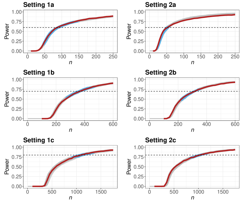
Figure 2: 100 local power curve approximations (semi-opaque grey), power curve estimated via simulated data (red), and target power $\Gamma$ (dotted line) for each setting. The probable domain of each prior-adjusted SSSD returned by Algorithm 2 is given in blue.

For all settings considered, our power curves generally provide a good local approximation near the target power: they yield reasonable sample size recommendations if we want the Bayesian equivalence test to have power of roughly $\Gamma$. The quality of the approximation appears to deteriorate slightly as we increase or decrease from $\Gamma$ in setting 2a. This setting considers a major adjustment to incorporate prior information; the sample sizes that achieve power of $\Gamma=0.6$ are respectively $n=89$ and 53 before and after this adjustment. The approximate power curve reasonably accounts for this, even though the power curves have slightly different shapes before and after adjusting for the priors. To better approximate a different portion of the power curve, our two-stage method could be implemented with a different target power $\Gamma$. Moderate and minor adjustments for the prior distributions are made in settings 2b and 2c, respectively.

The probable domain for the prior-adjusted SSSD that defined each approximation to the power curve is given in blue. If the blue lines were to not cover the horizontal dotted lines at the target power $\Gamma$, it would imply that the final sample size recommendation is not in the probable domain of the SSSD. In those cases, we may be able to obtain better results by anchoring our approximation to the power curve around an alternative sample size to $\tilde{\mu}_{l}$. The blue lines generally intersect the horizontal dotted lines for all settings in our numerical study. The alignment between the grey and red curves for the settings with uninformative priors also corroborates that the approach for fast power curve approximation proposed in Section 4.2 is suitable in situations where the BvM theorem can be reasonably applied.

We reiterate that each of the grey curves in Figure 2 can be estimated in roughly 5 seconds without parallelization. With the same computational resources for this example, we can approximate a couple of posteriors using sampling-resampling methods and not even one posterior using MCMC. This is not sufficient to produce even a crude power estimate for a single sample size $n$. Our method for sample size determination therefore allows users to quickly explore potential designs for their study. They can discard unrealistic designs that yield unattainable sample sizes in real time, expediting communication between stakeholders of the equivalence study.

7 Discussion

In this paper, we developed a framework for sample size determination with Bayesian equivalence tests facilitated via posterior probabilities. This framework is founded on the approximate normality of the SSSD, and we proposed a two-stage method to estimate this distribution. The numerical studies conducted show that our fast method yields suitable SSSD estimation and local power curve approximation for moderate and large sample sizes. While this method is not appropriate for small sample sizes, it informs practitioners when their required sample sizes are small. More traditional simulation-based design methods can be used in these scenarios since they are often less cumbersome to implement with small sample sizes.

It may be possible to make this framework more flexible by extending it to the predictive approach for choosing the sampling distribution of $\boldsymbol{Y}^{{}_{(n)}}$. This would prevent us from directly applying the BvM theorem. However, perhaps results from the BvM theorem (where we treat a draw from the design prior as the fixed parameter $\boldsymbol{\eta}_{j,0}$) could be combined with low-discrepancy sampling techniques to yield fast sample size recommendations. This framework could also be extended to accommodate multiple study objectives. For instance, we may require a sample size $n$ that both satisfies a power criterion and bounds a type I error or false discovery rate.

Moreover, the framework presented in the main paper does not support imbalanced two-group sample size determination (i.e., where $n_{2}=qn_{1}$ for some constant $q>0$). It may be inefficient or impractical to force $q=1$ when prior information for one group is much more precise, when it is more difficult to sample from one of the groups, or in scenarios where one treatment is much riskier. In Appendix D.2 of the supplement, we extend this framework to settings where practitioners specify this constant $q$.

Supplementary Material

These materials include a detailed description of the conditions for Theorem 1, along with additional simulation results and theoretical exposition. The code to implement our two-stage procedure and conduct the numerical studies in the main paper is available online: https://github.com/lmhagar/SSSD.

Funding Acknowledgement

This work was supported by the Natural Sciences and Engineering Research Council of Canada (NSERC) by way of CGS M and PGS D scholarships as well as Grant RGPIN-2019-04212.

References

- Adcock (1997) Adcock, C. (1997). Sample size determination: a review. Journal of the Royal Statistical Society: Series D (The Statistician) 46(2), 261–283.
- Berry et al. (2011) Berry, S. M., B. P. Carlin, J. J. Lee, and P. Muller (2011). Bayesian Adaptive Methods for Clinical Trials. CRC press.
- Brent (1973) Brent, R. P. (1973). An algorithm with guaranteed convergence for finding the minimum of a function of one variable. Algorithms for Minimization without Derivatives, Prentice-Hall, Englewood Cliffs, NJ, 61–80.
- Brutti et al. (2014) Brutti, P., F. De Santis, and S. Gubbiotti (2014). Bayesian-frequentist sample size determination: a game of two priors. Metron 72(2), 133–151.
- Chaloner (1996) Chaloner, K. (1996). Elicitation of prior distributions. In Bayesian biostatistics, pp. 141–156. Marcel Dekker, New York.
- De Santis (2007) De Santis, F. (2007). Using historical data for Bayesian sample size determination. Journal of the Royal Statistical Society: Series A (Statistics in Society) 170(1), 95–113.
- De Santis and Pacifico (2004) De Santis, F. and M. P. Pacifico (2004). Two experimental settings in clinical trials: predictive criteria for choosing the sample size in interval estimation. In Applied Bayesian statistical studies in biology and medicine, pp. 109–130. Springer.
- Garthwaite et al. (2005) Garthwaite, P. H., J. B. Kadane, and A. O’Hagan (2005). Statistical methods for eliciting probability distributions. Journal of the American Statistical Association 100(470), 680–701.
- Gelman et al. (2013) Gelman, A., J. B. Carlin, H. S. Stern, D. B. Dunson, A. Vehtari, and D. B. Rubin (2013). Bayesian Data Analysis. CRC press.
- Gilbert and Varadhan (2016) Gilbert, P. and R. Varadhan (2016). numderiv: Accurate numerical derivatives. R package version 8(1).