Search for Isocurvature with Large-scale Structure: A Forecast for Euclid and MegaMapper using EFTofLSS

Abstract

Isocurvature perturbations with a blue power spectrum are one of the natural targets for the future large scale structure observations which are probing shorter length scales with greater accuracy. We present a Fisher forecast for the Euclid and MegaMapper (MM) experiments in their ability to detect blue isocurvature perturbations. We construct the theoretical predictions in the EFTofLSS and bias expansion formalisms at quartic order in overdensities which allows us to compute the power spectrum at one loop order and bispectrum at tree level and further include theoretical error at the next to leading order for the covariance determination. We find that Euclid is expected to provide at least a factor of few improvement on the isocurvature spectral amplitude compared to the existing Planck constraints for large spectral indices while MM is expected to provide about 1 to 1.5 order of magnitude improvement for a broad range of spectral indices. We find features that are specific to the blue isocurvature scenario including the leading parametric degeneracy being with the Laplacian bias and a UV sensitive bare sound speed parameter.

Contents

1. I Introduction
2. II Mixed power spectrum scenario
3. III The EFTofLSS with isocurvature
   1. III.1 Peculiar counterterm property associated with the large spectral index
4. IV Galaxy power spectrum and bispectrum model
5. V UV divergences and correction
6. VI Parameter set and fiducial values
   1. VI.1 Surveys
   2. VI.2 Fiducial parameter values
7. VII Results and Discussion
8. VIII Conclusion
9. A Renormalization scheme
10. B Galaxy one-loop contributions
11. C Semi-analytic expression for $c_{{\rm ren,MX}}^{2}$
12. D Fisher matrix and theoretical error covariance
13. E Comparison to Halofit

I Introduction

Cold dark matter (CDM) isocurvature perturbations with a strongly blue spectral tilt can be completely negligible on large scales and be the dominant primordial inhomogeneity component on small length scales. Cosmic microwave background (CMB) strongly constrains the large scales and is currently the dominant anchor of standard cosmology (Planck:2015fie, ; Planck:2018jri, ), but future large scale structure surveys are poised to exceed the constraining power of the CMB on short length scales (Sailer:2021yzm, ). In this paper, we give a Fisher forecast of the constraining power of Euclid (Euclid, ) and MegaMapper (MM) (Schlegel:2019eqc, ) on strongly blue tilted isocurvature spectra.

CDM blue isocurvature perturbations are naturally generated in axion-like scenarios when the Peccei-Quinn symmetry breaking radial field is out of equilibrium during inflation (Kasuya:2009up, ). The duration of the time that the radial field is not at the minimum of the effective potential determines the $k$ range over which the spectrum is blue, with the spectral index being determined by the logarithmic time derivative of the radial field. In the overdamped radial dynamics, the spectrum is typically characterized by an approximately constant spectral index until the break point when the spectrum becomes flat again. While the overdamped scenario has only a mild bump at the break point (Chung:2016wvv, ), the underdamped scenarios can generate spectacular features near the break point that can include oscillations of huge amplitudes (Chung:2021lfg, ). In the present work, we consider a simplified version of these more physically complete scenarios by restricting to a single power law characterized by an amplitude and a spectral index.

For the theoretical cosmological fluid model that will be used to compute experimental observables, we use the EFTofLSS formalism (Baumann:2010tm, ) at one-loop order because it provides a principled way to control uncertainties from unknown small-scale physics in the spectral range of interest. We calibrate the counterterm of EFTofLSS using a combination of codes CLASS-PT (CLASS_PT, ), FastPM (Feng:2016yqz, ), and nbodykit (Hand:2017pqn, ). We model the galaxy counts using a bias expansion (Desjacques_2018, ) and compute the galaxy power spectrum at one-loop order and the bispectrum at tree-level. We include theoretical error estimates for the covariance determination using the higher-order error envelopes as given in (Baldauf:2016sjb, ; Chudaykin:2019ock, ).

We find that Euclid can give a factor of a few improvement on the isocurvature spectral amplitude constraint over that from the CMB for large isocurvature spectral indices ($n_{\mathrm{iso}}\gtrsim 3$), while MM can give more than an order of magnitude improvement for a broad range of $n_{\mathrm{iso}}$. The controlling factor in the degree of constraint is the signal data volume, and most of the signal (at the perturbative order used in this work) is coming from the power spectrum and not the bispectrum for these experiments, although bispectrum signal helps to break some parameter degeneracies. We identify the dominant source of signal degradation to come from the marginalization associated with the Laplacian bias due to a degeneracy of high spectral indexed blue isocurvature spectra with this Laplacian bias $k$-dependence.

One feature of the strongly blue isocurvature scenario in the EFTofLSS formalism that we uncover is that the bare sound speed parameter $c^{2}$ is both cutoff dependent and may even become negative when the cutoff is taken above $\Lambda\gtrsim O(3)$ Mpc^-1 for sizable isocurvature amplitudes. This does not significantly affect the analysis because the renormalized $c_{\mathrm{ren}}^{2}$ is of the same approximate value as in the case of the adiabatic scenarios. Along a similar theme, the one loop contributions to the galaxy power spectrum have integrals that are UV-sensitive ($\Lambda$-dependent) for high spectral indices. Again, we have enough bias parameter renormalization degree of freedom to absorb the UV sensitivities and marginalize, such that these peculiarities do not strongly affect the Fisher forecast in practice.

The order of presentation is as follows. In Sec. II, we parameterize the mixed (adiabatic + isocurvature) linear input power spectra. We review the EFTofLSS formalism in Sec. III and discuss the one-loop EFTofLSS parameterization used for the forecast. Here we also discuss the enhanced UV-sensitivity of the loop integrals coming from the large spectral index of the linear isocurvature power spectrum. In Sec. IV, we present the bias expansion used to model the galaxy power spectrum and bispectrum. Sec. V discusses the divergences and the renormalization procedure in the bias expansion. In Sec. VI, we give the assumed characteristics associated with the Euclid and MM experiments as well as the fiducial parameter set associated with the cosmology. We discuss the results in Sec. VII where the Euclid and MM sensitivity to strongly blue isocurvature spectra is presented. We conclude the paper in Sec. VIII with a summary of main results and an outlook of future related work.

The set of appendices that follow present some of the technical details. In App. A, the renormalization scheme used in this paper is defined. We list the one loop integrals appearing in the bias expansion in App. B. App. C gives the renormalized $c^{2}$ for the mixed case as a function of $z$ obtained by matching with N-body simulations. For a self-contained presentation, we review the Fisher forecast formalism and list our simplifying assumptions in App. D. In App. E we discuss how the current version of Halofit Takahashi:2012em is insufficient to describe the nonlinear power spectrum for the mixed initial condition scenarios.

II Mixed power spectrum scenario

We work in the standard 6-parameter $\Lambda$CDM cosmology with the addition of axion dark matter component with isocurvature initial conditions (ICs). Axion-like scenarios can naturally generate a large spectral tilt (strongly blue) CDM isocurvature perturbations when the Peccei-Quinn symmetry breaking radial field is out of equilibrium during inflation (Kasuya:2009up, ). The existence of a break in the spectrum is generic and required for the observability of the spectrum (Chung:2015tha, ). Furthermore, different initial conditions can lead to a rich set of dynamics that is seen in the features of the spectrum (Chung:2016wvv, ; Chung:2021lfg, ). In the case where the break point of the spectrum is far beyond $k_{\mathrm{NL}}$, we expect the perturbative observables to be sensitive mainly to the power law part of the blue spectrum. Hence, deferring a more complete analysis to a future work, we consider a simplified scenario in this paper and parameterize the primordial curvature and isocurvature spectra as the following standard power-law expressions (by introducing the dimensionless power spectrum $\Delta_{X}^{2}(k)=k^{3}P_{X}(k)/\left(2\pi^{2}\right)$)

$$\frac{k^{3}}{2\pi^{2}}P_{\mathcal{R}}(k)=A_{{\rm ad}}(k_{\mathrm{p}})\left(\frac{k}{k_{\mathrm{p}}}\right)^{n_{\mathrm{ad}}-1},\qquad\frac{k^{3}}{2\pi^{2}}P_{\mathcal{S}_{cdm}}(k)=A_{{\rm iso}}(k_{\mathrm{p}})\left(\frac{k}{k_{\mathrm{p}}}\right)^{n_{\mathrm{iso}}-1}$$ (1)

at a pivot scale $k_{{\rm p}}=0.05\,{\rm Mpc^{-1}}$. Since axionic theories give $1\leq n_{{\rm iso}}\leq 4$ in the scaling part of the spectrum, we restrict our $n_{{\rm iso}}$ to this range. We also assume that the curvature-isocurvature cross-correlation is negligible which corresponds to a situation where the axion coupling to the inflaton is sufficiently suppressed. Due to the linearity of first order perturbation theory, the general mixed perturbations evolve as a linear superposition of the adiabatic (AD) and isocurvature (ISO) components that evolve independently and hence the total linear matter power spectrum in presence of both adiabatic and CDM-isocurvature fluctuations (mixed (MX) state) can be given as

$$P_{{\rm lin}}^{{\rm MX}}(k,z\ll z_{{\rm eq}}) =P_{{\rm lin}}^{{\rm{\rm AD}}}(k,z)+P_{{\rm lin}}^{{\rm ISO}}(k,z).$$ (2)

This then allows us to write the linear power spectrum at the time when the perturbative loop expansion will be made as

$$P_{{\rm lin}}^{{\rm MX}}(k,z\ll z_{{\rm eq}}) =P_{{\rm lin}}^{{\rm{\rm AD}}}(k,z)\left(1+\alpha\left(\frac{f_{c}}{3}\right)^{2}\left(\frac{T_{{\rm iso}}(k)}{T_{{\rm ad}}(k)}\right)^{2}\left(\frac{k}{k_{\mathrm{p}}}\right)^{n_{{\rm iso}}-n_{{\rm ad}}}\right)$$ (3)

where

$$\alpha=\frac{A_{{\rm iso}}(k_{{\rm p}})}{A_{{\rm ad}}(k_{{\rm p}})}$$ (4)

and $f_{c}$ is the fraction of cold dark matter (CDM) energy density over total dark matter and baryon energy density assuming that the primordial isocurvature mode is generated within CDM fluctuations. The additional factor of $\left(1/3\right)^{2}$ is obtained by mapping superhorizon isocurvature modes to curvature perturbations during Matter-Dominated (MD) era due to the change in the effective sound speed-squared $c_{s}^{2}$. The transfer functions $T_{{\rm iso}}(k)$ and $T_{{\rm ad}}(k)$ are standard linear transfer functions associated with the $\Lambda$CDM cosmology. By construction, $T\rightarrow 1$ as $k\rightarrow 0$ (for very large scales) whereas it decreases monotonically at small scales. The actual shape dependence of $T(k)$ relies upon the primordial mode (adiabatic or isocurvature) sourcing the fluctuations where isocurvature modes suffer from additional small scale suppression compared to adiabatic since they are characterized as initial zero energy density or potential modes (1986ApJ, ; Efstathiou:1986pba, ).

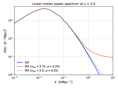
Figure 1: Plot showing a comparison between the linear matter power spectra at a redshift of $z=2$ for the pure adiabatic and mixed initial conditions. For the mixed case, we use fiducial values as $\alpha=0.25$ and plot two curves for $n_{\mathrm{iso}}=3.75$ (dashed) and $n_{\mathrm{iso}}=3.0$ (dotted).

To illustrate the comparison between the two initial conditions, in Fig. 1 we plot linear matter power spectrum at a redshift of $z=2$ generated from the CLASS code (Blas:2011rf, ) for the pure adiabatic and mixed initial conditions. To gain a perspective into the magnitude of $\alpha$, we note that latest Planck analysis constraints $\alpha\lesssim O(0.1)$ (Planck:2018jri, ) at $k_{{\rm p}}$ which implies that $P_{{\rm lin}}^{{\rm ISO}}(k_{{\rm p}})\lesssim O(0.01)P_{{\rm lin}}^{{\rm AD}}(k_{{\rm p}})$. Hence, isocurvature power is roughly $O\left(1\%\right)$ or less than adiabatic on large scales.

III The EFTofLSS with isocurvature

In this work we use the EFTofLSS to model the galaxy power spectrum and bispectrum observables on perturbative non-linear scales. Although cosmic emulators such as (Moran:2022iwe, ), seem to fit the numerical simulations well for the adiabatic case over a wide range for the cosmological parameters, the current versions are not trained for mixed isocurvature and are also subject to baryonic uncertainty. The semi-analytical Halofit approach (Takahashi:2012em, ) to clustering also fails when one includes isocurvature perturbations, as we briefly explore in App. E. On the other hand, the EFTofLSS (Baumann:2010tm, ; Carrasco_2012, ; Ivanov:2022mrd, ) has a well-defined expansion parameter that controls errors and can be extended to include isocurvature. The EFT approach models UV-effects/backreaction of small-scale non-linear physics through various unknown free parameters whose values are determined from simulations.

EFTofLSS in the mixed case has a mild disadvantage compared to the adiabatic case because of the relatively larger variation in the counterterm fitting parameter such as renormalized $c^{2}$ with the changes in the isocurvature model parameters. This is because the blue isocurvature spectrum becomes large on small scales, which critically affects the UV behavior of the theory. However, because of the degeneracy of these parameters with the bias parameters and because the theory error is dominated by the next order term in the loop expansion, this variation in the counterterm parameters does not play a significant role in the current analysis.

In the present forecast, we will consider our theoretical model for power spectrum and bispectrum by including all contributions up to quartic power in linear matter overdensity, $O\left(\left(\delta^{(1)}\right)^{4}\right)$, where throughout our analysis we will assume Gaussian initial conditions such that $\left\langle\delta^{(1)}\right\rangle=0$. At this order in perturbative expansion, we can at most work with one-loop galaxy power spectrum and tree-level bispectrum (Angulo:2015eqa, ). As we will see, this is sufficient to see a signal in the experiments that we forecast.

As done in (Carrasco_2012, ), one can expand the non-linear matter overdensity perturbatively to one-loop as

$$\delta=\delta^{(1)}+\delta^{(2)}+\delta^{(3)}+\delta^{(c_{1})}+\epsilon_{{\rm m}}$$ (6)

where $\delta^{(1,2,3)}$ are effectively Standard Perturbation Theory (SPT (Bernardeau:2001qr, )) solutions (i.e. $\delta_{{\rm SPT}}\approx\delta^{(1)}+\delta^{(2)}+\delta^{(3)}$ to third order in $\delta^{(1)}$), and $\delta^{(c_{1})}$ and $\epsilon_{{\rm m}}$ are the one-loop counterterm and stochastic noise term. More specifically, the terms $\delta^{(c_{1})}+\epsilon_{{\rm m}}$ represent the corrections in the EFTofLSS arising from residual pressure sources associated with averaging the Euler equation, where these sources have been expanded in powers of derivatives and $\delta^{(1)}$ with the expansion coefficients ( such as $c^{2}$) parameterized instead of being computed. This parameterization allows an introduction of a $\Lambda$-dependent coefficient that can be used to remove the $\Lambda$-dependence in the observable correlator. The often called stochastic term $\epsilon_{{\rm m}}$ is defined to be independent of $\delta^{(1)}$ such that its contribution is uncorrelated with $\delta^{(n)}$, e.g. $\left\langle\delta^{(1)}\epsilon_{{\rm m}}\right\rangle=0$. Using this expansion, the following standard expression for the non-linear power spectrum is derived in (Carrasco_2012, ) as

$$P_{{\rm NL}}(k,z)=P_{{\rm 11}}(k,z)+\left[P_{{\rm 22}}(k,z)+P_{13}(k,z)\right]+P_{{\rm ctr}}(k,z)+P_{\Delta\tau}(k,z),$$ (7)

where $P_{{\rm 11}}\equiv P_{{\rm lin}}$ is the linear matter power spectrum, and that $P_{{\rm 12}}(k,z)$ vanishes due to our assumption of Gaussian initial conditions. In the EFTofLSS , although the quantity $P_{11}$ is the power spectrum of the fields smeared over length scales shorter than $\Lambda^{-1}$, because $P_{11}$ is evaluated at $k\ll\Lambda$, we approximate $P_{11}$ as the unsmeared power spectrum.

The one-loop contributions $P_{22}$ and $P_{13}$ are given by the expressions

$$P_{22}(k)=2\int_{q}F_{2}^{2}\left(\bar{q},\bar{k}-\bar{q}\right)P_{{\rm 11}}(q)P_{{\rm 11}}(|\bar{k}-\bar{q}|),$$ (8)

$$P_{13}(k)=6P_{{\rm 11}}(k)\int_{q}F_{3}\left(\bar{q},-\bar{q},\bar{k}\right)P_{{\rm 11}}(q),$$ (9)

where $\int_{q}\equiv\int\frac{d^{3}q}{\left(2\pi\right)^{3}}$ and $\bar{k}=\bar{q}_{1}+...+\bar{q}_{n}$. The explicit expressions for the standard SPT convolution kernels $F_{2,3}$ are given in (Bernardeau_2002, ) whereas simplified loop integrals useful for all evaluations can be found in (Carrasco_2012, ; Senatore:2014via, ). The SPT expressions for $P_{22}$ and $P_{13}$ in Eqs. (8) and (9) are correct only in an Einstein de-Sitter (EdS) universe where momentum and time-dependence of the convolution loop integrals decouple. However, it is a common approach to use EdS based kernels $F_{2,3}$ even in non-EdS spacetimes and subsequently replace the linear growth function, $D_{+}(z)$, consistent with non-EdS cosmologies because the momentum addition deformations are not as important as the scaling from the growth function. This approach has been tested analytically Takahashi:2008yk and with a number of N-body simulations (Baldauf_2015, ) and found to be very accurate such that the residual difference is negligible for foreseeable future surveys.

The counterterm at the one-loop order (coming from $\left\langle\delta^{(c_{1})}\delta^{(1)}\right\rangle$) is conveniently represented as

$$P_{{\rm ctr}}(k,z)=-2c^{2}(z)k^{2}P_{11}(k,z)$$ (10)

where $c^{2}$ is an effective parameter arising from the parameterization of $\delta^{(c_{1})}$ . The higher order $k$ terms not shown in Eq. (10) will represent higher than 4th perturbative order since we can view $k^{2}$ as second order in $k/k_{\mathrm{NL}}$ and $P_{{\rm 11}}(k,z)\propto\left(\delta^{(1)}\right)^{2}$ as second perturbative order. The parameter $c^{2}$ models the effective sound speed-squared that arises due to the gravitational clustering induced by small-scale fluctuations (Carrasco_2012, ; Baldauf_2015, ). It is noteworthy that the spectral shape of the contribution in Eq. 10 also accounts for the leading order effects from baryonic physics on large-scales Lewandowski:2014rca , because total matter over-density $\delta$ is sum of cdm and baryonic contributions. These effects are most important post star-formation and their contribution is modeled effectively through the modification of the parameter $c^{2}$. As we shall note in Sec. IV, the degeneracy of $c^{2}$ with the Laplacian bias parameter $b_{\nabla^{2}\delta}$ implies we can effectively account for these by treating Laplacian bias as a free nuisance parameter. In practice, $c^{2}$ is determined by matching Eq. (7) to numerical simulations. If $P_{13}$ is divergent with a cutoff dependent term having the same $k$ functional form as Eq. (10), then $c^{2}$ is necessarily divergent (i.e. cutoff dependent) and its non-divergent piece after combining with $P_{13}$ is the observationally relevant “renormalized” piece, which we will call $c_{{\rm ren}}^{2}$ : i.e. we can rewrite Eq. (7) as

$$P_{{\rm NL}}(k,z) =P_{{\rm 11}}(k,z)+P_{{\rm 22}}(k,z)+\left(P_{13}(k,\Lambda,z)-2c_{{\rm\Lambda}}^{2}(k_{\rm{ren}},\Lambda,z)k^{2}P_{{\rm 11}}(k,z)\right)$$

$$-2c_{{\rm ren}}^{2}(k_{\rm{ren}},z)k^{2}P_{{\rm 11}}(k,z)+P_{\Delta\tau}(k,z)$$ (12)

where $P_{11}$ and $P_{22}$ have a weak cutoff dependence for $k\ll\Lambda$, and $c_{{\rm\Lambda}}^{2}(k_{\rm{ren}},\Lambda,z)$ will have the cutoff dependence to cancel the divergent (UV-sensitive) part of the $P_{13}$ term. From dimensional analysis, one would expect the parameter $c_{\mathrm{ren}}^{2}(k_{\rm{ren}},z)$ to be of order $\sim 1/k_{{\rm NL}}^{2}$. In the present work, we use CLASS code (Blas:2011rf, ) to generate the linear power spectra which is input to FastPM (Feng:2016yqz, ) whose N-body output phase space data is processed by nbodykit (Hand:2017pqn, ) to generate the nonlinear power spectra to compute $c_{{\rm ren}}^{2}$. In Fig. 2 we show examples of the one-loop EFT matter power spectrum fitted to the N-body simulations obtained from FastPM for both adiabatic and mixed ICs. The curves are plotted for redshifts $z=1$ and $z=2$. The $k_{\rm{reach}}$ which we define as the smallest mode where the EFT curve deviates by more than $1.5\%$ from N-body data is $\approx$ $0.5\leavevmode\nobreak\$h/Mpc ($0.65\leavevmode\nobreak\$h/Mpc) at redshift $z=1$ ($z=2$) respectively.

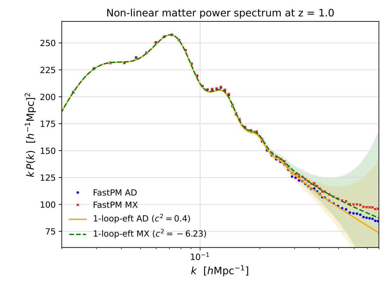
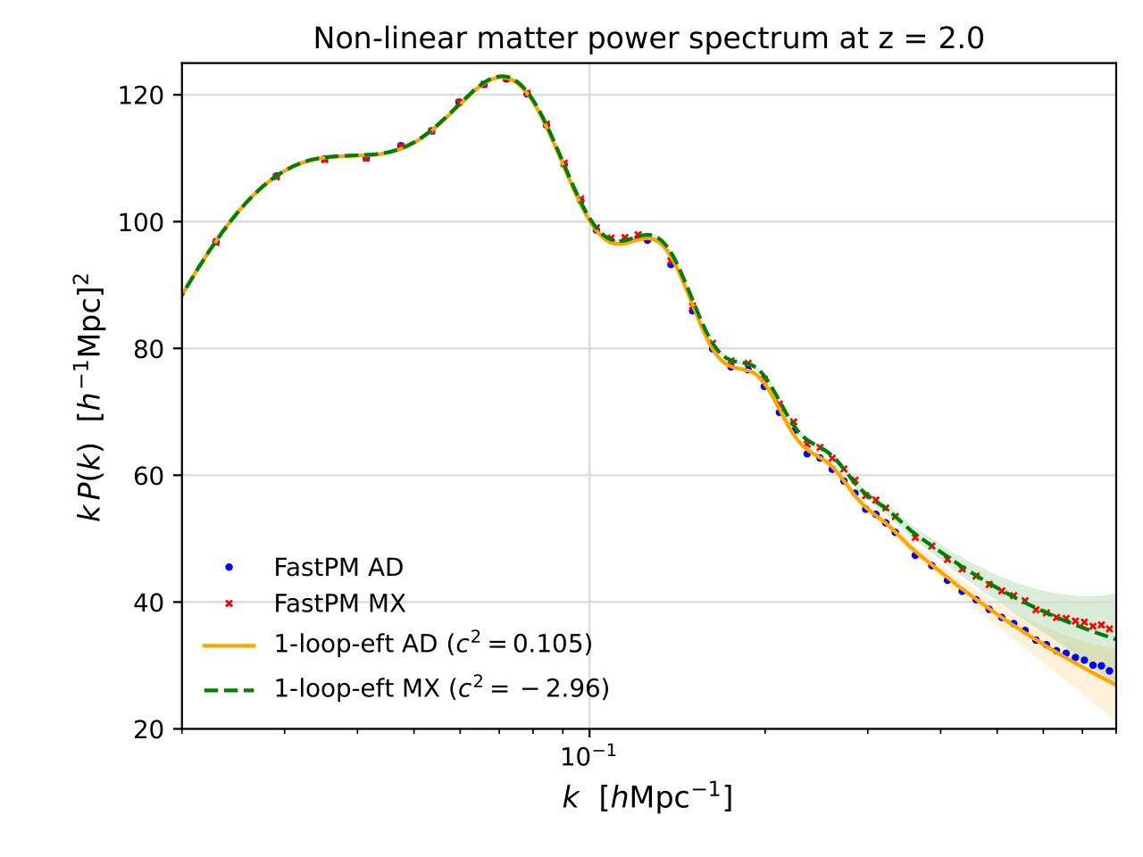
Figure 2: In this figure we highlight the fitting of one-loop EFT power spectrum to the N-body data from FastPM Feng:2016yqz . Note that we plot scaled power spectrum, $k\times P(k)$, on the y-axis for clarity. For the mixed case, we use fiducial values as $n_{\rm{iso}}=3.75$ and $\alpha=0.25$. The value of the bare $c^{2}$ (at cutoff $\Lambda=100$ h/Mpc) one-loop EFT parameter is given in the label for the EFT curves. Note that the value of $c^{2}$ for the mixed case is negative. We discuss this peculiarity in Sec. III.1. The $k_{\mathrm{reach}}$ of the one-loop EFT curves is $\approx$ $0.5\leavevmode\nobreak\$h/Mpc ($0.65\leavevmode\nobreak\$h/Mpc) at redshift $z=1$ ($z=2$). We also plot approximate theoretical error band expected from two-loop contributions (see Eq. (27). As can be seen in the plots, the two-loop error estimate is quite conservative. See Fig. 1 to compare with the corresponding linear power spectra. In Appendix E we discuss comparison of N-body results with Halofit and CosmicEmu.

The additional contribution $P_{\Delta\tau}$ is obtained by the two-point function of $\epsilon_{m}\sim k^{2}\Delta\tau$ where $\Delta\tau$ has an intuitive interpretation of residual effective pressure coming from the smearing operation. Unlike $P_{{\rm ctr}}$, the stochastic term $P_{\Delta\tau}$ scales as $k^{4}$ but is found to be negligible for the purposes of our analysis because of the following argument. We know $\Delta\tau$ has the magnitude of pressure, which means that the two-point function of $\Delta\tau$ in $k$ space has a natural magnitude of pressure squared divided by $k_{{\rm NL}}^{3}$. The appearance of $k_{{\rm NL}}^{3}$ signals that this object originates from short distances. This estimate leads to

$$\frac{P_{\Delta\tau}(k)}{c_{{\rm ren}}^{2}(k_{\rm{ren}},z)k^{2}P_{{\rm 11}}(k,z)}\sim\left(\frac{k}{k_{{\rm NL}}}\right)^{2-n}$$ (13)

where $n\approx-1.5$ parameterizes the $k$ scaling of the dimensionful power spectrum near $k\sim 0.1h$/Mpc. Since on $k/k_{\mathrm{NL}}\sim O(0.1)$, the suppression is expected to be $O(10^{-3})$ which allows us to drop this term from further analysis.

III.1 Peculiar counterterm property associated with the large spectral index

Interestingly within the literature, one often takes the integration cutoff $\Lambda\rightarrow\infty$ since the $P_{13}$ integral is finite for pure adiabatic ICs and the associated parameter $c^{2}=c_{\Lambda}^{2}+c_{{\rm ren}}^{2}$ is also finite (Carrasco_2012, ; Hertzberg_2014, ). Accordingly, the often quoted value of sound speed $c^{2}(z=0;\Lambda\rightarrow\infty)\sim O(1)\;{\rm\left(Mpc/h\right)^{2}>0}$ is a bare value which is directly measured from N-body simulations/data (Carrasco_2012, ; Carrasco:2013sva, ; Hertzberg_2014, ; Foreman:2015lca, ; Baldauf_2015, ; Baldauf:2015tla, ; Angulo:2015eqa, ; Foreman:2015uva, ). However, this approach is unsuitable when studying a wide range of mixed blue-isocurvature ICs with two additional free model parameters, $n_{{\rm iso}}$ and $\alpha$. The UV part of $P_{13}$ integral which can be written as

$$P_{13}^{{\rm UV}}(k,\Lambda)\approx-k^{2}P_{{\rm 11}}(k)\frac{61}{630\pi^{2}}\int^{\Lambda}dqP_{{\rm 11}}(q)$$ (14)

is divergent for primordial isocurvature spectra with $n_{{\rm iso}}\gtrsim 3$. Since this term is combined with the counterterm Eq. (10) containing the $c^{2}$ coefficient to produce a finite term, $c^{2}$ does not converge as $\Lambda\rightarrow\infty$. Although one can still measure the bare parameter $c^{2}$ directly from N-body simulations, a direct comparison with the adiabatic scenario is not particularly meaningful given that the parameters in the two cases have different interpretations. For instance unlike the adiabatic case, if $n_{{\rm iso}}=3.75$ and $\alpha=0.25$, the bare value $c^{2}\left({\rm Mpc/h}\right)^{-2}$ has a magnitude of $O(-20)$ as $\Lambda$ goes to $O(100{\rm h/Mpc})$ at a redshift of $z=0$. In Fig. 2 we plotted EFT curves obtained for mixed ICs with negative value of fitted $c^{2}$ parameter at different redshifts. Although this negative value may naively seem alarming, this coefficient merely represents a coefficient of an EFT operator consistent with symmetries and power counting, and we did not make assumptions of positivity of this coefficient.

More importantly, we note that the only IR-surviving quantity inherited from the UV effects is the renormalized parameter $c_{{\rm ren}}^{2}$. Hence, we compare the renormalized parameter $c_{{\rm ren}}^{2}(k_{\rm{ren}},z)$ (instead of the bare parameter) between different cosmological scenarios while keeping $\Lambda\gg O(10)k_{\mathrm{NL}}$ arbitrary. In Fig. 3 we plot the difference in the value of renormalized sound speed squared parameter between mixed and pure adiabatic ICs obtained at a renormalization scale $k_{{\rm ren}}=0.1\rm{h/Mpc}$ by matching the EFTofLSS one-loop perturbation theory to the N-body simulations. The renormalized value $c_{{\rm ren,AD}}^{2}\left(k_{{\rm ren}}=0.1{\rm h/Mpc}\right)$ at $z=0$ for pure adiabatic ICs is $\approx 14{\rm\left(Mpc/h\right)^{2}}\sim 1/k_{{\rm NL}}^{2}$ for $k_{{\rm NL}}\approx 0.3{\rm h/Mpc}$. Compared to a large difference between the bare $c^{2}$ parameters, the difference, $\Delta c_{{\rm ren}}^{2}=c_{{\rm ren,MX}}^{2}-c_{{\rm ren,AD}}^{2}$, of the renormalized value for the two ICs is $\approx\left(5-10\right)\%$ for high blue spectral indices and with a sizable isocurvature fraction, $\alpha\sim O(0.1)$. In Appendix C we discuss and give a semi-analytical empirical fitting function for $c_{{\rm ren,MX}}^{2}-c_{{\rm ren,AD}}^{2}$ for values of $O(0.01)\lesssim\alpha<1$ and $2\leq n_{{\rm iso}}\leq 4$ for redshifts $z\leq 2$.

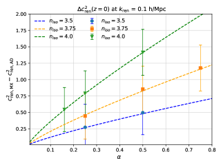
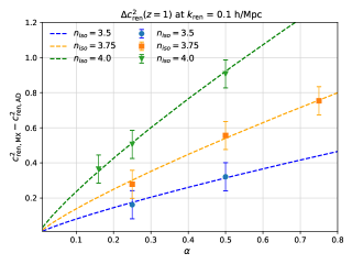
Figure 3: Plot showing the difference in the renormalized value of the effective sound speed squared $c_{{\rm ren}}^{2}$ between mixed and pure ICs obtained by fitting Eq. (12) to the numerical data from N-body simulations at $z=0$ and $1$. Additionally, we also plot (dashed curves) a semi-analytical empirical fitting formula derived in Appendix C. Note that the estimation of $c_{{\rm ren}}^{2}$ from N-body data at higher redshifts has smaller error bars since the number of modes available for fitting (with smaller cosmic variance and theoretical error) increases with $z$. Note that the error bars in this figure are given by cosmic variance and set an upper limit on the true statistical error. We have used phase-matched simulations to determine $c^{2}$, which means that the AD and MX simulations have the same random seeds. This procedure cancels cosmic variance (see e.g. Villaescusa-Navarro:2018bpd for a discussion) such that the true statistical error bars should be significantly smaller.

In order to see the effect of a change in the value of renormalized fluid parameter, we take the ratio

$$\frac{\Delta P_{c_{{\rm ren}}}(k,z)}{P_{11}(k,z)}=2\Delta c_{{\rm ren}}^{2}(k_{\rm{ren}},z)k^{2}\\ =\frac{2\Delta c_{{\rm ren}}^{2}(k_{\rm{ren}},z)}{100}\left(\frac{k}{0.1}\right)^{2}$$ (16)

which says that an $O(1)$ change in $\Delta c_{{\rm ren}}^{2}$ can result in a $>1\%$ deviation in the non-linear matter power spectrum at $k>0.1{\rm h/Mpc}$. This is consistent with the results of Fig. 3. Therefore, when requiring high precision theoretical perturbative matter power spectrum for mixed ICs with $\alpha\sim O(0.1)$, we propose using the semi-analytic empirical fitting function for high blue spectral indices. However, for small isocurvature amplitudes, $\alpha\lesssim O(0.01)$, it is sufficient to take $c_{{\rm ren,MX}}^{2}\approx c_{{\rm ren,AD}}^{2}$. Additionally, when working with the biased tracers like galaxy/halo power spectrum, we note that the one-loop renormalized fluid parameter $c_{{\rm ren}}^{2}$ is degenerate with the $b_{\nabla^{2}\delta}$ bias coefficient, as we will discuss more below. In forecasts of experiments that do not break this degeneracy, a precise value of $c_{{\rm ren}}^{2}$ is not required since we marginalize over the bias parameters. In the present work, it will thus be adequate to work with the renormalized EFT or bias parameters of adiabatic ICs and apply them directly to the analysis/forecasts for mixed IC cosmologies.

IV Galaxy power spectrum and bispectrum model

We use the one-loop galaxy power spectrum and tree-level bispectrum obtained through a bias expansion for the galaxy density contrast by including all operators allowed by Galilean symmetry up to cubic order in magnitude as the coarse-grained linear overdensity $\delta_{\Lambda}^{(1)}$ (Desjacques_2018, ),

$$\delta_{g}(x) =\sum_{\mathcal{O}}\left(b_{\mathcal{O}}+\epsilon_{\mathcal{O}}(x)\right)\mathcal{O}(x)+b_{\epsilon}\epsilon(x)$$ (17)

$$=b_{1}\delta(x)+b_{\epsilon}\epsilon(x)$$

$$+\frac{b_{2}}{2}\delta^{2}(x)+b_{\mathcal{G}_{2}}\mathcal{G}_{2}(x)+\epsilon_{\delta}(x)\delta(x)$$

$$+b_{\delta\mathcal{G}_{2}}\delta(x)\mathcal{G}_{2}(x)+\frac{b_{3}}{6}\delta^{3}(x)+b_{\mathcal{G}_{3}}\mathcal{G}_{3}(x)+b_{\Gamma_{3}}\Gamma_{3}(x)+\epsilon_{\delta^{2}}(x)\delta^{2}(x)+\epsilon_{\mathcal{G}_{2}}(x)\mathcal{G}_{2}(x)$$

$$+b_{\nabla^{2}\delta}\nabla^{2}\delta(x)+b_{\nabla^{2}\epsilon}\nabla^{2}\epsilon(x)$$ (18)

where all the operators $\mathcal{O}$ in the above expression are considered to be coarse-grained and the subscript $\Lambda$ is dropped for brevity. In Fourier space the Laplacian takes the form $\nabla^{2}\rightarrow\left(k/k_{*}\right)^{2}$ where $k_{*}$ is some characteristic scale of clustering for biased tracers and we restrict to scales $k/k_{*}\ll 1$. Hence every insertion of a Laplacian is equivalent to a second order correction to an operator $\mathcal{O}$ and the derivative operators in the last-line of Eq. (18) are counted approximately as cubic order in bias expansion. Therefore, Eq. (18) is a double expansion in density fluctuations and their derivatives. The remaining operator set $\{\delta^{2},\mathcal{G}_{2},\epsilon_{\delta}\delta\}$ and $\{\mathcal{G}_{2}\delta,\delta^{3},\mathcal{G}_{3},\Gamma_{3},\epsilon_{\delta^{2}}\delta^{2},\epsilon_{\mathcal{G}_{2}}\mathcal{G}_{2}\}$ are second and third order respectively where we refer the readers to (Assassi:2014fva, ; Desjacques_2018, ) for definition and details regarding these operators.

Notably (Chan_2012, ) and (Assassi:2014fva, ) have shown that operators non-local in $\delta$ such as $\mathcal{G}_{2}=\left(\nabla_{i}\nabla_{j}\Phi\right)^{2}-\left(\nabla^{2}\Phi\right)^{2}$ arise naturally due to gravitational evolution and renormalization requirements respectively. Meanwhile, $\epsilon$ in Eq. (18) is the stochastic noise contribution to the galaxy formation where we remark that the stochastic fields $\epsilon_{{\rm m}}$, $\epsilon$ and $\epsilon_{\mathcal{O}}$ (here the stochastic operators $\epsilon_{\mathcal{O}}$ are sourced through gravitational evolution) are modeled such that they are sourced by small-scale fluctuations and are assumed to be uncorrelated with the long-wavelength perturbative fluctuations at large separations.

One can choose the renormalization condition (see (Assassi:2014fva, ) and (Desjacques_2018, ) for details regarding the field-redefinition procedure which we summarize in Appendix A) such that the one-loop galaxy power spectrum at $O\left(\left(\delta^{(1)}\right)^{4}\right)$ can be written as

$$P_{gg}(k) =b_{1}^{2}P_{{\rm NL}}(k)+P_{gg}^{{\rm NLO}}(k)+P_{gg,\nabla^{2}\delta}(k)+P_{gg,\epsilon}(k)$$ (19)

where the non-linear matter power spectrum up to one-loop in the EFTofLSS perturbation theory is given as

$$P_{{\rm NL}}(k)=P_{11}(k)+P_{22}(k)+P_{13}(k)-2c^{2}k^{2}P_{11}(k)$$ (20)

and the next-to-leading order one-loop contributions (without stochastic terms) are given by

$$P_{gg}^{{\rm NLO}}(k) =b_{1}\left(b_{2}\mathcal{I}_{\delta^{(2)}\delta^{2}}(k)+2b_{\mathcal{G}_{2}}\mathcal{I}_{\delta^{(2)}\mathcal{G}_{2}}(k)+\left(2b_{\mathcal{G}_{2}}+\frac{4}{5}b_{\Gamma_{3}}\right)\mathcal{F}_{\mathcal{G}_{2}}(k)(k)\right)$$

$$+b_{2}b_{\mathcal{G}_{2}}\mathcal{I}_{\delta^{2}\mathcal{G}_{2}}(k)+\frac{1}{4}b_{2}^{2}\mathcal{I}_{\delta^{2}\delta^{2}}(k)+b_{\mathcal{G}_{2}}^{2}\mathcal{I}_{\mathcal{G}_{2}\mathcal{G}_{2}}(k)$$ (21)

where the loop contributions $\mathcal{I}_{\mathcal{O},\mathcal{O}^{\prime}}(k)$ are given in Appendix B. The leading derivative contribution is

$$P_{gg,\nabla^{2}\delta}(k)=-2b_{1}b_{\nabla^{2}\delta}\left(\frac{k}{k_{*}}\right)^{2}P_{{\rm 11}}(k)$$ (22)

and the stochastic noise contribution is given as

$$P_{gg,\epsilon}(k)=P_{\epsilon\epsilon}b_{\epsilon}\left(1+2b_{\nabla^{2}\epsilon}\left(\frac{k}{k_{{\rm*}}}\right)^{2}\right).$$ (23)

Note that all these quantities were computed after renormalizing the composite operators such as $\delta^{2}$ with the renormalization scheme explained in Appendix A. Contributions from other operators like $\delta^{3},\mathcal{G}_{3},\delta\mathcal{G}_{2}$ do not appear as they are eliminated in the renormalization scheme used in this paper (see Appendix A). The bias term associated with the parameter $b_{\nabla^{2}\epsilon}$ represents a scale-dependent deviation from a purely Poissonian shot noise (i.e. the $k^{2}$ dependence makes this scale dependent instead of being a constant), and represents a (small) correlation of the stochastic bias on large scales. Depending upon the value of $b_{\nabla^{2}\epsilon}$ it can either enhance or reduce the total power spectrum (Eggemeier_2020, ; Eggemeier_2021, ). As we will discuss more in depth later, the scale $k_{*}$ in Eq. (23) is close to the nonlinear scale $k_{{\rm NL}}.$ In Sec. V we will note that the higher-derivative stochastic bias term is also motivated by the renormalization requirements for the next-to-leading order (NLO) terms.

Due to the assumed Gaussian initial conditions of $\delta_{k_{1}}^{(1)}$, the galaxy bispectrum at the perturbative order $O\left(\left(\delta^{(1)}\right)^{4}\right)$ is given by the following terms (Scoccimarro_2004, ):

$$B_{gg}\left(\vec{k}_{1},\vec{k}_{2},\vec{k}_{3}\right) \sim b_{1}^{3}\left\langle\delta_{k_{1}}^{(1)}\delta_{k_{2}}^{(1)}\delta_{k_{3}}^{(2)}\right\rangle$$

$$+b_{1}^{2}b_{2}\left\langle\delta_{k_{1}}^{(1)}\delta_{k_{2}}^{(1)}\delta_{k_{3}}^{2}\right\rangle+b_{1}^{2}b_{\mathcal{G}_{2}}\left\langle\delta_{k_{1}}^{(1)}\delta_{k_{2}}^{(1)}\mathcal{G}_{2k_{3}}\right\rangle$$

$$+b_{1}^{2}\left\langle\delta_{k_{1}}\delta_{k_{2}}\left(\epsilon_{\delta}\delta\right)_{k_{3}}\right\rangle+\left\langle\epsilon_{k_{1}}\epsilon_{k_{2}}\left(\epsilon_{\delta}\delta\right)_{k_{3}}\right\rangle+b_{1}\left\langle\epsilon_{k_{1}}\delta_{k_{2}}\left(\epsilon_{\delta}\delta\right)_{k_{3}}\right\rangle+\left\langle\epsilon_{k_{1}}\epsilon_{k_{2}}\epsilon_{k_{3}}\right\rangle+\mbox{permutations }$$ (24)

where the terms in the last line give a mixed stochastic noise contribution and the vectors $\vec{k}_{1,2,3}$ must form a closed triangle such that $\vec{k}_{1}+\vec{k}_{2}+\vec{k}_{3}=0.$ Note that the stochastic contributions represent $k>k_{\mathrm{NL}}$ contributions to the perturbations which generically will be non-Gaussian. Evaluating the three-point correlation functions we obtain

$$B_{gg}\left(\vec{k}_{1},\vec{k}_{2},\vec{k}_{3}\right) =\left(F_{2}^{b}\left(\vec{k}_{1},\vec{k}_{2}\right)b_{1}^{2}P_{11}(k_{1})P_{11}(k_{2})+\mbox{cyclic}\right)$$

$$+P_{{\rm shot}}\sum_{i=1}^{3}b_{1}^{2}P_{11}(k_{i})+B_{{\rm shot}}$$ (25)

where

$$F_{2}^{b}\left(\vec{k}_{1},\vec{k}_{2}\right)=\frac{b_{2}}{2}+b_{\mathcal{G}_{2}}\left(\mu_{12}^{2}-1\right)+b_{1}\left(\frac{5}{7}+\frac{1}{2}\mu_{12}\left(\frac{k_{1}}{k_{2}}+\frac{k_{2}}{k_{1}}\right)+\frac{2}{7}\mu_{12}^{2}\right)$$ (26)

for $\mu_{12}=\vec{k}_{1}\cdot\vec{k}_{2}/\left(k_{1}k_{2}\right)$, and $P_{{\rm shot}}$ and $B_{{\rm shot}}$ are the shot noise contributions whose fiducial values will be discussed in Sec. VI.2. At the perturbative order $\left(\delta^{(1)}\right)^{4}$, the galaxy bispectrum in Eq. (25) is given only by tree-level terms since unlike the power spectrum in Eq. (19) it does not contain any loop corrections. Also we point out that the only relevant bias terms at this order for bispectrum are $b_{1},b_{2}\mbox{, and }b_{\mathcal{G}_{2}}$.

For the theoretical error estimates we consider the following explicit two-loop error envelope $E_{{\rm gg}}(k,z)$ for the galaxy-galaxy power spectrum as given in (Chudaykin:2019ock, ):

$$E_{{\rm gg}}^{{\rm p}}(k,z)=\left(D_{+}(z)/D_{+}(0)\right)^{4}P_{{\rm gg}}(k,z)\left(\frac{k}{0.45\,{\rm hMpc^{-1}}}\right)^{3.3}$$ (27)

where $P_{{\rm gg}}$ is the galaxy auto-correlation power spectrum at one-loop order without the stochastic component. We would like to emphasize that the error envelope provided in Eq. 27 is a conservative estimate of the actual error, typically by a factor of $\sim 2$ compared to DM simulations for the majority of the relevant k-values. However, given that this estimate is derived from matching with DM-only N-body simulations and considering the possibility of larger errors in the case of biased tracers, we find it appropriate to still apply this estimate to the biased tracer measurements. Overall, a more accurate estimation of the theoretical error specifically for the biased tracers holds the potential for better forecast and fitting results in future analyses. In this regard, we refer the readers to DAmico:2019fhj , where the authors conducted a systematic analysis to estimate the theory errors from Mock galaxy samples. We also remark that we have verified the above error envelope for mixed isocurvature scenarios and found it to be in good agreement (see Fig. 2). This can be partially explained by the smallness of the isocurvature contribution $\alpha(f_{c}/3)^{2}\ll 1$ (see Eq. (3)) allowed by the existing data in the $k$-range that the present forecast experiments are sensitive to and the stability of the error envelope to small perturbations. Similarly, for the tree-level bispectrum we approximate the error envelope with

$$E_{{\rm gg}}^{{\rm b}}(k,z)=3\left(D_{+}(z)/D_{+}(0)\right)^{2}B_{{\rm gg}}(k,z)\left(\frac{k_{t}/3}{0.31\,{\rm hMpc^{-1}}}\right)^{1.8}$$ (28)

where $B_{{\rm gg}}(k,z)$ is now the tree-level bispectrum (without $B_{{\rm shot}}$) evaluated using Eq. (25) and $k_{{\rm t}}=\left|\vec{k}_{{\rm 1}}+\vec{k}_{{\rm 2}}+\vec{k}_{{\rm 3}}\right|$.

V UV divergences and correction

Similar to the discussion in Sec. III where we reviewed the need to renormalize the loop integrals in the matter power spectrum, the next to leading order $P_{gg}^{{\rm NLO}}$ terms (Eq. (21)) in the galaxy two-point correlation function may also show similar $\Lambda$-dependence and UV divergences. Specifically, the one-loop terms in Eq. (21) have the following UV limits

$$\lim_{k\rightarrow 0}\mathcal{I}_{\delta^{(2)}\delta^{2}}(k) =\frac{-1}{42\pi^{2}}k^{2}\int^{\Lambda}dq\left(P_{11}(q)\right)^{2}+O(k^{4}),$$

$$\lim_{k\rightarrow 0}\mathcal{I}_{\delta^{(2)}\mathcal{G}_{2}}(k) =\frac{-1}{21\pi^{2}}k^{4}\int^{\Lambda}dq\left(\frac{P_{11}(q)}{q}\right)^{2}+O(k^{6}),$$

$$\lim_{k\rightarrow 0}\mathcal{F}_{\mathcal{G}_{2}}(k) =-\frac{16}{21\pi^{2}}k^{2}P_{11}(k)\int^{\Lambda}dqP_{11}(q)+O(k^{4}),$$

$$\lim_{k\rightarrow 0}\mathcal{I}_{\delta^{2}\delta^{2}}(k) =\frac{1}{2\pi}\int^{\Lambda}dq\left(qP_{11}(q)\right)^{2}+\frac{k^{2}}{4\pi^{2}}\int^{\Lambda}dqP_{11}(q)\left(\frac{4}{3}q\partial_{q}P_{11}(q)+\frac{2}{3}q^{2}\partial_{q}^{2}P_{11}(q)\right)+O(k^{4}),$$

$$\lim_{k\rightarrow 0}\mathcal{I}_{\mathcal{G}_{2}\mathcal{G}_{2}}(k) =\frac{8}{15\pi^{2}}k^{4}\int^{\Lambda}dq\left(\frac{P_{11}(q)}{q}\right)^{2}+O(k^{6}),$$

$$\lim_{k\rightarrow 0}\mathcal{I}_{\delta^{2}\mathcal{G}_{2}}(k) =\frac{-2}{3\pi^{2}}k^{2}\int^{\Lambda}dq\left(P_{11}(q)\right)^{2}+O(k^{4}).$$ (29)

In the limit $k/\Lambda\rightarrow 0$, we expect the galaxy power spectrum to be well-defined by the leading perturbative term associated with the linear bias and a stochastic field $\epsilon$. Hence all higher order bias terms should become insignificant at very large scales. One notes from Eq. set (29) that the leading $O(k^{0})$ contribution from $\mathcal{I}_{\delta^{2}\delta^{2}}(k)$ term does not vanish as $k/\Lambda\rightarrow 0$. Since it is clear that any $O(k^{0})$ quantity will be degenerate with the stochastic contribution $b_{\epsilon}^{2}\left\langle\epsilon_{k}\epsilon_{p}\right\rangle$, we remove the $\Lambda$-dependent $O(k^{0})$ diverging contribution from $\mathcal{I}_{\delta^{2}\delta^{2}}(k)$ by subtracting the $k/\Lambda\rightarrow 0$ leading term $\frac{1}{2\pi}\int^{\Lambda}dq\left(qP_{11}(q)\right)^{2}$ from $\mathcal{I}_{\delta^{2}\delta^{2}}(k)$ and redefining the stochastic bias parameter $b_{\epsilon}$ in Eq. (23) to absorb this contribution. Hence, the first renormalized $\mathcal{I}_{\delta^{2}\delta^{2}}$ is written as

$$\mathcal{I}_{\delta^{2}\delta^{2}}^{{\rm[R1]}}(k)\equiv\mathcal{I}_{\delta^{2}\delta^{2}}(k)-\frac{1}{2\pi}\int_{0}^{\Lambda}dq\left(qP_{11}(q)\right)^{2}=\frac{k^{2}}{4\pi^{2}}\int_{0}^{\Lambda}dqP_{11}(q)\left(\frac{4}{3}q\partial_{q}P_{11}(q)+\frac{2}{3}q^{2}\partial_{q}^{2}P_{11}(q)\right)+O(k^{4}).$$ (30)

where only $k^{2}$ independent term has been removed and thus not fully renormalized. This freedom to absorb the contact terms by explicitly reparameterizing the stochastic bias parameters was first emphasized in (PhysRevD.74.103512, ) and also noted in (Senatore:2014eva, ; Assassi:2014fva, ). After this procedure, we find that all one-loop contributions in $P_{gg}^{{\rm NLO}}$ scale as either $k^{2}$ or $k^{4}$ in the limit $k\rightarrow 0$. For the general pure adiabatic ICs, the correction made above to the $\mathcal{I}_{\delta^{2}\delta^{2}}(k)$ one-loop term is sufficient to ensure that all the one-loop integrals in Eq. (21) converge and thus vanish in the limit $k\rightarrow 0$. One can see this explicitly in (Simonovic:2017mhp, ) which gives a range of spectral index-related parameters $\nu\in\left(\nu_{\mbox{IR}},\nu_{\mbox{UV}}\right)$ for which the integrals converge. For pure adiabatic ICs in $\Lambda{\rm CDM}$ characterized by near-scale-invariance, it is easy to check that the one-loop integrals in Eq. set (29) are convergent as $q\rightarrow\infty$, and the terms vanish in the limit $k\rightarrow 0$ due to an overall $k^{n}$ scaling. However, we note that similar to $P_{13}$ loop term, the integral $\mathcal{F}_{\mathcal{G}_{2}}(k)$ has a finite non-negligible support from non-linear scales $q\sim q_{{\rm NL}}$ and thus includes contribution from scales where our perturbation theory is known to be inaccurate. This naively worrisome inaccuracy however does not contribute to the physical observables as their contributions are absorbed by the renormalization scheme used for $b_{\nabla^{2}\delta}$.

Unlike the case for pure adiabatic ICs, the UV sensitivity for mixed ICs with large blue spectral indices is more severe since the one-loop terms $\mathcal{I}_{\delta^{(2)}\delta^{2}}(k)$, $\mathcal{I}_{\delta^{2}\delta^{2}}^{{\rm[R1]}}(k)$ and $\mathcal{I}_{\delta^{2}\mathcal{G}_{2}}(k)$ are UV divergent when $n_{{\rm iso}}\gtrsim 3.5$ and $\mathcal{F}_{\mathcal{G}_{2}}(k)$ is divergent when $n_{{\rm iso}}\gtrsim 3$. We note that the leading UV behavior of $\mathcal{I}_{\delta^{(2)}\delta^{2}}(k)$, $\mathcal{I}_{\delta^{2}\delta^{2}}^{{\rm[R1]}}(k)$ and $\mathcal{I}_{\delta^{2}\mathcal{G}_{2}}(k)$ correspond to contact terms of the form $O(k^{n})$ for $n\geq 2$ and are absorbed by the renormalization condition of higher order derivatives of stochastic terms in our bias expansion. For instance, the bias term $b_{\nabla^{2}\epsilon}$ in Eq. (23) is redefined after absorbing all $O(k^{2}\times\mbox{constant})$ contact terms. This will be part of our renormalization scheme for the bias expansion. Likewise, the leading divergent piece from $\mathcal{F}_{\mathcal{G}_{2}}(k)$ which scales as $O\left(k^{2}P_{11}(k)\right)$ is removed by redefining the $b_{\nabla^{2}\delta}$ bias parameter of the leading higher-derivative operator. These are shape-changing contributions and are often interpreted as scale-dependent additions to the linear bias $b_{1}$.

Finally, the new renormalized one-loop terms in $P_{gg}^{{\rm NLO}}$ are given as

$$\mathcal{I}_{\delta^{(2)}\delta^{2}}^{{\rm[R]}}(k) = \mathcal{I}_{\delta^{(2)}\delta^{2}}(k)-\frac{1}{2\pi}\int_{0}^{\Lambda}dq\left(qP_{11}(q)\right)^{2}-C_{\delta^{(2)}\delta^{2}}k^{2},$$

$$\mathcal{I}_{\delta^{2}\delta^{2}}^{{\rm[R]}}(k) = \mathcal{I}_{\delta^{2}\delta^{2}}(k)-2\int_{q}P_{{\rm 11}}(q)P_{{\rm 11}}(q)-C_{\delta^{2}\delta^{2}}k^{2},$$

$$\mathcal{I}_{\delta^{2}\mathcal{G}_{2}}^{{\rm[R]}}(k) = \mathcal{I}_{\delta^{2}\mathcal{G}_{2}}(k)-C_{\delta^{2}\mathcal{G}_{2}}k^{2},$$

$$\mathcal{F}_{\mathcal{G}_{2}}^{{\rm[R]}}(k) = \mathcal{F}_{\mathcal{G}_{2}}(k)-C_{\mathcal{F}_{\mathcal{G}_{2}}}k^{2}P_{11}(k),$$

$$\mathcal{I}_{\delta^{(2)}\mathcal{G}_{2}}^{{\rm[R]}}(k) = \mathcal{I}_{\delta^{(2)}\mathcal{G}_{2}}(k),$$

$$\mathcal{I}_{\mathcal{G}_{2}\mathcal{G}_{2}}^{{\rm[R]}}(k) = \mathcal{I}_{\mathcal{G}_{2}\mathcal{G}_{2}}(k),$$ (31)

where the $\Lambda$-dependent coefficients $C_{\mathcal{O},\mathcal{O}^{\prime}}$ are given by the following expressions

$$C_{\delta^{(2)}\delta^{2}} \equiv\frac{1}{2}\left.\frac{d^{2}\mathcal{I}_{\delta^{(2)}\delta^{2}}(k)}{dk^{2}}\right|_{k=0}=-\frac{1}{42\pi^{2}}\int_{0}^{\Lambda}dq\left(P_{11}(q)\right)^{2},$$ (32)

$$C_{\delta^{2}\delta^{2}} \equiv\frac{1}{2}\left.\frac{d^{2}\mathcal{I}_{\delta^{2}\delta^{2}}(k)}{dk^{2}}\right|_{k=0}=\frac{1}{4\pi^{2}}\int_{0}^{\Lambda}dqP_{11}(q)\left(\frac{4}{3}q\partial_{q}P_{11}(q)+\frac{2}{3}q^{2}\partial_{q}^{2}P_{11}(q)\right),$$ (33)

$$C_{\delta^{2}\mathcal{G}_{2}} \equiv\frac{1}{2}\left.\frac{d^{2}\mathcal{I}_{\delta^{2}\mathcal{G}_{2}}(k)}{dk^{2}}\right|_{k=0}=\frac{-2}{3\pi^{2}}\int_{0}^{\Lambda}dq\left(P_{11}(q)\right)^{2},$$ (34)

$$C_{\mathcal{F}_{\mathcal{G}_{2}}} \equiv\frac{1}{P_{11}(k)}\frac{1}{2}\left.\frac{d^{2}\mathcal{F}_{\mathcal{G}_{2}}(k)}{dk^{2}}\right|_{k=0}=-\frac{16}{21\pi^{2}}\int_{0}^{\Lambda}dqP_{11}(q).$$ (35)

After subtracting the $C_{\mathcal{O},\mathcal{O}^{\prime}}$ dependent pieces, the renormalized one-loop contributions (except $\mathcal{F}_{\mathcal{G}_{2}}^{{\rm[R]}}(k)$) have the same $O(k^{4}$) behavior on large scales, which are subdominant to other contributions. The leading $O(k^{0}$) and $O(k^{2})$ contributions are now carried by the stochastic terms associated with the renormalized biases $b_{\epsilon}$ and $b_{\nabla^{2}\epsilon}$. Similarly, the leading $O(k^{2}P_{11}(k))$ contributions are controlled by the EFT parameter $c_{{\rm ren}}^{2}$ and the Laplacian bias parameter $b_{\nabla^{2}\delta}$, leading to a parametric degeneracy with respect to the galaxy correlation function observable at the quartic order in our bias expansion. However, these degeneracies are broken when bispectrum, redshift-space distortion (RSD) effects and/or matter and tracer cross-correlation power spectrum are included in the set of observables. Using the expressions given in Eq. set (31), it is easy to check that the power spectra for the pure adiabatic and mixed (adiabatic and blue isocurvature) ICs are equivalent at large scales ($k\rightarrow 0$) for any arbitrary value of the cutoff scale $\Lambda$. This is what we expect on long wavelengths where the adiabatic contributions dominate.

Finally, the complete galaxy power spectrum up to one-loop order is given by the following set of bias parameters

$$\left\{b_{1},b_{2},b_{\mathcal{G}_{2}},b_{\Gamma_{3}},b_{\nabla^{2}\delta},b_{\epsilon},b_{\nabla^{2}\epsilon}\right\}$$ (36)

and the corresponding one-loop contributions are given in Eq. set (31). Note that $\{b_{\epsilon},b_{\nabla^{2}\delta},b_{\nabla^{2}\epsilon}\}$ are $\Lambda$-dependent. When we marginalize over these parameters in the numerical procedure, we are marginalizing over only the finite pieces that are left over after canceling the $\Lambda$-dependent pieces. We will call the parameters after the subtraction discussed above as $\{b_{\epsilon}^{[R]},b_{\nabla^{2}\delta}^{[R]},b_{\nabla^{2}\epsilon}^{[R]}\}$.

For example, the galaxy power spectrum has a contribution

$$P_{gg}(k) \supset b_{1}\left(2b_{\mathcal{G}_{2}}+\frac{4}{5}b_{\Gamma_{3}}\right)\mathcal{F}_{\mathcal{G}_{2}}(k)-2b_{1}b_{\nabla^{2}\delta}\left(\frac{k}{k_{*}}\right)^{2}P_{{\rm 11}}(k)$$

where $\mathcal{F}_{\mathcal{G}_{2}}(k)$ is divergent as $\Lambda/k_{\mathrm{NL}}\rightarrow\infty$. This divergent piece can be subtracted as

$$b_{1}\left(2b_{\mathcal{G}_{2}}+\frac{4}{5}b_{\Gamma_{3}}\right)\mathcal{F}_{\mathcal{G}_{2}}(k)-2b_{1}b_{\nabla^{2}\delta}k^{2}P_{{\rm 11}}(k) =b_{1}\left(2b_{\mathcal{G}_{2}}+\frac{4}{5}b_{\Gamma_{3}}\right)\left(\mathcal{F}_{\mathcal{G}_{2}}(k)-C_{\mathcal{F}_{\mathcal{G}_{2}}}k^{2}P_{11}(k)\right)$$

$$-2b_{1}\left(b_{\nabla^{2}\delta}-\left(b_{\mathcal{G}_{2}}+\frac{2}{5}b_{\Gamma_{3}}\right)C_{\mathcal{F}_{\mathcal{G}_{2}}}\right)k^{2}P_{{\rm 11}}(k)$$ (37)

$$=b_{1}\left(2b_{\mathcal{G}_{2}}+\frac{4}{5}b_{\Gamma_{3}}\right)\mathcal{F}_{\mathcal{G}_{2}}^{[{\rm R}]}(k)-2b_{1}b_{\nabla^{2}\delta}^{[{\rm R}]}k^{2}P_{{\rm 11}}(k)$$ (38)

where $C_{\mathcal{F}_{\mathcal{G}_{2}}}$ is defined in Eq. (35), and we defined the renormalized Laplacian bias as

$$b_{\nabla^{2}\delta}^{[{\rm R}]}=b_{\nabla^{2}\delta}-\left(b_{\mathcal{G}_{2}}+\frac{2}{5}b_{\Gamma_{3}}\right)C_{\mathcal{F}_{\mathcal{G}_{2}}}.$$ (39)

It is this type of renormalized parameter such as $b_{\nabla^{2}\delta}^{[{\rm R}]}$ that will be marginalized over in the forecast. As mentioned earlier in Sec. III, we will evaluate the renormalized counterterm and bias parameters for adiabatic ICs and use them directly for forecasts related to mixed ICs.

VI Parameter set and fiducial values

In this section, we present the relevant experimental characteristics for Euclid (Euclid, ) and MegaMapper (Schlegel:2019eqc, ) that we use in our forecast. For a detailed discussion on these two and several other futuristic high-redshifts surveys, we refer the reader to (Sailer:2021yzm, ). We also list the fiducial parameter values, errors used, marginalized parameters, and other assumptions made in the Fisher forecast.

VI.1 Surveys

The Euclid satellite (planned for launch in 2023) will measure star-forming luminous galaxies containing ${\rm H\alpha}$ emitters using a near-infrared telescope (Euclid, ; Euclid:2019clj, ). The satellite is expected to map nearly 15,000 square degrees of sky probing a redshift range up to $z\sim 2$. In order to model the expected population density of ${\rm H\alpha}$ emitters at high-redshifts, we consider its redshift distribution per solid-angle $dN(z)/d\Omega dz$ by averaging the data given in (Pozzetti:2016cch, ) and (Euclid:2019clj, ). Integrating this distribution over the surveyed area and a redshift bin yields $N(\bar{z})$, the expected number of galaxies to be detected.

Similar to the analysis in (Chudaykin:2019ock, ), we will consider 6 non-overlapping redshift bins with the corresponding mean galaxy number densities $n(\bar{z})=N(\bar{z})/V(\bar{z})$ provided in Table 1. We evaluate the comoving volume $V(\bar{z})$ of a redshift bin centered around $\bar{z}$ using the expression

$$V(\bar{z})=\frac{4\pi}{3}\left(r_{\bar{z}+\Delta z/2}^{3}-r_{\bar{z}-\Delta z/2}^{3}\right)$$ (40)

where $r_{z}$ is the comoving distance up to a redshift of $z$. Note that the surveyed volume $V_{s}(z)=V(z)f_{{\rm sky}}$ where we will set the fraction of sky surveyed $f_{{\rm sky}}\approx 0.35$ for both Euclid and MegaMapper. For each redshift bin centered at $\bar{z}$, we set the fiducial linear bias parameter for Euclid surveyed galaxy samples as $b_{1}=\sqrt{1+\bar{z}}$ (Euclid:2021qvm, ).

$\bar{z}$	0.8	1.0	1.2	1.4	1.6	1.8
$n(\bar{z})$[$10^{-3}{\rm h^{3}Mpc^{-3}}]$	2.08	1.18	0.7	0.42	0.26	0.19

Table 1: Mean galaxy number density $n(\bar{z})=N(\bar{z})/V(\bar{z})$ expected to be measured by the Euclid survey at a given redshift bin centered at $\bar{z}$ for 6 non-overlapping redshift bins of width $\Delta z=0.2$.

$\bar{z}$	2.0	3.0	4.0	5.0
$n(\bar{z})$$[10^{-3}{\rm h^{3}Mpc^{-3}}]$	0.98	0.12	0.1	0.04

Table 2: ‘Fiducial’ mean galaxy number density $n(\bar{z})=N(\bar{z})/V(\bar{z})$ expected to be measured by MM at a given redshift bin centered at $\bar{z}$ for 4 non-overlapping redshift bins of width $\Delta z=1.0$.

While the Euclid survey is under construction and expected to be launched in 2023 providing us with a plethora of cosmological data for following 6 years, we will also give a forecast of a futuristic experiment, MegaMapper (MM) (Schlegel:2019eqc, ), that is still at the design stage. Similar to Euclid, MM will cover nearly 14,000 square degrees of the sky but surveying galaxies at higher redshift than Euclid ($2<z<5$) during an observation period of roughly 5 years. MM will primarily look for Lyman Break Galaxies (LBGs) to distinguish the higher redshift galaxies. For the forecast, we will consider the fiducial MM experiment consisting of $\approx 40$ million galaxies in the aforementioned redshift range for which the number density and redshift bins are listed in Table 2 of (Ferraro:2019uce, ) and also given in Tab. (2) here. We choose this fiducial case instead of the idealized case (see Table 1 of (Ferraro:2019uce, )) to be more conservative. These fiducial functions give a good fit to previous observations on large scales, where we expect the $b_{1}$ parameter to dominate. Note that the galaxy biases of Tables 1 and 2 of (Ferraro:2019uce, ) are magnitude dependent, in contrast with the bias parameters that would map smooth density fields to all galaxy counts. This feature is one of the contributing factors to the definition of fiducial and idealized. It is also interesting to note that Table 2 of (Ferraro:2019uce, ) has a non-monotonic behavior of $b_{1}(z)$ as it has a local maximum at $z\approx 3$. This feature seems to be partially responsible for features that we see in the redshift dependencies of various sensitivity plots in Sec. VII.

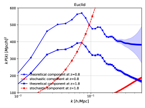
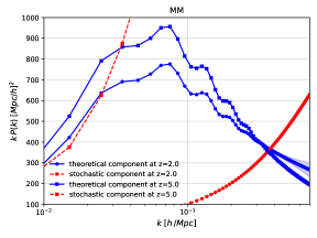
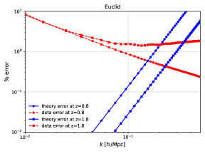
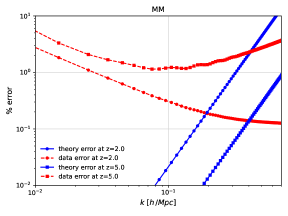
Figure 4: In the first row, we present plots showing the theoretical (solid, blue) and stochastic components (dashed, red) of the galaxy power spectrum for the Euclid and MM surveys at the first and last redshifts of their respective redshift ranges using fiducial bias parameters given in next subsection. For Euclid (figure on the left) we plot data at redshifts $z=0.8$ (circle marker) and $z=1.8$ (square marker). Similarly, for MM (figure on the right) we plot data at redshifts $z=2.0$ (circle marker) and $z=5.0$ (square marker). We also plot the theoretical error envelope as the ‘shaded’ region over the theoretical curve. In the second row, we plot the expected data and theory errors for the aforementioned redshifts using Eqs. (86) and (88) respectively. Note that the data error is dominated by cosmic variance (shot-noise) at low (high) k. The plots highlight that at the low redshifts, the signal-to-noise (S/N) is mainly constrained by the theoretical error rather than the stochastic component. At high redshifts, the signal is controlled by the stochastic component and bulk of the S/N is proportional to $b^{2}_{1}(z)n_{g}(z)$ (see Sailer:2021yzm for a plot of $b^{2}_{1}(z)n_{g}(z)$ for the two surveys considered here.)

In Fig. 4 we give plots of the theoretical galaxy power spectrum along with the expected stochastic component for the Euclid and MM surveys at the first and last redshifts for their respective redshift ranges aiming to highlight the factors affecting the expected signal. The signal-to-noise (S/N) ratio at each redshift primarily depends on two factors: the associated stochastic component, which is related to the number density of measured galaxies, and the theory error, which determines the reliability of theoretical estimates across different physical scales. When observing low redshifts with higher galaxy number densities, we anticipate that the S/N will be predominantly limited by the theoretical error. This observation is clearly evident in the plot shown on the left in the first row of Fig. 4. In the same figure, depicted in the second row, we present the expected data and theory errors by normalizing the square root of the data and theory covariances in Eqs. (86) and (88) with the theoretical power spectrum. We find that the signal is mostly negligible for scales where the theory errors exceed a few $\%$. Consequently, we set a definitive cutoff, denoted as $k_{\rm{cut}}$, for the Fisher analysis, where the theory error reaches $\approx 15\%$.

In our forecast we do not explicitly model redshift measurement errors, however for both Euclid and MegaMapper these should not strongly affect our forecast, which relies on perturbative scales (see e.g. Sailer:2021yzm for a discussion of redshift errors of these experiments). On the other hand, redshift space distortions (RSD) can affect our results and are not currently included in our forecast. We defer the inclusion of RSDs to future work.

VI.2 Fiducial parameter values

We set our baseline cosmological parameters to

$$A=1\hskip 24.0pt\Omega_{b}=0.0486\hskip 24.0pt\Omega_{c}=0.2589\hskip 24.0ptn_{s}=0.9667\hskip 24.0pth=0.6774$$ (41)

where $A=A_{{\rm s}}/A_{{\rm s,fid}}$ for $A_{{\rm s,fid}}=2.1413\times 10^{-9}$ and adopt uniform priors for these cosmological parameters from the latest Planck analysis (Planck:2018jri, ).

Having set the fiducial values of the linear bias $b_{1}$ for each survey as discussed in Sec. VI.1, we set the fiducial values of remaining bias parameters as follows. For quadratic and higher order tidal scalar biases, we consider a parametric form inspired from Lagrangian bias or co-evolution models (Chan_2012, ; Baldauf:2012hs, ; Eggemeier_2019, ):

$$b_{2}=\frac{8}{21}\left(b_{1}-1\right),\qquad b_{\mathcal{G}_{2}}=-\frac{2}{7}\left(b_{1}-1\right),\qquad b_{\Gamma_{3}}=\frac{23}{42}\left(b_{1}-1\right).$$ (42)

While the accuracy of the above functional form for setting up the fiducial values is formally less than what we are working with in the EFTofLSS , our final results (forecasts) are sufficiently insensitive to these choices due to the maginalization over the bias parameters. For instance, alternative fitting functions for quadratic bias $b_{2}$ obtained from N-body simulations and HOD modeling can be found in (Lazeyras:2015lgp, ; Yankelevich:2018uaz, ; DiDio:2018unb, ).

Additionally, we will make the standard assumption that the scale-independent stochastic contribution $b_{\epsilon}P_{\epsilon\epsilon}=P_{\rm{shot}}=1/\bar{n}_{g}$ and also set $B_{{\rm shot}}=1/\bar{n}_{g}^{2}.$ These control the number of modes that will contribute to our isocurvature signal of interest. If these numbers are larger, than the number of modes contributing to the signal decreases. The fiducial values are aligned with standard conservative practices, since detailed studies indicate the actual values may be a bit smaller at large scales for massive halos, while a positive correction can be expected for less massive halos (Baldauf:2013hka, ).

For the leading higher derivative and scale-dependent stochastic bias parameters, $b_{\nabla^{2}\delta}$ and $b_{\nabla^{2}\epsilon}$, respectively, we use the analysis of (Eggemeier_2020, ) and assume following fiducial values

$$b_{\nabla^{2}\delta}=-1$$ (43)

and

$$b_{\nabla^{2}\epsilon}=-0.2$$ (44)

with the clustering scale $k_{*}$ set as

$$k_{*}\approx k_{{\rm HD}}\approx 0.4\left(D_{+}(z)/D_{+}(0)\right)^{-4/3}\left({\rm h/Mpc}\right)$$ (45)

where ${\rm HD}$ subscript stands for “higher-derivative”. The particular choice of redshift dependence is motivated by a similar expression for $k_{{\rm NL}}$ obtained from linear dimensionless matter power spectrum. We note that the matter clustering scale $k_{*}$ need not have the same redshift dependence as the matter non-linear scale $k_{{\rm NL}}$ (Lazeyras:2019dcx, ). However, we have checked numerically that changing the redshift dependence does not change the forecast results for the isocurvature signal, mostly because we are marginalizing over the bias parameters. For simplicity, we will present the results with the redshift dependence of Eq. (45). We remark that the z-dependence of the fiducial value of the Laplacian bias differs from that of the non-Laplacian biases (such as $b_{1}$, $b_{2}$, $b_{\mathcal{G}_{2}}$, $b_{\Gamma_{3}}$, etc.), which have fiducial values inspired by the co-evolution models and thus scale as $\sqrt{1+z}\sim D_{+}(z)^{-0.5}$. Hence, unlike Laplacian biases, the fiducial values of the non-Laplacian biases increase with $z$. However, all non-Laplacian biases appear as prefactors of the one-loop terms given in Eq. 21 which have z-dependences given by the fourth power of growth function, $D_{+}(z)^{4}$. In contrast, the leading order Laplacian bias in Eq. 22 multiples the linear power spectrum which scales as $D_{+}(z)^{2}$. Consequently, the one-loop terms contain an additional quadratic power of the growth function. Thus, despite of the non-Laplacian biases increasing with $z$, the effective z-scaling (including biases) of the one-loop terms in Eq. 21 and the leading order Laplacian contribution in Eq. 22 is almost the same. Both of these terms vanish (become insignificant) on large scales at a similar rate at higher redshifts.

Finally, for the purposes of forecasting we will consider the following reduced set of nuisance parameters:

$$\{\mbox{nuisance}\}=\{b_{1},b_{2},b_{\mathcal{G}_{2}},b_{\nabla^{2}\delta},b_{\nabla^{2}\epsilon}\}$$ (46)

where we note that since the pair of bias parameters $\{b_{\mathcal{G}_{2}},b_{\Gamma_{3}}\}$ and $\{b_{1}c^{2},b_{\nabla^{2}\delta}\}$ are known to be highly degenerate, we do not include $b_{\Gamma_{3}}$ and $b_{1}c^{2}$ within our set of nuisance parameters over which we vary the likelihood function. The reason for the degeneracy of $\{b_{1}c^{2},b_{\nabla^{2}\delta}\}$ is small $k$ expansion, while the reason for the degeneracy of $\{b_{\mathcal{G}_{2}},b_{\Gamma_{3}}\}$ seems to be an accidental symmetry of the convolution existing at this order in perturbation theory. Hence, the Fisher matrix information does not include theoretical derivatives with respect to these two model parameters. We set Gaussian priors for the bias parameters with the standard deviations

$$\sigma_{b_{1}}=4,\quad\sigma_{b_{2}}=2,\quad\sigma_{b_{i}}=1$$ (47)

which apply to bias parameters in Eq. (46). Note that we do not include the prior for a bias when we marginalize over it.

For the Fisher analysis (see Appendix D for a review of Fisher forecast formalism), we set a coarse momentum bin width $k_{{\rm bin}}=0.01\,{\rm hMpc^{-1}}$ with $k_{\min}=0.005\,{\rm hMpc^{-1}}$ and error envelope correlation length $\Delta k=0.1\,{\rm hMpc^{-1}}$. We found that the results change by less than 10% to the choice of $\Delta k$ in the range $0.05-0.13\,{\rm hMpc^{-1}}$. We set the pivot scale at $k_{{\rm p}}=0.05\,{\rm Mpc^{-1}}$, following the Planck convention, such that the results for the ratio of the amplitude of the primordial isocurvature to adiabatic power spectrum $\alpha$ are given at $0.05\,{\rm Mpc^{-1}}$.

VII Results and Discussion

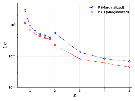
Figure 5: 1-$\sigma$ error forecast for an example isocurvature amplitude $\alpha=0.01$ and spectral index $n_{{\rm iso}}=3$, achievable by Euclid and MegaMapper (MM) as a function of the redshift reach. Here, the curves for $z\lesssim 2$ correspond to those for Euclid while the curves for $z\gtrsim 2$ correspond to those for MM, and for example the point at $z=$5 accounts for the information accumulated in the redshift range 2 to 5. The decrease in the error results from a combination of both the decreasing theoretical uncertainty as well as the increase in the number of modes available at higher redshifts (i.e. number of modes increase with $k_{\mathrm{max}}^{3}$ where $k_{\mathrm{max}}$ represents the maximum $k$-mode with sufficiently accurate theoretical predictions as well as with the number of redshift bins). The label $P$ denotes that the one-loop galaxy power spectrum and the label $B$ denotes the tree-level bispectrum are used in making the forecasts. Note that most of the constraining power comes from the power spectrum because of the limited number of modes available for the tree-level bispectrum compared to a one-loop power spectrum. The inclusion of the bispectrum signal helps to break the degeneracy (correlation) from $b_{1},b_{2},$ and $b_{\mathcal{G}_{2}}$ bias parameters and thus reduces the error by $\approx 20-30\%$ compared to a power spectrum only analysis.

Fig. 5 shows marginalized 1-$\sigma$ error sensitivity for the isocurvature amplitude, $\alpha$ , achievable by Euclid and MegaMapper experiments as a function of the redshift reach. Larger the redshift, more modes are available for the one-loop power spectrum since the error envelope is smaller at higher redshifts. The resulting cumulative signal sensitivity at higher redshifts is responsible for the decreasing error shown in the plot. We expect the error forecast to be smaller in magnitude in the idealized galaxy bias scenario as discussed below Table 2. Hence, this forecast should be seen as a conservative estimate, and we would realistically expect better results. Furthermore, since there is no RSD in the observables considered here, its inclusion can break the bias degeneracies and improve signal in a fuller analysis. (See (Chudaykin:2019ock, ) for a recent forecast on neutrino masses that highlights the improvement in error bars from RSD and AP effects.)

Most of the constraint/signal in Fig. 5 comes from the one-loop power spectrum due to the larger number of modes available compared to the tree-level bispectrum. However, the inclusion of the bispectrum signal helps to break the degeneracy (correlation) from $b_{1},b_{2},$ and $b_{\mathcal{G}_{2}}$ bias parameters to some extent and thus reduce the error by $\approx 20-30\%$ compared to a power spectrum only analysis. This is illustrated by ‘$\times$’ marked (red) curve. If the bispectrum computation is improved, then one would naively expect further significant improvements. However, because of the proliferation of the bias parameters at one-loop bispectrum level, there is a trade-off whose final effects to the error computation is not obvious (Eggemeier_2019, ; Philcox:2022frc, ). There is some previous work (Eggemeier_2021, ) which argues that these higher order bias contributions to the bispectrum can be fixed using co-evolution and peak background split relations ((Lazeyras:2015lgp, )) such that the required number of independent bias parameters is greatly reduced and thus do not completely degrade the gain from the improved accuracy.

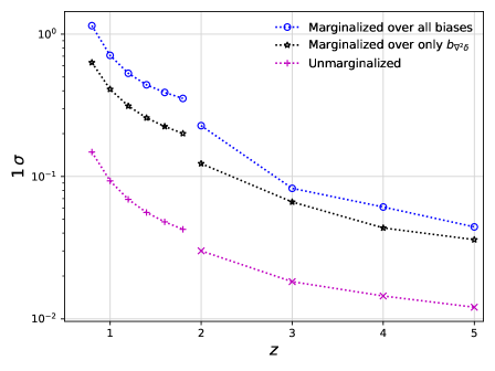
Figure 6: This figure is similar to that of Fig. 5 except only the combined power spectrum and bispectrum signal has been used and more importantly, the bias parameter marginalization has been turned on and off to understand the sensitivity of the signal to the bias parameters. As can be seen in the star marked curve, most of the marginalization induced signal degradation at high $z$ is coming from the marginalization over the Laplacian bias parameter $b_{\nabla^{2}\delta}$.

In Fig. 6, we illustrate the effects of marginalization over the bias parameters on the $\alpha$. There is about a factor of 10 (5) change in the sensitivity arising from the combination of five bias parameters ($b_{1},b_{2},b_{\mathcal{G}_{2}},b_{\nabla^{2}\delta},b_{\nabla^{2}\epsilon}$) that can affect the galaxy count similarly as a primordial isocurvature power spectral component in the case of Euclid (MM). Note that $b_{\nabla^{2}\delta}$ and $b_{\nabla^{2}\epsilon}$ parameters are multiplying higher power dependence in $k$ than others and thus lead to an approximate degeneracy of the high spectral power component coming from the isocurvature perturbations. Additionally due to the lack of $b_{\nabla^{2}\delta}$ and $b_{\nabla^{2}\epsilon}$ bias parameters in the tree-level bispectrum signal, the degeneracy from these biases, especially $b_{\nabla^{2}\delta}$, can become stronger than others. The degeneracy from $b_{\nabla^{2}\delta}$ is stronger than the degeneracy from $b_{\nabla^{2}\epsilon}$ because of its closer similarity of the associated $k$-dependent term with the isocurvature contribution for $n_{\rm{iso}}\sim 3.5$ (see Eq. (22) in contrast with Eq. (23) where $P_{\epsilon\epsilon}$ is a constant). This is highlighted in the star marked curve in Fig. 6 where we show the effect of marginalizing over only the Laplacian bias $b_{\nabla^{2}\delta}$. Higher loop computations as well as additional observables such as RSD will help reduce the degradation from the marginalization. The fact that Euclid shows a greater degradation from marginalization can be attributed to its lower redshift range which limits the $k$ range over which the signal is obtained due to the error envelope (e.g. a fixed $k$ value signal can be mimicked by almost any bias parametric degeneracy while a large $k$ range signal will not be reproducible exactly by the bias dependent spectral function). The decrease in degradation from the marginalization when accounting for a larger redshift range (see the marginalization over $b_{\nabla^{2}\delta}$ in Fig. 6) may be attributable to the redshift dependence of the biases, which is more constraining when probed over a larger range of redshifts.

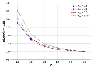
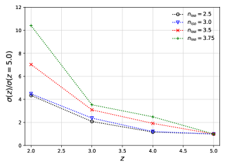
Figure 7: The dependence of the errors (Euclid on the left and MM on the right) on the isocurvature spectral index $n_{\mathrm{iso}}$ are shown. Only the power spectrum is used to make these plots since it is the dominant contribution to the sensitivities. Because MM is able to probe a larger number of high $k$ modes (due to the high redshift yielding more accurate theoretical computation), the spectral dependence is stronger for MM.

Fig. 7 illustrates the isocurvature spectral dependence of the sensitivities of Euclid and MM. Because MM observes a higher redshift universe where the perturbations have not grown as much, it has less theoretical error on large $k$ scales. This means that the degeneracies coming from the bias with high $k$ spectral dependence can vary more dramatically in the case of MM compared to Euclid, as seen in the figure. The decrease in the error with increasing $z$ seems to be continuing in the case of $n_{\mathrm{iso}}=3.75$ with MM, while for smaller spectral indices, there is an indication of saturation.

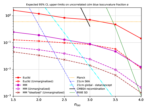
Figure 8: Our forecast for the Euclid and MM 2-sigma upper limits that can be placed on the isocurvature power spectral amplitude fraction $\alpha$ is shown as a function of the isocurvature spectral index. The results from Euclid and MM are drawn using “square” and “circular” markers respectively where solid (open) markers reflect marginalized (unmarginalized) errors. Because we are not including effects such as RSD or including higher loop computations, the actual upper limit should be somewhere between the unmarginalized and marginalized curves. For comparison, we also plot (without markers) some of the upper limits existing in a sample of the literature. The dotted (orange) line represents the current 2-sigma upper bound from Planck (Planck:2018jri, ). The solid thin (green) and thick (black) curves are obtained from (Chluba_2013, ) and (Lee:2021bmn, ) respectively. From previous forecasts based on 21cm line analyses, we plot thin (blue) and thick (cyan) dashdot curves obtained from (Sekiguchi:2013lma, ; Takeuchi:2013hza, ) and (Minoda:2021vyw, ) respectively.

In Fig. 8, we forecast the 95% confidence upper bound constraint on the uncorrelated CDM isocurvature fraction $\alpha$ for Euclid and MM. The fully marginalized Euclid errors for $\alpha$ are below the current Planck upper bound for $n_{\mathrm{iso}}\gtrsim 3$, and the fully marginalized MM errors are below the current Planck upper bound for $n_{\mathrm{iso}}\in[1.5,4]$. This result can be interpreted as the expected improvement achievable in the near future experiments. Because we have conservatively taken the linear bias from the “fiducial” categorization seen in Table 2 of (Ferraro:2019uce, ), the actual experimental sensitivity may be somewhat better than what we see in the solid curves with markers. Note that marginalized MM case is as good as unmarginalized Euclid case for the reasons described above.

Because we have not broken some parametric degeneracies using all available observables such as the RSD, to gain intuition on how much smaller the errors become with the degeneracy breaking, we also plot in Fig. 8 the unmarginalized case shown in dashed curves with markers. To understand the limitations imposed by the “fiducial” bias, we also plot (‘$\times$’ marked) the unmarginalized forecast for MM with the idealized linear biases and galaxy densities obtained from table 1 of (Ferraro:2019uce, ).

To give a sense of how the expected improvements compare with other future constraints, we sample results from the literature:

• In Planck:2018jri the authors analyzed the Planck data to constrain the isocurvature amplitude for various CDI models. For the uncorrelated ADI+CDI with free $n_{\rm{iso}}$ (axion-II) model they give the upper bound of $\alpha\lesssim 0.6$ at $k_{\rm{p}}=0.05$ Mpc^-1 over a range of spectral indices $1.55<n_{\rm{iso}}<3.67$. Since the Planck data is restricted to scales $k\lesssim 0.1$ Mpc^-1 where the isocurvature power hasn’t grown much, the data was not very constraining on the isocurvature spectral index and hence we consider a flat constraint over the range of indices considered in this work.

• Compared to the CMBS4 recombination forecast of (Lee:2021bmn, ) and PIXIE spectral distortion forecast (Chluba_2013, ), our results are obtained from much smaller $k$ values. For example, because (Lee:2021bmn, ) gave their results from 30 Mpc^-1, we extrapolated their results down to our $k$ range (with a pivot scale of $0.05$Mpc^-1) for comparison. There is a break in the black solid curve at $n_{\mathrm{iso}}=3$ because (Lee:2021bmn, ) has not given their results beyond that spectral index.

• (Sekiguchi:2013lma, ) gives a forecast on $\alpha$ from SKA based on 21cm emission from minihalos in the $z\in[5,20]$. Because the halo mass function used utilizes small virialized objects, these constraints are sensitive to nonlinear physics at $k\sim O(100)$Mpc^-1. Because $\alpha$ of (Sekiguchi:2013lma, ) is defined at the pivot scale of $k=0.002$Mpc^-1 and because their definition is the total isocurvature fraction while our $\alpha$ definition is the CDM isocurvature fraction, we have scaled their results appropriately in Fig. 8. The results of (Takeuchi:2013hza, ) are also similar. Note that if one uses the strongly nonlinear observables such as the number counts of virialized objects, then $n_{\mathrm{iso}}$ can be strongly constrained (Takeuchi:2013hza, ).

• In (Minoda:2021vyw, ), constraints are placed on the isocurvature fraction $\alpha$ coming from the shift in the 21cm absorption trough redshift which increases as $\alpha$ increases. In our plot, we give the bound coming from the assumption that Edges signal sees a trough starting at $z_{\mathrm{min}}=17.2$. Note that their equation 2.3 is inconsistent with its usage in equation 2.6 since with their 2.6, their equation 2.3 should have an extra factor of the square of CDM fraction and a factor of $1/3$ coming from the map of the primordial isocurvature perturbation to the matter power spectrum as discussed in Sec. II.

It is clear that near future experiments will realistically give at least an order of magnitude improvement in the constraint of the isocurvature amplitude for high spectral indices, even with the current theoretical computational technology of structure formation.

VIII Conclusion

We have presented a Fisher forecast of the Euclid and MegaMapper experimental sensitivities to primordial blue isocurvature spectrum of the uncorrelated CDM type. Our analysis utilized EFTofLSS (which uses SPT as part of its machinery) for the density field evolution because of its better UV control through N-body matched renormalization prescription and perturbative control of the uncertainties. This was then used with the bias expansion to obtain the theoretical prediction for galaxy number counts. We find that Euclid can give a factor of few improvement on the isocurvature spectral amplitude compared to the existing Planck constraints for $n_{\mathrm{iso}}\gtrsim 3$ while MM can give about 1 to 1.5 order of magnitude improvement for a broad range of $n_{\mathrm{iso}}$ (Fig. 8). MM tends to give a better constraint because of the larger signal data volume. Also, as expected, most of the signal is coming from the power spectrum and not the bispectrum for these experiments as can be seen in Fig. 5. Our forecast here represents conservative estimates, and an optimistic characterization (an $m_{UV}=24.5$ magnitude-limited dropout sample) of the experiments can improve the situation by an order of magnitude.

Going to higher redshift changes the isocurvature amplitude measurement sensitivities more significantly for higher spectral indices because of the larger amplitude that exists at larger $k$ values and higher redshift results in smaller error envelope for any given $k$ value. When comparing Euclid and MM, this effect is more significant for MM as can be seen in Fig. 7 because MM has a higher redshift reach. As can be seen in Fig. 6, the degradation in the constraint due to the bias marginalization is dominated by $b_{\nabla^{2}\delta}$ coming from the spectral similarities of this contribution when compared with an isocurvature spectrum of $n_{\mathrm{iso}}\sim 3.5$. This degeneracy does not seem to exist in scenarios without the large blue isocurvature contribution (DAmico:2019fhj, ).

One interesting theoretical feature of the isocurvature scenario in the EFTofLSS formalism is that the bare sound speed parameter $c^{2}$ is both cutoff dependent and may even become negative when the cutoff is taken above $\Lambda\gtrsim O(3)$ Mpc^-1 for sizable isocurvature amplitudes. Nonetheless, since physical observables are dependent only on the renormalized parameter $c_{{\rm ren}}^{2}$, we compare renormalized parameter $c_{{\rm ren}}^{2}$ for a sample of primordial spectra in Fig. 3. We see in the figure that the difference in the renormalized value of the effective sound speed squared $c_{{\rm ren}}^{2}$ between mixed and pure ICs at redshifts $z=0$ and $1$ obtained from the N-body simulations fits well a semi-analytic fitting formula for $\Delta c_{{\rm ren}}^{2}$ given in Appendix C which is applicable for values of $O(0.01)\lesssim\alpha<1$ and $2\leq n_{{\rm iso}}\leq 4$ for redshifts $z\leq 2$. Since the fluid parameter $c^{2}$ is degenerate with the higher order derivative bias $b_{\nabla^{2}\delta}$, a precise value of $c_{{\rm ren}}^{2}$ for mixed ICs is not required as we marginalize over the bias parameters. Hence, we found it adequate to work with the renormalized EFT or bias parameters of adiabatic ICs and apply them directly to the analysis/forecasts for mixed IC cosmologies.

Another peculiarity of the large blue spectral isocurvature scenario is the renormalization of various one-loop contributions to the galaxy power spectrum as discussed in Sec. V and the individual bare contributions given in Appendix B. Unlike the case for pure adiabatic ICs, the UV sensitivity for mixed ICs with large blue spectral indices is more severe since the one-loop terms $\mathcal{I}_{\delta^{(2)}\delta^{2}}(k)$, $\mathcal{I}_{\delta^{2}\delta^{2}}(k)$ and $\mathcal{I}_{\delta^{2}\mathcal{G}_{2}}(k)$ are UV divergent when $n_{{\rm iso}}\gtrsim 3.5$ and $\mathcal{F}_{\mathcal{G}_{2}}(k)$ is divergent when $n_{{\rm iso}}\gtrsim 3$. The set of terms $\mathcal{I}_{\delta^{(2)}\delta^{2}}(k)$, $\mathcal{I}_{\delta^{2}\delta^{2}}(k)$ and $\mathcal{I}_{\delta^{2}\mathcal{G}_{2}}(k)$ are renormalized by the higher order derivatives of stochastic terms in the bias expansion, and similarly the leading divergent piece from $\mathcal{F}_{\mathcal{G}_{2}}(k)$ is renormalized by redefining the $b_{\nabla^{2}\delta}$ bias parameter of the leading higher-derivative operator. The renormalized one-loop contributions are given in Eq. set (31).

Fisher forecasts have well known limitations. For example, the assumption of a Gaussian likelihood for the Fisher analysis may break down at scales comparable or much smaller than nonlinear scales due to loop corrections as well as one-halo and higher order perturbative terms. Similarly, we have also neglected the small correlations among the redshift bins for each of the surveys. Additionally the parameter degeneracies in a Fisher analyses can be misleading since they are only considered at leading order by construction (Ryan:2022qpa, ). Beyond the limitations coming from the Fisher formalism, there are limitations in the bias functions used here. In this work, we have used the fiducial values for higher order Laplacian biases $b_{\nabla^{2}\delta}$ and $b_{\nabla^{2}\epsilon}$ from the literature wherein the ICs were taken to be purely adiabatic because for small isocurvature amplitudes $\alpha\sim O(0.01)$, we do not expect the renormalized biases to be very different from those of the adiabatic case, and marginalization seems to remove dependences upon the exact fiducial values of the biases. In summary we do not expect any of these limitations to strongly affect our forecast.

There are many interesting future directions related to this work. The most immediate extension of our work will be to include RSDs. RSD effects can break some of the bias degeneracies significantly since these include velocity fields such that each multipole provides an additional observable, wherein the biases have varying sensitivities to these multipoles. For example, Chudaykin:2019ock showed that RSD significantly improves constraints on neutrino masses, and we expect that a similar improvement is possible in the case of blue isocurvature perturbations.

One important theoretical caveat to the scenario that we are considering is that the primordial isocurvature spectrum is assumed to rise indefinitely without a cutoff. In reality, one can show (Chung:2015tha, ) that when the spectral index is larger than about 2.4, the energy density in the dark matter gets diluted away by the inflationary expansion. Hence, a more realistic spectrum should have a cutoff and become flat as in the model of (Kasuya:2009up, ). This can lead to a break in the degeneracy with the bias parameters. Furthermore, as shown in (Chung:2021lfg, ), when the underlying dynamics that generates the blue spectrum is underdamped, a large (an amplitude multiplicative enhancement of $O(30)$) oscillatory features can arise in the primordial isocurvature power spectrum. Such an oscillatory spectrum will also tend to break the parametric degeneracies differently than the case of the power law primordial spectrum considered in the present work. A future work dedicated to the study of these scenarios would be useful.

It would be interesting to include massive neutrinos in the theoretical prediction to see how much the neutrino mass constraints degrade due to the presence of blue CDM isocurvature component which can qualitatively compensate for the power erasure due to the neutrino free streaming. Although naively we do not expect a quantitatively precise degeneracy between $\alpha$ and neutrino masses since neutrino suppression is roughly constant at small scales unlike scale-dependent blue isocurvature signals, a low-$n_{{\rm iso}}$ isocurvature signal can cancel some suppression from a massive neutrino at quasi non-linear scales.

Another natural target of exploration is to go beyond one-loop power spectrum and tree-level bispectrum to explore possible trade-offs between larger number of available modes and proliferation of bias parameters. Previous analyses from the literature (Eggemeier_2019, ; Philcox:2022frc, ) suggest that the expected improvement is paltry due to the marginalization over an extended set of biases unless strong priors can be placed on the bias parameters. Stronger priors on the values and covariance of bias parameters could in principle be obtained from simulations, if these simulations can bracket the range of physically plausible small-scale physics. A different strategy to break parameter degeneracies is to perform a field level analysis rather than to calculate N-point correlation functions. That field level analysis can break bias parameter degeneracies was recently shown in Baumann:2021ykm for the case of primordial non-Gaussianities. Yet another possible alternative is to come up with a non-perturbative description of tracers in the case of mixed initial condition/high spectral index situations which is unlikely to have the same degeneracy as the perturbative expansion. For example, blue isocurvature can strongly affect the halo mass function. We hope to explore some of these directions in the future.

In addition, we observe from Fig. 4 that for the low redshift surveys with large number densities, the signal is primarily limited by the theoretical error. In Fig. 2 we noted that the two-loop error envelope in Eq. (27) is somewhat conservative and seems to be overestimating the actual error between the one-loop EFT and the N-body data. Consequently, obtaining a more accurate estimation of the theory error specifically for the biased tracers could potentially result in improved forecast and fitting outcomes in future analyses.

Finally, since our Eq. (78) was derived for $z\lesssim 2$, it would useful to more accurately compute $\Delta c_{\mathrm{ren}}^{2}$ for higher redshifts (for example in the range $2<z<10$) if there are more observables to break its degeneracy with the biases. The current fitting function from N-body data suggests that the ratio of $\Delta c_{{\rm ren}}^{2}/c_{{\rm ren,AD}}^{2}\propto D_{+}^{1.2}(z)$ increases almost linearly with redshift. This can be explained if we consider that the renormalized parameter $c_{{\rm ren}}^{2}$ inherits UV effects due to the non-linear clustering at small scales. The non-linear scale $k_{{\rm NL}}$ increases with redshift $z$, and hence the difference in the linear power spectra $P_{11}^{{\rm MX}}(k)-P_{11}^{{\rm AD}}(k)$ at $k=k_{{\rm NL}}$ also increases for $n_{{\rm iso}}>n_{{\rm ad}}$. Consequently, we expect a larger power from mixed ICs at small scales which may explain why the ratio $\Delta c_{{\rm ren}}^{2}/c_{{\rm ren,AD}}^{2}$ increases with redshift $z$. On the other hand, given that the bare $c^{2}$ can become negative for $\Lambda\gtrsim O(3)$, there is an unclear interpretation of this parameter, which leaves room for more intricate UV dynamics being at play here for the isocurvature scenario. A nonlinear UV model exploration of this issue may be useful to further elucidate the differences in $c_{{\rm ren,MX}}^{2}$ and $c_{{\rm ren,AD}}^{2}$.

Appendix A Renormalization scheme

In a perturbatively expanded effective field theory valid in the IR and coarse grained over a UV inverse length scale $\Lambda$, one writes down all possible terms consistent with the symmetries up to a given perturbative order of computation and adjusts the coefficients of the terms using a chosen prescription called a renormalization scheme. In this section, we list the renormalization scheme used for the EFTofLSS and the bias expansion for this paper.

Let there be a set of (composite) operators $\{\mathcal{O}_{i}\}$ that can mix because they share the symmetry representation of the theory. Note that $\mathcal{O}_{i}$ can involve gravitational potentials which in the density fields can be nonlocal. In the EFTofLSS, some of the $\mathcal{O}_{i}$ are defined using expressions obtained from a derivative expansion. Define the renormalized operator $\left[\mathcal{O}_{i}\right]$ as (Assassi:2014fva, )

$$\left[\mathcal{O}_{i}\right]=\mathcal{O}_{i}+\sum_{j}Z_{ij}(\Lambda)\mathcal{O}_{j},$$ (51)

where $Z_{ij}$ contain the counterterm coefficients appropriately chosen to make the correlators involving $\left[\mathcal{O}_{i}\right]$ independent of $\Lambda$. To determine $Z_{ij}(\Lambda)$, (Assassi:2014fva, ) proposes a natural sufficient condition that all $n$-point correlation functions be finite in the large-scale limit $(k\rightarrow 0)$. This is equivalent to the following renormalization prescription for the composite operators $\mathcal{O}_{i}$:

$$\left\langle[O_{i}](\vec{k})\delta^{(1)}(\vec{k}_{1})\cdots\delta^{(1)}(\vec{k}_{n})\right\rangle=\left\langle O_{i}(\vec{k})\delta^{(1)}(\vec{k}_{1})\cdots\delta^{(1)}(\vec{k}_{n})\right\rangle_{{\rm tree}}\qquad\forall k_{i}\rightarrow 0$$ (52)

where $\delta^{(1)}(k)$ is the linear matter over-density. This implies for Eq. (51) the condition that the loop contributions cancel since

$$\left\langle O_{i}(\vec{k})\delta^{(1)}(\vec{k}_{1})\cdots\delta^{(1)}(\vec{k}_{n})\right\rangle_{{\rm loop}}=-\sum_{j}Z_{ij}\left\langle O_{j}(\vec{k})\delta^{(1)}(\vec{k}_{1})\cdots\delta^{(1)}(\vec{k}_{n})\right\rangle\qquad\forall k_{i}\rightarrow 0$$ (53)

where the subscript “loop” refers to the diagrams that involve at least one contraction between the internal legs of the operator $O_{i}$, whereas the “tree” diagrams in Eq. (52) do not contain such contractions. Since the operator set has a finite number of elements at any given perturbative order, the dimensionality of $Z_{ij}(\Lambda)$ is finite in perturbation theory at a given truncation order. This means that the number of conditions that needs to be imposed in the form Eq. (52) to determine $Z_{ij}(\Lambda)$ is finite.

In the case of describing coarse grained fluid density fields, the $n$th order perturbation theory operators are partly those of SPT which form one susbset of composite operators: e.g. $\delta(k)=\delta^{(1)}(k)+\delta^{(2)}(k)+...$ with $\delta^{(2)}(k)=\int d^{3}q_{1}d^{3}q_{2}F_{2}(q_{1},q_{2})\delta^{(1)}(q_{1})\delta^{(1)}(q_{2})$. Other composite operator terms of $\delta(k)$ in EFTofLSS include a derivative expansion of the effective pressure term

$$\delta^{(c_{1})}(k,z)\approx c^{2}(\Lambda,z)k^{2}\delta^{(1)}(k,z)$$ (54)

where $c^{2}(\Lambda,z)$ is an effective cutoff-dependent sound speed squared parameter. The function $c^{2}(\Lambda,z)$ is fixed by a couple of conditions that deviate from the condition of Eq. (53). We write

$$c^{2}(\Lambda,z)=c_{\Lambda}^{2}(k_{\rm{ren}},\Lambda,z)+c_{\rm{ren}}^{2}(k_{\rm{ren}},z)$$ (55)

where $k_{\rm ren}$ should not be viewed as a renormalization scale but as a parameter defining the subtraction scheme. The function $c_{\Lambda}^{2}(k_{\rm{ren}},\Lambda,z)$ is fixed by the choice

$$c_{\Lambda}^{2}(k_{\rm{ren}},\Lambda,z)=\frac{P_{13}(k_{{\rm ren}},\Lambda,z)}{2k_{{\rm ren}}^{2}P_{{\rm 11}}(k_{{\rm ren}},z)}$$ (56)

with $k_{\rm{ren}}\sim 0.1h$ Mpc^-1 in this work. The function $c_{\rm{ren}}^{2}(k_{\rm{ren}},z)$ is obtained by a best-fit to the numerical simulations data. This in the language of ordinary quantum field theory (QFT) renormalization procedure corresponds indirectly to a judicious choice of the renormalization scale that minimizes the theory error. Because $k_{\rm ren}$ here corresponds to a definition of a subtraction scheme, the analog of the renormalization scale $\mu$ in QFT does not explicitly appear in Eq. (55).

The bias expansion for galaxies is also a composite operator expansion. In the notation of (Desjacques_2018, )

$$\delta_{g}(\vec{x})=b_{\epsilon}[\epsilon(\vec{x})]+\sum_{\mathcal{O}}\left\{b_{\mathcal{O}}+[\epsilon_{\mathcal{O}}(\vec{x})]\right\}[\mathcal{O}(\vec{x})].$$ (57)

where $\epsilon_{\mathcal{O}}(\vec{x})$ are the stochastic fields which really represent a class of short distance effects and $b_{\mathcal{O}}$ are coefficients that can absorb divergences based on the chosen renormalization scheme. The bias parameters also contain cutoff dependences that can be adjusted according to Eq. (52) to make the observed $\delta_{g}$ correlators $\Lambda$-independent.

Appendix B Galaxy one-loop contributions

The one-loop contribution to the galaxy two-point correlation function in $k$-space is given by the following convolutional loop integral terms taken from (Assassi:2014fva, ):

$$\mathcal{I}_{\delta^{(2)}\delta^{2}}(k,z) =2\int_{q}F_{2}\left(\vec{q},\vec{k}-\vec{q}\right)P_{{\rm 11}}(q,z)P_{{\rm 11}}(|\vec{k}-\vec{q}|,z),$$ (58)

$$\mathcal{I}_{\delta^{(2)}\mathcal{G}_{2}}(k,z) =2\int_{q}\sigma^{2}\left(\vec{q},\vec{k}-\vec{q}\right)F_{2}\left(\vec{q},\vec{k}-\vec{q}\right)P_{{\rm 11}}(q,z)P_{{\rm 11}}(|\vec{k}-\vec{q}|,z),$$ (59)

$$\mathcal{F}_{\mathcal{G}_{2}}(k,z) =4P_{{\rm 11}}(k,z)\int_{q}\sigma^{2}\left(\vec{q},\vec{k}-\vec{q}\right)F_{2}\left(\vec{k},-\vec{q}\right)P_{{\rm 11}}(q,z),$$ (60)

$$\mathcal{I}_{\delta^{2}\delta^{2}}(k,z) =2\int_{q}P_{{\rm 11}}(q,z)P_{{\rm 11}}(|\vec{k}-\vec{q}|,z),$$ (61)

$$\mathcal{I}_{\mathcal{G}_{2}\mathcal{G}_{2}}(k,z) =2\int_{q}\left(\sigma^{2}\left(\vec{q},\vec{k}-\vec{q}\right)\right)^{2}P_{{\rm 11}}(q,z)P_{{\rm 11}}(|\vec{k}-\vec{q}|,z),$$ (62)

$$\mathcal{I}_{\delta^{2}\mathcal{G}_{2}}(k,z) =2\int_{q}\sigma^{2}\left(\vec{q},\vec{k}-\vec{q}\right)P_{{\rm 11}}(q,z)P_{{\rm 11}}(|\vec{k}-\vec{q}|,z),$$ (63)

where $\int_{q}\equiv\int\frac{d^{3}q}{\left(2\pi\right)^{3}}$, $\sigma^{2}(\vec{k}_{1},\vec{k}_{2})=\left(\vec{k}_{1}\cdot\vec{k}_{2}/k_{1}k_{2}\right)^{2}-1$, and $F_{2}$ is the mode-coupling kernel for $\delta_{k}^{(2)}$.

Appendix C Semi-analytic expression for $c_{{\rm ren,MX}}^{2}$

Consider the one-loop matter power spectrum in the EFTofLSS perturbation theory from Eq. (12),

$$P_{{\rm 1-EFT}}(k,z) =D^{2}(z)P_{11}(k)+D^{4}(z)\left[P_{{\rm 22}}(k)+P_{{\rm 13}}(k,\Lambda)-2D^{-2}(z)c_{{\rm\Lambda}}^{2}(k_{{\rm ren}},\Lambda,z)k^{2}P_{11}(k)\right]$$

$$-2D^{2}(z)c_{{\rm ren}}^{2}(k_{{\rm ren}},z)k^{2}P_{11}(k).$$ (64)

where $D(z)$ is the normalized growth function, $D(z)\equiv D_{+}(z)/D_{+}(0)$. We restrict the above expression to scales where the two-loop and other higher order contributions are negligible such that $P_{{\rm 1-EFT}}(k)\approx P_{{\rm NL}}(k)$ where $P_{{\rm NL}}(k)$ is the exact non-linear power spectrum. We consider a renormalization choice where the $\Lambda$-dependent counterterm parameters $c_{\Lambda}^{2}(k_{{\rm ren}},\Lambda,z)$ in Eq. (64) is expressed as:

$$c_{{\rm\Lambda}}^{2}(k_{{\rm ren}},\Lambda,z) =\frac{P_{13}(k_{{\rm ren}},\Lambda,z)}{2k_{{\rm ren}}^{2}P_{{\rm 11}}(k_{{\rm ren}},z)}=D^{2}(z)\frac{P_{13}(k_{{\rm ren}},\Lambda)}{2k_{{\rm ren}}^{2}P_{{\rm 11}}(k_{{\rm ren}})}.$$ (65)

At the scale $k=k_{{\rm ren}}$, the expression in Eq. (64) reduces to

$$P_{{\rm 1-EFT}}(k_{{\rm ren}},z)=D^{2}(z)P_{11}(k_{{\rm ren}})+D^{4}(z)P_{{\rm 22}}(k_{{\rm ren}})-2D^{2}(z)c_{{\rm ren}}^{2}(k_{{\rm ren}},z)k_{{\rm ren}}^{2}P_{11}(k_{{\rm ren}}).$$ (66)

Next we take the difference in the one-loop matter power spectra for the two different sets of initial conditions: namely, pure adiabatic (AD), and mixed adiabatic and isocurvature (MX) at $k=k_{{\rm ren}}$ written as

$$P_{{\rm 1-EFT}}^{{\rm MX}}(k_{{\rm ren}},z)-P_{{\rm 1-EFT}}^{{\rm AD}}(k_{{\rm ren}},z) =D^{2}(z)\left(P_{11}^{{\rm MX}}(k_{{\rm ren}})-P_{11}^{{\rm AD}}(k_{{\rm ren}})\right)$$

$$+D^{4}(z)\left(P_{22}^{{\rm MX}}(k_{{\rm ren}})-P_{22}^{{\rm AD}}(k_{{\rm ren}})\right)$$

$$-2D^{2}(z)k_{{\rm ren}}^{2}\left(c_{{\rm ren,MX}}^{2}(k_{{\rm ren}},z)P_{11}^{{\rm MX}}(k_{{\rm ren}})-c_{{\rm ren,AD}}^{2}(k_{{\rm ren}},z)P_{11}^{{\rm AD}}(k_{{\rm ren}})\right).$$ (67)

In the above expression, the change in the nonlinear matter power spectrum due to the variation in $c_{{\rm ren}}^{2}$ can be written as

$$\Delta P_{{\rm NL,c}}(k,z)=-2k_{{\rm ren}}^{2}\Delta c_{{\rm ren}}^{2}(k_{{\rm ren}},z)P_{11}^{{\rm MX}}(k_{{\rm ren}},z)$$ (68)

where

$$\Delta c_{{\rm ren}}^{2}(k_{{\rm ren}},z) =c_{{\rm ren,MX}}^{2}(k_{{\rm ren}},z)-c_{{\rm ren,AD}}^{2}(k_{{\rm ren}},z).$$ (69)

Since the parameter $c_{{\rm ren}}^{2}$ is a leading order residual contribution after integrating out the UV scales, its variation due to the additional isocurvature power is a nontrivial contribution from the nonlinear-nonperturbative modes.

By defining the relative fractional difference for a power spectrum contribution $P_{i}$ as

$$g_{i}(k,z)=\frac{P_{i}^{{\rm MX}}(k,z)-P_{i}^{{\rm AD}}(k,z)}{P_{i}^{{\rm AD}}(k,z)},$$ (70)

we can write LHS in Eq. (68) as

$$\Delta P_{{\rm NL,c}}(k,z)=g_{{\rm NL,c}}(k,z)P_{{\rm NL}}^{{\rm AD}}(k,z)$$ (71)

where we take $P_{{\rm NL}}^{{\rm AD}}\approx P_{{\rm 1-EFT}}^{{\rm AD}}$. Substituting Eq. (71) in Eq. (68), we obtain

$$\Delta P_{{\rm{\rm NL,c}}}(k_{{\rm ren}},z)\equiv g_{{\rm NL,c}}(k_{{\rm ren}},z)P_{{\rm NL}}^{{\rm AD}}(k_{{\rm ren}},z)=\left(1+g_{{\rm 11}}(k_{{\rm ren}})\right)\frac{\Delta c_{{\rm ren}}^{2}(k_{{\rm ren}},z)}{c_{{\rm ren,AD}}^{2}(k_{{\rm ren}},z)}P_{c}^{{\rm AD}}(k_{{\rm ren}},z)$$ (72)

where $g_{11}(k,z)\equiv g_{11}(k)=\Delta P_{11}(k)/P_{11}^{{\rm AD}}(k)$ is obtained from Eq. (3) as

$$g_{11}(k)=\alpha\left(\frac{f_{c}}{3}\right)^{2}\left(\frac{T_{{\rm iso}}(k)}{T_{{\rm ad}}(k)}\right)^{2}\left(\frac{k}{k_{\mathrm{p}}}\right)^{n_{{\rm iso}}-n_{{\rm ad}}}.$$ (73)

By factorizing $g_{{\rm NL,c}}(k_{{\rm ren}},z)$ as

$$g_{{\rm NL,c}}(k_{{\rm ren}},z)=-2k_{{\rm ren}}^{2}\,g_{{\rm 11}}(k_{{\rm ren}}){\rm B}(k_{{\rm ren}},n_{{\rm iso}},\alpha,z)$$ (74)

where the ${\rm B}$ term can either be positive or negative depending upon the non-linear corrections, we arrive at the expression

$$\Delta c_{{\rm ren}}^{2}(k_{{\rm ren}},z)\approx\frac{P_{{\rm NL}}^{{\rm AD}}(k_{{\rm ren}},z)}{P_{11}^{{\rm AD}}(k_{{\rm ren}},z)}\times\frac{g_{{\rm 11}}(k_{{\rm ren}})}{1+g_{{\rm 11}}(k_{{\rm ren}})}\times{\rm B}(k_{{\rm ren}},n_{{\rm iso}},\alpha,z).$$ (75)

In the above expression, we note that the first prefactor is isocurvature independent and is completely determined from the adiabatic component by replacing $P_{{\rm NL}}^{{\rm AD}}(k_{{\rm ren}},z)$ with $P_{{\rm 1-EFT}}^{{\rm AD}}(k_{{\rm ren}},z)$ and using an empirically measured value of the renormalized fluid parameter $c_{{\rm ren,AD}}^{2}(k_{{\rm ren}},z)$ from N-body simulations or data. The second term is analytically computable for a given fiducial choice of isocurvature model parameters $n_{{\rm iso}}$ and $\alpha$ and measures the fraction of linear power carried by the isocurvature modes. The ${\rm B}$ term captures the difference in the power for the density fluctuations between the mixed isocurvature (MX) and pure adiabatic (AD) from backreaction of nonperturbative UV modes on large scales and can be obtained by fitting to the numerical results from N-body simulations. Hence, $B\neq 0$ is an indirect measure of the relative difference in the nonlinear corrections from the small scales to the coarse-grained effective fluid due to the additional contribution from primordial blue isocurvature fluctuations.

In order to complete our estimation of $c_{{\rm ren,MX}}^{2}(k_{{\rm ren}},z)$, we give the following empirical fitting function for ${\rm B}$ at $k_{{\rm ren}}=0.1{\rm h/Mpc}$ by matching with the data from N-body simulations:

$${\rm B}(k_{{\rm ren}}=0.1{\rm h/Mpc},n_{{\rm iso}},\alpha,z) =0.272\times D(z)^{0.858}\alpha^{-0.147}\left(n_{{\rm iso}}-n_{{\rm ad}}\right)\left(\frac{k_{s}}{k_{{\rm p}}}\right)^{n_{{\rm iso}}-n_{{\rm ad}}}$$ (76)

where

$$k_{s}\approx 0.2174\,{\rm Mpc^{-1}}$$ (77)

represents a fixed scale.

Substituting the above empirical expression into Eq. (75) we obtain the result

$$\Delta c_{{\rm ren}}^{2}(k_{{\rm ren}}=0.1{\rm h/Mpc},z) \approx\frac{P_{{\rm 1-EFT}}^{{\rm AD}}(k_{{\rm ren}},z)}{P_{11}^{{\rm AD}}(k_{{\rm ren}},z)}\times\frac{g_{{\rm 11}}(k_{{\rm ren}})}{1+g_{{\rm 11}}(k_{{\rm ren}})}\times$$

$$\left(0.272\,D(z)^{0.858}\alpha^{-0.147}\left(n_{{\rm iso}}-n_{{\rm ad}}\right)\left(\frac{k_{s}}{k_{{\rm p}}}\right)^{n_{{\rm iso}}-n_{{\rm ad}}}\right)$$ (78)

for the estimation of renormalized fluid parameter $c_{{\rm ren,MX}}^{2}=c_{{\rm ren,AD}}^{2}+\Delta c_{{\rm ren}}^{2}$ for mixed isocurvature initial conditions for fiducial values of $O(0.01)\lesssim\alpha<1$ and $2\leq n_{{\rm iso}}\leq 4$ for redshift range $z\leq 2$. The value of $\Delta c_{{\rm ren}}^{2}$ at a different renormalization scale can be obtained from the following expression:

$$\Delta c_{{\rm ren}}^{2}(k_{{\rm ren,1}},z) =\Delta c_{{\rm ren}}^{2}(k_{{\rm ren}},z)+\left(\Delta c_{{\rm\Lambda}}^{2}(k_{{\rm ren}},\Lambda,z)-\Delta c_{{\rm\Lambda}}^{2}(k_{{\rm ren,1}},\Lambda,z)\right)$$ (79)

where $k_{{\rm ren}}$ and $k_{{\rm ren,1}}$ are the old and new renormalization scales respectively, and $\Delta c_{{\rm\Lambda}}^{2}(k_{{\rm ren}},\Lambda,z)\equiv c_{{\rm\Lambda,MX}}^{2}(k_{{\rm ren}},\Lambda,z)-c_{{\rm\Lambda,AD}}^{2}(k_{{\rm ren}},\Lambda,z)$ is the difference in the square of the $\Lambda$-dependent counterterm parameters as defined in Eq. (65).

Appendix D Fisher matrix and theoretical error covariance

For the purpose of Fisher forecasting, we consider a Gaussian likelihood function (dodelson2020modern, ):

$$\mathcal{L}=\frac{1}{\sqrt{\left(2\pi\right)^{N_{c}}|C|}}\exp\left[-\frac{1}{2}\left(d-t\right)^{{\rm T}}C^{-1}\left(d-t\right)\right]$$ (80)

where $N_{c}$ is the total number of momentum configurations (for the power spectrum (bispectrum), $N_{c}$, is the total number of momentum bins (triangle configurations)). Here, $d$ and $t$ are the data and theoretical prediction vectors while $C$ is the covariance matrix which is to be taken as the sum of data covariance and the theoretical covariance (Baldauf:2016sjb, ; dodelson2020modern, ). Using the likelihood function, the Fisher information matrix is defined as the curvature of the likelihood at the fiducial parameter set along each model parameter $p_{n}$:

$$F_{ij}=-\left.\left\langle\frac{\partial^{2}\ln\mathcal{L}}{\partial p_{i}\partial p_{j}}\right\rangle\right|_{p=p_{{\rm fid}}},$$ (81)

where the matrix is evaluated at a fiducial point in parameter space $p_{{\rm fid}}$ and $\left\langle...\right\rangle$ implies taking an ensemble average. The Fisher matrix then allows one to understand how well various parameters of the theoretical model can be constrained. The unmarginalized error on one single parameter $p_{i}$ is estimated by the inverse of the respective diagonal element in the Fisher matrix

$$\sigma(p_{i})=\frac{1}{\sqrt{F_{ii}}}.$$ (82)

On the other hand, one can obtain marginalized error estimate by integrating the probability over all other model parameters. This is easily obtained from the Fisher information matrix as

$$\sigma(p_{i})=\sqrt{\left(F^{-1}\right)_{ii}}.$$ (83)

For marginalization over a smaller set of parameters, we refer the reader to (Coe:2009xf, ). From the definitions given in Eqs. (80) and (81) it follows that the power spectrum Fisher matrix is (dodelson2020modern, ):

$$F_{ij}^{s}=\sum_{z_{l}}\sum_{k,k^{\prime}}\frac{\partial P_{s}\left(k,z_{l}\right)}{\partial p_{i}}\left(C^{-1}(z_{l})\right)_{kk^{\prime}}^{s}\frac{\partial P_{s}\left(k^{\prime},z_{l}\right)}{\partial p_{j}}$$ (84)

where the sum runs over all measured binned redshifts and momentum bins and $P_{s}$ is the theoretical power spectrum where $s$ characterizes the spectrum type which we can be either matter or biased tracer like galaxy, halo or mixed matter-galaxy. All terms are evaluated at the fiducial values of the model parameters. Here we will consider that the redshift bins are wide enough such that the cross spectra between the bins vanish (see discussion in (LESGOURGUES_2006, ) and Chapter 14 of (dodelson2020modern, ) for details). Also see (Bellomo:2020pnw, ) for the situations where these assumptions might fail.

The power spectrum covariance matrix $C_{kk^{\prime}}^{s}$ can be written as sum of data covariance ($C_{d,kk^{\prime}}^{s}(z_{l})$) and theory error estimate covariance ($C_{e,kk^{\prime}}^{s}(z_{l})$) (Baldauf:2016sjb, ):

$$C_{kk^{\prime}}^{s}(z_{l})=C_{d,kk^{\prime}}^{s}(z_{l})+C_{e,kk^{\prime}}^{s}(z_{l}).$$ (85)

The data covariance for the galaxy power spectrum is

$$C_{d,kk^{\prime}}^{s}(z_{l})=\frac{\left(2\pi\right)^{3}}{V(z_{l})}\frac{f_{{\rm sky}}^{-1}}{2\pi k^{2}k_{{\rm bin}}}\left(P_{s}(k,z_{l})+P_{s,{\rm shot}}(z_{l})\right)^{2}\delta_{kk^{\prime}}$$ (86)

where $V(z_{l})$ is the volume of the shell centered at $z_{l}$ with the bin width $\Delta z_{l}$ and is given by the expression

$$V(z_{l})=\frac{4\pi}{3}\left[r^{3}\left(z_{l}+\frac{\Delta z}{2}\right)-r^{3}\left(z_{l}-\frac{\Delta z}{2}\right)\right],$$ (87)

$r(z^{\prime})$ is the comoving distance to the redshift $z^{\prime}$, $f_{{\rm sky}}$ is the observed fraction of sky, $k_{{\rm bin}}$ is the momentum bin-width and $P_{{\rm shot}}$ is the contribution from the shot-noise which is equal to $1/\bar{n}(z_{l})$ in case of galaxies where $\bar{n}$ is the average number density of galaxies. The theoretical error covariance matrix as defined in (Baldauf:2016sjb, ) is given as

$$C_{e,kk^{\prime}}^{s}(z_{l})=E_{k}^{s}\exp\left[-\frac{\left(k-k^{\prime}\right)^{2}}{2\Delta k^{2}}\right]E_{k^{\prime}}^{s}$$ (88)

where $E_{k}^{s}\equiv E^{s}(k,z)$ is the theoretical error estimate (smoothed envelope without any fast variation as a function of wave vectors) for the spectrum type $s$. The explicit expressions for $E^{s}(k,z)$ are given in Sec. VI.2. Note that in the above expression for $C_{e}^{s}$, the errors in various momentum bins are correlated through a Gaussian correlation with a common width set by $\Delta k$. In our analysis we found that a choice of $0.05<\Delta k\left({\rm h/Mpc}\right)^{-1}<0.13$ does not lead to significant changes $(\lesssim 10\%)$ in the error estimates from Fisher analysis. For a more detailed discussion refer to (Baldauf:2016sjb, ; Chudaykin:2019ock, ). Similarly, for bispectrum, the Fisher information matrix is given as

$$F_{ij}^{b}=\sum_{z_{l}}\sum_{T,T^{\prime}}\frac{\partial B_{s}\left(T,z_{l}\right)}{\partial p_{i}}\left(C^{-1}(z_{l})\right)_{TT^{\prime}}^{s}\frac{\partial B_{s}\left(T^{\prime},z_{l}\right)}{\partial p_{j}}$$ (89)

where the sum runs over all possible triangle configurations such that $\vec{k}_{1}+\vec{k}_{2}+\vec{k}_{3}=0$ with the following ordering of the scales $k_{1}\geq k_{2}\geq k_{3}$. Thus,

$$\sum_{T}\equiv\sum_{k_{1}=k_{\min}}^{k_{\max}}\sum_{k_{2}=k_{\min}}^{k_{1}}\sum_{k_{3}=k_{*}}^{k_{2}}$$ (90)

where $k_{*}=\max\left(k_{\min},k_{1}-k_{2}\right)$. The total bispectrum covariance matrix is given as

$$C_{TT^{\prime}}^{s}(z_{l})=\delta_{TT^{\prime}}\frac{\left(2\pi\right)^{3}}{V(z_{l})}s_{123}\frac{\pi f_{{\rm sky}}^{-1}}{k_{{\rm bin}}^{3}}\frac{1}{k_{1}k_{2}k_{3}}\prod_{j=1}^{3}\left(P_{s}(k_{j},z_{l})+P_{s,{\rm shot}}(z_{l})\right)+\left(C_{e}^{s}(z_{l})\right)_{TT^{\prime}}$$ (91)

where $s_{123}$ is the symmetry factor equal to $1,2$ or $6$ for general, isosceles, and equilateral triangles respectively.

While the data covariance falls as $1/k^{2}$ for small scales, the theory error covariance tends to increase rapidly as we approach scale, $k_{{\rm Th}}(z)$, where the underlying theory tends to break down. Hence, the signal to noise ratio is maximum close to the minimum of the sum of the two covariances. Therefore, by including theoretical error within the covariance matrix the signal is naturally cutoff at scales $\approx k_{{\rm Th}}(z)$.

Combining the power spectrum and bispectrum information is equivalent to summing up the Fisher matrices

$$F=F_{p}+F_{b}+{\rm diag\left(1/\sigma_{p_{i}}^{2}\right)}$$ (92)

where $\sigma_{p_{i}}$ is the assumed prior on a parameter $p_{i}$.

Appendix E Comparison to Halofit

Some forecasts use theoretical predictions for non-linear galaxy clustering generated with Halofit (Takahashi:2012em, ). However, it was shown in (Reimberg:2018kwn, ) that because the Halofit is not sufficiently accurate in reproducing the derivatives of the power spectrum, other methods should be used for Fisher forecasts. Furthermore, as can be seen in Fig. 9, if we apply Halofit naively without adjusting its coefficients to isocurvature (by fitting them to simulations with isocurvature), it grossly under-predicts the power on BAO scales for a mixed state containing a sizable fraction of blue isocurvature power, as we now explain. Halofit relies on the Halo model Takahashi:2012em for its fitting form, and the mismatch between the fit and the data appears in the two-halo term which governs the large-scale behavior. This may be explained if we note that the two-halo term in Halofit is evaluated using a set of fitting parameters, ($\alpha_{n},\,\beta_{n}$), that are given by polynomials as a function of the effective spectral index $n_{\rm{eff}}$ and the curvature $C$ of the linear variance $\sigma^{2}(R)$ evaluated at the scale $k_{\sigma}$ where the $\sigma^{2}(1/k_{\sigma})=1$: the two-halo term contribution to the power spectrum is

$$\Delta_{Q}^{2}(k)=\Delta_{L}^{2}(k)\frac{\left(1+\Delta_{L}^{2}(k)\right)^{\beta_{n}}}{1+\alpha_{n}\Delta_{L}^{2}(k)}e^{-f(k/k_{\sigma})}$$ (93)

where $\Delta_{L}^{2}$ is the dimensionless linear power spectrum, $f(y)=y/4+y^{2}/8$, and

$$\alpha_{n} = \left|6.0835+1.3373n_{\mathrm{eff}}-0.1959n_{\mathrm{eff}}^{2}-5.5274C\right|$$ (94)

$$\beta_{n} = 2.0379-0.7354n_{\mathrm{eff}}+0.3157n_{\mathrm{eff}}^{2}+1.2490n_{\mathrm{eff}}^{3}+0.3980n_{\mathrm{eff}}^{4}-0.1682C$$ (95)

The coefficients such as 5.5274 of Eq. 94 of the polynomial functions were obtained by fitting the halo model to a large set of $\Lambda$CDM simulations without any blue isocurvature amplitude. Hence, it may be argued that the fitting coefficients are not well suited to give an accurate prediction for the non-linear power spectrum with a sizable isocurvature fraction. To illustrate the difference, we found that the value of the parameter set $\left(n_{\rm{eff}},\,C\right)$ for the pure adiabatic and our fiducial mixed scenario (with $n_{\rm{iso}}=3.75$ and $\alpha=0.25$) at redshift $z=1$ are $(-1.993,\,0.252)$ and $(-1.547,\,-0.333)$ respectively. Note that apart from a relatively large difference in the effective spectral index, the curvature of the linear power spectrum has opposite signs for the two cases. Since the curvature for the mixed case is negative, it results in a relatively larger magnitude of $\alpha_{n}$ compared to the adiabatic case which leads to a larger suppression of the two-halo term. This explains qualitatively the suppression of the naive application of the Halofit. One way to correct this would be to obtain a new set of numerical coefficients appearing in $\alpha_{n}$ based on matching to mixed initial condition simulations.

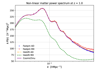
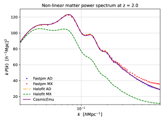
Figure 9: Performance of Halofit (from CLASS code (Blas:2011rf, )) compared to N-body data (from FastPM (Feng:2016yqz, )) for predicting the matter power spectrum for pure adiabatic (AD) and mixed (MX) ICs. For comparison we also plot the curve from CosmicEmu (Moran:2022iwe, ) which is only available for pure adiabatic case. We highlight that Halofit fits N-body data well for adiabatic ICs while grossly misrepresenting the power on mildly nonlinear and even large scales for mixed state. To compare with the performance of EFT we refer the readers to Fig. 2. This figure has been constructed at redshift $z=1$ and $z=2$ with an uncorrelated CDM isocurvature fraction $\alpha=0.25$ for a high blue spectral index $n_{{\rm iso}}=3.75$.

References

- (1) Planck collaboration, P. A. R. Ade, Planck 2015 results. XIII. Cosmological parameters, Astron. Astrophys. 594 (2016) A13, [1502.01589].
- (2) Planck collaboration, Y. Akrami et al., Planck 2018 results. X. Constraints on inflation, Astron. Astrophys. 641 (2020) A10, [1807.06211].
- (3) N. Sailer, E. Castorina, S. Ferraro and M. White, Cosmology at high redshift: a probe of fundamental physics, JCAP 12 (2021) 049, [2106.09713].
- (4) R. Laureijs, J. Amiaux, S. Arduini, J. L. Augueres, J. Brinchmann, R. Cole et al., Euclid definition study report, 2011.
- (5) D. J. Schlegel et al., Astro2020 APC White Paper: The MegaMapper: a Spectroscopic Instrument for the Study of Inflation and Dark Energy, Bull. Am. Astron. Soc. 51 (2019) 229, [1907.11171].
- (6) S. Kasuya and M. Kawasaki, Axion isocurvature fluctuations with extremely blue spectrum, Phys. Rev. D 80 (2009) 023516, [0904.3800].
- (7) D. J. H. Chung and A. Upadhye, Bump in the blue axion isocurvature spectrum, Phys. Rev. D 95 (2017) 023503, [1610.04284].
- (8) D. J. H. Chung and S. C. Tadepalli, Analytic treatment of underdamped axionic blue isocurvature perturbations, Phys. Rev. D 105 (2022) 123511, [2110.02272].
- (9) D. Baumann, A. Nicolis, L. Senatore and M. Zaldarriaga, Cosmological Non-Linearities as an Effective Fluid, JCAP 07 (2012) 051, [1004.2488].
- (10) A. Chudaykin, M. M. Ivanov, O. H. Philcox and M. Simonovic, Nonlinear perturbation theory extension of the boltzmann code CLASS, Physical Review D 102 (sep, 2020) , [2004.10607].
- (11) Y. Feng, M. Chu, U. Seljak and P. McDonald, FastPM: a new scheme for fast simulations of dark matter and haloes, Mon. Not. Roy. Astron. Soc. 463 (2016) 2273–2286, [1603.00476].
- (12) N. Hand, Y. Feng, F. Beutler, Y. Li, C. Modi, U. Seljak et al., nbodykit: an open-source, massively parallel toolkit for large-scale structure, Astron. J. 156 (2018) 160, [1712.05834].
- (13) V. Desjacques, D. Jeong and F. Schmidt, Large-scale galaxy bias, Physics Reports 733 (feb, 2018) 1–193, [1611.09787].
- (14) T. Baldauf, M. Mirbabayi, M. Simonovic and M. Zaldarriaga, LSS constraints with controlled theoretical uncertainties, 1602.00674.
- (15) A. Chudaykin and M. M. Ivanov, Measuring neutrino masses with large-scale structure: Euclid forecast with controlled theoretical error, JCAP 11 (2019) 034, [1907.06666].
- (16) R. Takahashi, M. Sato, T. Nishimichi, A. Taruya and M. Oguri, Revising the Halofit Model for the Nonlinear Matter Power Spectrum, Astrophys. J. 761 (2012) 152, [1208.2701].
- (17) D. J. H. Chung, Large blue isocurvature spectral index signals time-dependent mass, Phys. Rev. D 94 (2016) 043524, [1509.05850].
- (18) H. Kodama and M. Sasaki, Evolution of isocurvature perturbations. II. radiation-dust universe, Int. J. Mod. Phys. A; (United States) 491 (4, 1987) .
- (19) H. Kurki-Suonio, Lecture notes on cosmological perturbation theory: I, .
- (20) J. M. Bardeen, J. R. Bond, N. Kaiser and A. S. Szalay, The statistics of peaks of gaussian random fields, apj 304 (May, 1986) 15.
- (21) G. Efstathiou and J. R. Bond, Isocurvature cold dark matter fluctuations, Mon. Not. Roy. Astron. Soc. 218 (1986) 103–121.
- (22) D. Blas, J. Lesgourgues and T. Tram, The Cosmic Linear Anisotropy Solving System (CLASS) II: Approximation schemes, JCAP 07 (2011) 034, [1104.2933].
- (23) K. R. Moran, K. Heitmann, E. Lawrence, S. Habib, D. Bingham, A. Upadhye et al., The Mira-Titan Universe IV. High-precision power spectrum emulation, Mon. Not. Roy. Astron. Soc. 520 (2023) 3443–3458, [2207.12345].
- (24) J. J. M. Carrasco, M. P. Hertzberg and L. Senatore, The effective field theory of cosmological large scale structures, Journal of High Energy Physics 2012 (sep, 2012) , [1206.2926].
- (25) M. M. Ivanov, Effective Field Theory for Large Scale Structure, 2212.08488.
- (26) R. Angulo, M. Fasiello, L. Senatore and Z. Vlah, On the Statistics of Biased Tracers in the Effective Field Theory of Large Scale Structures, JCAP 09 (2015) 029, [1503.08826].
- (27) F. Bernardeau, S. Colombi, E. Gaztanaga and R. Scoccimarro, Large scale structure of the universe and cosmological perturbation theory, Phys. Rept. 367 (2002) 1–248, [astro-ph/0112551].
- (28) F. Bernardeau, S. Colombi, E. Gaztanaga and R. Scoccimarro, Large-scale structure of the universe and cosmological perturbation theory, Physics Reports 367 (sep, 2002) 1–248, [astro-ph/0112551].
- (29) L. Senatore and M. Zaldarriaga, The IR-resummed Effective Field Theory of Large Scale Structures, JCAP 02 (2015) 013, [1404.5954].
- (30) R. Takahashi, Third Order Density Perturbation and One-loop Power Spectrum in a Dark Energy Dominated Universe, Prog. Theor. Phys. 120 (2008) 549–559, [0806.1437].
- (31) T. Baldauf, L. Mercolli and M. Zaldarriaga, Effective field theory of large scale structure at two loops: The apparent scale dependence of the speed of sound, Physical Review D 92 (dec, 2015) , [1507.02256].
- (32) M. Lewandowski, A. Perko and L. Senatore, Analytic Prediction of Baryonic Effects from the EFT of Large Scale Structures, JCAP 05 (2015) 019, [1412.5049].
- (33) M. P. Hertzberg, Effective field theory of dark matter and structure formation: Semianalytical results, Physical Review D 89 (feb, 2014) , [1208.0839].
- (34) J. J. M. Carrasco, S. Foreman, D. Green and L. Senatore, The 2-loop matter power spectrum and the IR-safe integrand, JCAP 07 (2014) 056, [1304.4946].
- (35) S. Foreman, H. Perrier and L. Senatore, Precision Comparison of the Power Spectrum in the EFTofLSS with Simulations, JCAP 05 (2016) 027, [1507.05326].
- (36) T. Baldauf, E. Schaan and M. Zaldarriaga, On the reach of perturbative descriptions for dark matter displacement fields, JCAP 03 (2016) 017, [1505.07098].
- (37) S. Foreman and L. Senatore, The EFT of Large Scale Structures at All Redshifts: Analytical Predictions for Lensing, JCAP 04 (2016) 033, [1503.01775].
- (38) F. Villaescusa-Navarro, S. Naess, S. Genel, A. Pontzen, B. Wandelt, L. Anderson et al., Statistical properties of paired fixed fields, Astrophys. J. 867 (2018) 137, [1806.01871].
- (39) V. Assassi, D. Baumann, D. Green and M. Zaldarriaga, Renormalized Halo Bias, JCAP 08 (2014) 056, [1402.5916].
- (40) K. C. Chan, R. Scoccimarro and R. K. Sheth, Gravity and large-scale nonlocal bias, Physical Review D 85 (apr, 2012) , [1201.3614].
- (41) A. Eggemeier, R. Scoccimarro, M. Crocce, A. Pezzotta and A. G. Sanchez, Testing one-loop galaxy bias: Power spectrum, Physical Review D 102 (nov, 2020) , [2006.09729].
- (42) A. Eggemeier, R. Scoccimarro, R. E. Smith, M. Crocce, A. Pezzotta and A. G. Sanchez, Testing one-loop galaxy bias: Joint analysis of power spectrum and bispectrum, Physical Review D 103 (jun, 2021) , [2012.06902].
- (43) R. Scoccimarro, E. Sefusatti and M. Zaldarriaga, Probing primordial non-gaussianity with large-scale structure, Physical Review D 69 (may, 2004) , [astro-ph/0312286].
- (44) G. D’Amico, J. Gleyzes, N. Kokron, K. Markovic, L. Senatore, P. Zhang et al., The Cosmological Analysis of the SDSS/BOSS data from the Effective Field Theory of Large-Scale Structure, JCAP 05 (2020) 005, [1909.05271].
- (45) P. McDonald, Clustering of dark matter tracers: Renormalizing the bias parameters, Phys. Rev. D 74 (Nov, 2006) 103512, [astro-ph/0609413].
- (46) L. Senatore, Bias in the Effective Field Theory of Large Scale Structures, JCAP 11 (2015) 007, [1406.7843].
- (47) M. Simonovic, T. Baldauf, M. Zaldarriaga, J. J. Carrasco and J. A. Kollmeier, Cosmological perturbation theory using the FFTLog: formalism and connection to QFT loop integrals, JCAP 04 (2018) 030, [1708.08130].
- (48) Euclid collaboration, A. Blanchard et al., Euclid preparation: VII. Forecast validation for Euclid cosmological probes, Astron. Astrophys. 642 (2020) A191, [1910.09273].
- (49) L. Pozzetti, C. M. Hirata, J. E. Geach, A. Cimatti, C. Baugh, O. Cucciati et al., Modelling the number density of H-alpha emitters for future spectroscopic near-IR space missions, Astron. Astrophys. 590 (2016) A3, [1603.01453].
- (50) Euclid collaboration, S. Ilic et al., Euclid preparation - XV. Forecasting cosmological constraints for the Euclid and CMB joint analysis, Astron. Astrophys. 657 (2022) A91, [2106.08346].
- (51) A. E. Shapley, Physical properties of galaxies from , Annual Review of Astronomy and Astrophysics 49 (2011) 525–580, [https://doi.org/10.1146/annurev-astro-081710-102542].
- (52) S. Ferraro et al., Inflation and Dark Energy from Spectroscopy at , Bull. Am. Astron. Soc. 51 (2019) 72, [1903.09208].
- (53) T. Baldauf, U. Seljak, V. Desjacques and P. McDonald, Evidence for Quadratic Tidal Tensor Bias from the Halo Bispectrum, Phys. Rev. D 86 (2012) 083540, [1201.4827].
- (54) A. Eggemeier, R. Scoccimarro and R. E. Smith, Bias loop corrections to the galaxy bispectrum, Physical Review D 99 (jun, 2019) , [1812.03208].
- (55) T. Lazeyras, C. Wagner, T. Baldauf and F. Schmidt, Precision measurement of the local bias of dark matter halos, JCAP 02 (2016) 018, [1511.01096].
- (56) V. Yankelevich and C. Porciani, Cosmological information in the redshift-space bispectrum, Mon. Not. Roy. Astron. Soc. 483 (2019) 2078–2099, [1807.07076].
- (57) E. Di Dio, R. Durrer, R. Maartens, F. Montanari and O. Umeh, The Full-Sky Angular Bispectrum in Redshift Space, JCAP 04 (2019) 053, [1812.09297].
- (58) T. Baldauf, U. Seljak, R. E. Smith, N. Hamaus and V. Desjacques, Halo stochasticity from exclusion and nonlinear clustering, Phys. Rev. D 88 (2013) 083507, [1305.2917].
- (59) T. Lazeyras and F. Schmidt, A robust measurement of the first higher-derivative bias of dark matter halos, JCAP 11 (2019) 041, [1904.11294].
- (60) O. H. E. Philcox, M. M. Ivanov, G. Cabass, M. Simonovic, M. Zaldarriaga and T. Nishimichi, Cosmology with the redshift-space galaxy bispectrum monopole at one-loop order, Phys. Rev. D 106 (2022) 043530, [2206.02800].
- (61) J. Chluba and D. Grin, CMB spectral distortions from small-scale isocurvature fluctuations, Monthly Notices of the Royal Astronomical Society 434 (jul, 2013) 1619–1635, [1304.4596].
- (62) N. Lee and Y. Ali-Haimoud, Probing small-scale baryon and dark matter isocurvature perturbations with cosmic microwave background anisotropies, Phys. Rev. D 104 (2021) 103509, [2108.07798].
- (63) T. Sekiguchi, H. Tashiro, J. Silk and N. Sugiyama, Cosmological signatures of tilted isocurvature perturbations: reionization and 21cm fluctuations, JCAP 03 (2014) 001, [1311.3294].
- (64) Y. Takeuchi and S. Chongchitnan, Constraining isocurvature perturbations with the 21 cm emission from minihaloes, Mon. Not. Roy. Astron. Soc. 439 (2014) 1125–1135, [1311.2585].
- (65) T. Minoda, S. Yoshiura and T. Takahashi, Probing isocurvature perturbations with 21-cm global signal in the light of hera result, Phys. Rev. D 105 (2022) 083523, [2112.15135].
- (66) I. Esteban, A. H. G. Peter and S. Y. Kim, Milky Way satellite velocities reveal the Dark Matter power spectrum at small scales, 2306.04674.
- (67) J. Ryan, B. Stevenson, C. Trendafilova and J. Meyers, Beyond Fisher forecasting for cosmology, Phys. Rev. D 107 (2023) 103506, [2211.06534].
- (68) D. Baumann and D. Green, The power of locality: primordial non-Gaussianity at the map level, JCAP 08 (2022) 061, [2112.14645].
- (69) S. Dodelson and F. Schmidt, Modern Cosmology. Elsevier Science, 2020.
- (70) D. Coe, Fisher Matrices and Confidence Ellipses: A Quick-Start Guide and Software, 0906.4123.
- (71) J. LESGOURGUES and S. PASTOR, Massive neutrinos and cosmology, Physics Reports 429 (jul, 2006) 307–379, [astro-ph/0603494].
- (72) N. Bellomo, J. L. Bernal, G. Scelfo, A. Raccanelli and L. Verde, Beware of commonly used approximations. Part I. Errors in forecasts, JCAP 10 (2020) 016, [2005.10384].
- (73) B. Joachimi and A. N. Taylor, Forecasts of non-Gaussian parameter spaces using Box-Cox transformations, Mon. Not. Roy. Astron. Soc. 416 (2011) 1010–1022, [1103.3370].
- (74) E. Sellentin, M. Quartin and L. Amendola, Breaking the spell of Gaussianity: forecasting with higher order Fisher matrices, Mon. Not. Roy. Astron. Soc. 441 (2014) 1831–1840, [1401.6892].
- (75) E. Sellentin, A fast, always positive definite and normalizable approximation of non-Gaussian likelihoods, Mon. Not. Roy. Astron. Soc. 453 (2015) 893–898, [1506.04866].
- (76) L. Amendola and E. Sellentin, Optimizing parameter constraints: a new tool for Fisher matrix forecasts, Mon. Not. Roy. Astron. Soc. 457 (2016) 1490–1495, [1602.01746].
- (77) L. Wolz, M. Kilbinger, J. Weller and T. Giannantonio, On the validity of cosmological fisher matrix forecasts, Journal of Cosmology and Astroparticle Physics 2012 (sep, 2012) 009–009, [1205.3984].
- (78) D. Wadekar, M. M. Ivanov and R. Scoccimarro, Cosmological constraints from BOSS with analytic covariance matrices, Phys. Rev. D 102 (2020) 123521, [2009.00622].
- (79) P. Reimberg, F. Bernardeau, T. Nishimichi and M. Rizzato, Failures of Halofit model for computation of Fisher Matrices, 1811.02976.