Analytical Evaluation of Elastic Lepton-Proton Two-Photon Exchange
in Chiral Perturbation Theory

Abstract

We present an exact evaluation of the two-photon exchange contribution to the elastic lepton-proton scattering process at low-energies using heavy baryon chiral perturbation theory. The evaluation is performed including next-to-leading order accuracy. This exact analytical evaluation contains all soft and hard two-photon exchanges and we identify the contributions missing in a soft-photon approximation approach. We evaluate the infrared divergent four-point box diagrams analytically using dimensional regularization. We also emphasize the differences between muon-proton and electron-proton scatterings relevant to the MUSE kinematics due to lepton mass differences.

I INTRODUCTION

Scattering of light leptons off hadron targets has been the most time-honored precision tool to study the internal composite structure and dynamics of hadrons since the pioneering work of Hofstadter and McAllister Hofstadter:1955ae . The point-like nature of the leptons makes them ideal probes of the hadronic electromagnetic structure. Despite a century-long endeavor to understand the basic nucleon structure, fundamental gaps in our knowledge still persist.

An accurate determination of the proton’s electromagnetic form factors and parton distributions is known to shed much light on the constituent spin, charge, and magnetic distributions. However, various systematic analyses of high-precision lepton-proton ($\ell^{\pm}$p) elastic scattering data, providing the cleanest possible information on the proton’s internal structure, have brought forth several discrepancies in the recent past which questions our conventional notion regarding the proton’s structure as revealed from the standard treatments of QED and QCD. A well-known discrepancy is the stark difference in the measured value of the proton’s electric ($G^{p}_{E}$) to magnetic ($G^{p}_{M}$) form factor ratio ($G^{p}_{E}/G^{p}_{M}$) at momentum transfers $Q^{2}$ beyond $\gtrsim 1$ (GeV/c)² between two different popular experimental methodologies, namely, the Rosenbluth Separation Rosenbluth:1950yq and Recoil Polarization Transfer Akhiezer:1974em ; Arnold:1980zj ; Gayou:2001qt techniques (also see, Refs. Jones:1999rz ; Perdrisat:2006hj ; Punjabi:2015bba ; Puckett:2010 for more details). A resolution to this “form factor puzzle” necessitates a closer investigation of the so-called Two-Photon Exchange (TPE) contributions to the radiative corrections to the elastic $\ell^{\pm}$p cross-section (for prominent past works and reviews, see e.g., Refs. Arrington:2003 ; Guichon:2003 ; Blunden:2003sp ; Rekalo:2004wa ; Blunden:2005ew ; Carlson:2007sp ; Arrington:2011 ). The TPE corrections give an additional higher-order contribution to the well-known leading order (LO) Born approximation contribution arising from the One-Photon Exchange (OPE) diagram which was assumed to dominate this electromagnetic scattering process at small momentum transfers.

Likewise, there exists yet another puzzling scenario in regard to low-momentum transfers where the TPE consideration may prove to be a crucial game changer. This concerns the proton’s charge radius, as obtained from the slope of $G^{p}_{E}$ at $Q^{2}=0$. There exist two exclusive means to determine the charge radius, namely, via scattering processes and via atomic spectroscopy. In particular, the muonic Lamb-shift measurements of the rms charge radius by the CREMA Collaboration Pohl:2010zza ; Pohl:2013 are strikingly inconsistent with the prior CODATA recommended value  Mohr:2012tt . Such a discrepancy, the so-called “proton radius puzzle”, has been an agenda of serious scientific contention over the last decade since its inception in 2013 Antognini:1900ns ; Bernauer:2014 ; Carlson:2015 ; Bernauer:2020ont . Despite the flurry of ingenious ideas and techniques introduced to fix the conundrum, the resolution of this discrepancy remained unsettled thus far. We refer the reader to the recent status report as presented in Ref. Gao:2021sml . With no apparent fundamental flaws either conceptually or in the measurement process to explain this incongruity, the TPE processes may be singularly implicated as culpable under circumstantial evidence, vis-a-vis, the form factor puzzle Arrington:2003 ; Guichon:2003 ; Blunden:2003sp ; Rekalo:2004wa ; Blunden:2005ew ; Carlson:2007sp ; Arrington:2011 . It is conceivable that a rigorous evaluation of the TPE effects could potentially resolve both the form factor and radius discrepancies. Given the growing consensus in this regard, many new theoretical works on TPE studies have recently appeared in the literature Kivel:2012vs ; Lorenz:2014yda ; Tomalak:2014sva ; Tomalak:2014dja ; Tomalak:2015aoa ; Tomalak:2015hva ; Tomalak:2016vbf ; Tomalak:2017npu ; Koshchii:2017dzr ; Tomalak:2018jak ; Talukdar:2019dko ; Peset:2021iul ; Talukdar:2020aui ; Kaiser:2022pso ; Guo:2022kfo .

Of the several newly commissioned high-precision scattering experiments Bernauer:2020ont , the ongoing MUSE Collaboration project at PSI Gilman:2013eiv is one such endeavor, uniquely designed to simultaneously scatter leptons ($\ell^{-}\equiv e^{-},\,\mu^{-}$) as well as anti-leptons ($\ell^{+}\equiv e^{+},\,\mu^{+}$) off a proton target. One specialty of MUSE will be its uniqueness in pinning down the charge-odd contributions to the unpolarized lepton-proton ($\ell^{\pm}$p $\to\ell^{\pm}$p) scattering, which arguably includes the TPE as the dominant process. Nevertheless, isolating the charge-odd contributions does not necessarily preclude other competing low-energy chiral-radiative contributions Talukdar:2020aui in affecting the extraction of the pure TPE loop contributions. In particular, the recent estimation Talukdar:2020aui of the “soft” bremsstrahlung ($\ell^{\pm}$p $\to\ell^{\pm}$p$\,\gamma^{*}_{\rm soft}$) corrections to next-to-leading order (NLO) in heavy baryon chiral perturbation theory (HB$\chi$PT) Gasser:1982ap ; Jenkins:1990jv ; Bernard:1992qa ; Ecker:1994pi ; Bernard:1995dp revealed novel chiral-odd constituents large enough (and of opposite sign) to supersede the TPE effects pertinent to the MUSE kinematics. Given that the TPE processes are major sources of systematic uncertainty, their accurate theoretical estimation is of pivotal interest for the purpose of precision analysis of the future MUSE data aimed at sub-percentage accuracy.

Since the inception of the radius puzzle, the importance of low-energy TPE contributions has been extensively explored via diverse approaches such as QED-inspired hadronic models Tomalak:2014dja ; Tomalak:2015aoa ; Tomalak:2015hva ; Koshchii:2017dzr ; Guo:2022kfo , Dispersion techniques Lorenz:2014yda ; Tomalak:2014sva ; Tomalak:2016vbf ; Tomalak:2017npu ; Tomalak:2018jak ; Guo:2022kfo , and Effective Field Theories (EFTs) such as Non-Relativistic Quantum Electrodynamics (NRQED) Peset:2021iul , Baryon Chiral Perturbation Theory (B$\chi$PT) Cao:2021nhm and HB$\chi$PT Talukdar:2019dko ; Talukdar:2020aui . It is well-known that restricting to the low-energy regime, the TPE with elastic proton intermediate state yields the dominant contribution to the radiative corrections Blunden:2003sp . Besides the proton, the inclusion of other excited nucleon intermediate states, such as the spin-isospin quartet of $\Delta(1232)$ resonances, can yield interesting results Bernauer:2014 relevant to the MUSE kinematics that leads to a better understanding of the non-perturbative aspects of the TPE contributions Kondratyuk:2005kk . The TPE loop diagrams which have been evaluated in the past for a wide range of intermediate to high momentum transfers Christy:2021snt are either known to be model-dependent or used unwarranted simplifications (generally referred to as soft photon approximation or SPA Tsai:1961zz ) in the treatment of the intricate four-point functions, (see e.g., Refs. Koshchii:2017dzr ; Tomalak:2014dja ). In this work, we present the evaluation of the TPE loop contributions using HB$\chi$PT without taking recourse to SPA methods.

The outline of the paper is as follows. In Sec. II, after a brief discussion of the HB$\chi$PT Lagrangian needed for our intended accuracy, namely, including interactions that at next-to-leading order (NLO) in the power counting, we introduce the possible topologies of the TPE loop diagrams that contribute at LO and NLO. In Sec. III, we discuss the amplitudes of these loop diagrams and their contributions to the elastic cross-section. In Sec. IV, we discuss our numerical results and compare them with other works. Finally, we present our summary and conclusions in Sec. V. Appendix A contains the notations of the various generic two-, three- and four-point integral functions that contribute to the TPE corrections to the cross-section. In this work, all such relevant integrals have been evaluated exactly, and their analytical expressions are collected in Appendix B.

II TPE diagrams in HB$\chi$PT

In this work, we evaluate the LO and NLO TPE contributions to lepton-proton elastic scattering cross-section using HB$\chi$PT, where only parts of the LO and NLO chiral Lagrangian contribute. In particular, the pion degrees of freedom that appear only via the next-to-next-to-leading order (NNLO) loop diagrams are absent in our current accuracy. This means that in our Lagrangian the non-linear Goldstone field $u=\sqrt{U}$ effectively contributes as the identity matrix in two-dimensional isospin space, namely, $u\mapsto{\mathbb{I}}_{2\times 2}$. Consequently, the relevant LO and NLO parts of the chiral Lagrangian become

$$\mathcal{L}^{(0)}_{\pi N}=\overline{N}(iv\cdot D+g_{A}S\cdot u)N\,,$$ (1)

and

$$\mathcal{L}^{(1)}_{\pi N}=\overline{N}\left\{\frac{1}{2M}(v\cdot D)^{2}-\frac{1}{2M}D\cdot D+...\right\}N\,,$$ (2)

respectively, where $N=(\rm{p\,\,n})^{\rm T}$ is the heavy nucleon spin-isospin doublet spinor field, $g_{A}=1.267$ is axial coupling constant of the nucleon, and $v_{\mu}$ and $S_{\mu}$ are the nucleon velocity and spin four-vectors satisfying the condition, $v\cdot S=0$. Here, the standard choice is $v=(1,{\bf 0})$ such that $S=(0,\boldsymbol{\sigma}/2)$. Furthermore, the gauge covariant derivative is

$$D_{\mu}=\partial_{\mu}+\Gamma_{\mu}-iv^{(s)}_{\mu}\,,$$ (3)

with the chiral connection given by

$$\Gamma_{\mu}=\frac{1}{2}[u^{\dagger}(\partial_{\mu}-ir_{\mu})u+u(\partial_{\mu}-il_{\mu})u^{\dagger}]\,,$$ (4)

and the chiral vielbein is $u_{\mu}=iu^{\dagger}\nabla_{\mu}Uu^{\dagger}$, where

$$\quad\nabla_{\mu}U=\partial_{\mu}U-ir_{\mu}U+iUl_{\mu}\,.$$ (5)

Here, $l_{\mu}$ and $r_{\mu}$ are external iso-vector chiral source fields, which in our case are given by the photon field, namely, $r_{\mu}=l_{\mu}=-e\frac{\tau^{3}}{2}A_{\mu}$, with $\tau^{3}$ being the third Pauli isospin matrix. Finally, $v_{\mu}^{(s)}=-e\frac{I}{2}A_{\mu}$ is the external iso-scalar vector source field.

Figure 1: TPE diagrams of $\mathcal{O}(\alpha^{2})$ which contribute to the $\mathcal{O}(\alpha^{3})$ elastic cross-section. The thick, thin, and wiggly lines denote proton, lepton, and photon propagators, respectively. The blobs and crosses denote NLO insertions of the proton-photon vertices and proton propagators, respectively.

Figure 1 shows all relevant TPE diagrams up-to-and-including NLO chiral order. The first two diagrams, namely, the box diagram (a) and the crossed-box diagram (b) are of LO where both the photon-proton vertices as well as the proton propagator stem from the LO Lagrangian. However, these two LO diagrams also contain ${\mathcal{O}}(1/M)$ parts originating from the proton propagators (see below) which are kinematically suppressed. In $\chi$PT the perturbative chiral expansion is determined in terms of powers of the expansion parameter $Q/\Lambda_{\chi}$, where $Q$ is a generic momentum scale of the process and $\Lambda_{\chi}\approx 1$ GeV/c is the breakdown scale of the theory. Since the value of $\Lambda_{\chi}$ is approximately equal to the proton’s mass $M$, the HB$\chi$PT additionally incorporates a non-perturbative power or recoil correction of the interaction vertices and propagators via an expansion in powers of the inverse proton’s mass, namely, $Q/M\sim Q/\Lambda_{\chi}$. It is also important to formally distinguish such dynamical recoil corrections from the naive kinematical recoil corrections. Thus, for instance, the difference in incoming lepton and outgoing lepton energies, $E-E^{\prime}=-Q^{2}/(2M)$, and the corresponding lepton velocities, $\beta-\beta^{\prime}=-Q^{2}(1-\beta^{2})/(2ME\beta)+{\mathcal{O}}(1/M^{2})$, are interpreted as kinematic recoil corrections of order $1/M$. Nevertheless, in practice, such corrections are also referred to as NLO corrections. Consequently, diagrams (a) and (b) are not “true LO” chiral contributions since they contain order $1/M$ “NLO contributions” from the proton propagator, e.g., $v\cdot p_{p}\approx-p^{2}_{p}/(2M)+{\mathcal{O}}(1/M^{2})$, where $p_{p}$ is a generic small off-shell four-momentum of the proton which is related to the corresponding full four-momentum in the heavy baryon formalism by the relation, $P^{\mu}=Mv^{\mu}+p^{\mu}_{p}$. Next, the diagrams (c), (d), (e), and (f) are genuine NLO chiral order diagrams since they contain one NLO vertex, i.e., one photon-proton vertex is taken from NLO chiral Lagrangian whereas the propagators in each of these diagrams are taken from LO chiral Lagrangian. Likewise, the diagrams (g) and (h) are also genuine NLO box and crossed-box diagrams where the proton propagator in each diagram is derived from NLO chiral Lagrangian whereas the proton-photon vertices are taken from LO chiral Lagrangian. Finally, the triangular-shaped seagull diagram (i) contains an NLO vertex of $\mathcal{O}(e^{2})$ with no proton intermediate state. The explicit amplitude for each of the TPE diagrams is given by the following expressions:

$${\mathcal{M}}^{(a)}_{\rm box}\! = \!e^{4}\int\!\frac{{\rm d}^{4}k}{(2\pi)^{4}i}\frac{\left[\bar{u}(p^{\prime})\gamma^{\mu}(\not{\!p}\,-\not{\!k}+\,m_{l})\gamma^{\nu}u(p)\right]\,\left[\chi^{\dagger}(p_{p}^{\prime})v_{\mu}v_{\nu}\chi(p_{p})\right]}{(k^{2}+i0)\,[(Q-k)^{2}+i0]\,(k^{2}-2k\cdot p+i0)\,(v\cdot k+v\cdot p_{p}+i0)}\,,$$ (6)

$${\mathcal{M}}^{(b)}_{\rm xbox}\! = \!e^{4}\int\!\frac{{\rm d}^{4}k}{(2\pi)^{4}i}\frac{\left[\bar{u}(p^{\prime})\gamma^{\mu}(\not{\!p}\,-\not{\!k}+\,m_{l})\gamma^{\nu}u(p)\right]\,\left[\chi^{\dagger}(p_{p}^{\prime})v_{\mu}v_{\nu}\chi(p_{p})\right]}{(k^{2}+i0)\,[(Q-k)^{2}+i0]\,(k^{2}-2k\cdot p+i0)\,(-v\cdot k+v\cdot p^{\prime}_{p}+i0)}\,,$$ (7)

$${\mathcal{M}}^{(c)}_{\rm box}\! = \!\frac{e^{4}}{2M}\int\!\frac{{\rm d}^{4}k}{(2\pi)^{4}i}\frac{\left[\bar{u}(p^{\prime})\gamma^{\mu}(\not{\!p}\,-\not{\!k}+\,m_{l})\gamma^{\nu}u(p)\right]\,\left[\chi^{\dagger}(p_{p}^{\prime})\{v_{\mu}(k+2p_{p})_{\nu}-v_{\mu}v_{\nu}v\cdot(k+2p_{p})\}\chi(p_{p})\right]}{(k^{2}+i0)\,[(Q-k)^{2}+i0]\,(k^{2}-2k\cdot p+i0)\,(v\cdot k+v\cdot p_{p}+i0)}\,,$$ (8)

$${\mathcal{M}}^{(d)}_{\rm xbox}\! = \!\frac{e^{4}}{2M}\int\!\frac{{\rm d}^{4}k}{(2\pi)^{4}i}\frac{\left[\bar{u}(p^{\prime})\gamma^{\mu}(\not{\!p}\,-\not{\!k}+\,m_{l})\gamma^{\nu}u(p)\right]\,\left[\chi^{\dagger}(p_{p}^{\prime})\{v_{\nu}(p_{p}+p_{p}^{\prime}-k)_{\mu}-v_{\mu}v_{\nu}v\cdot(p_{p}+p_{p}^{\prime}-k)\}\chi(p_{p})\right]}{(k^{2}+i0)\,[(Q-k)^{2}+i0]\,(k^{2}-2k\cdot p+i0)\,(v\cdot p^{\prime}_{p}-v\cdot k+i0)}\,,\qquad\,$$ (9)

$${\mathcal{M}}^{(e)}_{\rm box}\! = \!\frac{e^{4}}{2M}\int\!\frac{{\rm d}^{4}k}{(2\pi)^{4}i}\frac{\left[\bar{u}(p^{\prime})\gamma^{\mu}(\not{\!p}\,-\not{\!k}+\,m_{l})\gamma^{\nu}u(p)\right]\,\left[\chi^{\dagger}(p_{p}^{\prime})\{v_{\nu}(p_{p}+p_{p}^{\prime}+k)_{\mu}-v_{\mu}v_{\nu}v\cdot(p_{p}+p_{p}^{\prime}+k)\}\chi(p_{p})\right]}{(k^{2}+i0)\,[(Q-k)^{2}+i0]\,(k^{2}-2k\cdot p+i0)\,(v\cdot p_{p}+v\cdot k+i0)}\,,\qquad\,$$ (10)

$${\mathcal{M}}^{(f)}_{\rm xbox}\! = \!\frac{e^{4}}{2M}\int\!\frac{{\rm d}^{4}k}{(2\pi)^{4}i}\frac{\left[\bar{u}(p^{\prime})\gamma^{\mu}(\not{\!p}\,-\not{\!k}+\,m_{l})\gamma^{\nu}u(p)\right]\,\left[\chi^{\dagger}(p_{p}^{\prime})\{v_{\mu}(2p_{p}^{\prime}-k)_{\nu}-v_{\mu}v_{\nu}v\cdot(2p_{p}^{\prime}-k)\}\chi(p_{p})\right]}{(k^{2}+i0)\,[(Q-k)^{2}+i0]\,(k^{2}-2k\cdot p+i0)\,(v\cdot p^{\prime}_{p}-v\cdot k+i0)}\,,$$ (11)

$$\mathcal{M}^{(g)}_{\rm box}\! = \!\frac{e^{4}}{2M}\int\!\frac{{\rm d}^{4}k}{(2\pi)^{4}i}\frac{\left[\bar{u}(p^{\prime})\gamma^{\mu}(\not{\!p}\,-\not{\!k}+\,m_{l})\gamma^{\nu}u(p)\right]\,\left[\chi^{\dagger}(p_{p}^{\prime})v_{\mu}v_{\nu}\chi(p_{p})\right]}{(k^{2}+i0)\,[(Q-k)^{2}+i0]\,(k^{2}-2k\cdot p+i0)}\left(1-\frac{(p_{p}+k)^{2}}{(v\cdot p_{p}+v\cdot k+i0)^{2}}\right)\,,$$ (12)

$${\mathcal{M}}^{(h)}_{\rm xbox}\! = \!\frac{e^{4}}{2M}\int\!\frac{{\rm d}^{4}k}{(2\pi)^{4}i}\frac{\left[\bar{u}(p^{\prime})\gamma^{\mu}(\not{\!p}\,-\not{\!k}+\,m_{l})\gamma^{\nu}u(p)\right]\,\left[\chi^{\dagger}(p_{p}^{\prime})v_{\mu}v_{\nu}\chi(p_{p})\right]}{(k^{2}+i0)\,[(Q-k)^{2}+i0]\,(k^{2}-2k\cdot p+i0)}\left(1-\frac{(p^{\prime}_{p}-k)^{2}}{(v\cdot p^{\prime}_{p}-v\cdot k+i0)^{2}}\right)\,,$$ (13)

$${\mathcal{M}}^{(i)}_{\rm seagull}\! = \!\frac{2e^{4}}{2M}\int\!\frac{{\rm d}^{4}k}{(2\pi)^{4}i}\frac{\left[\bar{u}(p^{\prime})\gamma^{\mu}(\not{\!p}\,-\not{\!k}+\,m_{l})\gamma^{\nu}u(p)\right]\,\left[\chi^{\dagger}(p_{p}^{\prime})(v_{\mu}v_{\nu}-g_{\mu\nu})\chi(p_{p})\right]}{(k^{2}+i0)\,[(Q-k)^{2}+i0]\,(k^{2}-2k\cdot p+i0)}\,,$$ (14)

where $u(p)$ and $\bar{u}(p^{\prime})$ are the incoming and outgoing lepton Dirac spinors, and $\chi(p_{p})$ and $\chi^{\dagger}(p_{p}^{\prime})$ are the corresponding non-relativistic proton Pauli spinors. We have used the fact that the proton propagators up-to-and-including NLO for the box and crossed-box TPE loops diagrams are respectively given as

$$iS^{(1/M)}_{\rm full}(p_{p}+k)\! = \!\frac{i}{v\cdot(p_{p}+k)+i0}+\frac{i}{2M}\left[1-\frac{(p_{p}+k)^{2}}{(v\cdot p_{p}+v\cdot k+i0)^{2}}\right]+{\cal O}(M^{-2})\,,$$

$$iS^{(1/M)}_{\rm full}(p^{\prime}_{p}-k)\! = \!\frac{i}{v\cdot(p^{\prime}_{p}-k)+i0}+\frac{i}{2M}\left[1-\frac{(p^{\prime}_{p}-k)^{2}}{(v\cdot p^{\prime}_{p}-v\cdot k+i0)^{2}}\right]+{\cal O}(M^{-2})\,.$$ (15)

Next, examining the possible cancellations of contributions at the amplitude level, the following comments are in order:

• First, it is convenient for us to use the lab-frame kinematics where the initial proton is at rest, i.e., $p_{p}=0$, which means that the four-momentum transfer is $Q=p^{\prime}_{p}-p_{p}=p^{\prime}_{p}$.

• Second, since we observe that $v\cdot Q=E-E^{\prime}=-Q^{2}/(2M)\sim{\mathcal{O}}(1/M)$, this difference can therefore be neglected in the numerators of the NLO amplitudes

  $$\mathcal{M}^{(c)}_{\rm box}\,,\,\,\mathcal{M}^{(d)}_{\rm box}\,,\,\,\mathcal{M}^{(e)}_{\rm box}\,,\,\,\text{and}\,\,\,\mathcal{M}^{(f)}_{\rm xbox}\,,$$

  as they give rise to higher-order contributions. What remains in the numerators of these four amplitudes following the factor $v_{\mu}v_{\nu}$ are the terms $v\cdot k$, only. However, it is important to retain the $v\cdot Q$ terms in the denominators of the proton propagators for consistent evaluation of the loop integrals. In many cases, they serve as natural regulators against infrared (IR) divergences. Nevertheless, as stated, we may ignore all $v\cdot p_{p}^{\prime}=v\cdot Q$ terms in the NLO expressions after evaluations of the integrals, only.

Consequently, when we sum these amplitudes, the terms containing the factors $v_{\mu}v_{\nu}$ in the four NLO amplitudes of $\mathcal{M}^{(c)}_{\rm box}$, $\mathcal{M}^{(d)}_{\rm xbox}$, $\mathcal{M}^{(e)}_{\rm box}$ and $\mathcal{M}^{(f)}_{\rm xbox}$, cancel with the two $v_{\mu}v_{\nu}$ terms with coefficient 1 (within the braces) of $\mathcal{M}^{(g)}_{\rm box}$ and $\mathcal{M}^{(h)}_{\rm xbox}$, plus the $v_{\mu}v_{\nu}$ term in the seagull amplitude $\mathcal{M}^{(i)}_{\rm seagull}$. After such partial cancellations between the NLO amplitudes, the remaining parts of the NLO box diagrams (c), (e), and (g), and the seagull diagram (i), along with the unaltered LO amplitude (a) are given in the lab-frame as follows:

$$i{\mathcal{M}}^{(a)}_{\rm box}\! = \!e^{4}\int\frac{{\rm d}^{4}k}{(2\pi)^{4}}\frac{\left[\bar{u}(p^{\prime})\gamma^{\mu}(\not{\!p}-\not{\!k}+\,m_{l})\gamma^{\nu}u(p)\right]\,\left[\chi^{\dagger}(p_{p}^{\prime})v_{\mu}v_{\nu}\chi(p_{p})\right]}{(k^{2}+i0)\,[(Q-k)^{2}+i0]\,(k^{2}-2k\cdot p+i0)\,(v\cdot k+i0)}\,,$$

$$i\widetilde{\mathcal{M}}^{(c)}_{\rm box}\! = \!\frac{e^{4}}{2M}\int\frac{{\rm d}^{4}k}{(2\pi)^{4}}\frac{\left[\bar{u}(p^{\prime})\gamma^{\mu}(\not{\!p}-\not{\!k}+\,m_{l})\gamma^{\nu}u(p)\right]\,\left[\chi^{\dagger}(p^{\prime}_{p}){v_{\mu}k_{\nu}}\chi(p_{p})\right]}{(k^{2}+i0)\,[(Q-k)^{2}+i0]\,(k^{2}-2k\cdot p+i0)\,(v\cdot k+i0)}\,,$$

$$i\widetilde{\mathcal{M}}^{(e)}_{\rm box}\! = \!\frac{e^{4}}{2M}\int\frac{{\rm d}^{4}k}{(2\pi)^{4}}\frac{\left[\bar{u}(p^{\prime})\gamma^{\mu}(\not{\!p}-\not{\!k}+\,m_{l})\gamma^{\nu}u(p)\right]\,\left[\chi^{\dagger}(p^{\prime}_{p}){v_{\nu}(k+Q)_{\mu}}\chi(p_{p})\right]}{(k^{2}+i0)\,[(Q-k)^{2}+i0]\,(k^{2}-2k\cdot p+i0)\,(v\cdot k+i0)}\,,$$

$$i\widetilde{\mathcal{M}}^{(g)}_{\rm box}\! = \!\frac{e^{4}}{2M}\int\frac{{\rm d}^{4}k}{{2\pi}^{4}}\frac{\left[\bar{u}(p^{\prime})\gamma^{\mu}(\not{\!p}-\not{\!k}+\,m_{l})\gamma^{\nu}u(p)\right]\,\left[\chi^{\dagger}(p^{\prime}_{p})v_{\mu}v_{\nu}\chi(p_{p})\right]}{(k^{2}+i0)\,[(Q-k)^{2}+i0]\,(k^{2}-2k\cdot p+i0)}\Bigg{(}-\frac{k^{2}}{(v\cdot k+i0)^{2}}\Bigg{)}$$

$$= \!-\,\frac{e^{4}}{2M}\int\frac{{\rm d}^{4}k}{{2\pi}^{4}}\frac{\left[\bar{u}(p^{\prime})\gamma^{\mu}(\not{\!p}-\not{\!k}+\,m_{l})\gamma^{\nu}u(p)\right]\,\left[\chi^{\dagger}(p^{\prime}_{p})v_{\mu}v_{\nu}\chi(p_{p})\right]}{[(Q-k)^{2}+i0]\,(k^{2}-2k\cdot p+i0)\,(v\cdot k+i0)^{2}}\,,$$

$$i\widetilde{\mathcal{M}}^{(i)}_{\rm seagull}\! = \!-\,\frac{e^{4}}{M}\!\!\int\!\!\frac{{\rm d}^{4}k}{(2\pi)^{4}}\frac{\left[\bar{u}(p^{\prime})\gamma^{\mu}(\not{\!p}-\not{\!k}+\,m_{l})\gamma_{\mu}u(p)\right]\,\left[\chi^{\dagger}(p_{p}^{\prime})\,\chi(p_{p})\right]}{(k^{2}+i0)\,[(Q-k)^{2}+i0]\,(k^{2}-2k\cdot p+i0)}\,.$$ (16)

Regarding the other amplitudes for the crossed-box diagrams, it is convenient to shift the integration variable $k$ by means of the transformation $k\rightarrow-k+Q$, which yields the following expressions:

$$i{\mathcal{M}}^{(b)}_{\rm xbox}\! = \!e^{4}\int\frac{{\rm d}^{4}k}{(2\pi)^{4}}\frac{\left[\bar{u}(p^{\prime})\gamma^{\mu}(\not{\!p}+\not{\!k}-\not{\!Q}+\,m_{l})\gamma^{\nu}u(p)\right]\,\left[\chi^{\dagger}(p_{p}^{\prime})v_{\mu}v_{\nu}\chi(p_{p})\right]}{(k^{2}+i0)\,[(Q-k)^{2}+i0]\,(k^{2}+2k\cdot p^{\prime}+i0)\,(v\cdot k+i0)}\,,$$

$$i\widetilde{\mathcal{M}}^{(d)}_{\rm xbox}\! = \!\frac{e^{4}}{2M}\int\frac{{\rm d}^{4}k}{(2\pi)^{4}}\frac{\left[\bar{u}(p^{\prime})\gamma^{\mu}(\not{\!p}+\not{\!k}-\not{\!Q}+\,m_{l})\gamma^{\nu}u(p)\right]\,\left[\chi^{\dagger}(p^{\prime}_{p}){v_{\nu}k_{\mu}}\chi(p_{p})\right]}{(k^{2}+i0)\,[(Q-k)^{2}+i0]\,(k^{2}+2k\cdot p^{\prime}+i0)\,(v\cdot k+i0)}\,,$$

$$i\widetilde{\mathcal{M}}^{(f)}_{\rm xbox}\! = \!\frac{e^{4}}{2M}\int\frac{{\rm d}^{4}k}{(2\pi)^{4}}\frac{\left[\bar{u}(p^{\prime})\gamma^{\mu}(\not{\!p}+\not{\!k}-\not{\!Q}+\,m_{l})\gamma^{\nu}u(p)\right]\,\left[\chi^{\dagger}(p^{\prime}_{p}){v_{\mu}(k+Q)_{\nu}}\chi(p_{p})\right]}{(k^{2}+i0)\,[(Q-k)^{2}+i0]\,(k^{2}+2k\cdot p^{\prime}+i0)\,(v\cdot k+i0)}\,,$$

$$i\widetilde{\mathcal{M}}^{(h)}_{\rm xbox}\! = \!-\,\frac{e^{4}}{2M}\int\frac{{\rm d}^{4}k}{{2\pi}^{4}}\frac{\left[\bar{u}(p^{\prime})\gamma^{\mu}(\not{\!p}+\not{\!k}-\not{\!Q}+\,m_{l})\gamma^{\nu}u(p)\right]\,\left[\chi^{\dagger}(p^{\prime}_{p})v_{\mu}v_{\nu}\chi(p_{p})\right]}{[(k-Q)^{2}+i0]\,(k^{2}+2k\cdot p^{\prime}+i0)\,(v\cdot k+i0)^{2}}\,.$$ (17)

The above TPE amplitudes include only LO and NLO amplitude contributions, i.e., we neglect all higher-order contributions. These diagrams constitute the radiative corrections to the LO Born amplitude and contribute to the elastic unpolarized lepton-proton scattering cross-section. Their contribution to the cross-section is obtained via the interference of these TPE amplitudes with the LO Born diagram Talukdar:2019dko ; Talukdar:2020aui . In the following section, we present the complete analytical evaluation of the above TPE contributions to the cross-section up-to-and-including NLO in HB$\chi$PT without resorting to any kind of approximation other than the usual perturbative NLO truncation. For this purpose, we first need to isolate the finite parts of the TPE corrections from the IR-divergent parts which are unphysical.

III TPE contributions to the elastic cross-section

The differential cross-section due to the TPE is given by the fractional TPE contribution $\delta^{\rm(box)}_{\gamma\gamma}(Q^{2})\sim\mathcal{O}(\alpha)$ times the LO Born differential cross-section [i.e., of ${\mathcal{O}}(\alpha^{2})$], namely,

$$\Big{[}\frac{{\rm d}\sigma_{el}(Q^{2})}{{\rm d}\Omega^{\prime}_{l}}\Big{]}_{\gamma\gamma}=\Big{[}\frac{{\rm d}\sigma_{el}(Q^{2})}{{\rm d}\Omega^{\prime}_{l}}\Big{]}_{\gamma}\delta^{\rm(box)}_{\gamma\gamma}(Q^{2})\,.$$ (18)

For unpolarized elastic lepton-proton scattering cross-section only the finite real part of the amplitude contributes:

$$\delta^{\rm(box)}_{\gamma\gamma}(Q^{2})=\frac{2{\mathcal{R}}e\sum\limits_{spins}\left[{\mathcal{M}}^{(0)*}_{\gamma}\,{\mathcal{M}}^{\rm(box)}_{\gamma\gamma}\right]}{\sum\limits_{spins}\left|{\mathcal{M}}^{(0)}_{\gamma}\right|^{2}}-\delta^{\rm(box)}_{\rm IR}(Q^{2})\,,\quad\,\,$$ (19)

where ${\mathcal{M}}_{\gamma}$ corresponds to the LO OPE or the Born amplitude for the elastic lepton-proton scattering process, and is given by 

$${\mathcal{M}}^{(0)}_{\gamma}=-\frac{e^{2}}{Q^{2}}\big{[}\bar{u}(p^{\prime})\gamma^{\mu}u(p)\big{]}\left[\chi^{\dagger}(p^{\prime}_{p})v_{\mu}\chi(p_{p})\right]\,.$$ (20)

The term $\delta^{\rm(box)}_{\rm IR}(Q^{2})$ [see Eq. (33)] collects all the IR-divergent parts of the TPE amplitudes and is expected to cancel exactly with IR-divergent terms of the soft-bremsstrahlung counterparts. The TPE amplitude, ${\mathcal{M}}^{\rm(box)}_{\gamma\gamma}$ is the sum of the box, crossed-box, and seagull diagrams presented in Fig. 1. As we calculate the LO and NLO contributions to the elastic cross-section, i.e., of $\mathcal{O}(\alpha^{3}/M)$, from each of the aforementioned TPE box and crossed-box diagrams, we retain all possible $\mathcal{O}(1/M)$ terms. As mentioned earlier, since the LO TPE box (a) and the crossed box (b) diagrams have both LO and NLO terms, in order to derive the “true LO” contribution in the theory, it is necessary to eliminate the ${\mathcal{O}}(1/M)$ contributions from these LO diagrams.

In our HB$\chi$PT calculation of the TPE box (and crossed-box) amplitudes, there arise four-point integrals where the proton propagator is non-relativistic and linear in loop momentum. These integrals are simplified using a modified form of Feynman parametrization zupan:2002 . The calculation of such integrals differs from the standard approach of evaluating loop diagrams with relativistic proton propagators. In this work, we derive the expressions for the TPE four-point functions in terms of two- three-, and four-point scalar master integrals using successive integration-by-parts (IBP) techniques, combining with decomposition via the method of partial fractions Chetyrkin:1981qh . The IBP method is a widely known technique whereby complicated loop-integrals containing products of four or more propagators are decomposed in terms of known simpler master integrals up to three propagators. The master integrals, in turn, are straightforward to evaluate using standard techniques for evaluating Feynman loop integrals. However, such methodologies are primarily meant to tackle ultraviolet (UV) divergences in loop functions with relativistic propagators that are quadratic in loop four-momentum. In the current case where IR divergences are involved in loop functions with the non-relativistic propagators, the application of such existing techniques becomes less obvious. In Ref. zupan:2002 , Zupan demonstrated the evaluation of one-loop scalar integrals up to four-point functions with heavy quark propagators (also linear in four-momentum). The propagator structure of heavy quark is very similar to the heavy baryon (proton) propagator in HB$\chi$PT. In effect, the HB$\chi$PT theory was formulated on similar lines following the ideas of Heavy Quark Effective Theory (HQET), (see, e.g., Ref. Grozin:2000cm ). Therefore, it is in principle straightforward to extend Zupan’s method zupan:2002 to evaluate the TPE integrals in our HB$\chi$PT calculations. One should, however, maintain some degree of caution in directly using the results of Ref. zupan:2002 , since the techniques presented therein were meant to handle either finite or UV-divergent two-, three- and four-point loop functions with massive propagators. The integrals appearing in our case are in contrast IR-divergent-containing photon propagators. In that case, it may seem straightforward to introduce photon mass regulators to evaluate such IR-divergent integrals. However, such a mass cut-off regularization scheme to evaluate the IR-divergent Feynman integrals using Zupan’s technique does not a priori distinguish between $v\cdot k+i0$ and $v\cdot k-i0$ in the propagator denominators with four-momentum $k^{\mu}$, and may lead to discrepancies in estimating the correct analytic structure of the Feynman amplitudes. In contrast, by employing dimensional regularization to tackle the IR-divergent integrals using methods of complex analysis, albeit much more involved, one can avoid such ambiguities in evaluating the loop amplitudes.

III.1 Chiral order contributions and the ${\mathcal{O}}(1/M)$ terms

In any perturbative approach, the dominant contributions are expected to arise from the LO corrections. Although, the diagrams (a) and (b) (see Fig. 1) formally give the leading chiral order contributions, in fact, they also contain the suppressed ${\mathcal{O}}(1/M)$ terms which are numerically commensurate with other NLO chiral order contributions to the cross-section. Likewise, the NLO chiral order diagrams (c) - (i) have similar kinematically suppressed ${\mathcal{O}}(1/M)$ terms which effectively contribute as ${\mathcal{O}}(1/M^{2})$, i.e., of NNLO chiral order. However, since the latter contribution is of higher order than our desired NLO accuracy, we ignore such terms in our results. It is important to realize that the anomalous proton’s magnetic moment also contributes at NNLO accuracy in the TPE contribution to elastic cross-section (despite its appearances in the NLO Lagrangian) and therefore this magnetic moment is similarly neglected. In other words, in all our NLO expressions we may simply replace the outgoing lepton kinematical variables like $E^{\prime}$ and $\beta^{\prime}$ by the incoming variables $E$ and $\beta$.

We first investigate only the diagrams (a) and (b). Their contribution to the radiative process is given by

$$\delta^{(a)}_{\rm box}(Q^{2})\! = \!\frac{2{\mathcal{R}}e\sum\limits_{spins}\bigg{[}\mathcal{M}^{(0)*}_{\gamma}{\mathcal{M}}^{(a)}_{\rm box}\bigg{]}}{\sum\limits_{spins}\left|\mathcal{M}^{(0)}_{\gamma}\right|^{2}}$$ (21)

$$= \!-\,4\pi\alpha\left[\frac{Q^{2}}{Q^{2}+4EE^{\prime}}\right]{\mathcal{R}}e\left\{\frac{1}{i}\int\frac{{\rm d}^{4}k}{{(2\pi)}^{4}}\frac{{\rm Tr}\left[(\not{p}+m_{l})\,\not{\!v}\,(\not{p}^{\prime}+m_{l})\,\not{v}\,(\not{p}-\not{k}+m_{l})\,\not{v}\right]}{(k^{2}+i0)\,[(Q-k)^{2}+i0]\,(k^{2}-2k\cdot p+i0)\,(v\cdot k+i0)}\right\}\,,$$

and

$$\delta^{(b)}_{\rm xbox}(Q^{2})\! = \!\frac{2{\mathcal{R}}e\sum\limits_{spins}\bigg{[}\mathcal{M}^{(0)*}_{\gamma}{\mathcal{M}}^{(b)}_{\rm xbox}\bigg{]}}{\sum\limits_{spins}\left|\mathcal{M}^{(0)}_{\gamma}\right|^{2}}$$ (22)

$$= \!-\,4\pi\alpha\left[\frac{Q^{2}}{Q^{2}+4EE^{\prime}}\right]{\mathcal{R}}e\left\{\frac{1}{i}\int\frac{{\rm d}^{4}k}{{(2\pi)}^{4}}\frac{{\rm Tr}\left[(\not{p}+m_{l})\,\not{v}\,(\not{p}^{\,\prime}+m_{l})\,\not{v}\,(\not{p}+\not{k}-\not{Q}+m_{l})\,\not{v}\right]}{(k^{2}+i0)\,[(Q-k)^{2}+i0]\,(k^{2}+2k\cdot p^{\prime}+i0)\,(v\cdot k+i0)}\right\}\,,$$

respectively. Before proceeding to evaluate the integrals, some comments about $\delta^{(a)}_{\rm box}$ and $\delta^{(b)}_{\rm xbox}$ corrections are warranted. Equations (21) and (22) contain four-point integrals function with two photon propagators. In the literature, the analytical evaluations of such types of four-point functions (albeit with all relativistic propagators) used SPA Tsai:1961zz to simplify calculations. Notably, two kinds of SPA have often been employed in the literature, namely, the one by Mo and Tsai Tsai:1961zz ; Mo:1968cg , and the other by Maximon and Tjon Maximon:1969nw ; Maximon:2000hm . Invoking such an approximation, while one of the exchanged photons is always considered “soft”, either with four-momenta $k=0$ or $k=Q$, and the other photon is considered “hard”, with $(k-Q)^{2}\neq 0$ or $k^{2}\neq 0$, leads to two distinct kinematical domains of the TPE loop configurations. Note, however, the fact that the kinematical regions where both the photon exchanges are simultaneously soft or hard are ignored in the SPA methodology (see Ref. Talukdar:2019dko for a detailed discussion). SPA is an unwarranted approximation that could lead to unknown systematic uncertainties. On the one hand, SPA drastically simplifies the calculation of the four-point integrals without loss of information in the IR domain. On the other hand, SPA neglects finite contributions to the TPE, which could prove to be a major drawback. Thus, when it comes to the precise estimation of the TPE effects, SPA results prove to be mostly unreliable. Therefore, in contrast to recent works based on similar perturbative evaluations of TPE loop diagrams, we do not take recourse to SPA for their exact analytical evaluation. Using IBP technique, the complete expressions of $\delta^{(a)}_{\rm box}$ and $\delta^{(b)}_{\rm xbox}$ can be expressed in terms of a string of three- and four-point integrals, defined by the generic master integral $I^{\pm}(p,\omega|n_{1},n_{2},n_{3},n_{4})$ (cf. Appendix A), and are given by

$$\delta^{(a)}_{\rm box}(Q^{2})\! = \!-\,8\pi\alpha\left[\frac{Q^{2}}{Q^{2}+4EE^{\prime}}\right]{\mathcal{R}}e\,\bigg{\{}E^{\prime}I^{-}(p,0|0,1,1,1)+EI^{-}(p,0|1,0,1,1)-(E+E^{\prime})I^{-}(p,0|1,1,0,1)$$ (23)

$$\hskip 110.96556pt-\,(Q^{2}+8EE^{\prime})I^{-}(p,0|1,1,1,0)+(Q^{2}+8EE^{\prime})EI^{-}(p,0|1,1,1,1)\bigg{\}}\,,\,\text{and}\qquad\,\,$$

$$\delta^{(b)}_{\rm xbox}(Q^{2})\! = \!-\,8\pi\alpha\left[\frac{Q^{2}}{Q^{2}+4EE^{\prime}}\right]{\mathcal{R}}e\,\bigg{\{}EI^{+}(p^{\prime},0|0,1,1,1)+E^{\prime}I^{+}(p^{\prime},0|1,0,1,1)-(E+E^{\prime})I^{+}(p^{\prime},0|1,1,0,1)$$ (24)

$$\hskip 110.96556pt+\,(Q^{2}+8EE^{\prime})I^{+}(p^{\prime},0|1,1,1,0)+(Q^{2}+8EE^{\prime})E^{\prime}I^{+}(p^{\prime},0|1,1,1,1)\bigg{\}}\,,\quad\,\,$$

respectively. In deriving the above expressions, we have used the facts that $p\cdot Q=Q^{2}/2$ and $p^{\prime}\cdot Q=-Q^{2}/2$. Furthermore, as demonstrated in the Appendix B, the four-point integrals $I^{-}(p,0|1,1,1,1)$ and $I^{+}(p^{\prime},0|1,1,1,1)$ are decomposed via the method of partial fractions into sums of simpler three-point ($I^{\pm}$) and four-point ($Z^{\pm}$) functions, namely,

$$I^{-}(p,0|1,1,1,1)=\frac{1}{Q^{2}}\Big{[}I^{-}(p,0|1,0,1,1)+I^{-}(p,0|0,1,1,1)-2Z^{-}(\Delta,i\sqrt{-Q^{2}}/2,m_{l},E)\Big{]}\,,\quad\text{and}$$

$$I^{+}(p^{\prime},0|1,1,1,1)=\frac{1}{Q^{2}}\Big{[}I^{+}(p^{\prime},0|1,0,1,1)+I^{+}(p^{\prime},0|0,1,1,1)-2Z^{+}(\Delta^{\prime},i\sqrt{-Q^{2}}/2,m_{l},-E^{\prime})\Big{]}\,,$$ (25)

where the four-vector $\Delta_{\mu}=-\Delta^{\prime}_{\mu}=(p-\frac{Q}{2})_{\mu}$. The explicit analytical expressions of the $I^{\pm}$ and $Z^{\pm}$ integral functions appearing above are rather elaborate and, therefore, relegated to Appendix B.

III.2 Leading chiral order TPE corrections, i.e., ${\mathcal{O}}(\alpha)$

First, we extract the true LO terms from the (a) and (b) diagrams to determine the leading finite TPE contributions. For this purpose we eliminate all ${\mathcal{O}}(1/M)$ terms by substituting $E^{\prime}=E$ and $\beta^{\prime}=\beta$, which yields the true LO sum of the TPE diagrams in HB$\chi$PT:

$$\delta^{\rm(0)}_{\gamma\gamma}(Q^{2})\!\! = \!\!\left[\delta^{(a)}_{\rm box}(Q^{2})+\delta^{(b)}_{\rm xbox}(Q^{2})\right]_{\text{LO}}$$ (26)

$$= \!32\pi\alpha E\left[\frac{Q^{2}}{Q^{2}+4E^{2}}\right]{\mathcal{R}}e\left[I(Q|1,1,0,1)\right]_{\rm LO}\,.\quad\,\,\,$$ (27)

Here we note that the integral, $I(Q|1,1,0,1)\equiv I^{-}(p,0|1,1,0,1)\equiv I^{+}(p^{\prime},0|1,1,0,1)$, Eq. (85), is solely a function of the squared momentum transfer $Q^{2}$. Furthermore, we use the facts that at LO the real parts of the $I^{-}$ and $Z^{-}$ integrals appearing in the expression for $\delta^{(a)}_{\rm box}$, Eq. (23), completely cancel with those from the integrals $I^{+}$ and $Z^{+}$, respectively, appearing in $\delta^{(b)}_{\rm xbox}$, Eq. (24). This is evident from our explicit expressions for these integrals displayed in Eqs. (61) - (78). Thus, the only surviving term in the LO TPE contribution corresponds to the non-vanishing three-point function $I(Q|1,1,0,1)$ given by

$$I(Q|1,1,0,1)=-\frac{1}{16}\sqrt{\frac{1}{-Q^{2}}}+{\mathcal{O}}\left(\frac{1}{M^{2}}\right)\,.$$ (28)

This means that the true LO chiral result boils down to

$$\delta^{\rm(0)}_{\gamma\gamma}(Q^{2})=\pi\alpha\frac{\sqrt{{-Q^{2}}}}{2E}\left[\frac{1}{1+\frac{Q^{2}}{4E^{2}}}\right]\,,$$ (29)

which bears a close resemblance to the well-known McKinley-Feshbach contribution McKinley:1948zz for relativistic electrons when $\beta\simeq 1$, given by

$$\delta_{F}(Q^{2})\! = \!\pi\alpha\beta\sin{\frac{\theta_{lab}}{2}}\left[\frac{1-\sin{\frac{\theta_{lab}}{2}}}{1-\beta^{2}\sin^{2}{\frac{\theta_{lab}}{2}}}\right]$$ (30)

$$= \!\pi\alpha\frac{\sqrt{-Q^{2}}}{2E}\left[\frac{1-\frac{\sqrt{-Q^{2}}}{2\beta E}}{1+\frac{Q^{2}}{4E^{2}}}\right]\,,$$

where $\theta_{lab}$ refers to the lepton scattering angle in the lab-frame. The above result McKinley:1948zz was originally obtained in the context of potential scattering in non-relativistic quantum mechanics employing second-order Born approximation. Given the fact that the SPA approach in HB$\chi$PT pursued in Ref. Talukdar:2019dko had completely missed out on the McKiney Feshbach contribution, our exact LO TPE result is already a significant improvement over the SPA results. Furthermore, an important feature of our HB$\chi$PT is the absence of IR divergence at true LO:

$$\delta^{(0)}_{\gamma\gamma}(Q^{2})\Big{|}_{\rm IR}\!\! = \!\!-\,16\pi\alpha E\,{\mathcal{R}}e\,\big{[}I^{-}(p,0|1,0,1,1)$$

$$\hskip 56.9055pt+\,I^{+}(p^{\prime},0|1,0,1,1)\big{]}_{\rm LO}=0\,.$$

Finally, we note that Ref. Peset:2021iul in their Eq. (4.13) obtained a McKinley Feshbach result for $\beta\ll 1$, derived from the electron-muon scattering TPE result of Ref. Kaiser:2010zz . This, however, contrasts with the original McKinley Feshbach derivation which assumed that $\beta\simeq 1$.

Fig. 2 displays the numerical results for the true LO TPE fractional corrections, Eq. (29) (with respect to the Born contribution), for specific MUSE choices of the incoming lepton beam momenta, both for e-p and $\mu$-p scattering. Our displayed results cover the full kinematical scattering range $0<|Q^{2}|<|Q^{2}_{\rm max}|$, where Talukdar:2019dko

$$|Q^{2}_{\rm max}|=\frac{4M^{2}\beta^{2}E^{2}}{m^{2}_{l}+M^{2}+2ME}\,.$$

Evidently, the TPE corrections for muon and electron are different, as they depend on the non-zero lepton mass $m_{l}$.

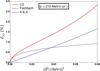
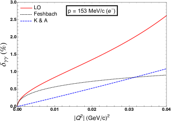
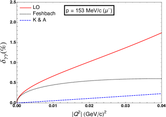
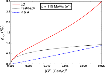
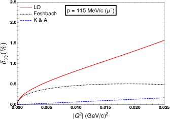
Figure 2: The fractional LO TPE contributions (expressed in percentage) to the elastic lepton-proton scattering cross-section [i.e., of ${\mathcal{O}}(\alpha)$] in HB$\chi$PT, Eq. (29). The left (right) panel displays the results for $e$-p ($\mu$-p) scattering versus the squared four-momentum transfer $|Q^{2}|$, for the MUSE beam momenta of $|\vec{p}\,|=p=115,\,153,\,210$ MeV/c. Each plot covers the full kinematical scattering range, $0<|Q^{2}|<|Q^{2}_{\rm max}|$ when $\theta\in[0,\pi]$. For comparison, the results for the well-known McKinley-Feshbach contribution, Eq. (30), (denoted as “Feshbach”), and that of Ref. Koshchii:2017dzr (denoted as “K & A”), are also displayed.

III.3 Next-to-leading order TPE corrections, i.e., ${\mathcal{O}}(\alpha/M)$

The NLO TPE fractional radiative corrections to elastic cross-section are of ${\mathcal{O}}(\alpha/M)$ contribution from each TPE diagram. As discussed earlier, they include both the ${\mathcal{O}}(1/M)$ parts of the TPE diagrams, (a) and (b), as well as the NLO chiral order TPE diagrams, (c) - (i), either with one proton-photon vertex stemming from the NLO Lagrangian ${\mathcal{L}}^{(1)}_{\pi N}$, Eq. (2), or with an insertion of an NLO proton propagator.

First, we display our result for the ${\mathcal{O}}(1/M)$ parts of the (a) plus (b) diagrams. This part is obtained by eliminating the true LO contributions $\delta^{\rm(0)}_{\gamma\gamma}$ from the complete contribution from (a) and (b) diagrams, $\delta^{\rm(ab)}_{\gamma\gamma}$. It is represented by the following expression:

$$\delta^{\rm(ab;\,1/M)}_{\gamma\gamma}(Q^{2})\! = \!\delta^{\rm(ab)}_{\gamma\gamma}(Q^{2})-\delta^{\rm(0)}_{\gamma\gamma}(Q^{2})=\delta^{(a)}_{\rm box}(Q^{2})+\delta^{(b)}_{\rm xbox}(Q^{2})-\left[\delta^{(a)}_{\rm box}(Q^{2})+\delta^{(b)}_{\rm xbox}(Q^{2})\right]_{\text{LO}}$$ (32)

$$= \!-\,16\pi\alpha E\,{\mathcal{R}}e\left[\delta^{(1/M)}I^{+}(p^{\prime},0|1,0,1,1)\right]+8\pi\alpha\frac{Q^{2}}{M}\,{\mathcal{R}}e\,\left[I^{(0)}(p,0|1,0,1,1)\right]$$

$$\!-\,16\pi\alpha E\,{\mathcal{R}}e\,\left[\delta^{(1/M)}I^{-}(p,0|0,1,1,1)+\delta^{(1/M)}I^{+}(p^{\prime},0|0,1,1,1)\right]$$

$$\!+\,4\pi\alpha\frac{Q^{2}}{M}\left[\frac{8E^{2}}{Q^{2}+4E^{2}}\right]\,{\mathcal{R}}e\,\left[I^{(0)}(p,0|0,1,1,1)\right]+8\pi\alpha\frac{Q^{2}}{M}\!\left[\frac{Q^{2}}{Q^{2}+4E^{2}}\right]\!\left[\frac{Q^{2}-4E^{2}}{Q^{2}+4E^{2}}\right]\!{\mathcal{R}}e\left[I(Q|1,1,0,1)\right]$$

$$\!-\,8\pi\alpha\frac{Q^{2}}{M}\left[\frac{Q^{2}+8E^{2}}{Q^{2}+4E^{2}}\right]\,{\mathcal{R}}e\,\left[Z^{(0)}(\Delta,i\sqrt{-Q^{2}}/2,m_{l},E)\right]$$

$$\!+\,16\pi\alpha E\left[\frac{Q^{2}+8E^{2}}{Q^{2}+4E^{2}}\right]\,{\mathcal{R}}e\,\left[\delta^{(1/M)}Z^{-}(\Delta,i\sqrt{-Q^{2}}/2,m_{l},E)+\delta^{(1/M)}Z^{+}(\Delta^{\prime},i\sqrt{-Q^{2}}/2,m_{l},-E^{\prime})\right]$$

$$\!+\,{\mathcal{O}}\left(M^{-2}\right)\,.$$

Here, the functions $I^{(0)}$ and $Z^{(0)}$ [cf. Eqs. (73) and (74)] denote the LO parts of the three-, and four-point functions $I^{-}$ and $Z^{-}$, respectively, as displayed in Appendix B. Also, $\delta^{(1/M)}I^{\pm}$ [cf. Eqs. (75) and (76)] and $\delta^{(1/M)}Z^{\pm}$ [cf. Eqs. (77) and (78)], denote the ${\mathcal{O}}(1/M)$ parts of the functions $I^{\pm}$ and $Z^{\pm}$, respectively. It is noteworthy that Eq. (32) is IR-singular due to the presence of the IR-divergent integrals $I^{-}(p,0|1,0,1,1)\equiv I^{(0)}(p,0|1,0,1,1)$ and $I^{+}(p^{\prime},0|1,0,1,1)$ [cf. Eqs. (61) and (62)]. The LO IR-divergent terms arising for these integrals, however, cancel each other leaving only ${\mathcal{O}}(1/M)$ residual IR divergences arising from terms containing the integral $I^{+}(p^{\prime},0|1,0,1,1)$. Thus, the resulting IR divergence from Eq. (32), extracted using dimensional regularization in $D=4-2\epsilon$ dimension, with pole $\epsilon<0$ and arbitrary renormalization scale $\mu$, has the form:

$$\delta^{\rm(box)}_{\rm IR}(Q^{2})\! \equiv \!\delta^{\rm(ab;\,1/M)}_{\gamma\gamma}(Q^{2})\Big{|}_{\rm IR}=-\,16\pi\alpha E\,{\mathcal{R}}e\left[\delta^{(1/M)}I^{+}(p^{\prime},0|1,0,1,1)\right]_{\rm IR}+8\pi\alpha\frac{Q^{2}}{M}\,{\mathcal{R}}e\,\left[I^{(0)}(p,0|1,0,1,1)\right]_{\rm IR}$$ (33)

$$= \!-\,\frac{\alpha Q^{2}}{2\pi ME\beta^{2}}\left[\frac{1}{\epsilon}-\gamma_{E}+\ln\left(\frac{4\pi\mu^{2}}{m_{l}^{2}}\right)\right]\left\{1+\left(\beta-\frac{1}{\beta}\right)\ln\sqrt{\frac{1+\beta}{1-\beta}}\,\right\}+{\mathcal{O}}\left(\frac{1}{M^{2}}\right)\,.$$

where $\gamma_{E}=0.577216...$ is the Euler-Mascheroni constant. The above NLO TPE contributions constitute the only IR-divergent terms $\delta^{\rm(box)}_{\rm IR}$ that arise in our calculations. These IR divergences exactly cancel with the soft-bremsstrahlung IR-divergent counterparts $\delta^{\rm(soft)}_{\rm IR}$ originating from the ${\mathcal{O}}(1/M)$ kinematical part of the interference contributions of the LO soft-bremsstrahlung radiation diagrams, such that, $\delta^{\rm(soft)}_{\rm IR}=-\delta^{\rm(box)}_{\rm IR}$. An explicit demonstration of this cancellation will be detailed in a future publication. We remark that in the IR divergent expression, Eq. (33), we include a constant term proportional to $\ln\left(\mu^{2}/m_{l}^{2}\right)$ whereas in Refs. Talukdar:2019dko ; Talukdar:2020aui ; Cao:2021nhm the corresponding IR divergence was written with a $Q^{2}$-dependent term proportional to $\ln\left(-Q^{2}/\mu^{2}\right)$. The difference produces a term proportional to $\ln\left(-Q^{2}/m_{l}^{2}\right)$ which affects the finite part of the TPE contribution markedly.

In Fig. 3, we present a comparison between the true LO TPE corrections $\delta^{(0)}_{\gamma\gamma}$ and the full TPE corrections arising from the (a) and (b) diagrams $\delta^{(a+b)}_{\gamma\gamma}$ which also include the proton propagator ${\mathcal{O}}(1/M)$ NLO contributions. As observed in this figure the NLO part of diagrams (a) and (b) in the electron-proton scattering case is negative and dominates over the positive true LO part. In contrast, for the muon-proton scattering the NLO parts of these diagrams are quite small and barely alter the LO results.

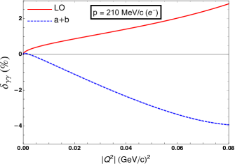
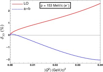
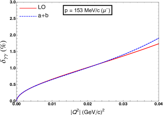
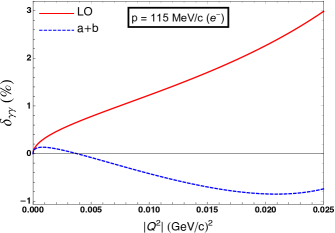
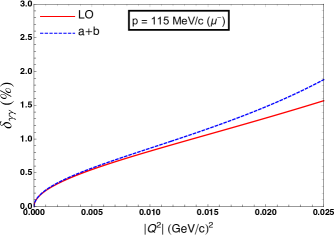
Figure 3: Comparison between the true LO TPE corrections $\delta^{(0)}_{\gamma\gamma}$ (denoted above as “LO”) and the full TPE corrections from the (a) and (b) diagrams $\delta^{(a+b)}_{\gamma\gamma}$ (denoted above as “a+b”) in HB$\chi$PT. The left (right) panel displays the results for e-p ($\mu$-p) scattering versus the squared four-momentum transfer $|Q^{2}|$, for the MUSE beam momenta of $|\vec{p}\,|=p=115,\,153,\,210$ MeV/c. Each plot covers the full kinematical scattering range, $0<|Q^{2}|<|Q^{2}_{\rm max}|$ with $\theta\in[0,\pi]$.

Next, we turn to the NLO chiral order diagrams (c) and (d), as well as (e) and (f), obtained by replacing one LO vertex with one NLO vertex, namely,

$$\delta^{(c)}_{\rm box}(Q^{2})\! = \!\frac{2{\mathcal{R}}e\sum\limits_{spins}\bigg{[}\mathcal{M}^{(0)*}_{\gamma}\widetilde{\mathcal{M}}^{(c)}_{\rm box}\bigg{]}}{\sum\limits_{spins}\left|\mathcal{M}^{(0)}_{\gamma}\right|^{2}}$$ (34)

$$= \!-\,\frac{2\pi\alpha}{M}\left[\frac{Q^{2}}{Q^{2}+4EE^{\prime}}\right]{\mathcal{R}}e\,\left\{\frac{1}{i}\int\frac{{\rm d}^{4}k}{{(2\pi)}^{4}}\frac{{\rm Tr}\left[(\not{p}+m_{l})\,\not{v}\,(\not{p}^{\,\prime}+m_{l})\,\not{v}\,(\not{p}-\not{k}+m_{l})\,\not{k}\right]}{(k^{2}+i0)\,\left[(Q-k)^{2}+i0\right]\,(k^{2}-2k\cdot p+i0)\,(v\cdot k+i0)}\right\}\,,$$

$$\delta^{(d)}_{\rm xbox}(Q^{2})\! = \!\frac{2{\mathcal{R}}e\sum\limits_{spins}\bigg{[}\mathcal{M}^{(0)*}_{\gamma}\widetilde{\mathcal{M}}^{(d)}_{\rm xbox}\bigg{]}}{\sum\limits_{spins}\left|\mathcal{M}^{(0)}_{\gamma}\right|^{2}}$$ (35)

$$= \!-\,\frac{2\pi\alpha}{M}\left[\frac{Q^{2}}{Q^{2}+4EE^{\prime}}\right]{\mathcal{R}}e\,\left\{\frac{1}{i}\int\frac{{\rm d}^{4}k}{{(2\pi)}^{4}}\frac{{\rm Tr}\left[(\not{p}+m_{l})\,\not{v}\,(\not{p}^{\,\prime}+m_{l})\,\not{k}\,(\not{p}+\not{k}-\not{Q}+m_{l})\,\not{v}\right]}{(k^{2}+i0)\,\left[(Q-k)^{2}+i0\right]\,(k^{2}+2k\cdot p^{\prime}+i0)\,(v\cdot k+i0)}\right\}\,,$$

$$\delta^{(e)}_{\rm box}(Q^{2})\! = \!\frac{2{\mathcal{R}}e\sum\limits_{spins}\bigg{[}\mathcal{M}^{(0)*}_{\gamma}\widetilde{\mathcal{M}}^{(e)}_{\rm box}\bigg{]}}{\sum\limits_{spins}\left|\mathcal{M}^{(0)}_{\gamma}\right|^{2}}$$ (36)

$$= \!-\,\frac{2\pi\alpha}{M}\left[\frac{Q^{2}}{Q^{2}+4EE^{\prime}}\right]{\mathcal{R}}e\,\left\{\frac{1}{i}\int\frac{{\rm d}^{4}k}{{(2\pi)}^{4}}\frac{{\rm Tr}\left[(\not{p}+m_{l})\,\not{v}\,(\not{p}^{\,\prime}+m_{l})\,(\not{k}+\not{Q})\,(\not{p}-\not{k}+m_{l})\,\not{v}\right]}{(k^{2}+i0)\,\left[(Q-k)^{2}+i0\right]\,(k^{2}-2k\cdot p+i0)\,(v\cdot k+i0)}\right\}\,,$$

and

$$\delta^{(f)}_{\rm xbox}(Q^{2})\! = \!\frac{2{\mathcal{R}}e\sum\limits_{spins}\bigg{[}\mathcal{M}^{(0)*}_{\gamma}\widetilde{\mathcal{M}}^{(f)}_{\rm xbox}\bigg{]}}{\sum\limits_{spins}\left|\mathcal{M}^{(0)}_{\gamma}\right|^{2}}$$ (37)

$$= \!-\,\frac{2\pi\alpha}{M}\left[\frac{Q^{2}}{Q^{2}+4EE^{\prime}}\right]{\mathcal{R}}e\,\left\{\frac{1}{i}\int\frac{{\rm d}^{4}k}{{(2\pi)}^{4}}\frac{{\rm Tr}\left[(\not{p}+m_{l})\,\not{v}\,(\not{p}^{\,\prime}+m_{l})\,\not{v}\,(\not{p}+\not{k}-\not{Q}+m_{l})\,(\not{k}+\not{Q})\right]}{(k^{2}+i0)\,\left[(Q-k)^{2}+i0\right]\,(k^{2}+2k\cdot p^{\prime}+i0)\,(v\cdot k+i0)}\right\}\,.$$

These TPE diagrams also have higher-order contributions that we neglect in our NLO evaluations. Using IBP methods the contributions from the (c) and (d) diagrams can be expressed in terms of the real part of the IR-finite three-point integral $I(Q|1,1,0,1)$ given in Eq.(27) [also see Eq. (85)]:

$$\delta^{(c)}_{\rm box}(Q^{2})\! = \!4\pi\alpha\frac{Q^{2}}{M}\,{\mathcal{R}}e\,\left[I(Q|1,1,0,1)\right]\,,\quad\text{and}$$ (38)

$$\delta^{(d)}_{\rm xbox}(Q^{2})\! = \!-\,4\pi\alpha\frac{Q^{2}}{M}\,{\mathcal{R}}e\,\left[I(Q|1,1,0,1)\right]\,,$$ (39)

which means that their sum is

$$\delta^{(c+d)}_{\gamma\gamma}(Q^{2})=\delta^{(c)}_{\rm box}(Q^{2})+\delta^{(d)}_{\rm xbox}(Q^{2})=0\,.$$ (40)

Thus, the net contribution from the (c) and (d) diagrams to the TPE radiative corrections vanishes. The other two diagrams, namely, (e) and (f) diagrams are given by the following expressions:

$$\delta^{(e)}_{\rm box}(Q^{2})\! = \!-\,\frac{4\pi\alpha}{M}\left[\frac{Q^{2}}{Q^{2}+4EE^{\prime}}\right]{\mathcal{R}}e\,\bigg{\{}\!-2(Q^{2}+2E^{2})\,I^{-}(p,0|0,1,1,1)+4E^{2}\,I^{-}(p,0|1,0,1,1)+(Q^{2}-4E^{2})$$ (41)

$$\hskip 113.81102pt\times\,I(Q|1,1,0,1)+4EQ^{2}\,I^{-}(p,0|1,1,1,0)-4E^{2}Q^{2}\,I^{-}(p,0|1,1,1,1)\bigg{\}}$$

$$= \!-\,\frac{4\pi\alpha}{M}\left[\frac{Q^{2}}{Q^{2}+4E^{2}}\right]{\mathcal{R}}e\,\bigg{\{}\!-2(Q^{2}+4E^{2})\,I^{(0)}(p,0|0,1,1,1)+(Q^{2}-4E^{2})\,I(Q|1,1,0,1)$$

$$\hskip 110.96556pt+\,4EQ^{2}\,I(Q|1,1,1,0)+8E^{2}\,Z^{(0)}(\Delta,i\sqrt{-Q^{2}}/2,m_{l},E)\bigg{\}}+{\mathcal{O}}\left(\frac{1}{M^{2}}\right)\,,\quad\,\,$$

and

$$\delta^{(f)}_{\rm xbox}(Q^{2})\! = \!-\,\frac{4\pi\alpha}{M}\left[\frac{Q^{2}}{Q^{2}+4EE^{\prime}}\right]{\mathcal{R}}e\,\bigg{\{}2(Q^{2}+2E^{2})\,I^{+}(p^{\prime},0|0,1,1,1)-4E^{2}\,I^{+}(p^{\prime},0|1,0,1,1)-(Q^{2}-4E^{2})$$ (42)

$$\hskip 113.81102pt\times\,I(Q|1,1,0,1)+4EQ^{2}\,I^{+}(p^{\prime},0|1,1,1,0)+4E^{2}Q^{2}\,I^{+}(p^{\prime},0|1,1,1,1)\bigg{\}}$$

$$= \!-\,\frac{4\pi\alpha}{M}\left[\frac{Q^{2}}{Q^{2}+4E^{2}}\right]{\mathcal{R}}e\,\bigg{\{}\!-2(Q^{2}+4E^{2})\,I^{(0)}(p,0|0,1,1,1)-(Q^{2}-4E^{2})\,I(Q|1,1,0,1)$$

$$\hskip 110.96556pt+\,4EQ^{2}\,I(Q|1,1,1,0)+8E^{2}\,Z^{(0)}(\Delta,i\sqrt{-Q^{2}}/2,m_{l},E)\bigg{\}}+{\mathcal{O}}\left(\frac{1}{M^{2}}\right)\,.\quad\,\,$$

The IR-finite three-point integrals, $I(Q|1,1,1,0)\equiv I^{-}(p,0|1,1,1,0)\equiv I^{+}(p^{\prime},0|1,1,1,0)$, are purely relativistic and depend only on the momentum transfer $Q^{2}$ [cf. Eq. (86)]. It is important to note that the IR-divergent functions, namely, $I^{-}(p,0|1,0,1,1)$ and $I^{+}(p^{\prime},0|1,0,1,1)$ [arising due to the decompositions, Eq. (25)], drop out from the above expressions leading to IR-finite contributions from each of (e) and (f) NLO diagrams. Thus, the net contribution to the TPE radiative corrections from the (e) and (f) diagrams is finite and displayed in Fig. 4. Notably, the sizable corrections in the case of electron-proton scattering arise primarily due to the dominance of the integral $I(Q|1,1,1,0)$ at large $Q^{2}$ values.

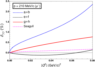
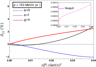
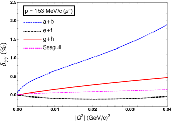
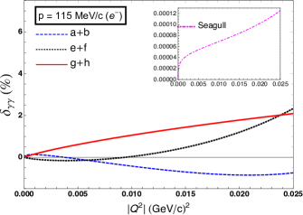
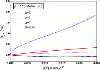
Figure 4: Various diagrammatic contributions to the TPE radiative corrections to the elastic cross-section. The pair-wise contributions from the TPE diagrams, namely, (a) + (b), (e) + (f), and (g) + (h) are displayed, along with that of the seagull diagram (i). The left (right) panel displays the results for e-p ($\mu$-p) scattering versus the squared four-momentum transfer $|Q^{2}|$, for the MUSE beam momenta of $|\vec{p}\,|=p=115,\,153,\,210$ MeV/c. Each plot covers the full kinematical scattering range, $0<|Q^{2}|<|Q^{2}_{\rm max}|$ with $\theta\in[0,\pi]$. The seagull contribution for the electron scattering is tiny and is displayed in the inset plots.

Next, we display our analytical results for the (g) and (h) NLO diagrams containing the NLO proton propagator insertions, where we employ Eqs. (52) and (53), namely,

$$\delta^{(g)}_{\rm box}(Q^{2})\! = \!\frac{2{\mathcal{R}}e\sum\limits_{spins}\bigg{[}\mathcal{M}^{(0)*}_{\gamma}\widetilde{\mathcal{M}}^{(g)}_{\rm box}\bigg{]}}{\sum\limits_{spins}\left|\mathcal{M}^{(0)}_{\gamma}\right|^{2}}$$ (43)

$$= \!\frac{2\pi\alpha}{M}\left[\frac{Q^{2}}{Q^{2}+4EE^{\prime}}\right]{\mathcal{R}}e\,\left\{\frac{1}{i}\int\frac{{\rm d}^{4}k}{{(2\pi)}^{4}}\frac{{\rm Tr}[(\not{p}+m_{l})\,\not{\!v}\,(\not{p}^{\,\prime}+m_{l})\,\not{v}\,(\not{p}-\not{k}+m_{l})\,\not{v}]}{\left[(Q-k)^{2}+i0\right]\,(k^{2}-2k\cdot p+i0)\,(v\cdot k+i0)^{2}}\right\}$$

$$= \!-\,\frac{4\pi\alpha}{M}\left[\frac{Q^{2}}{Q^{2}+4EE^{\prime}}\right]{\mathcal{R}}e\,\bigg{\{}(Q^{2}+8E^{2})\,I^{-}(p,0|0,1,1,1)-2E(Q^{2}+4E^{2})\,I^{-}(p,0|0,1,1,2)$$

$$\hskip 113.81102pt-\,2(E^{\prime}p+Ep^{\prime})\cdot I^{-}_{1}(p,0|0,1,1,2)\bigg{\}}$$

$$= \!-\frac{4\pi\alpha}{M}\left[\frac{Q^{2}}{Q^{2}+4E^{2}}\right]{\mathcal{R}}e\,\bigg{\{}(Q^{2}+8E^{2})\,I^{(0)}(p,0|0,1,1,1)-E\left(Q^{2}+8E^{2}+4m^{2}_{l}\right)\,I^{(0)}(p,0|0,1,1,2)$$

$$\hskip 105.2751pt-\,2\left[(E^{\prime}p+Ep^{\prime})\cdot T^{-}_{1}(p,0|0,1,1,2)\right]_{\rm LO}\bigg{\}}+{\mathcal{O}}\left(\frac{1}{M^{2}}\right)\,,$$

and

$$\delta^{(h)}_{\rm xbox}(Q^{2})\! = \!\frac{2{\mathcal{R}}e\sum\limits_{spins}\bigg{[}\mathcal{M}^{(0)}_{\gamma}\widetilde{\mathcal{M}}^{(h)}_{\rm xbox}\bigg{]}}{\sum\limits_{spins}\left|\mathcal{M}^{(0)}_{\gamma}\right|^{2}}$$ (44)

$$= \!\frac{2\pi\alpha}{M}\left[\frac{Q^{2}}{Q^{2}+4EE^{\prime}}\right]{\mathcal{R}}e\left\{\frac{1}{i}\int\frac{{\rm d}^{4}k}{{(2\pi)}^{4}}\frac{{\rm Tr}[(\not{p}+m_{l})\,\not{v}\,(\not{p}^{\,\prime}+m_{l})\,\not{v}\,(\not{p}+\not{k}-\not{Q}+m_{l})\,\not{\!v}]}{\left[(Q-k)^{2}+i0\right]\,(k^{2}+2k\cdot p^{\prime}+i0)\,(v\cdot k+i0)^{2}}\right\}$$

$$= \!-\,\frac{4\pi\alpha}{M}\left[\frac{Q^{2}}{Q^{2}+4EE^{\prime}}\right]{\mathcal{R}}e\,\bigg{\{}\!-(Q^{2}+8E^{2})\,I^{+}(p^{\prime},0|0,1,1,1)-2E(Q^{2}+4E^{2})\,I^{+}(p^{\prime},0|0,1,1,2)$$

$$\hskip 113.81102pt+\,2(E^{\prime}p+Ep^{\prime})\cdot I^{+}_{1}(p^{\prime},0|0,1,1,2)\bigg{\}}$$

$$= \!-\frac{4\pi\alpha}{M}\left[\frac{Q^{2}}{Q^{2}+4E^{2}}\right]{\mathcal{R}}e\,\bigg{\{}(Q^{2}+8E^{2})\,I^{(0)}(p,0|0,1,1,1)+E\left(Q^{2}+8E^{2}+4m^{2}_{l}\right)\,I^{(0)}(p,0|0,1,1,2)$$

$$\hskip 113.81102pt+\,2\left[(E^{\prime}p+Ep^{\prime})\cdot T^{+}_{1}(p^{\prime},0|0,1,1,2)\right]_{\rm LO}\bigg{\}}$$

$$\!-\,\frac{\alpha Q^{2}}{2\pi ME\beta^{3}}\left[\frac{Q^{2}+8E^{2}+4m^{2}_{l}}{Q^{2}+4E^{2}}\right]\left\{\ln\sqrt{\frac{1+\beta}{1-\beta}}-\beta\right\}+{\mathcal{O}}\left(\frac{1}{M^{2}}\right)\,,$$

respectively, The above functions, $I^{-\mu}_{1}(p,0|0,1,1,2)$ and $I^{+\mu}_{1}(p^{\prime},0|0,1,1,2)$ [or alternatively, $T^{-\mu}_{1}(p,0|0,1,1,2)$ and $T^{+\mu}_{1}(p^{\prime},0|0,1,1,2)$], are rank-1 tensor integrals containing a single power of the loop momentum $k^{\mu}$ [or alternatively, $(k-p)^{\mu}$ and $(k+p^{\prime})^{\mu}$] in the numerators, Eqs. (51) and  (53). The symbol $[...]_{\rm LO}$ in the above expressions denotes LO terms to be considered within braces. We should note that when we add the (g) and (h) contributions from Eqs. (43) and (44), the integral $I^{(0)}(p,0|0,1,1,2)$ cancels. Furthermore, only the difference, $T_{1}^{-}-T_{1}^{+}$, is relevant when considering the sum of (g) and (h) diagrams. The above integrals are evaluated by decomposing into simple scalar master integrals via the standard technique of Passarino-Veltman reduction Passarino:1979 (PV). To this end, we can decompose the tensor structures of $T^{\pm\,\mu}_{1}$ in terms of three independent external four-vectors, e.g., $v$, $p$ and $p^{\prime}$:

$$T^{-\mu}_{1}(p,0|0,1,1,2)\! = \!v^{\mu}C^{-}_{1}+p^{\prime\,\mu}C^{-}_{2}\,,$$

$$T^{+\mu}_{1}(p^{\prime},0|0,1,1,2)\! = \!v^{\mu}C^{+}_{1}+p^{\mu}C^{+}_{2}\,.$$ (45)

The coefficients, $C^{\pm}_{1,2}=\,\stackrel{{\scriptstyle\circ}}{{C^{\pm}_{1,2}}}+{\mathcal{O}}(1/M)$, are combinations of scalar master integrals, as discussed in Appendix B. Only the LO parts of $C^{\pm}_{1,2}$ (as obtained by replacing $E^{\prime}=E$ and $\beta^{\prime}=\beta$) are relevant in our context, namely,

$$\stackrel{{\scriptstyle\circ}}{{C^{-}_{1}}}\! = \!\left[1-\frac{1}{\beta^{2}}\right]I^{(0)}(p,0|0,1,1,1)+\frac{1}{2E\beta^{2}}\left[I^{(0)}(p,0|0,0,1,2)-I(Q|0,1,0,2)\right]\,,$$

$$\stackrel{{\scriptstyle\circ}}{{C^{-}_{2}}}\! = \!\frac{1}{E\beta^{2}}I^{(0)}(p,0|0,1,1,1)-I^{(0)}(p,0|0,1,1,2)-\frac{1}{2E^{2}\beta^{2}}\left[I^{(0)}(p,0|0,0,1,2)-I(Q|0,1,0,2)\right]\,,$$

$$\stackrel{{\scriptstyle\circ}}{{C^{+}_{1}}}\! = \!-\,\left[1-\frac{1}{\beta^{2}}\right]I^{(0)}(p,0|0,1,1,1)-\frac{1}{2E\beta^{2}}\left[I^{(0)}(p,0|0,0,1,2)-I(Q|0,1,0,2)\right]\,,\quad\text{and}$$

$$\stackrel{{\scriptstyle\circ}}{{C^{+}_{2}}}\! = \!-\,\frac{1}{E\beta^{2}}I^{(0)}(p,0|0,1,1,1)-I^{(0)}(p,0|0,1,1,2)+\frac{1}{2E^{2}\beta^{2}}\left[I^{(0)}(p,0|0,0,1,2)-I(Q|0,1,0,2)\right]$$ (46)

$$\!-\,\frac{2}{(4\pi)^{2}E^{2}\beta^{3}}\left[\ln\sqrt{\frac{1+\beta}{1-\beta}}-\beta\right]\,.$$

In particular, the two-point functions, $I^{(0)}(p,0|0,0,1,2)$ and $I(Q|0,1,0,2)$, appear as a difference in our chiral order. Therefore, their UV divergences cancel exactly as they should since we only take the difference of these integrals in each of the above coefficients $\stackrel{{\scriptstyle\circ}}{{C^{\pm}_{1,2}}}$, see Eq. (46) or Eq. (84):

$$I^{(0)}(p,0|0,0,1,2)-I(Q|0,1,0,2)$$

$$\hskip 28.45274pt=\,\frac{1}{8\pi^{2}}\left[\frac{2}{\beta}\ln\sqrt{\frac{1+\beta}{1-\beta}}+\ln\left(\frac{M^{2}m_{l}^{2}}{Q^{4}}\right)\,\,\right]\,.\qquad\,$$ (47)

All our results for the TPE radiative corrections are UV-finite, as expected from naive dimensional arguments. We observe that the presence of the lepton mass-dependent logarithmic term $\propto\ln\left(\frac{M^{2}m_{l}^{2}}{Q^{4}}\right)$ of Eq. (47), originating from the (g) and (h) diagrams, enhance the contributions for the electron scattering as compared to muon scattering. (see Fig. 4).

Furthermore, it is important to note that the three-point function $I^{(0)}(p,0|0,1,1,2)$ appearing in the individual contributions from the (g) and (h) diagrams, $\delta^{(g)}_{\rm box}$ and $\delta^{(h)}_{\rm xbox}$, is linear in the proton’s mass $M$ [cf. Eqs. (79)], and therefore, may lead to pathologies with the convergence of the chiral expansion. However, as noted, this integral appearing in both $\delta^{(g)}_{\rm box}$ and $\delta^{(g)}_{\rm xbox}$ cancel in the sum. Our combined result for the fractional contribution from the (g) and (h) diagrams become

$$\delta^{(gh)}_{\gamma\gamma}(Q^{2})\! = \!\delta^{(g)}_{\rm box}(Q^{2})+\delta^{(h)}_{\rm xbox}(Q^{2})$$ (48)

$$= \!-\,\frac{4\pi\alpha}{M}\left[\frac{Q^{2}}{Q^{2}+4E^{2}}\right]{\mathcal{R}}e\,\Bigg{\{}2\left[Q^{2}\left(1+\frac{1}{\beta^{2}}\right)+8E^{2}\right]I^{(0)}(p,0|0,1,1,1)$$

$$\hskip 108.12054pt-\,\left(\frac{Q^{2}+4E^{2}\beta^{2}}{E\beta^{2}}\right)\left[I^{(0)}(p,0|0,0,1,2)-I(Q|0,1,0,2)\right]\Bigg{\}}$$

$$\!-\,\frac{\alpha Q^{2}}{\pi ME\beta^{3}}\left[\ln\sqrt{\frac{1+\beta}{1-\beta}}-\beta\right]+{\mathcal{O}}\left(\frac{1}{M^{2}}\right)\,.$$

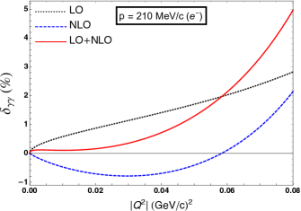
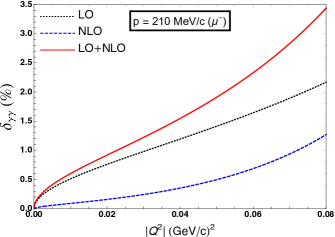
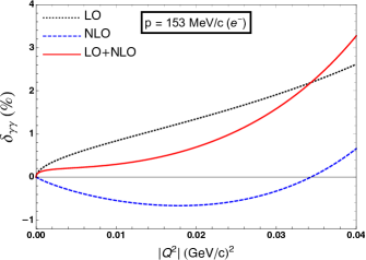
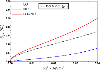
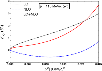
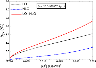
Figure 5: The fractional TPE contributions (expressed in percentage) to the elastic lepton-proton scattering cross-section [i.e., of ${\mathcal{O}}(\alpha)$] in HB$\chi$PT. Left (right) plots show TPE contribution for e-p ($\mu$-p) scattering, respectively, at specific MUSE beam momenta. Each plot covers the full kinematical scattering range, $0<|Q^{2}|<|Q^{2}_{\rm max}|$ with $\theta\in[0,\pi]$. The dotted (black) lines correspond to LO results, the dashed (blue) lines correspond to NLO corrections, while the thick solid (red) lines denote the total (LO plus NLO) contributions from all the TPE diagrams displayed in Fig. 1.

Finally, the least important NLO contribution to the TPE radiative corrections arises from the seagull diagram (i), without an elastic proton intermediate state. After initial cancellations, only the residual part $\widetilde{\mathcal{M}}^{(i)}_{\rm seagull}$ [see Eq. (16)] proportional to $g^{\mu\nu}$ contributes to the NLO cross-section:

$$\delta^{\rm(seagull)}_{\gamma\gamma}(Q^{2})\! = \!\frac{2{\mathcal{R}}e\,\sum_{spins}\bigg{[}{\mathcal{M}}^{(0)*}_{\gamma}\,\widetilde{\mathcal{M}}^{(i)}_{\rm seagull}\bigg{]}}{\sum_{spin}\left|{\mathcal{M}}^{(0)}_{\gamma}\right|^{2}}$$

$$= \!\frac{4\pi\alpha}{M}\left[\frac{Q^{2}}{Q^{2}+4EE^{\prime}}\right]{\mathcal{R}}e\,\left\{\frac{1}{i}\int\frac{{\rm d}^{4}k}{{(2\pi)}^{4}}\frac{{\rm Tr}[(\not{\!p}+m_{l})\,\gamma^{\rho}\,(\not{\!p^{\prime}}+m_{l})\,\gamma^{\mu}\,(\not{\!p}-\not{\!k}+m_{l})\,\gamma_{\mu}\,v_{\rho}]}{(k^{2}+i0)\,\left[(Q-k)^{2}+i0\right]\,(k^{2}-2k\cdot p+i0)}\right\}$$

$$= \,\frac{4\pi\alpha}{M}\left\{\frac{Q^{2}}{Q^{2}+4EE^{\prime}}\right]{\mathcal{R}}e\,\bigg{\{}4\left(Q^{2}v+2Ep+2Ep^{\prime}\right)\cdot I^{-}_{1}(p,0|1,1,1,0)+16m_{l}^{2}E\,I(Q|1,1,1,0)\bigg{\}}$$

$$= \!-\frac{4\alpha E}{\pi M}\left[\frac{Q^{2}}{Q^{2}+4E^{2}}\right]{\mathcal{R}}e\,\bigg{\{}\left(\frac{1-\nu^{2}}{2\nu^{2}}\right)\ln\left(\frac{-Q^{2}}{m^{2}_{l}}\right)-(4\pi)^{2}m_{l}^{2}\left(\frac{1+\nu^{2}}{\nu^{2}}\right)I(Q|1,1,1,0)\bigg{\}}+{\mathcal{O}}\left(\frac{1}{M^{2}}\right)\,,$$ (49)

where $\nu=\sqrt{1-4m^{2}_{l}/Q^{2}}$ is a $Q^{2}$-dependent kinematical variable. The analytical results for the relativistic three-point scalar $I(Q|1,1,1,0)$ and tensor $I^{-\mu}_{1}(p,0|1,1,1,0)$ integrals are expressed in Eqs. (86) and (87). In the case of muon scattering, the second term in the seagull contribution being proportional to the square of its mass leads to some enhancements in the result as compared to the electron case, where the contribution is tiny (see Fig. 4). For a detailed discussion about the seagull contribution, we refer the reader to Ref. Talukdar:2019dko .

IV Results and discussion

In Figs. 2 - 5, we provide the numerical results of our analytically derived expressions for the box, crossed-box, and seagull TPE contributions, after removal of the IR-divergent terms [see Eq. (33)]. In Fig. 2 our LO correction results, Eq. (29), are plotted for e-p and $\mu$-p scatterings, at the three specific MUSE choices of the incoming lepton momenta. In the same figure, we also compared our results to other TPE works, e.g., Ref. Koshchii:2017dzr , based on relativistic QED invoking SPA Tsai:1961zz , as well as the well-known estimate, Eq. (30) of McKinley and Feshbach McKinley:1948zz , based on the scattering of relativistic electrons off static Coulomb potentials in the context of the second Born approximation.

Our final results of evaluating the TPE radiative corrections to the elastic cross-sections are consolidated in Fig. 5, where we present a comparison of LO versus NLO contribution from HB$\chi$PT. As seen from the figure [see also Fig. 3], for e-p scattering the HB$\chi$PT expansion does not appear to be reliable. In the figures, LO corresponds to the true LO result which stems from diagrams (a) and (b), Eq. (29). In addition, as we have discussed earlier, the diagrams (a) and (b) also contain NLO contributions from Eq. (32) that for the case of e-p scattering are dominating the positive LO part. In fact, these NLO contributions from the (a) and (b) diagrams make the total NLO corrections from all TPE diagrams, (a) - (i) in Fig. 1 negative for the most part of the $Q^{2}$ domain, as shown in the left panel plots of Fig. 5. However, in a forthcoming publication, we shall demonstrate that our NLO results diminish when we consider the contributions of the finite part of the corresponding soft-bremsstrahlung diagrams. We shall show that the source of this change in our results can be attributed to the “large” ${\rm ln}\left(-Q^{2}/m_{l}^{2}\right)$ which appears in the soft-bremsstrahlung process. In contrast, for muon-proton scattering with $Q^{2}\sim m^{2}_{\mu}$, the above ”log”-factor is very small and will not markedly affect the HB$\chi$PT perturbative expansion. Another observation concerns the NLO propagator insertion diagrams, (g) and (h), whose contributions are almost as large as the LO contribution for e-p scattering. The former corrections have a positive sign and they diminish the negative NLO corrections from (a) and (b) diagrams, which also include $1/M$ order correction terms to the proton propagator. We further observe that the box diagram (c) exactly cancels the contribution from the crossed-box (d) diagram, see below Eq. (40). Finally, we find from Fig. 5 that for e-p scattering the two IR-finite diagrams, (e) and (f), become large for $Q^{2}\gtrsim 0.02$ (GeV/c)², especially due to the contribution of the relativistic three-point integral $I(Q|1,1,1,0)$. In this context, we note that even at the kinematic regime relevant to the MUSE, the electron is relativistic. However, the muon being much heavier is not expected to behave as a true relativistic probe in this regime.

Turning to muon-proton scattering results we find significant differences in the TPE corrections compared to the electron-proton scattering results. For the $\mu$-p scattering case, the LO contribution dominates the NLO contribution in the entire MUSE kinematical domain. Furthermore, both LO and NLO contributions are positive in the whole $Q^{2}$ range. These results indicate that the perturbative aspects of HB$\chi$PT appear to behave more robustly for $\mu$-p scattering. In particular, we find from Fig. 4 (right panel) that the contributions from the NLO TPE diagrams (g) and (h) are significantly smaller than that of the LO, which sharply contrasts the corresponding e-p scattering results (left panel). Nonetheless, their contributions are the most significant ones among all other NLO corrections. Another contrasting feature regarding the muon results is the following: while on the one hand, the (e) and (f) diagrams have rather small contributions in this case, the role of the seagull diagram, on the other hand, becomes quite relevant, see Fig. 4. Finally, we observe that the total TPE correction including the NLO contributions to $\mu$-p scattering is somewhat smaller than the size of e-p scattering.

We can clearly see the impact of our exact analytical results in comparison to the SPA results of Ref. Talukdar:2019dko also in the context of HB$\chi$PT. There the calculation applied SPA both in the numerator and denominator of the lepton propagators which appear in the TPE box and crossed-box diagrams. The results in that work were expressed solely in terms of the IR-divergent three-point functions, $I^{-}(p,0|1,0,1,1)$ and $I^{+}(p^{\prime},0|1,0,1,1)$. The application of SPA is in effect tantamount to suppressing the effects arising from several such integrals which potentially yield sizeable numerical contributions, as evidenced in Figs. 4 and 5. For instance, the (e), (f), (g), and (h) diagram contributions would be greatly diminished in SPA by the absence of integrals, such as the three-point function, $I(Q|1,1,1,0)$, and to some extent the four-point function, $Z^{\pm}$. The most significant difference in the SPA results compared with our exact result is, however, the vanishing true LO contribution from diagrams (a) and (b) as obtained in Ref. Talukdar:2019dko . In other words, Ref. Talukdar:2019dko completely missed out on the Feshbach contribution, Eq. (30) McKinley:1948zz . In contrast, our current results in Fig. 2 suggest that the LO contribution to TPE radiative corrections exceeds $2\%$ at the largest $Q^{2}$ values, essentially stemming from the integral $I(Q|1,1,0,1)$ which is absent in a SPA evaluation. Nevertheless, a notable feature of the TPE radiative corrections is that at $Q^{2}=0$ these contributions identically vanish in all the different approaches/approximations.

V Summary and conclusion

We have presented in this work an exact analytical evaluation of LO and NLO contributions from two-photon exchange to the lepton-proton elastic unpolarized cross-section at low-energies in HB$\chi$PT, taking nonzero lepton mass into account. We find sizeable contributions beyond the expected SPA results, akin to the ones found via dispersion techniques, e.g., Ref. Tomalak:2014sva . Our EFT method contrasts several prior TPE analyses utilizing relativistic hadronic models, which frequently parameterize the proton-photon vertices using phenomenological form factors. It is notable that as per the tenets of HB$\chi$PT power counting, the proton is a point particle at order $1/M$. The proton structure effects, e.g., anomalous magnetic moment and pion-loop contributions, only start appearing at order $1/M^{2}$. Although such NNLO effects will also appear in the usual Born differential cross-section $\left[{\rm d}\sigma_{el}(Q^{2})/{\rm d}\Omega^{\prime}_{l}\right]_{\gamma}$, their influence on the fractional TPE radiative corrections $\delta^{\rm(box)}_{\gamma\gamma}$ are certainly sub-dominant. In fact, Ref. Kaiser:2010zz has done an exact e-$\mu$ TPE scattering calculation in the context of standard relativistic QED. Using the e-$\mu$ result of Ref. Kaiser:2010zz , in principle, one can replace the muon mass with the proton mass $M$ and make an expansion in $1/M$ and find our HB$\chi$PT $1/M$ results. However, such a calculation requires a nontrivial $1/M$ expansion which we have not performed in this work. The paper solely deals with the exact NLO estimation of the TPE radiative corrections without proton’s form factors modification in a non-systematic manner (although it is well-known that form factors reduce the overall magnitude of the TPE corrections). Nevertheless, a systematic NNLO calculation of the TPE should be pursued as our future endeavor. The major difference with the SPA evaluation of Ref. Talukdar:2019dko is that our calculations are done exactly including all soft- and hard-photon exchange configurations of the TPE loops. In fact, our current results are expected to exhibit sizeable differences with any existing SPA calculation using a perturbative/diagrammatic approach. Regarding the isolation of the IR divergences, we used dimensional regularization. They arise from the three-point functions, $I^{-}(p,0|1,0,1,1)$ and $I^{+}(p^{\prime},0|1,0,1,1)$ stemming only from diagrams (a) and (b). The remaining TPE diagrams have all finite contributions. Such an IR singular structure of our TPE results agrees with the recent evaluation base of manifestly Lorentz-invariant B$\chi$PT Cao:2021nhm . In our HB$\chi$PT approach, the IR singularities appearing at LO automatically drop out of the calculation with only residual NLO IR-singular terms remaining and they cancel against the relevant soft-bremsstrahlung IR-singular contributions at NLO.

Appendix A Notations

In this section, we present the notations for all the Feynman loop integrals used in this work. First, we start by presenting the following generic forms of the one-loop scalar master integrals with external four-momenta $p$ and $p^{\prime}$, four-momentum transfer $Q_{\mu}=(p-p^{\prime})_{\mu}$, and loop four-momentum $k_{\mu}$, having indices $n_{1,2,3,4}\in{\mathbb{Z}}_{\pm}$ and a real-valued parameter $\omega$:

$$I^{-}(p,\omega|n_{1},n_{2},n_{3},n_{4})\! = \!\frac{1}{i}\int\frac{{\rm d}^{4}k}{{(2\pi)}^{4}}\frac{1}{(k^{2}+i0)^{n1}\,[(k-Q)^{2}+i0]^{n2}\,(k^{2}-2k\cdot p+i0)^{n_{3}}\,(v\cdot k+\omega+i0)^{n4}}\,,$$

$$I^{+}(p^{\prime},\omega|n_{1},n_{2},n_{3},n_{4})\! = \!\frac{1}{i}\int\frac{{\rm d}^{4}k}{{(2\pi)}^{4}}\frac{1}{(k^{2}+i0)^{n1}\,[(k-Q)^{2}+i0]^{n2}\,(k^{2}+2k\cdot p^{\prime}+i0)^{n_{3}}\,(v\cdot k+\omega+i0)^{n4}}\,,$$

$$Z^{-}(\Delta,i\sqrt{-Q^{2}}/2,m_{l},\omega)\! = \!\frac{1}{i}\int\frac{{\rm d}^{4}k}{(2\pi)^{4}}\frac{1}{\left[(k+\Delta)^{2}-\frac{1}{4}Q^{2}+i0\right]\,(k^{2}-m^{2}_{l}+i0)\,\left(v\cdot k+\omega+i0\right)}\,,\quad\text{and}$$

$$Z^{+}(\Delta^{\prime},i\sqrt{-Q^{2}}/2,m_{l},\omega)\! = \!\frac{1}{i}\int\frac{{\rm d}^{4}k}{(2\pi)^{4}}\frac{1}{\left[(k+\Delta^{\prime})^{2}-\frac{1}{4}Q^{2}+i0\right]\,(k^{2}-m^{2}_{l}+i0)\,\left(v\cdot k+\omega+i0\right)}\,,$$ (50)

where the $Z^{\pm}$ integrals are functions of the additional four vectors, $\Delta_{\mu}=\left(p-\frac{Q}{2}\right)_{\mu}$ and $\Delta^{\prime}_{\mu}=-\left(p^{\prime}+\frac{Q}{2}\right)_{\mu}=-\left(p-\frac{Q}{2}\right)_{\mu}=-\Delta_{\mu}$. The parameter $\omega$ can be either zero, $\omega=v\cdot Q=-\frac{Q^{2}}{2M}$, or any finite quantity (e.g., $\omega=v\cdot p=E\,,\,\,-v\cdot p^{\prime}=-E^{\prime}$), depending on the specific integrals we are dealing with.

Next, we have the two tensor integrals with one power of the loop momentum in the numerators appearing in our work. They have the following generic forms:

$$I^{-\mu}_{1}(p,\omega|n_{1},n_{2},n_{3},n_{4})\! = \!\frac{1}{i}\int\frac{{\rm d}^{4}k}{{(2\pi)}^{4}}\frac{k^{\mu}}{(k^{2}+i0)^{n1}\,[(k-Q)^{2}+i0]^{n2}\,(k^{2}-2k\cdot p+i0)^{n_{3}}\,(v\cdot k+\omega+i0)^{n4}}\,,\quad\text{and}$$

$$I^{+\mu}_{1}(p^{\prime},\omega|n_{1},n_{2},n_{3},n_{4})\! = \!\frac{1}{i}\int\frac{{\rm d}^{4}k}{{(2\pi)}^{4}}\frac{k^{\mu}}{(k^{2}+i0)^{n1}\,[(k-Q)^{2}+i0]^{n2}\,(k^{2}+2k\cdot p^{\prime}+i0)^{n_{3}}\,(v\cdot k+\omega+i0)^{n4}}\,.$$ (51)

In particular, using the following transformations on the tensor integrals, $I^{-\mu}_{1}(p,0|0,1,1,2)$ and $I^{+\mu}_{1}(p^{\prime},0|0,1,1,2)$, used in this work:

$$2(E^{\prime}p+Ep^{\prime})\cdot I^{-}_{1}(p,0|0,1,1,2)\! = \!2(E^{\prime}p+Ep^{\prime})\cdot T^{-}_{1}(p,0|0,1,1,2)-\left[EQ^{2}-2m^{2}_{l}(E+E^{\prime})\right]I^{-}(p,0|0,1,1,2)\,,\,\,\text{and}$$

$$2(E^{\prime}p+Ep^{\prime})\cdot I^{+}_{1}(p^{\prime},0|0,1,1,2)\! = \!2(E^{\prime}p+Ep^{\prime})\cdot T^{+}_{1}(p,0|0,1,1,2)+\left[EQ^{2}-2m^{2}_{l}(E+E^{\prime})\right]I^{+}(p^{\prime},0|0,1,1,2)\,,$$ (52)

we obtain two more tensor integrals of interest:

$$T^{-\mu}_{1}(p,0|0,1,1,2)\! = \!\frac{1}{i}\int\frac{{\rm d}^{4}k}{{(2\pi)}^{4}}\frac{(k-p)^{\mu}}{[(k-Q)^{2}+i0]\,(k^{2}-2k\cdot p+i0)\,(v\cdot k+i0)^{2}}\,,$$

$$T^{+\mu}_{1}(p^{\prime},0|0,1,1,2)\! = \!\frac{1}{i}\int\frac{{\rm d}^{4}k}{{(2\pi)}^{4}}\frac{(k+p^{\prime})^{\mu}}{[(k-Q)^{2}+i0]\,(k^{2}+2k\cdot p^{\prime}+i0)\,(v\cdot k+i0)^{2}}\,.$$ (53)

Appendix B Analytical results for master integrals

Before we display our analytical expressions for the scalar master integrals, we briefly discuss the reduction of the rather complicated four-point functions, $I^{-}(p,0|1,1,1,1)$ and $I^{-}(p^{\prime},0|1,1,1,1)$, appearing in TPE box and crossed-box diagrams, respectively, into simpler three- and four-point functions via the method of partial fractions. For this purpose, we first express the four-point integrals $I^{\pm}$ as

$$I^{-}(p,0|1,1,1,1)=\frac{1}{i}\int\frac{{\rm d}^{4}k}{(2\pi)^{4}}\frac{1}{D_{1}D_{2}D_{3}D_{4}}\,,\qquad\text{and}\qquad I^{+}(p^{\prime},0|1,1,1,1)=\frac{1}{i}\int\frac{{\rm d}^{4}k}{(2\pi)^{4}}\frac{1}{D_{1}D_{2}\widetilde{D_{3}}D_{4}}\,,$$ (54)

where for brevity we have defined the following propagator denominators:

$$D_{1}=k^{2}+i0\,,\quad D_{2}=(k-Q)^{2}+i0\,,\quad D_{3}=k^{2}-2k\cdotp p+i0\,,\quad\widetilde{D_{3}}=k^{2}+2k\cdotp p^{\prime}+i0\,,\quad\text{and}\quad D_{4}=v\cdot k+i0\,.\,\quad$$ (55)

Next, we use the method of partial fractions to decompose each of the above scalar four-point functions into two scalar three-point functions and one tensor four-point function:

$$\frac{1}{i}\int\frac{{\rm d}^{4}k}{(2\pi)^{4}}\frac{1}{D_{1}D_{2}D_{3}D_{4}}\! = \!\frac{1}{i}\int\frac{{\rm d}^{4}k}{(2\pi)^{4}}\,\frac{1}{Q^{2}}\left(\frac{1}{D_{1}D_{3}D_{4}}+\frac{1}{D_{2}D_{3}D_{4}}-\frac{2k\cdot(k-Q)}{D_{1}D_{2}D_{3}D_{4}}\right)\,,\quad\text{and}$$

$$\frac{1}{i}\int\frac{{\rm d}^{4}k}{(2\pi)^{4}}\frac{1}{D_{1}D_{2}\widetilde{D_{3}}D_{4}}\! = \!\frac{1}{i}\int\frac{{\rm d}^{4}k}{(2\pi)^{4}}\,\frac{1}{Q^{2}}\left(\frac{1}{{D_{1}\widetilde{D_{3}}D_{4}}}+\frac{1}{{D_{2}\widetilde{D_{3}}D_{4}}}-\frac{2k\cdot(k-Q)}{D_{1}D_{2}\widetilde{D_{3}}D_{4}}\right)\,,$$ (56)

which explicitly boil down to the results:

$$I^{-}(p,0|1,1,1,1)\! = \!\frac{1}{i}\int\frac{{\rm d}^{d}k}{(2\pi)^{d}}\frac{1}{(k^{2}+i0)\,[(k-Q)^{2}+i0]\,(k^{2}-2k\cdot p+i0)\,(v\cdot k+i0)}$$

$$= \!\,\frac{1}{Q^{2}}\Big{[}I^{-}(p,0|1,0,1,1)+I^{-}(p,0|0,1,1,1)-2Z^{-}(\Delta,i\sqrt{-Q^{2}}/2,m_{l},E)\Big{]}\,,\quad\text{and}$$

$$I^{+}(p^{\prime},0|1,1,1,1)\! = \!\frac{1}{i}\int\frac{{\rm d}^{4}k}{(2\pi)^{4}}\frac{1}{(k^{2}+i0)\,[(k-Q)^{2}+i0]\,(k^{2}+2k\cdot p^{\prime}+i0)\,(v\cdot k+i0)}$$ (57)

$$= \!\frac{1}{Q^{2}}\Big{[}I^{+}(p^{\prime},0|1,0,1,1)+I^{+}(p^{\prime},0|0,1,1,1)-2Z^{+}(\Delta^{\prime},i\sqrt{-Q^{2}}/2,m_{l},-E^{\prime})\Big{]}\,.$$

Here we note that the tensor-like forms of the four-point functions $Z^{\pm}$ which follow from Eq. (56) can be conveniently transformed into the corresponding scalar forms via simple transformations of the loop momentum $k_{\mu}$:

$$Z^{-}(p,0|1,1,1,1)\! = \!\frac{1}{i}\int\frac{{\rm d}^{4}k}{(2\pi)^{4}}\frac{k\cdot(k-Q)}{(k^{2}+i0)\,[(k-Q)^{2}+i0]\,(k^{2}-2k\cdot p+i0)\,(v\cdot k+i0)}$$ (58)

$$\stackrel{{\scriptstyle k\to k+p}}{{=}} \!\frac{1}{i}\int\frac{{\rm d}^{4}k}{(2\pi)^{4}}\frac{1}{\left[(k+\Delta)^{2}-\frac{1}{4}Q^{2}+i0\right](k^{2}-m^{2}_{l}+i0)\left(v\cdot k+E+i0\right)}$$

$$\equiv \!Z^{-}(\Delta,i\sqrt{-Q^{2}}/2,m_{l},E)\,,$$

and similarly,

$$Z^{+}(p^{\prime},0|1,1,1,1)\! = \!\frac{1}{i}\int\frac{{\rm d}^{4}k}{(2\pi)^{4}}\frac{k\cdot(k-Q)}{(k^{2}+i0)\,[(k-Q)^{2}+i0]\,(k^{2}+2k\cdot p^{\prime}+i0)\,(v\cdot k+i0)}$$ (59)

$$\stackrel{{\scriptstyle k\to k-p^{\prime}}}{{=}} \!\frac{1}{i}\int\frac{{\rm d}^{4}k}{(2\pi)^{4}}\frac{1}{\left[(k+\Delta^{\prime})^{2}-\frac{1}{4}Q^{2}+i0\right](k^{2}-m^{2}_{l}+i0)\left(v\cdot k-E^{\prime}+i0\right)}$$

$$\equiv \!Z^{+}(\Delta^{\prime},i\sqrt{-Q^{2}}/2,m_{l},-E^{\prime})\,.$$

The three- and four-point functions resulting from the above decompositions are individually rather straightforward to evaluate. While the three-point functions, $I^{-}(p,0|1,0,1,1)$ and $I^{+}(p^{\prime},0|1,0,1,1)$ are IR-divergent, the three-point functions, $I^{-}(p,0|0,1,1,1)$ and $I^{+}(p^{\prime},0|0,1,1,1)$, as well as the four-point functions, $Z^{-}(\Delta,i\sqrt{-Q^{2}}/2,m_{l},E)$ and $Z^{+}(\Delta^{\prime},i\sqrt{-Q^{2}}/2,m_{l},-E^{\prime})$, are all IR-finite. Each of these integrals contains one non-relativistic heavy baryon (proton) propagator linear in the loop four-momentum factor, namely, $v\cdot k$.

We first focus on the IR-divergent master integrals, $I^{-}(p,0|1,0,1,1)$ and $I^{+}(p^{\prime},0|1,0,1,1)$. One method of isolating the IR-divergent parts of such integrals is to utilize dimensional regularization by analytically continuing the integrals to $D$-dimensional ($D=4-2\epsilon$) space-time, where the pole $\epsilon<0$ yields the IR divergence. Especially, to deal with the non-relativistic propagator it is convenient to employ a special form of the Feynman parameterization zupan:2002 , namely,

$$\left[\bigg{(}\prod\limits_{i=1}^{N}A_{i}\bigg{)}B\right]^{-1}\!\! = \!\!N\int_{0}^{\infty}2{\rm d}\lambda\int\prod\limits_{i=1}^{N}{\rm d}u_{i}$$

$$\!\times\,\frac{\delta(1-\sum_{i=1}^{N}u_{i})\prod_{i=1}^{n}\theta(u_{i})}{\bigg{[}\sum_{i=1}^{N}A_{i}u_{i}+2B\lambda\bigg{]}^{N+1}}\,.$$

Using such a parameterization one can evaluate n-point Feynman integrals with one or more non-relativistic propagators. The detailed derivation of the Feynman integrals will not be presented here. Below, we simply display the analytical expressions of the specific integrals used in this work. We now explicitly spell out the results for the IR-singular master integrals with an arbitrary choice of the renormalization scale $\mu$:

$$I^{-}(p,0|1,0,1,1)\!\! \equiv \!\!I^{(0)}(p,0|1,0,1,1)\!=-\,\frac{1}{(4\pi)^{2}\beta E}\Bigg{[}\left\{\frac{1}{\epsilon}-\gamma_{E}+\ln\left(\frac{4\pi\mu^{2}}{m_{l}^{2}}\right)\right\}\ln\sqrt{\frac{1+\beta}{1-\beta}}-\text{Li}_{2}\!\left(\frac{2\beta}{1+\beta}\right)$$ (61)

$$\hskip 128.0374pt-\,\ln^{2}\!\sqrt{\frac{1+\beta}{1-\beta}}-i\pi\left\{\frac{1}{\epsilon}-\gamma_{E}+\ln\left(\frac{4\pi\mu^{2}}{m_{l}^{2}}\right)\right\}\Bigg{]}\,,\qquad\,\,$$

and

$$I^{+}(p^{\prime},0|1,0,1,1)\! = \!\frac{1}{(4\pi)^{2}\beta^{\prime}E^{\prime}}\Bigg{[}\left\{\frac{1}{\epsilon}-\gamma_{E}+\ln\left(\frac{4\pi\mu^{2}}{m_{l}^{2}}\right)\right\}\ln\sqrt{\frac{1+\beta^{\prime}}{1-\beta^{\prime}}}-\text{Li}_{2}\!\left(\frac{2\beta^{\prime}}{1+\beta^{\prime}}\right)$$ (62)

$$\hskip 45.52458pt-\,\ln^{2}\sqrt{\frac{1+\beta^{\prime}}{1-\beta^{\prime}}}-i\pi\left\{\frac{1}{\epsilon}-\gamma_{E}+\ln\left(\frac{4\pi\mu^{2}}{m_{l}^{2}}\right)\right\}\,\Bigg{]}\,,$$

where $\gamma_{E}=0.577216...$ is the Euler-Mascheroni constant. Here, $\beta=|\vec{p}\,|/E$ and $\beta^{\prime}=|\vec{p^{\prime}}\,|/E^{\prime}$ are the velocities of the incoming and outgoing lepton, respectively, and

$${\rm Li}_{2}(z)=-\int_{0}^{z}{\rm d}t\,\frac{\ln(1-t)}{t}\,,\quad\forall z\in{\mathbb{C}}\,,$$ (63)

is the standard dilogarithm (or Spence) function. For convenience we split the integral $I^{+}(p^{\prime},0|1,0,1,1)$ into the LO [i.e., $\mathcal{O}\left(1/{M^{0}}\right)$] and NLO [i.e., $\mathcal{O}\left(1/M\right)$] parts, noting that the LO part of $I^{+}(p^{\prime},0|1,0,1,1)$ is simply the negative of the integral $I^{-}(p,0|1,0,1,1)$ which contain purely LO terms only. Thus, we have

$$I^{+}(p^{\prime},0|1,0,1,1)=-I^{(0)}(p,0|1,0,1,1)+\delta^{(1/M)}I^{+}(p^{\prime},0|1,0,1,1)+{\mathcal{O}}\left(M^{-2}\right)\,,$$ (64)

where the NLO part of $I^{+}(p^{\prime},0|1,0,1,1)$ is given by

$$\delta^{(1/M)}I^{+}(p^{\prime},0|1,0,1,1)\! = \!-\,\frac{Q^{2}}{2(4\pi)^{2}ME^{2}\beta^{3}}\Bigg{[}\left\{\frac{1}{\epsilon}-\gamma_{E}+\ln\left(\frac{4\pi\mu^{2}}{m_{l}^{2}}\right)\right\}\left(\ln\sqrt{\frac{1+\beta}{1-\beta}}-\beta\right)-\,\text{Li}_{2}\!\left(\frac{2\beta}{1+\beta}\right)$$ (65)

$$\hskip 73.97733pt+2\ln\sqrt{\frac{1+\beta}{1-\beta}}-\ln^{2}\sqrt{\frac{1+\beta}{1-\beta}}\,\,\Bigg{]}\,.$$

Next, we have four integrals whose expressions we provide for completeness. These UV-divergent two-point integrals are calculated using dimensional regularization by analytically continuing the integrals to $d$-dimensional ($d=4+2\epsilon$) space-time, where the pole $\epsilon<0$ yields the UV-divergence. These integrals are needed later in Appendix B when we evaluate the tensor integrals $T^{-\mu}_{1}$ displayed in Appendix A. They are given by the following expressions:

$$I^{(0)}(p,0|0,0,1,2)\! \equiv \!I^{-}(p,0|0,0,1,2)=\frac{1}{8\pi^{2}}\left[\frac{1}{\epsilon}+\gamma_{E}-\ln\left(\frac{4\pi\mu^{2}}{m^{2}_{l}}\right)+\frac{2}{\beta}\ln\sqrt{\frac{1+\beta}{1-\beta}}\,\right]\,,$$ (66)

$$I^{+}(p^{\prime},0|0,0,1,2)\! = \!\frac{1}{8\pi^{2}}\left[\frac{1}{\epsilon}+\gamma_{E}-\ln\left(\frac{4\pi\mu^{2}}{m^{2}_{l}}\right)+\frac{2}{\beta^{\prime}}\ln\sqrt{\frac{1+\beta^{\prime}}{1-\beta^{\prime}}}\,\right]\,=$$ (67)

$$= \!I^{(0)}(p,0|0,0,1,2)+\frac{Q^{2}}{8\pi^{2}ME\beta^{2}}\left[1-\left(\frac{1-\beta^{2}}{\beta}\right)\ln\sqrt{\frac{1+\beta}{1-\beta}}\,\right]+{\mathcal{O}}\left(\frac{1}{M^{2}}\right)\,,$$

and

$$I(Q|0,1,0,2)\equiv I^{-}(p,0|0,1,0,2)\equiv I^{+}(p^{\prime},0|0,1,0,2)=\frac{1}{8\pi^{2}}\left[\frac{1}{\epsilon}+\gamma_{E}-\ln\left(\frac{4\pi\mu^{2}}{m_{l}^{2}}\right)-\ln\left(\frac{m_{l}^{2}M^{2}}{Q^{4}}\right)\right]\,,$$ (68)

where the last integral is a function of $Q^{2}$ only.

Having discussed the results for all divergent master integrals used in this work, we turn our attention to non-divergent functions. First, we enumerate the analytical expressions of the IR-finite three- and four-point functions $I^{\pm}$ and $Z^{\pm}$ which appear in the TPE results. These integrals, which contain one heavy baryon propagator each, are conveniently evaluated using Zupan’s method zupan:2002 . Again, for the sake of convenience and readability, it is useful to split each of these integrals into their respective LO and NLO parts:

$$I^{-}(p,0|0,1,1,1)\! = \!I^{(0)}(p,0|0,1,1,1)+\delta^{(1/M)}I^{-}(p,0|0,1,1,1)+{\mathcal{O}}\left(\frac{1}{M^{2}}\right)\,,$$ (69)

$$I^{+}(p^{\prime},0|0,1,1,1)\! = \!-I^{(0)}(p,0|0,1,1,1)+\delta^{(1/M)}I^{+}(p^{\prime},0|0,1,1,1)+{\mathcal{O}}\left(\frac{1}{M^{2}}\right)\,,$$ (70)

$$Z^{-}(\Delta,i\sqrt{-Q^{2}}/2,m_{l},E)\! = \!Z^{(0)}(\Delta,i\sqrt{-Q^{2}}/2,m_{l},E)+\delta^{(1/M)}Z^{-}(\Delta,i\sqrt{-Q^{2}}/2,m_{l},E)+{\mathcal{O}}\left(\frac{1}{M^{2}}\right)\,,$$ (71)

$$Z^{+}(\Delta^{\prime},i\sqrt{-Q^{2}}/2,m_{l},-E^{\prime})\! = \!-Z^{(0)}(\Delta,i\sqrt{-Q^{2}}/2,m_{l},E)+\delta^{(1/M)}Z^{+}(\Delta^{\prime},i\sqrt{-Q^{2}}/2,m_{l},-E^{\prime})+{\mathcal{O}}\left(\frac{1}{M^{2}}\right)\,,\qquad$$ (72)

where we note that the LO parts of $I^{+}$ and $Z^{+}$ differ from the LO parts of $I^{-}$ and $Z^{-}$, namely,

$$I^{(0)}(p,0|0,1,1,1)=-\frac{1}{(4\pi)^{2}\beta E}\Bigg{[}\frac{\pi^{2}}{6}-\text{Li}_{2}\left(\!\frac{2\beta}{1+\beta}\!\right)-\text{Li}_{2}\left(\!\frac{1+\beta}{1-\beta}\!\right)-2\ln^{2}\!\sqrt{\frac{1+\beta}{1-\beta}}+2\ln\left(-\frac{Q^{2}}{2ME\beta}\right)\ln\sqrt{\frac{1+\beta}{1-\beta}}\,\,\Bigg{]}\,,$$

(73)

and

$$Z^{(0)}(\Delta,i\sqrt{-Q^{2}}/2,m_{l},E)\! = \!-\,\frac{1}{(4\pi)^{2}\sqrt{E^{2}-\Delta^{2}}}\Bigg{[}\frac{1}{2}\text{Li}_{2}\left(\frac{\Delta^{2}}{\Delta^{2}-m^{2}_{l}}\right)-\frac{1}{2}\text{Li}_{2}\left(\frac{\Delta^{2}-m^{2}_{l}}{\alpha^{2}}\right)-\frac{1}{2}\text{Li}_{2}\left(\frac{\alpha^{2}}{\Delta^{2}-m^{2}_{l}}\right)$$ (74)

$$\hskip 85.35826pt+\,\text{Li}_{2}\left(1+\frac{E(1+\beta)}{\alpha}\right)+\text{Li}_{2}\left(1+\frac{E(1-\beta)}{\alpha}\right)\Bigg{]}\,,$$

respectively, by overall signs only. Whereas, the NLO terms are given by the following expressions:

$$\delta^{(1/M)}I^{-}(p,0|0,1,1,1)\! = \!-\,\frac{Q^{2}}{(4\pi)^{2}ME^{2}\beta^{3}}\Bigg{[}-\frac{\pi^{2}}{12}-\beta+\frac{1}{2}\text{Li}_{2}\left(\frac{2\beta}{1+\beta}\right)+\frac{1}{2}\text{Li}_{2}\left(\frac{1+\beta}{1-\beta}\right)-(1+\beta)\ln\sqrt{\frac{1+\beta}{1-\beta}}$$ (75)

$$\hskip 76.82234pt+\,2\beta\ln\sqrt{\frac{2\beta}{1-\beta}}+\ln^{2}\sqrt{\frac{1+\beta}{1-\beta}}-\ln\left(-\frac{Q^{2}}{2ME\beta}\right)\ln\sqrt{\frac{1+\beta}{1-\beta}}$$

$$\hskip 76.82234pt+\,\beta\ln\left(-\frac{Q^{2}}{2ME\beta}\right)+i\pi\beta\Bigg{]}\,,$$

$$\delta^{(1/M)}I^{+}(p^{\prime},0|0,1,1,1)\! = \!-\,\frac{Q^{2}}{(4\pi)^{2}ME^{2}\beta^{3}}\Bigg{[}\ln\sqrt{\frac{1+\beta}{1-\beta}}-\beta\Bigg{]}\,,$$ (76)

$$\delta^{(1/M)}Z^{-}(\Delta,i\sqrt{-Q^{2}}/2,m_{l},E)\! = \!-\,\frac{Q^{2}}{4(4\pi)^{2}M(E^{2}-\Delta^{2})}\Bigg{[}(4\pi)^{2}EZ^{(0)}-\sqrt{\frac{\Delta^{2}}{\Delta^{2}-m^{2}_{l}}}\ln\left(\frac{\sqrt{\Delta^{2}}+\sqrt{\Delta^{2}-m^{2}_{l}}}{\sqrt{\Delta^{2}}-\sqrt{\Delta^{2}-m^{2}_{l}}}\right)$$ (77)

$$\hskip 102.43008pt-\,\ln\left(\frac{m_{l}^{2}}{\Delta^{2}-m^{2}_{l}}\right)-i\pi\left(1+\frac{\sqrt{\Delta^{2}}+E}{\sqrt{\Delta^{2}-m^{2}_{l}}}\right)\Bigg{]}\,,$$

$$\delta^{(1/M)}Z^{+}(\Delta^{\prime},i\sqrt{-Q^{2}}/2,m_{l},-E^{\prime})\! = \!\frac{Q^{2}}{4(4\pi)^{2}M(E^{2}-\Delta^{2})}\Bigg{[}(4\pi)^{2}EZ^{(0)}+\sqrt{\frac{\Delta^{2}}{\Delta^{2}-m^{2}_{l}}}\ln\left(\frac{\sqrt{\Delta^{2}}+\sqrt{\Delta^{2}-m^{2}_{l}}}{\sqrt{\Delta^{2}}-\sqrt{\Delta^{2}-m^{2}_{l}}}\right)$$ (78)

$$\hskip 91.04872pt-\,\frac{4}{\beta}\ln\sqrt{\frac{1+\beta}{1-\beta}}-\ln\left(\frac{m_{l}^{2}}{\Delta^{2}-m^{2}_{l}}\right)+2\left(2+\frac{E}{\sqrt{E^{2}-\Delta^{2}}}\right)$$

$$\hskip 91.04872pt\times\,\ln\left(\!\frac{\sqrt{\Delta^{2}-m^{2}_{l}}}{\sqrt{\Delta^{2}-m^{2}_{l}}-\alpha}\!\right)-i\pi\left(1+\frac{\sqrt{\Delta^{2}}+E}{\sqrt{\Delta^{2}-m^{2}_{l}}}\right)\Bigg{]}\,,\quad\,\,$$

where $\alpha=-E+\sqrt{E^{2}-\Delta^{2}}$, and $\Delta^{2}=m_{l}^{2}-\frac{1}{4}Q^{2}$. Furthermore, in the context of evaluating the contributions from (g) and (h) diagrams [cf. Eqs. (43) and (44)], we additionally need to evaluate the three-point scalar master integrals $I^{-}(p,0|0,1,1,2)$ and $I^{+}(p^{\prime},0|0,1,1,2)$, respectively, as well as the tensor integrals, $I^{-\mu}_{1}(p,\omega|0.1,1,2)$ and $I^{+\mu}_{1}(p^{\prime},\omega|0,1,1,2)$, respectively. These are IR-finite functions containing two powers of the heavy baryon propagator each. First, we tackle the scalar integrals by adopting Zupan’s methodology zupan:2002 . For this purpose, we need to generalize our aforementioned expression for the IR-finite functions $I^{-}(p,0|0,1,1,1)$ and $I^{+}(p^{\prime},0|0,1,1,1)$ [see Eqs. (69), (70), (73), (75) and (76)] into $I^{-}(p,\omega|0,1,1,1)$ and $I^{+}(p^{\prime},\omega|0,1,1,1)$ by introducing an infinitesimal parameter $\omega$, and subsequently taking the $\omega$-derivatives evaluated in the limit $\omega\to 0$, namely,

$$I^{-}(p,0|0,1,1,2)\! = \!-\,\lim_{\omega\to 0}\left[\frac{\partial}{\partial\omega}I^{-}(p,\omega|0,1,1,1)\right]=I^{(0)}(p,0|0,1,1,2)+\mathcal{O}\left(\frac{1}{M}\right)$$ (79)

$$= \!-\,\frac{4M}{(4\pi)^{2}Q^{2}E\beta}\ln\sqrt{\frac{1+\beta}{1-\beta}}+\mathcal{O}\left(\frac{1}{M}\right)\,,$$

$$I^{+}(p^{\prime},0|0,1,1,2)\! = \!-\,\lim_{\omega\to 0}\left[\frac{\partial}{\partial\omega}I^{+}(p^{\prime},\omega|0,1,1,1)\right]$$ (80)

$$= \!-\,I^{(0)}(p,0|0,1,1,2)-\frac{2}{(4\pi)^{2}E^{2}\beta^{3}}\left[\ln\sqrt{\frac{1+\beta}{1-\beta}}-\beta\right]+\mathcal{O}\left(\frac{1}{M}\right)\,,$$

where from Eq. (50) we have

$$I^{-}(p,\omega|0,1,1,1)\! = \!-\,\frac{1}{(4\pi)^{2}\beta E}\Bigg{[}\frac{\pi^{2}}{6}-\text{Li}_{2}\left(\frac{2\beta}{1+\beta}\right)-\text{Li}_{2}\left(\frac{1+\beta}{1-\beta}\right)-2\ln^{2}\sqrt{\frac{1+\beta}{1-\beta}}+2\ln\left(\omega-\frac{Q^{2}}{2ME\beta}\right)\ln\sqrt{\frac{1+\beta}{1-\beta}}$$

$$\hskip 51.21504pt+\,\frac{Q^{2}}{ME\beta^{2}}\Bigg{\{}-\frac{\pi^{2}}{12}-\beta+\frac{1}{2}\text{Li}_{2}\left(\frac{2\beta}{1+\beta}\right)+\frac{1}{2}\text{Li}_{2}\left(\frac{1+\beta}{1-\beta}\right)-(1+\beta)\ln\sqrt{\frac{1+\beta}{1-\beta}}$$

$$\hskip 96.73918pt+\,2\beta\ln\sqrt{\frac{2\beta}{1-\beta}}+\ln^{2}\sqrt{\frac{1+\beta}{1-\beta}}-\ln\left(\omega-\frac{Q^{2}}{2ME\beta}\right)\ln\sqrt{\frac{1+\beta}{1-\beta}}$$

$$\hskip 96.73918pt+\,\beta\ln\left(\omega-\frac{Q^{2}}{2ME\beta}\right)+i\pi\beta\Bigg{\}}+\frac{2\omega}{\beta E}\Bigg{\{}1-\frac{1}{\beta}\ln\sqrt{\frac{1+\beta}{1-\beta}}\,\Bigg{\}}\,\Bigg{]}+\mathcal{O}\left(\frac{1}{M^{2}}\right)\,,$$

$$I^{+}(p^{\prime},\omega|0,1,1,1) = \frac{1}{(4\pi)^{2}\beta E}\Bigg{[}\frac{\pi^{2}}{6}-\text{Li}_{2}\left(\frac{2\beta}{1+\beta}\right)-\text{Li}_{2}\left(\frac{1+\beta}{1-\beta}\right)-2\ln^{2}\sqrt{\frac{1+\beta}{1-\beta}}+2\ln\left(\omega-\frac{Q^{2}}{2ME\beta}\right)\ln\sqrt{\frac{1+\beta}{1-\beta}}$$ (82)

$$\hskip 45.52458pt+\,\frac{Q^{2}}{ME\beta^{2}}\Bigg{(}\beta-\ln\sqrt{\frac{1+\beta}{1-\beta}}\Bigg{)}-\frac{2\omega}{\beta E}\Bigg{(}1-\frac{1}{\beta}\ln\sqrt{\frac{1+\beta}{1-\beta}}\Bigg{)}\Bigg{]}+\mathcal{O}\left(\frac{1}{M^{2}}\right)\,.$$

Next, we deal with the rank-1 tensor integrals, $T^{-\mu}_{1}(p,0|0.1,1,2)$ and $T^{+\mu}_{1}(p^{\prime},0|0,1,1,2)$ as displayed in Appendix A. Using PV reduction Passarino:1979 technique to decompose these tensor functions into the corresponding scalar forms, we first express the integrals as follows:

$$T^{-\mu}_{1}(p,0|0,1,1,2)\! = \!v^{\mu}C^{-}_{1}+p^{\prime\,\mu}C^{-}_{2}\,,$$

$$T^{+\mu}_{1}(p^{\prime},0|0,1,1,2)\! = \!v^{\mu}C^{+}_{1}+p^{\mu}C^{+}_{2}\,,$$ (83)

noting that $T^{-}_{1}$ and $T^{+}_{1}$ becomes a function of $p^{\prime}$ and $p$, respectively, after performing the transformation of the loop momentum variable $k\to k+Q$. The above coefficients $C^{\pm}_{1,2}$ are then obtained by successively contracting with three independent available four-vectors, such as $v^{\mu},\,p^{\mu}$ and $p^{\prime\mu}$, namely, $v\cdot T^{\pm}_{1}$, $p^{\prime}\cdot T^{-}_{1}$ and $p\cdot T^{+}_{1}$, and subsequently using IBP to decompose these dot products into combinations of two- and three-point scalar master integrals, as discussed in this appendix. We then obtain the following:

$$C^{-}_{1}\!\! = \!\!\left[1-\frac{1}{\beta^{\prime 2}}\right]\!I^{-}(p,0|0,1,1,1)-\left[E-\frac{E}{\beta^{\prime 2}}+\frac{m^{2}_{l}}{E^{\prime}\beta^{\prime 2}}\right]\!I^{-}(p,0|0,1,1,2)+\frac{1}{2E^{\prime}\beta^{\prime 2}}\!\left[I^{-}(p,0|0,0,1,2)-I(Q|0,1,0,2)\right],$$

$$C^{-}_{2}\!\! = \!\!\frac{1}{E^{\prime}\beta^{\prime 2}}I^{-}(p,0|0,1,1,1)-\left[\frac{E}{E^{\prime}\beta^{\prime 2}}-\frac{m^{2}_{l}}{E^{\prime 2}\beta^{\prime 2}}\right]I^{-}(p,0|0,1,1,2)-\frac{1}{2E^{\prime 2}\beta^{\prime 2}}\left[I^{-}(p,0|0,0,1,2)-I(Q|0,1,0,2)\right],$$

$$C^{+}_{1}\!\! = \!\!\left[1-\frac{1}{\beta^{2}}\right]\!I^{+}(p^{\prime},0|0,1,1,1)+\left[E^{\prime}-\frac{E^{\prime}}{\beta^{2}}+\frac{m^{2}_{l}}{E\beta^{2}}\right]\!I^{+}(p^{\prime},0|0,1,1,2)-\frac{1}{2E\beta^{2}}\!\left[I^{+}(p^{\prime},0|0,0,1,2)-I(Q|0,1,0,2)\right],$$

$$C^{+}_{2}\!\! = \!\!\frac{1}{E\beta^{2}}I^{+}(p^{\prime},0|0,1,1,1)+\left[\frac{E^{\prime}}{E\beta^{2}}-\frac{m^{2}_{l}}{E^{2}\beta^{2}}\right]I^{+}(p^{\prime},0|0,1,1,2)+\frac{1}{2E^{2}\beta^{2}}\left[I^{+}(p^{\prime},0|0,0,1,2)-I(Q|0,1,0,2)\right].$$ (84)

Furthermore, there appears another finite three-point integral with one heavy baryon propagator arising from all but the (g) and (h) TPE diagrams, and is given by

$$I(Q|1,1,0,1)\! \equiv \!I^{-}(p,0|1,1,0,1)\equiv I^{+}(p^{\prime},0|1,1,0,1)=-\frac{1}{16}\sqrt{\frac{1}{-Q^{2}}}+{\mathcal{O}}\left(\frac{1}{M^{2}}\right)\,.$$ (85)

Finally, in contrast to the aforementioned loop integrals containing the non-relativistic proton propagators, there exists two relativistic finite integrals essentially contributing to the seagull diagrams, namely, the scalar three-point function:

$$I(Q|1,1,1,0)\equiv I^{-}(p,0|1,1,1,0)\equiv I^{+}(p^{\prime},0|1,1,1,0)=\frac{1}{8\pi^{2}Q^{2}\nu}\Bigg{[}\frac{\pi^{2}}{3}+\ln^{2}\sqrt{\frac{\nu+1}{\nu-1}}+\text{Li}_{2}\left(\frac{\nu-1}{\nu+1}\right)\Bigg{]}\,,$$ (86)

where $\nu=\sqrt{1-4m^{2}_{l}/Q^{2}}$, and the tensor three-point function which can be decomposed into the following form:

$$I^{-\mu}_{1}(p,0|1,1,1,0)=-\frac{1}{8\pi^{2}Q^{2}\nu^{2}}\Bigg{[}\left(p^{\mu}-\frac{1}{2}Q^{\mu}\right)\ln\left(-\frac{Q^{2}}{m^{2}_{l}}\right)-8\pi^{2}\left(Q^{2}p^{\mu}-2m^{2}_{l}Q^{\mu}\right)I(Q|1,1,1,0)\Bigg{]}\,.$$ (87)

References

- (1) R. Hofstadter and R. W. McAllister, Phys. Rev. 98, 217 (1955).
- (2) M. N. Rosenbluth, Phys. Rev. 79, 615 (1950).
- (3) A. I. Akhiezer, M. P. Rekalo, Fiz. Elem. Chast. Atom. Yadra 4, 662 (1973).
- (4) R. G. Arnold and C. E. Carlson and F. Gross, Phys. Rev. C 23, 363 (1981).
- (5) O. Gayou, et al., Phys. Rev. C 64, 038202 (2001).
- (6) M. K. Jones et al,, Phys. Rev. Lett. 84, 1398 (2000).
- (7) C. F. Perdrisat, V. Punjabi, M. Vanderhaeghen, Prog. Part. Nucl. Phys. 59, 694 (2007).
- (8) V. Punjabi et al., Eur. Phys. J. A 51, 79 (2015).
- (9) A. J. R. Puckett, et al., Phys. Rev. Lett. 104, 242301 (2010).
- (10) J. Arrington, Phys. Rev. C 68, 034325 (2003).
- (11) P. A. M. Guichon and M. Vanderhaeghen, Phys. Rev. Lett. 91, 142303 (2003).
- (12) P. G. Blunden, W. Melnitchouk and J. A. Tjon, Phys. Rev. Lett. 91, 142304 (2003).
- (13) M. P. Rekalo and E. Tomasi-Gustafsson, Nucl. Phys. A 742, 322 (2004).
- (14) P. G. Blunden, W. Melnitchouk, and J. A. Tjon, Phys. Rev. C 72, 034612 (2005).
- (15) C. E. Carlson and M. Vanderhaeghen, Ann. Rev. Nucl. Part. Sci. 57, 171 (2007).
- (16) J. Arrington, P. G. Blunden, and W. Melnitchouk, Prog. Part. Nucl. Phys. 66, 782 (2011).
- (17) R. Pohl et al., [CREMA Collaboration] Nature 466 213, 2010.
- (18) R. Pohl, R. Gilman, G. A. Miller, and K. Pachucki, Ann. Rev. Nucl. Part. Sci. 63, 175 (2013).
- (19) P. J. Mohr, et al., “CODATA Recommended Values of the Fundamental Physical Constants: 2010*”, Rev. Mod. Phys. 84, 1527 (2012).
- (20) A. Antognini, et al., Science 339, 417 (2013).
- (21) J. C. Bernauer and R. Pohl, Scientific American 310, 32 (2014).
- (22) C. E. Carlson, Prog. Part. Nucl. Phys. 82, 59 (2015).
- (23) J. C. Bernauer, EPJ Web Conf. 234, 01001 (2020).
- (24) H. Gao and M. Vanderhaeghen, Rev. Mod. Phys. 94, 015002, (2022).
- (25) N. Kivel and M. Vanderhaeghen, JHEP 04, 029 (2013).
- (26) O. Tomalak and M. Vanderhaeghen, Phys. Rev. D 90, 013006 (2014).
- (27) I.T. Lorenz, U.-G. Meissner,H.W. Hammer and Y.B. Dong, Phys. Rev. D 91, 014023 (2015).
- (28) O. Tomalak and M. Vanderhaeghen, Eur. Phys. J. A 51, 24 (2015).
- (29) O. Tomalak and M. Vanderhaeghen, Phys. Rev. D 93, 013023 (2016).
- (30) O. Tomalak and M. Vanderhaeghen, Eur. Phys. J. C 76, 125 (2016).
- (31) O. Tomalak, B. Pasquini, M. Vanderhaeghen, Phys. Rev. D 95, 096001 (2017).
- (32) O. Tomalak, Eur. Phys. J. C 77, 858 (2017).
- (33) O. Koshchii and A. Afanasev, Phys. Rev. D 96, 016005 (2017).
- (34) O. Tomalak and M. Vanderhaeghen, Eur. Phys. J. C 78, 514 (2018).
- (35) P. Talukdar, V. C. Shastry, U. Raha and F. Myhrer, Phys. Rev. D 101, 013008 (2020).
- (36) C. Peset, A. Pineda and O. Tomalak, Prog. Part. Nucl. Phys. 121, 103901 (2021).
- (37) P. Talukdar, V. C. Shastry, U. Raha, and F. Myhrer, Phys. Rev. D 104, 053001 (2021).
- (38) N. Kaiser, Y.-H. Lin, and U.-G. Meissner, Phys. Rev. D 105, 076006 (2022).
- (39) Q. Q. Guo and H. Q. Zhou, Phys. Rev. C 106, 015203 (2022).
- (40) R. Gilman et al., [MUSE Collaboration] AIP Conf. Proc. 1563, 167 (2013).
- (41) J. Gasser and H. Leutwyler, Phys. Rept. 87, 77 (1982).
- (42) E. Jenkins and A. V. Manohar, Phys. Lett. B 255, 558 (1991).
- (43) V. Bernard, N. Kaiser and U.-G. Meissner, Nucl. Phys. B 338, 315 (1992).
- (44) G. Ecker, Phys. Lett. B 336, 508 (1994).
- (45) V. Bernard, N. Kaiser and U.-G. Meissner, Int. J. Mod. Phys. E 4, 193 (1995).
- (46) X. H. Cao, Q. Z. Li and H. Q. Zheng, Phys. Rev. D 105, 094008 (2022).
- (47) S. Kondratyuk, P. G. Blunden, W. Melnitchouk and J. A. Tjon, Phys. Rev. Lett. 95, 172503 (2005).
- (48) M. E. Christy, et al., Phys. Rev. Lett. 128, 102002 (2022).
- (49) Y. S. Tsai, Phys. Rev. 122, 1898 (1961).
- (50) J. Zupan, Eur. Phys. J. C 25 (2002) 233.
- (51) K. G. Chetyrkin and F. V. Tkachov, Nucl. Phys. B 192, 159 (1981).
- (52) A. G. Grozin, [arXiv:hep-ph/0008300 [hep-ph]].
- (53) L. W. Mo and Yung-Su Tsai. Rev. Mod. Phys. 41, 205 (1969).
- (54) L. .C. Maximon, Rev. Mod. Phys. 41, 193 (1969).
- (55) L. C. Maximon and J. A. Tjon, Phys. Rev. C 62, 054320 (2000).
- (56) W. A. McKinley and H. Feshbach, Phys. Rev. 74, 1759 (1948).
- (57) N. Kaiser, 37, 115005 J. Phys. G: Nucl. Part. Phys. 37, 115005 (2010).
- (58) G. Passarino and M. Veltman, Nucl. Phys. B 160, 151 (1979).