The most luminous AGN do not produce the majority of the detected stellar-mass black hole binary mergers in the local Universe

Abstract

Despite the increasing number of Gravitational Wave (GW) detections, the astrophysical origin of Binary Black Hole (BBH) mergers remains elusive. A promising formation channel for BBHs is inside accretion discs around supermassive black holes, that power Active Galactic Nuclei (AGN). In this paper, we test for the first time the spatial correlation between observed GW events and AGN. To this end, we assemble all sky catalogues with 1,412 (242) AGN with a bolometric luminosity greater than $10^{45.5}{\rm erg\ s}^{-1}$ ($10^{46}\,{\rm erg\,s}^{-1}$) with spectroscopic redshift of $z\leq 0.3$ from the Milliquas catalogue, version 7.7b. These AGN are cross-matched with localisation volumes of BBH mergers observed in the same redshift range by the LIGO and Virgo interferometers during their first three observing runs. We find that the fraction of the detected mergers originated in AGN brighter than $10^{45.5}\,{\rm erg\,s}^{-1}$ ($10^{46}\,{\rm erg\,s}^{-1}$) cannot be higher than $0.49$ ($0.17$) at a 95 per cent credibility level. Our upper limits imply a limited BBH merger production efficiency of the brightest AGN, while most or all GW events may still come from lower luminosity ones. Alternatively, the AGN formation path for merging stellar-mass BBHs may be actually overall subdominant in the local Universe. To our knowledge, ours are the first observational constraints on the fractional contribution of the AGN channel to the observed BBH mergers.

1 Introduction

The astrophysical mass spectrum of stellar-mass Black Holes (sMBHs) inferred from the results of the first three observing runs of Advanced LIGO (LIGO Scientific Collaboration et al., 2015) and Advanced Virgo (Acernese et al., 2015) extends also to masses between $50\,{\rm M}_{\odot}$ and $120\,{\rm M}_{\odot}$ (The LIGO Scientific Collaboration et al., 2021b). This evidence challenges our current understanding of stellar evolution, since no remnant with a mass in that range is expected to be the final stage of the life of a single star (Heger & Woosley, 2002; Belczynski et al., 2016). Pair Instability Supernovae are expected to happen in that mass range, and are expected to leave no compact remnant, thus opening a gap in the black hole mass spectrum (Woosley, 2019; Mapelli, 2021).

The detection of mergers of sMBHs within this mass gap can be interpreted as an evidence of binary formation channels beyond the “isolated stellar binary” channel (however, see also de Mink & Mandel, 2016; Costa et al., 2021; Tanikawa et al., 2021). Other channels for Black Hole Binary (BBH) formation and merger involve dense dynamical environments, such as Globular Clusters (Rodriguez et al., 2016; Rodriguez & Loeb, 2018; Rodriguez et al., 2021), Nuclear Star Clusters (Antonini et al., 2019; Kritos et al., 2022), and accretion discs around Supermassive Black Holes (SMBHs) in Active Galactic Nuclei (AGN) (Stone et al., 2017; Fabj et al., 2020; Ford & McKernan, 2022; McKernan et al., 2022; Li & Lai, 2022a, b; Rowan et al., 2022). The formation of binaries with massive components in all these dense environments is facilitated by dynamical interactions such as exchanges in the case of three-body encounters. In the interaction between a binary system and a third object, the least massive of the three objects is expected to be scattered away from the binary system, that is tightened by this process (Hills & Fullerton, 1980; Ziosi et al., 2014). In case the gravitational potential of the host environment is deep enough to retain the remnant of a BBH merger despite the post-merger recoil kick, this can take part in a subsequent merger (Gerosa & Berti, 2019). Binaries that merge in this so-called hierarchical scenario (Yang et al., 2019; Barrera & Bartos, 2022) are expected to show specific signatures in the mass and spin distributions of their components. Examples of these features are a low mass ratio, and isotropically oriented spins (Gerosa & Berti, 2017; Gerosa & Fishbach, 2021; Tagawa et al., 2021; Wang et al., 2021; Fishbach et al., 2022; Li et al., 2022; Mahapatra et al., 2022).

What differentiates AGN from other dynamically dense potential hosts of BBH mergers, is the presence of a gaseous disc. Accretion discs around SMBHs are expected to contain compact objects (McKernan et al., 2012; Tagawa et al., 2020). The dynamical evolution of these objects is heavily influenced by the interaction with the gas of the disc. This interaction is expected to make the sMBHs migrate towards the innermost region of the AGN disk on timescales inversely proportional to their mass (McKernan et al., 2011; DeLaurentiis et al., 2022). This migration should end when the net torque exerted by the gas on the migrating compact object is null. This is expected to happen at specific distances from the central SMBH, the so-called “migration traps” (Bellovary et al., 2016; Peng & Chen, 2021; Grishin et al., 2023).

Due to the large localisation volumes associated to GW detections, the fractional contribution to the total merger rate of each individual binary formation channel is still unknown. The direct detection of an ElectroMagnetic (EM) counterpart of a BBH merger would be optimal to identify its host galaxy. The identification of candidate EM counterparts of mergers from AGN discs have been claimed (Graham et al., 2020, 2023Ashton et al., 2021, , however, see also), and several works have investigated what should be the features of such counterparts (Palenzuela et al., 2010; Loeb, 2016; Bartos, 2016; McKernan et al., 2019; Petrov et al., 2022). However, the current observational evidence based on EM counterparts is still not sufficient to constrain what fraction of the detected BBH mergers come from a specific channel.

Besides the search for EM counterparts, another method to investigate the contribution of a formation channel to the total detected merger rate is to infer how the distributions of the parameters of the merging binary should be for that specific formation path, and then compare these predictions to the data obtained by the LIGO and Virgo interferometers. This approach has been utilised in several previous works focused on the eccentricity of the binary (Romero-Shaw et al., 2021, 2022; Samsing et al., 2022), the components’ spin orientation (Vajpeyi et al., 2022), the components’ mass distribution (Gayathri et al., 2021, 2023; Belczynski et al., 2022; Stevenson & Clarke, 2022), its redshift dependence (Karathanasis et al., 2022), and its relation with the distribution of the magnitude and the orientation of the spins (McKernan et al., 2020; Qin et al., 2022; Wang et al., 2022; Zevin & Bavera, 2022). These works agree in saying that BBHs that merge in a dynamical environment tend to have higher masses involved, and more isotropically orientated spins. However, there is still no general agreement on the relative contributions to the total merger rate of all the possible formation channels.

Finally, a promising possibility to directly infer the fraction of the observed GW events that happened in a specific host environment is through the investigation of the spatial correlation between GW sky maps and the positions of such potential hosts. The statistical power of this approach has been investigated using simulated data, finding that it is possible to put constraints on the fraction of observed GW events that happened in an AGN, ($f_{\rm AGN}$), especially when rare (i.e. very luminous) potential sources are taken into account (Bartos et al., 2017; Corley et al., 2019; Veronesi et al., 2022). These previous works used as main inputs the size of the 90 per cent Credibility Level localisation volume (further referred to as V90) of each GW observation and the number of AGN within it.

In this work we put for the first time upper limits on $f_{\rm AGN}$, based on the observed GW-AGN spatial correlation in the case of high-luminosity AGN. These upper limits are obtained through the application of a statistical method that uses for the first time as input the exact position of every AGN. The likelihood function $\mathcal{L}\left(f_{\rm AGN}\right)$ described in Section 3.1 takes also into account the incompleteness that characterizes the catalogue of potential hosts. We implement a likelihood maximization algorithm and check its performance on 3D Gaussian probability distributions as emulators of GW sky maps, and a mock catalogue of AGN. We then apply this method to check the spatial correlation between the objects of three all-sky catalogues of observed AGN and the 30 BBH mergers, with a 90% Credible Interval (CI) on the redshift posterior distribution fully contained within $z=0.3$. Every AGN catalogue is characterized by a different lower cut in bolometric luminosity.

This paper is organized as follows: in Section 2 we describe the properties of the observed all-sky AGN catalogues and of the detected GW events our statistical method is applied on. In the same section, we report how we generate the AGN mock catalogue and the Gaussian probability distributions necessary to test the likelihood performance. In Section 3 we describe in detail the analytical form of the likelihood function, how we test it on the mock AGN catalogue, and how we apply it to real data. In Section 4 we present the results of this application and the constraints on $f_{\rm AGN}$ it produces. Finally, in Section 5 we draw conclusions from these results and discuss how they can be improved and generalised in the near future.

We adopt the cosmological parameters of the Cosmic Microwave Background observations by Planck (Planck Collaboration et al., 2016): $H_{0}=(67.8\pm 0.9)\ {\rm km}\ {\rm s}^{-1}{\rm Mpc}^{-1}$, $\Omega_{\rm m}=0.308\pm 0.012$, $n_{\rm s}=0.968\pm 0.006$.

2 Datasets

In this section we first describe the selection criteria that we adopt to build the three all-sky catalogues of observed AGN, and we present the 30 detected GW events used when applying our statistical method to real data. We then describe the creation of the AGN mock catalogue and of the 3D Gaussian probability distributions used to validate our statistical method.

2.1 AGN catalogues

In order to construct our AGN catalogues, we start from the unWISE catalogue (Schlafly et al., 2019), which is based on the images from the WISE survey (Wright et al., 2010), and cross-match it with version 7.7b of the Milliquas catalogue (Flesch, 2021). This Milliquas catalogue puts together all quasars from publications until October 2022, and contains a total of 2,970,254 objects. The cross-match is performed to associate a spectroscopic redshift measurement to as many unWISE objects as possible. We then select the objects with redshift estimates of $z\leq 0.3$. The reason in favour of restricting our analysis to $z\leq 0.3$ is that the constraining power of our approach scales linearly with the completeness of the AGN catalogue that is used, and this redshift cut allows us to have an AGN completeness $\gtrsim 0.5$.

We then use the flux in the W1 band of the WISE survey to calculate the bolometric luminosity of every object and select only the ones brighter than the luminosity threshold that characterizes each of the three catalogues we create. These thresholds are $10^{45}\,{\rm erg\,s}^{-1}$, $10^{45.5}\,{\rm erg\,s}^{-1}$, and $10^{46}\,{\rm erg\,s}^{-1}$. Finally, we perform a color selection. We select objects with ${\rm mag(W1)-mag(W2)}\geq 0.8$, where ${\rm mag(W1)}$ is the magnitude in the W1 band and ${\rm mag(W2)}$ is the magnitude in the W2 band. This is done to select objects based on their features related to thermal emission from hot dust, filtering out any contribution from the host galaxy to the AGN luminosity (Assef et al., 2013). Such a selection is has been proven to lead to a catalogue characterized by a reliability not smaller than 95 per cent (Stern et al., 2012). The resulting contamination fraction lower than 5 per cent is not expected to bias our results in a significant way. In the lowest luminosity threshold catalogue, this colour cut removes $\approx 62$ per cent of all AGN, while this percentage drops to $\approx 5$ per cent and $\approx 2$ per cent for the $10^{45.5}\,{\rm erg\,s}^{-1}$ and $10^{46}\,{\rm erg\,s}^{-1}$ threshold catalogues, respectively. We are left with three catalogues containing 5,791, 1,412, and 242 AGN for the bolometric luminosity thresholds of $10^{45}\,{\rm erg\,s}^{-1}$, $10^{45.5}\,{\rm erg\,s}^{-1}$, and $10^{46}\,{\rm erg\,s}^{-1}$, respectively. These three catalogues will be further referred to as CAT450, CAT455, and CAT460. The two catalogues characterized by the two highest luminosity thresholds are both subsamples of CAT450. Even if the AGN in the catalogues are not uniformly distributed in the sky (see Figure 1), they show no significant redshift-dependent incompleteness. This can be established by checking that the number of AGN ($N_{\rm AGN}$) in a specific bin of comoving distance ($D_{\rm com}$) is proportional to $D_{\rm com}^{2}$ up to the maximum redshift of the catalogues: $z=0.3$ (see Figure 2).

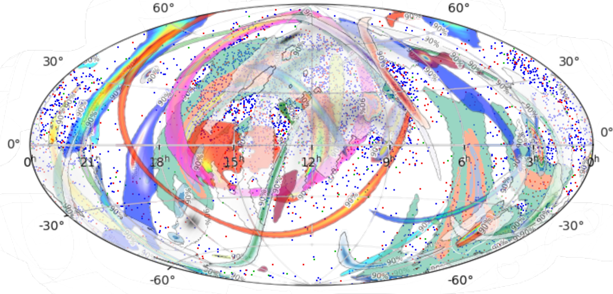
Figure 1: Positions of the AGN in CAT450 (blue dots), CAT455 (red dots), and CAT460 (green dots) described in Section 2.1, and 90 per cent CL localisation surfaces of the 30 detected BBH mergers listed in 2. These have a 90 per cent CI of the redshift posterior fully contained within $z=0.3$ (coloured regions). Regions with different colours correspond to different events. The sky map is visualized in equatorial coordinates.

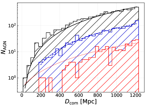
Figure 2: Number of AGN $N_{\rm AGN}$ in the catalogues presented in Section 2.1 as a function of comoving distance $D_{\rm com}$. The black, blue, and red histograms refer to CAT450, CAT455, and CAT460, respectively. The black solid line, the blue dashed one, and the red dotted one show the best fit functions we obtain when fitting the number of objects per bin using the following form: $N_{\rm AGN}\propto D_{\rm com}^{2}$. These fits show no evidence of a significant redshift-dependent incompleteness of the catalogues. The apparent dearth of objects with $D_{\rm com}\leq 400$ Mpc in CAT460 can be explained in terms of a random statistical fluctuation with respect to the expectation value.

A simple three-regions partition of the catalogues is used to identify areas with similar 2D sky-projected number density of AGN. For CAT455 we have that:

• 809 objects are within the footprint of the seventeenth data release of the Sloan Digital Sky Survey (SDSS) (York et al., 2000; Blanton et al., 2017; Abdurro’uf et al., 2022) (which corresponds approximately to 35.28 per cent of the sky). This is the most crowded region of the three, with a 2D number density of $\approx 0.0556$ objects per square degree;

• 41 objects are characterized by a galactic latitude $b$ with an absolute value smaller than $10^{\circ}$ (approximately 17.36 per cent of the sky). In this region the Galactic plane of the Milky Way prevents observations from detecting most of the extra-galactic content, and is therefore the least crowded region of our catalogue, with 2D number density of $\approx 0.0057$ objects per square degree;

• The remaining 562 objects populate the remaining 47.36 per cent of the sky. The average 2D number density in this region is $\approx 0.0288$ objects per square degree.

Because the AGN we consider and their host galaxies are relatively bright, many of them fall within the flux limit of the SDSS spectrocopic galaxy sample (Strauss et al., 2002), which has a completeness close to 100 per cent. In addition, the SDSS spectroscopic target selection (Richards et al., 2002) is tuned to target AGN or quasars below this flux limit. For this reason, the completeness of our catalogues in the SDSS footprint can be assumed to be close to 100 per cent. We calculate the incompleteness of the other two regions from the ratio of the projected 2D densities. Small deviations from unity for the completeness in the SDSS footprint are not expected to significantly change our final results. The same partition of the sky has been used to estimate the completeness of CAT450 and CAT460. The estimated completenesses, weighted over the area occupied by each region, are $\approx 48$ per cent, $\approx 61$ per cent, and $\approx 87$ per cent for CAT450, CAT455, and CAT460, respectively.

We calculate the number densities of the AGN catalogues we create, correcting for their completeness. We obtain a completeness-corrected number density of $1.53\cdot 10^{-6}{\rm Mpc}^{-3}$, $2.93\cdot 10^{-7}{\rm Mpc}^{-3}$, and $3.54\cdot 10^{-8}{\rm Mpc}^{-3}$ for CAT450, CAT455, and CAT460, respectively. To illustrate the content of our catalogues, we show in Table 1 as an example the first ten entries of CAT450.

Name Citation for Name unWISE ID R.A. Dec. $z$ Citation for $z$ W1 mag $L_{\rm W1}$ [deg] [deg] [${\rm erg\,s}^{-1}$] UVQSJ000000.15-200427.7 Monroe et al. (2016) 0000m197o0005716 $0.00065$ $-20.07433$ 0.291 Monroe et al. (2016) $13.65$ $2.72\cdot 10^{44}$ SDSS J000005.49+310527.6 Ahumada et al. (2020) 0000p318o0001234 $0.02290$ $31.09102$ 0.286 Ahumada et al. (2020) $14.20$ $1.58\cdot 10^{44}$ PHL 2525 Lamontagne et al. (2000) 0000m122o0001902 $0.10172$ $-12.76328$ $0.200$ Lamontagne et al. (2000) $11.04$ $1.29\cdot 10^{45}$ 2MASX J00004028-0541012 Masci et al. (2010) 0000m061o0015237 $0.16774$ $-5.68361$ $0.094$ Masci et al. (2010) $11.33$ $1.90\cdot 10^{44}$ RXS J00009+1723 Wei et al. (1999) 0000p166o0024250 $0.23319$ $17.39413$ $0.215$ Wei et al. (1999) $12.93$ $2.64\cdot 10^{44}$ SDSS J000102.18-102326.9 Lyke et al. (2020) 0000m107o0014745 $0.25911$ $-10.39078$ $0.294$ Lyke et al. (2020) $14.75$ $1.01\cdot 10^{44}$ RX J00013+0728 Tesch & Engels (2000) 0000p075o0010333 $0.32534$ $7.47432$ $0.270$ Tesch & Engels (2000) $14.06$ $1.57\cdot 10^{44}$ PGC 929358 Paturel et al. (2003) 0000m137o0004668 $0.33219$ $-14.07310$ $0.087$ Mauch & Sadler (2007) $11.65$ $1.21\cdot 10^{44}$ PGC 1698547 Paturel et al. (2003) 0000p242o0009501 $0.38474$ $24.04179$ $0.104$ Ahumada et al. (2020) $11.72$ $1.65\cdot 10^{44}$ RX J00015+0529 Tesch & Engels (2000) 0000p060o0003070 $0.38896$ $5.48926$ $0.250$ Ahumada et al. (2020) $12.67$ $4.71\cdot 10^{44}$

Table 1: First ten objects from our publicly available catalogue of AGN with a bolometric luminosity higher than $10^{45}\,{\rm erg\,s}^{-1}$, in ascending order of Right Ascension. For every object we indicate the original ID from the literature, the paper that first presented it, its unWISE ID, Right Ascension, Declination, redshift, the paper that first presented that redshift estimate, the magnitude in the W1 band, and the luminosity in the same band, $L_{\rm W1}$. We calculate the bolometric luminosity multiplying $L_{\rm W1}$ by a bolometric correction factor, approximated to 10 for this band and in the luminosity range we consider (Hopkins et al., 2007). Out of the 5,791 objects in the catalogue, a total of 3,561 have a redshift measurement obtained from SDSS. In particular, 1,582 of these measurements are taken from Lyke et al. (2020), 1,025 from Ahumada et al. (2020), and 954 from Liu et al. (2019). The full catalogue will be made available on the journal website and at https://github.com/niccoloveronesi/AGNallskycat_Veronesi23.git.

2.2 Detected Gravitational Wave events

When applying our statistical method to real data, we exploit the localisation volumes of 30 BBH mergers. These were detected during the first three observing runs of the LIGO and Virgo intereferometers. We select those with the 90 per cent CI of the redshift posterior distribution within $z=0.3$ and false alarm rate below 1 per year. Our selected events are among the ones used in The LIGO Scientific Collaboration et al. (2021b) to infer the parameters of the sMBH astrophysical population. These sky maps have been downloaded from the Gravitational Wave Open Science Center (Abbott et al., 2021b).

Event ID	$m_{1}$	$m_{2}$	$\chi_{\rm eff}$	$z$	SNR	${\rm V90}$	$N_{{\rm V90,CAT450}}$	$N_{{\rm V90,CAT455}}$	$N_{{\rm V90,CAT460}}$
	${\rm M}_{\odot}$	${\rm M}_{\odot}$				$\left[{\rm Mpc}^{3}\right]$
GW150914_095045	$34.6_{-2.6}^{+4.4}$	$30.0_{-4.6}^{+2.9}$	$-0.04_{-0.14}^{+0.12}$	$0.10_{-0.03}^{+0.03}$	$26.0_{-0.2}^{+0.1}$	$3.39\cdot 10^{6}$	3	0	0
GW151226_033853	$14.2_{-3.6}^{+11.1}$	$7.5_{-2.8}^{+2.4}$	$0.20_{-0.08}^{+0.23}$	$0.10_{-0.04}^{+0.03}$	$12.7_{-0.4}^{+0.3}$	$1.32\cdot 10^{7}$	10	1	0
GW170104_101158	$28.7_{-4.2}^{+6.6}$	$20.8_{-4.7}^{+4.1}$	$-0.04_{-0.19}^{+0.15}$	$0.22_{-0.09}^{+0.07}$	$13.8_{-0.3}^{+0.2}$	$1.42\cdot 10^{8}$	196	30	6
GW170608_020116	$10.6_{-1.4}^{+4.0}$	$7.8_{-1.9}^{+1.2}$	$0.05_{-0.05}^{+0.13}$	$0.07_{-0.03}^{+0.03}$	$15.3_{-0.3}^{+0.2}$	$2.98\cdot 10^{6}$	3	0	0
GW170809_082821	$34.1_{-5.3}^{+8.0}$	$24.2_{-5.3}^{+4.8}$	$0.07_{-0.17}^{+0.17}$	$0.21_{-0.07}^{+0.05}$	$12.8_{-0.3}^{+0.2}$	$4.21\cdot 10^{7}$	35	6	1
GW170814_103043	$30.9_{-3.3}^{+5.4}$	$24.9_{-4.0}^{+3.0}$	$0.08_{-0.12}^{+0.13}$	$0.13_{-0.05}^{+0.03}$	$17.7_{-0.3}^{+0.2}$	$2.96\cdot 10^{6}$	2	0	0
GW170818_022509	$34.8_{-4.2}^{+6.5}$	$27.6_{-5.1}^{+4.1}$	$-0.06_{-0.22}^{+0.19}$	$0.21_{-0.07}^{+0.07}$	$12.0_{-0.4}^{+0.3}$	$6.04\cdot 10^{6}$	3	1	0
GW190412_053044	$27.7_{-6.0}^{+6.0}$	$9.0_{-1.4}^{+2.0}$	$0.21_{-0.13}^{+0.12}$	$0.15_{-0.04}^{+0.04}$	$19.8_{-0.3}^{+0.2}$	$9.16\cdot 10^{6}$	20	3	0
GW190425_081805	$2.1_{-0.4}^{+0.5}$	$1.3_{-0.2}^{+0.3}$	$0.07_{-0.05}^{+0.07}$	$0.03_{-0.01}^{+0.02}$	$12.4_{-0.4}^{+0.4}$	$7.78\cdot 10^{6}$	9	1	0
GW190630_185205	$35.1_{-5.5}^{+6.5}$	$24.0_{-5.2}^{+5.5}$	$0.10_{-0.13}^{+0.14}$	$0.18_{-0.07}^{+0.09}$	$16.4_{-0.3}^{+0.2}$	$1.23\cdot 10^{8}$	148	33	4
GW190707_093326	$12.1_{-2.0}^{+2.6}$	$7.9_{-1.3}^{+1.6}$	$-0.04_{-0.09}^{+0.10}$	$0.17_{-0.08}^{+0.06}$	$13.1_{-0.4}^{+0.2}$	$9.20\cdot 10^{7}$	17	3	1
GW190708_232457	$19.8_{-4.3}^{+4.3}$	$11.6_{-2.0}^{+3.1}$	$0.05_{-0.10}^{+0.10}$	$0.19_{-0.07}^{+0.06}$	$13.4_{-0.3}^{+0.2}$	$1.02\cdot 10^{9}$	1560	305	43
GW190720_000836	$14.2_{-3.3}^{+5.6}$	$7.5_{-1.8}^{+2.2}$	$0.19_{-0.11}^{+0.14}$	$0.16_{-0.05}^{+0.11}$	$10.9_{-0.8}^{+0.3}$	$4.24\cdot 10^{7}$	20	7	1
GW190725_174728	$11.8_{-3.0}^{+10.1}$	$6.3_{-2.5}^{+2.1}$	$-0.04_{-0.16}^{+0.36}$	$0.20_{-0.08}^{+0.09}$	$9.1_{-0.7}^{+0.4}$	$3.81\cdot 10^{8}$	106	44	11
GW190728_064510	$12.5_{-2.3}^{+6.9}$	$8.0_{-2.6}^{+1.7}$	$0.13_{-0.07}^{+0.19}$	$0.18_{-0.07}^{+0.05}$	$13.1_{-0.4}^{+0.3}$	$3.88\cdot 10^{7}$	17	4	0
GW190814_211039	$23.3_{-1.4}^{+1.4}$	$2.6_{-0.1}^{+0.1}$	$0.00_{-0.07}^{+0.07}$	$0.05_{-0.01}^{+0.01}$	$25.3_{-0.2}^{+0.1}$	$3.55\cdot 10^{4}$	0	0	0
GW190917_033853	$9.7_{-3.9}^{+3.4}$	$2.1_{-0.4}^{+1.1}$	$-0.08_{-0.43}^{+0.21}$	$0.15_{-0.06}^{+0.05}$	$8.3_{-0.8}^{+0.5}$	$1.05\cdot 10^{8}$	60	22	3
GW190924_021846	$8.8_{-1.8}^{+4.3}$	$5.1_{-1.5}^{+1.2}$	$0.03_{-0.08}^{+0.20}$	$0.11_{-0.04}^{+0.04}$	$12.0_{-0.4}^{+0.3}$	$1.27\cdot 10^{7}$	13	1	0
GW190925_232845	$20.8_{-2.9}^{+6.5}$	$15.5_{-3.6}^{+2.5}$	$0.09_{-0.15}^{+0.16}$	$0.19_{-0.07}^{+0.08}$	$9.7_{-0.6}^{+0.3}$	$2.86\cdot 10^{8}$	401	94	12
GW190930_133541	$14.2_{-4.0}^{+8.0}$	$6.9_{-2.1}^{+2.4}$	$0.19_{-0.16}^{+0.22}$	$0.16_{-0.06}^{+0.06}$	$9.7_{-0.5}^{+0.3}$	$1.32\cdot 10^{8}$	63	13	2
GW191103_022549	$11.8_{-2.2}^{+6.2}$	$7.9_{-2.4}^{+1.7}$	$0.21_{-0.10}^{+0.16}$	$0.20_{-0.09}^{+0.09}$	$8.9_{-0.5}^{+0.3}$	$3.16\cdot 10^{8}$	255	62	8
GW191105_143512	$10.7_{-1.6}^{+3.7}$	$7.7_{-1.9}^{+1.4}$	$-0.02_{-0.09}^{+0.13}$	$0.23_{-0.09}^{+0.07}$	$9.7_{-0.5}^{+0.3}$	$1.53\cdot 10^{8}$	164	36	3
GW191129_134029	$10.7_{-2.1}^{+4.1}$	$6.7_{-1.7}^{+1.5}$	$0.06_{-0.08}^{+0.16}$	$0.16_{-0.06}^{+0.05}$	$13.1_{-0.3}^{+0.2}$	$5.92\cdot 10^{7}$	101	20	2
GW191204_171526	$11.9_{-1.8}^{+3.3}$	$8.2_{-1.6}^{+1.4}$	$0.16_{-0.05}^{+0.08}$	$0.13_{-0.05}^{+0.04}$	$17.5_{-0.2}^{+0.2}$	$1.24\cdot 10^{7}$	12	1	0
GW191216_213338	$12.1_{-2.3}^{+4.6}$	$7.7_{-1.9}^{+1.6}$	$0.11_{-0.06}^{+0.13}$	$0.07_{-0.03}^{+0.02}$	$18.6_{-0.2}^{+0.2}$	$3.66\cdot 10^{6}$	2	2	0
GW200115_042309	$5.9_{-2.5}^{+2.0}$	$1.44_{-0.29}^{+0.85}$	$-0.15_{-0.42}^{+0.24}$	$0.06_{-0.02}^{+0.09}$	$11.3_{-0.5}^{+0.3}$	$3.79\cdot 10^{6}$	3	2	0
GW200129_065458	$34.5_{-3.2}^{+9.9}$	$28.9_{-9.3}^{+3.4}$	$0.11_{-0.16}^{+0.11}$	$0.18_{-0.07}^{+0.05}$	$26.8_{-0.2}^{+0.2}$	$7.06\cdot 10^{6}$	7	0	0
GW200202_153413	$10.1_{-1.4}^{+3.5}$	$7.3_{-1.7}^{+1.1}$	$0.04_{-0.66}^{+0.13}$	$0.09_{-0.03}^{+0.03}$	$10.8_{-0.4}^{+0.2}$	$2.32\cdot 10^{6}$	2	0	0
GW200311_115853	$34.2_{-3.8}^{+6.4}$	$27.7_{-5.9}^{+4.1}$	$-0.02_{-0.20}^{+0.16}$	$0.23_{-0.07}^{+0.05}$	$17.8_{-0.2}^{+0.2}$	$5.94\cdot 10^{6}$	7	2	0
GW200316_215756	$13.1_{-2.9}^{+10.2}$	$7.8_{-2.9}^{+1.9}$	$0.13_{-0.10}^{+0.27}$	$0.22_{-0.08}^{+0.08}$	$10.3_{-0.7}^{+0.4}$	$9.22\cdot 10^{7}$	12	5	0

Table 2: List of the 30 BBH mergers detected during the first three observing runs of the LIGO and Virgo intereferometers with a CI of the redshift posterior contained within $z=0.3$ and a false alarm rate below 1 per year.

For every event, we report its ID, the mass of both the primary ($m_{1}$) and the secondary ($m_{2}$) component, the effective inspiral spin parameter $\chi_{\rm eff}$ (Ajith et al., 2011), the redshift, the SNR, and the value of V90. The last three columns correspond to the number of AGN inside V90, belonging to our three catalogues. We report the median and the 90 per cent credible intervals for the masses, the effective spin parameter, the redshift, and the SNR.

Table 2 lists these events. Among the parameters we report for each event, three are intrinsic properties of the binary. These are the masses of the two components of the binary, and the effective inspiral spin parameter. The latter is a weighted average of the projections of the two components’ spins on the direction of the angular momentum of the binary (for a more detailed description of this parameter, see Ajith et al., 2011; The LIGO Scientific Collaboration et al., 2021a, b). The other parameters reported for each detected GW event in Table 2 are the redshift, the SNR, V90, and the number of AGN from our all-sky observed catalogues that are inside V90. The 90 per cent CL sky regions of the same BBH mergers that are listed in Table 2 are displayed in Figure 1.

2.3 AGN mock catalogue

We test our statistical method explained below on an AGN mock catalogue characterized by a non-uniform incompleteness. In order to create it, we first have to construct a complete parent mock catalogue, where we assume that all AGN are accounted for. These are uniformly distributed in comoving volume between $z=0.0$ and $z=0.4$ with a number density of $n_{\rm AGN}=10^{-7}{\rm Mpc}^{-3}$. The non-uniform incomplete catalogue is a sub-sample of this complete one. Non-uniform incompleteness is a feature present also in the observed AGN catalogues exploited in this paper (see section 2.1). The incomplete mock catalogue is created by dividing the complete one in three different regions, and sub-sampling each of them in a different way as follows:

• The first region has galactic coordinate $b$ bigger than $30^{\circ}$. This corresponds to 25 per cent of the sky. In this first region no sub-sampling has been performed, hence its completeness is 100 per cent;

• The second region has $b$ between $-30^{\circ}$ and $30^{\circ}$. This corresponds to 50 per cent of the sky. In this second region, we remove 30 per cent of the objects from the parent complete catalogue, hence the completeness in this region is 70 per cent.

• The third region has Galactic coordinate $b$ smaller than $-30^{\circ}$. This corresponds to the remaining 25 per cent of the sky. Here we removed the 70 per cent of the objects from the complete catalogue, so the completeness of this region is 30 per cent.

The incomplete mock catalogue has a total of 1,160 objects, and a weighted average completeness of 67.5 per cent.

2.4 Simulated Gravitational Wave sky maps

The sky maps of our simulated GW events are described for simplicity as 3D Gaussian probability distributions. These distributions are created such that the size of their 90 per cent Credibility Level volume is the same as the size of an actual V90 simulated with the same source parameters, assuming the O3 configuration of the LIGO and Virgo detectors. For these simulated events we assume a Black Hole mass distribution that follows the Power Law + Peak model described in The LIGO Scientific Collaboration et al. (2021b). For simplicity the spins of the components of the binaries are assumed to be aligned with the binary angular momentum, with a magnitude uniformly distributed between $0$ and $1$. This choice does not bias our analysis. This is because assuming aligned spins leads to distributions of V90 consistent with the observed one (Veronesi et al., 2022). The size of V90 is the only parameter of the simulated BBH merger detections that enters the analysis presented in this paper, together with the spatial position. The inclination $\iota$ of the binaries is sampled from a uniform distribution in $\arccos{\iota}$. Once we have sampled the distributions of all the parameters of the merging BBH (masses and spins of the components, position of the merger and inclination of the binary), we model its GW signal with an IMRPhenomD waveform type (Husa et al., 2016; Khan et al., 2016). We then simulate the detection of this signal with a network composed of three interferometers: LIGO Hanford, LIGO Livingston, and Virgo. The sensitivity curves we use for these three detectors are the ones correspondent to the following IDs: aLIGOMidLowSensitivityP1200087 for the LIGO interferometers, and AdVMidLowSensitivityP1200087 for Virgo. The duty cycle indicates for what fraction of the total observing time each of the detectors is online. To all detectors, we assign the average value of the duty cycles that characterized the third observing run of LIGO and Virgo: 0.78 (Abbott et al., 2021a; The LIGO Scientific Collaboration et al., 2021a). We keep a Signal to Noise Ratio (SNR) detection threshold of 8 for the network, and require SNR$\geq 4$ for at least two of the three detectors. This cut leads to a realistic distribution of V90 (Veronesi et al., 2022), allowing us to circumvent the need to calculate the detection confidence level, according to the LIGO-Virgo-KAGRA collaboration criteria. We finally measure V90 for every simulated detection using the Bayestar algorithm (Singer & Price, 2016). The sensitivity curves used to create these simulated detections and the value chosen for the duty cycles aim to reproduce the network that performed real detections during the third observing run of the LIGO and Virgo interferometers (O3). However, we apply the method these simulations are used to test also to GW events detected before O3. This does not introduce any bias in the testing strategy described in Section 3.2, because there is no V90 from the first and second observing runs which is smaller (bigger) than the smallest (biggest) one from O3 (see Table 2).

To each simulated detection we therefore associate a value of V90. We call R90 the radius of a sphere of volume V90. The 3D spherically symmetric Gaussian distributions we use as mock GW sky maps are combinations of three 1D Gaussian distributions with equal standard deviation. For every value of R90, we calculate the standard deviation each of the 1D distributions must have in order for the 90 per cent credibility contour of the 3D Gaussian distribution to be a spherical surface of radius R90.

Knowing the exact position of each GW event we simulate, we can then sample the coordinates of the centre of the correspondent mock sky map from a Gaussian distribution centered on it. The standard deviation of such Gaussian is calculated from the value of R90 associated to the simulated BBH merger.

The sample of mock sky maps for the testing of our statistical method is therefore represented by 3D Gaussian distributions characterized by the positions of their centres and the radii of their 90 per cent credibility level regions (R90). The test strategy described in detail later in Section 3.2 is independent on the shape of the sky maps used during the cross match with mock AGN catalogues. For this reason, the choice of using a 3D Gaussian distribution does not lead to any bias in the obtained results concerning the test of the validity of the statistical method.

3 Method

3.1 Likelihood function

Our statistical framework compares two scenarios. In the first scenario AGN are physically associated to BBH mergers, while in the second one, AGN are background sources, i.e, their presence inside the the localisation volume of a GW event is coincidental.

The general analytical form of the likelihood function used in this work is based on the one described in Braun et al. (2008) and first used to draw conclusions on the detectability of a GW-AGN connection by Bartos et al. (2017). This can be written as follows:

$$\mathcal{L}\left(f_{\rm AGN}\right) =\prod_{i=1}^{N_{\rm GW}}\mathcal{L}_{i}\left(f_{\rm AGN}\right)$$

$$=\prod_{i=1}^{N_{\rm GW}}\left[c\cdot 0.9\cdot f_{\rm AGN}\cdot\mathcal{S}_{i}+\left(1-c\cdot 0.90\cdot f_{\rm AGN}\right)\mathcal{B}_{i}\right]\ \ ,$$ (1)

where $\mathcal{L}_{i}$ is the single-event likelihood associated to the $i$-th GW event, $f_{\rm AGN}$ is the fraction of GW events that originate from an AGN, $N_{\rm GW}$ is the total number of GW events, $c$ is the average completeness of the AGN catalogue, and $\mathcal{S}_{i}$ ($\mathcal{B}_{i}$) is the signal (background) probability density function. If the value of $\mathcal{S}_{i}$ is bigger than the value of $\mathcal{B}_{i}$, $\mathcal{L}_{i}\left(f_{\rm AGN}\right)$ will peak at the maximum allowed value of its parameter: $f_{\rm AGN}=1$, meaning that the $i$-th GW event is likely physically associated to one of the AGN that are inside its localisation volume. The opposite is true if if the value of $\mathcal{B}_{i}$ is bigger than the value of $\mathcal{S}_{i}$. The product of all the single-event likelihoods is then what determines the degree of GW-AGN association through the value of $f_{\rm AGN}$ corresponding to its maximum. The $0.9$ pre-factor in front of $f_{\rm AGN}$ is used to take into account that the localisation volumes we use are associated to a confidence level of 90 per cent. The introduction of the $c$ factor is a novelty with respect to previous similar works that used only complete mock AGN catalogues (Bartos et al., 2017; Corley et al., 2019; Veronesi et al., 2022). If such a term was not present when using incomplete catalogues, the likelihood function would on average peak at a lower value of $f_{\rm AGN}$ with respect to the true one. This would happen because, even if a physical association exists, it might not be detected if the AGN host of a GW event is not present in the catalogue. The $c$ factor in Equation 1 corrects for this potential bias. Previous studies used as main input the size of each GW event’s V90 and the number of AGN within it ($N_{{\rm V90}}$). In this work, we additionally exploit the information embedded in the exact position of every AGN within the localisation volume: i.e., the value of the 3D GW localisation probability density function at the AGN position. We therefore write the signal probability density function for the $i$-th GW as:

$$\mathcal{S}_{i}=\frac{\sum_{j=1}^{N_{{\rm V90}_{i}}}p_{j}}{n_{\rm AGN}{\rm V90}_{i}}\ \ ,$$ (2)

where $n_{\rm AGN}$ is the average number density of AGN in the catalogue, and $p_{j}$ is the probability density associated to the position of the $j$-th AGN. The denominator in Equation 2 represents the expected number of AGN from a catalogue of number density $n_{\rm AGN}$ that are contained in a region of size ${\rm V90}_{i}$. Therefore, the signal probability density function represents the total probability density associated to the positions of all the AGN within ${\rm V90}_{i}$, normalized by their expected number. The more objects there are within ${\rm V90}_{i}$ and/or the more clustered they are towards the peak of the probability density distribution, the higher the value of $\mathcal{S}_{i}$ is. This is in accord with the fact that $\mathcal{S}_{i}$ in Equation 2 describes how likely the scenario in which AGN are physically associated to BBH mergers is. On the other hand, the probability density function associated to the scenario where AGN are background sources, accidentally present in GW localisation volumes, can be expressed with a flat probability for an AGN to be found anywhere in V90:

$$\mathcal{B}_{i}=\frac{0.9}{{\rm V90}_{i}}\ \ ,$$ (3)

where the $0.9$ term at the numerator guarantees that $\mathcal{S}_{i}$ and $\mathcal{B}_{i}$ are normalized to the same value. From Equations 2 and 3 it follows that the likelihood function in Equation 1 is dimensionful with units of one over volume. This means that for it to be turned into a probability density function, it should be normalized dividing it by its integral over the whole [0,1] range of $f_{\rm AGN}$. During the testing of the statistical method on mock data and its application to real GW detections and AGN catalogues the non-normalized version of the likelihood function is usually computed, unless specified otherwise. In particular we normalize this function when extracting the posterior distribution on $f_{\rm AGN}$.

In our statistical analysis the prior on $f_{\rm AGN}$ is assumed to be uniform between 0 and 1.

3.2 Test on mock data

To test the performance of the likelihood we use data coming from the cross-match between the incomplete AGN mock catalogue described in Section 2.3 and the mock GW detections described in Section 2.4.

This test consists of a Monte Carlo simulation of 1,000 realizations. Every realization is characterized by the same total number of simulated detected BBH mergers. This number of detections is the same one used during the application to real data: $N_{\rm GW}=30$. At the start of each realization, we draw a value from the prior distribution of $f_{\rm AGN}$. This represents the true value of this parameter for the specific realization, and will be further referred to as $f_{\rm AGN,true}$. We then sample a binomial distribution characterized by the parameters $n=N_{\rm GW}$ and $p=f_{\rm AGN,true}$ to obtain the number of simulated detected GWs that come from an AGN of the complete mock catalogue presented in Section 2.3 within $z=0.2$. The remaining events of the $N_{\rm GW}$ simulated detections are the ones coming from a position randomly sampled from a uniform distribution in the same redshift range. The redshift cut on the potential sources of both the signal and the background events is performed to be sure that the entirety of V90 is within the volume of the mock AGN catalogue. This is necessary to avoid any boundary-related underestimation of $\mathcal{S}_{i}$ during the cross-match of these localisation volumes with the incomplete AGN mock catalogue.

We cross-match the 3D Gaussian distributions representing the sky maps of the 30 GW events with the incomplete AGN mock catalogue and calculate the value of the likelihood as a function of $f_{\rm AGN}$ using Equations 1, 2, and 3. We then compute the normalized posterior distribution on $f_{\rm AGN}$: $\mathcal{P}\left(f_{\rm AGN}\right)$. Finally, we calculate the Credibility Level (CL) of $f_{\rm AGN,true}$ and the corresponding Credibility Interval (CI). The CI is defined as the range of $f_{\rm AGN}$ that is associated to values of the posterior equal or greater than $\mathcal{P}\left(f_{\rm AGN,true}\right)$. We say for example that $f_{\rm AGN,true}$ has a CL of 90 per cent if the integral of $\mathcal{P}\left(f_{\rm AGN}\right)$ evaluated over the corresponding CI is $0.9$.

The blue line in the Probabilty-Probability plot presented in Figure 3 shows the cumulative distribution of the 1,000 values of CLs associated to $f_{\rm AGN,true}$ from all the realizations. The grey lines show the cumulative distribution of 100 uniform samples between 0 and 1. Since the distribution of the CLs associated to $f_{\rm AGN,true}$ is statistically indistinguishable from a uniform one, we can conclude that our statistical method is able to produce trustworthy results when tested on mock data. Therefore, maximizing the likelihood described in Equations 1, 2 and 3 leads to an accurate estimate of $f_{\rm AGN}$.

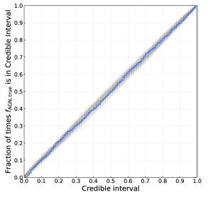
Figure 3: Fraction of times $f_{\rm AGN,true}$ lies within a certain Credible Interval as a function of the credibility level of such an interval. The blue line shows the result obtained by testing the likelihood function described in Section 3.1 on mock data. The gray lines show the cumulative distributions of 100 samples of a uniform distribution in the [0,1] range.

Finally, we test that our results do not change if we use in Equation 1 the actual value of the catalogue completeness ($c$) in each localisation volume. More specifically, this individual completeness is calculated as a weighted average of the completeness of the AGN catalogue in the 3D region occupied by each V90. Our test yields indistinguishable results, therefore, for simplicity, we only present the ones computed using the average catalogue completeness.

3.3 Application to real data

Once we have tested the accuracy of the statistical method, we apply it to real data. We cross-match the skymaps of the 30 detected BBH mergers presented in 2.2, and listed in Table 2 with the all-sky AGN catalogues described in Section 2.1. We then calculate $\mathcal{L}\left(f_{\rm AGN}\right)$ using Equations 1, 2, and 3.

In the case of CAT455 and CAT460 the combination of the data coming from the cross-match with the 30 GW events leads to a monotonically decreasing likelihood, as a function of $f_{\rm AGN}$. We therefore decide to evaluate upper limits on this parameter integrating the normalized likelihood between $f_{\rm AGN}=0$ and $f_{\rm AGN}=1$. Since the prior is assumed to be uniform, through this integration we obtain the cumulative posterior distribution on $f_{\rm AGN}$.

The same process has been followed also for CAT450, even if in this case the likelihood turns out to be rather insensitive to $f_{\rm AGN}$. Specifically, in this last case, the posterior is prior-dominated: data do not allow us to put much tighter constraints on $f_{\rm AGN}$ than the ones imposed by the flat prior only. This is caused by the high number of objects contained in the AGN catalogue (Veronesi et al., 2022), combined with the non-negligible level of incompleteness that characterizes the same catalogue. We therefore decide not to repeat the analysis with an AGN catalogue characterized by a lower luminosity threshold. Such a catalogue would likely also show redshift-dependent completeness, which will have to be taken into account in future works aimed to explore the relation between BBH mergers and lower-luminosities AGN. A meaningful exploitation of AGN catalogues denser than the ones used in this work will be possible only when we will have data from more and/or better localized BBH mergers.

4 Results

The cumulative posterior distributions over $f_{\rm AGN}$ we obtain through the application of our statistical method to observed data are shown in Figure 4.

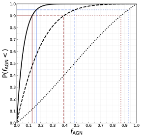
Figure 4: Black solid line: Cumulative posterior distribution for the fraction of detected GWs originated in an AGN ($f_{\rm AGN}$) with a bolometric luminosity higher than $10^{46}\,{\rm erg\,s}^{-1}$. Every value on the vertical axis corresponds to the probability associated to the true value of $f_{\rm AGN}$ being smaller than the correspondent value on the horizontal axis. The dashed (dotted) line shows the posterior distribution obtained using a luminosity threshold of $10^{45.5}\,{\rm erg\,s}^{-1}$ ($10^{45}\,{\rm erg\,s}^{-1}$). The maroon lines indicate that the upper limit of the 90 per cent credibility interval corresponds to $f_{\rm AGN}=0.13$ for the $10^{46}\,{\rm erg\,s}^{-1}$ luminosity cut, to $f_{\rm AGN}=0.40$ for the $10^{45.5}\,{\rm erg\,s}^{-1}$ luminosity cut, and to $f_{\rm AGN}=0.87$ for the $10^{45}\,{\rm erg\,s}^{-1}$ luminosity cut. The blue lines indicate that the upper limit of the 95 per cent credibility interval corresponds to $f_{\rm AGN}=0.17$ for the $10^{46}\,{\rm erg\,s}^{-1}$ luminosity cut, to $f_{\rm AGN}=0.49$ for the $10^{45.5}\,{\rm erg\,s}^{-1}$ luminosity cut, and to $f_{\rm AGN}=0.94$ for the $10^{45}\,{\rm erg\,s}^{-1}$ luminosity cut.

The black solid line shows the posterior distribution in the case of the cross-math of the observed GW events with CAT460, while the dashed (dotted) line shows it in the case of a CAT455 (CAT450). On the vertical axis there is the probability for the true value of $f_{\rm AGN}$ being smaller than the correspondent value on the horizontal axis. As an example, the solid blue line shows that the upper limit of the 95 per cent credibility interval is $f_{\rm AGN}=0.17$ in the case of the cross-match with CAT460.

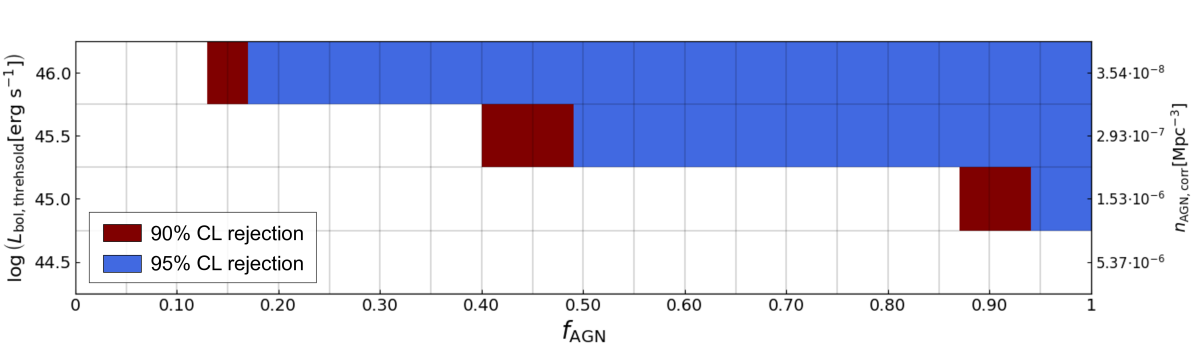
Figure 5: Rejected regions at 90 and 95 per cent credibility level of the two-dimensional parameter space $\{L_{\rm bol},f_{\rm AGN}\}$ investigated in this work. The bolometric luminosity threshold for the observed AGN is indicated on the vertical axis on the left-hand side, while the fraction of detected BBH mergers that come from AGN brighter than those thresholds is on the horizontal axis. The maroon (blue) regions are the ones that the analysis presented in this work rejects with a 90 (95) per cent credibility. The right vertical axis shows the number density obtained from the Hopkins et al. (2007) luminosity function, normalized to match the completeness-corrected number density of our catalogue.

Figure 5 shows a region of the two-dimensional parameter space that has been investigated in this work. On the vertical axis one can read the thresholds in bolometric luminosities of AGN on the left-hand side, and the correspondent values of number densities on the right-hand side. The three number densities correspondent to the three luminosity thresholds we use to create CAT450, CAT455, and CAT460 have been calculated taking into account their estimated completeness. For each of these completeness-corrected number densities we calculate their ratio with respect to the number density obtained integrating in the same luminosity range the best-fit AGN luminosity function at $z=0.1$ presented in Hopkins et al. (2007). The mean of this ratios, together with the number density estimated from Hopkins et al. (2007) for a bolometric luminosity threshold of $10^{44.5}\,{\rm erg\,s}^{-1}$, has been used to calculate the completeness-corrected number density for such a luminosity cut. All the possible values of $f_{\rm AGN}$ are on the horizontal axis. The maroon (blue) region is the part of the parameter space that we reject with a 90 (95) per cent credibility level.

In The LIGO Scientific Collaboration et al. (2021b) the total BBH merger rate per comoving volume has been parametrized as a power law as a function of redshift: $\mathcal{R}(z)\propto(1+z)^{\kappa}$. The value of the spectral index has been estimated to be $\kappa=2.7_{-1.9}^{+1.8}$, and the best measurement of the merger rate $\mathcal{R}$ occurs at $z\approx 0.2$: $\mathcal{R}(z=0.2)\leq 41\ {\rm Gpc}^{-3}{\rm yr}^{-1}$ at 90 per cent credibility. Combining this result with the upper limit of $f_{\rm AGN}\leq 0.49$ ($f_{\rm AGN}\leq 0.17$) obtained in this work, we find that the 95 per cent credibility upper limit on the rate of BBHs merging in AGN brighter than $10^{45.5}\,{\rm erg\,s}^{-1}$ ($10^{46}\,{\rm erg\,s}^{-1}$) is $\mathcal{R}_{\rm AGN}(z=0.2)\simeq 20\ {\rm Gpc}^{-3}{\rm yr}^{-1}$ ($\mathcal{R}_{\rm AGN}(z=0.2)\simeq 7\ {\rm Gpc}^{-3}{\rm yr}^{-1}$) at $z\approx 0.2$. It is important to remember that these results have been obtained assuming 100 per cent completeness in the SDSS footprint in our catalogues of luminous, redshift selected AGN. However, small variations over this assumption are not expected to produce qualitatively different results with respect to the ones presented in this section, since they scale linearly with the AGN catalogue completeness (see Equation 1).

5 Discussion and conclusion

We present a likelihood-based method to constrain the fractional contribution of the AGN channel to the observed merger rate of BBHs. In particular we compare the scenario in which AGN are physically associated to BBH mergers to the one in which the presence of AGN in localisation volumes of GW events is only due by chance. We use as input data the size of each GW localisation volume and the exact position of all the AGN that are in it. We calculate the posterior distribution of the fraction of the detected GW events that come from an AGN, $f_{\rm AGN}$. We then put observational constraints on this parameter by determining the upper limits associated to the 90 and 95 per cent CIs of the posterior distribution.

We first validate this method on a mock AGN catalogue characterized by a non-uniform completeness (see Figure 3).

We then apply the same statistical analysis to observed data. We use the sky maps of the 30 BBH mergers detected by the LIGO and Virgo interferometers characterized by a 90 per cent C.I. of the redshift distribution entirely contained within $z=0.3$. We cross-match these sky maps with three all-sky catalogues of AGN we create starting from cross-matching the unWISE catalogue (Schlafly et al., 2019) with the Milliquas one (Flesch, 2021). We select only the objects with a spectroscopic measurement of redshift correspondent to $z\leq 0.3$ and with a bolometric luminosity higher than $10^{45}\,{\rm erg\,s}^{-1}$, $10^{45.5}\,{\rm erg\,s}^{-1}$, and $10^{46}\,{\rm erg\,s}^{-1}$. We calculate the posterior cumulative distribution on $f_{\rm AGN}$ and conclude that in the case of the two highest luminosity thresholds we can put upper limits on this parameter that are tighter with respect to the ones one can obtain from the sole assumption of a uniform prior between 0 and 1. In the case of the cross-match with the AGN catalogue characterized by the highest (intermediate) luminosity threshold we find that $f_{\rm AGN}=0.17$ ($f_{\rm AGN}=0.49$) is the upper limit of the 95 per cent credibility interval. Figure 4 shows the entire cumulative posterior distributions, while Figure 5 shows more explicitly which parts of the two-dimensional AGN luminosity-$f_{\rm AGN}$ parameter space are rejected with a 90 and a 95 per cent credibility. Previous works used only simulated GW data and mock AGN catalogues to draw conclusions about the possibility of exploring the spatial correlation between the two. Instead, we present the first constraints on $f_{\rm AGN}$ based on observational data only. Moreover, in the previous analyses the number of potential hosts within the V90 of every GW event was used as the main source of information, together with the size of V90. As mentioned above, the likelihood function we present in this work also takes into account for the first time the exact position of every AGN within V90 and the overall completeness of the AGN catalogue. The results obtained in this work are observational upper limits on the correlation between the detected BBH mergers and the high luminosity, and spectroscopically selected AGN that are in the catalogues described in Section 2.1. They can be used in the future to inform theoretical models of compact binary objects in AGN discs. Such results hint towards the conclusion that physical conditions of the gas and the stars in the discs of high-luminosity AGN are not sufficiently able to drive the formation and the merger of binaries of sMBHs in order to be major contributors to the total merger rate. This conclusion would be in agreement with the recent theoretical result obtained by Grishin et al. (2023), where it is stated that migration traps in AGN discs are not expected to be present in the case of a bolometric luminosity higher than $10^{45}\ {\rm erg\ s}^{-}1$ for an AGN alpha viscosity parameter of $\alpha=0.01$. Their inability to create migration traps would explain why AGN characterized by a luminosity higher than such a threshold are not to be considered potential preferred hosts of BBH mergers.

One way for generalizing the results presented in this paper is the creation of a more complete all-sky AGN catalogue. The introduction of objects with only a photometric measurement of the redshift is a possible method of doing that. This would increase the number density of the catalogue, but will also increase the probability of considering objects that have been erraneously identified as AGN. This confidence on the classification of each object will have to be taken into account in the expression of the likelihood function.

The results concerning the posterior distributions shown in Figure 4 are relative to the fraction of BBH mergers that have happened in an AGN with a bolometric luminosity higher than the three thresholds we have considered. We perform this luminosity cuts in order to be sure to have a good level of completeness in our observed AGN catalogues. In order to draw general conclusion on the AGN formation channel for BBHs, future works will investigate the correlation between GW events and AGN in a broader range of luminosities. Such an investigation will have to take into consideration the fact that low values of complenetess and its dependence on redshift lower the statistical power of the method, increasing the uncertainty on the predictions.

The analysis described in this paper is restricted to BBH mergers whose host environment is expected to be at $z\leq 0.3$ with 90 per cent credibility. This selection has been done because a higher level of completeness for catalogues of observed AGN can be reached if we restrict our analysis to the local Universe. Future works might explore the GW-AGN correlation on a wider redshift range. The effectiveness of their results will be increased because of the possible exploitation of more detected BBH mergers, but might also be dampened by low levels of completeness of the considered AGN catalogues.

Dedicated tests performed by varying the different parameters in the Monte Carlo analysis described in Section 3.2 have proven that the prediction power of the method presented in this work depends mainly on three elements: the completeness of the AGN catalogue, the number of GW detections, and the size of their localisation volumes. Observational limitations (e.g. the presence of the Milky Way plane that does not allow the detection of light coming from objects behind it) prevent us from having an AGN catalogue with a completeness level close to unity. On the other hand, $79^{+89}_{-44}$ BBH mergers are expected to be observed via GWs during the fourth observing run (O4) of the LIGO-Virgo-KAGRA collaboration (Abbott et al., 2020), and at least the same amount of detections can be predicted for the fifth observing run (O5). This would at least triple the amount of detected events available for statistical analyses on the BBH population. This increase of the number of detections, together with the improvement on the localisation power expected for O4 and O5 with respect to previous observing runs, will noticeably increase the prediction power of likelihood-based methods like the one presented in this paper, that will be able to put more stringent constraints on the fractional contribution of high-luminosity AGN to the total BBH merger rate, and to make use of also denser catalogues of potential hosts, such as the ones containing AGN with luminosities lower than the ones considered in this work.

Data Availabilty

The data underlying this article are available in niccoloveronesi/AGNallskycat_Veronesi23, at https://github.com/niccoloveronesi/AGNallskycat_Veronesi23.git.

References

- Abbott et al. (2020) Abbott B. P., et al., 2020, Living Reviews in Relativity, 23, 3
- Abbott et al. (2021a) Abbott R., et al., 2021a, Physical Review X, 11, 021053
- Abbott et al. (2021b) Abbott R., et al., 2021b, SoftwareX, 13, 100658
- Abdurro’uf et al. (2022) Abdurro’uf et al., 2022, ApJS, 259, 35
- Acernese et al. (2015) Acernese F., et al., 2015, Classical and Quantum Gravity, 32, 024001
- Ahumada et al. (2020) Ahumada R., et al., 2020, ApJS, 249, 3
- Ajith et al. (2011) Ajith P., et al., 2011, Phys. Rev. Lett., 106, 241101
- Antonini et al. (2019) Antonini F., Gieles M., Gualandris A., 2019, MNRAS, 486, 5008
- Ashton et al. (2021) Ashton G., Ackley K., Hernandez I. M., Piotrzkowski B., 2021, Classical and Quantum Gravity, 38, 235004
- Assef et al. (2013) Assef R. J., et al., 2013, ApJ, 772, 26
- Astropy Collaboration et al. (2013) Astropy Collaboration et al., 2013, A&A, 558, A33
- Astropy Collaboration et al. (2018) Astropy Collaboration et al., 2018, AJ, 156, 123
- Barrera & Bartos (2022) Barrera O., Bartos I., 2022, ApJ, 929, L1
- Bartos (2016) Bartos I., 2016, in American Astronomical Society Meeting Abstracts #228. p. 208.03
- Bartos et al. (2017) Bartos I., Haiman Z., Marka Z., Metzger B. D., Stone N. C., Marka S., 2017, Nature Communications, 8, 831
- Belczynski et al. (2016) Belczynski K., et al., 2016, A&A, 594, A97
- Belczynski et al. (2022) Belczynski K., Doctor Z., Zevin M., Olejak A., Banerje S., Chattopadhyay D., 2022, ApJ, 935, 126
- Bellovary et al. (2016) Bellovary J. M., Mac Low M.-M., McKernan B., Ford K. E. S., 2016, ApJ, 819, L17
- Blanton et al. (2017) Blanton M. R., et al., 2017, AJ, 154, 28
- Braun et al. (2008) Braun J., Dumm J., De Palma F., Finley C., Karle A., Montaruli T., 2008, Astroparticle Physics, 29, 299
- Corley et al. (2019) Corley K. R., et al., 2019, MNRAS, 488, 4459
- Costa et al. (2021) Costa G., Bressan A., Mapelli M., Marigo P., Iorio G., Spera M., 2021, MNRAS, 501, 4514
- DeLaurentiis et al. (2022) DeLaurentiis S., Epstein-Martin M., Haiman Z., 2022, arXiv e-prints, p. arXiv:2212.02650
- Fabj et al. (2020) Fabj G., Nasim S. S., Caban F., Ford K. E. S., McKernan B., Bellovary J. M., 2020, MNRAS, 499, 2608
- Fishbach et al. (2022) Fishbach M., Kimball C., Kalogera V., 2022, ApJ, 935, L26
- Flesch (2021) Flesch E. W., 2021, VizieR Online Data Catalog, p. VII/290
- Ford & McKernan (2022) Ford K. E. S., McKernan B., 2022, MNRAS, 517, 5827
- Gayathri et al. (2021) Gayathri V., Yang Y., Tagawa H., Haiman Z., Bartos I., 2021, ApJ, 920, L42
- Gayathri et al. (2023) Gayathri V., Wysocki D., Yang Y., Shaughnessy R. O., Haiman Z., Tagawa H., Bartos I., 2023, arXiv e-prints, p. arXiv:2301.04187
- Gerosa & Berti (2017) Gerosa D., Berti E., 2017, Phys. Rev. D, 95, 124046
- Gerosa & Berti (2019) Gerosa D., Berti E., 2019, Phys. Rev. D, 100, 041301
- Gerosa & Fishbach (2021) Gerosa D., Fishbach M., 2021, Nature Astronomy, 5, 749
- Graham et al. (2020) Graham M. J., et al., 2020, Phys. Rev. Lett., 124, 251102
- Graham et al. (2023) Graham M. J., et al., 2023, ApJ, 942, 99
- Grishin et al. (2023) Grishin E., Gilbaum S., Stone N. C., 2023, arXiv e-prints, p. arXiv:2307.07546
- Harris et al. (2020) Harris C. R., et al., 2020, Nature, 585, 357
- Heger & Woosley (2002) Heger A., Woosley S. E., 2002, ApJ, 567, 532
- Hills & Fullerton (1980) Hills J. G., Fullerton L. W., 1980, AJ, 85, 1281
- Hopkins et al. (2007) Hopkins P. F., Richards G. T., Hernquist L., 2007, ApJ, 654, 731
- Hunter (2007) Hunter J. D., 2007, Computing in Science and Engineering, 9, 90
- Husa et al. (2016) Husa S., Khan S., Hannam M., Pürrer M., Ohme F., Forteza X. J., Bohé A., 2016, Phys. Rev. D, 93, 044006
- Karathanasis et al. (2022) Karathanasis C., Mukherjee S., Mastrogiovanni S., 2022, arXiv e-prints, p. arXiv:2204.13495
- Khan et al. (2016) Khan S., Husa S., Hannam M., Ohme F., Pürrer M., Forteza X. J., Bohé A., 2016, Phys. Rev. D, 93, 044007
- Kritos et al. (2022) Kritos K., Berti E., Silk J., 2022, arXiv e-prints, p. arXiv:2212.06845
- LIGO Scientific Collaboration et al. (2015) LIGO Scientific Collaboration et al., 2015, Classical and Quantum Gravity, 32, 074001
- Lamontagne et al. (2000) Lamontagne R., Demers S., Wesemael F., Fontaine G., Irwin M. J., 2000, AJ, 119, 241
- Li & Lai (2022a) Li R., Lai D., 2022a, arXiv e-prints, p. arXiv:2207.01125
- Li & Lai (2022b) Li R., Lai D., 2022b, MNRAS, 517, 1602
- Li et al. (2022) Li G.-P., Lin D.-B., Yuan Y., 2022, arXiv e-prints, p. arXiv:2211.11150
- Liu et al. (2019) Liu H.-Y., Liu W.-J., Dong X.-B., Zhou H., Wang T., Lu H., Yuan W., 2019, ApJS, 243, 21
- Loeb (2016) Loeb A., 2016, ApJ, 819, L21
- Lyke et al. (2020) Lyke B. W., et al., 2020, ApJS, 250, 8
- Mahapatra et al. (2022) Mahapatra P., Gupta A., Favata M., Arun K. G., Sathyaprakash B. S., 2022, arXiv e-prints, p. arXiv:2209.05766
- Mapelli (2021) Mapelli M., 2021, arXiv e-prints, p. arXiv:2106.00699
- Masci et al. (2010) Masci F. J., Cutri R. M., Francis P. J., Nelson B. O., Huchra J. P., Heath Jones D., Colless M., Saunders W., 2010, Publ. Astron. Soc. Australia, 27, 302
- Mauch & Sadler (2007) Mauch T., Sadler E. M., 2007, VizieR Online Data Catalog, p. J/MNRAS/375/931
- McKernan et al. (2011) McKernan B., Ford K. E. S., Lyra W., Perets H. B., Winter L. M., Yaqoob T., 2011, MNRAS, 417, L103
- McKernan et al. (2012) McKernan B., Ford K. E. S., Lyra W., Perets H. B., 2012, MNRAS, 425, 460
- McKernan et al. (2019) McKernan B., et al., 2019, ApJ, 884, L50
- McKernan et al. (2020) McKernan B., Ford K. E. S., O’Shaugnessy R., Wysocki D., 2020, MNRAS, 494, 1203
- McKernan et al. (2022) McKernan B., Ford K. E. S., Cantiello M., Graham M., Jermyn A. S., Leigh N. W. C., Ryu T., Stern D., 2022, MNRAS, 514, 4102
- Monroe et al. (2016) Monroe T. R., Prochaska J. X., Tejos N., Worseck G., Hennawi J. F., Schmidt T., Tumlinson J., Shen Y., 2016, AJ, 152, 25
- Palenzuela et al. (2010) Palenzuela C., Lehner L., Yoshida S., 2010, Phys. Rev. D, 81, 084007
- Paturel et al. (2003) Paturel G., Petit C., Prugniel P., Theureau G., Rousseau J., Brouty M., Dubois P., Cambrésy L., 2003, A&A, 412, 45
- Peng & Chen (2021) Peng P., Chen X., 2021, MNRAS, 505, 1324
- Petrov et al. (2022) Petrov P., et al., 2022, ApJ, 924, 54
- Planck Collaboration et al. (2016) Planck Collaboration et al., 2016, A&A, 594, A13
- Qin et al. (2022) Qin Y., et al., 2022, ApJ, 941, 179
- Richards et al. (2002) Richards G. T., et al., 2002, AJ, 123, 2945
- Rodriguez & Loeb (2018) Rodriguez C. L., Loeb A., 2018, ApJ, 866, L5
- Rodriguez et al. (2016) Rodriguez C. L., Chatterjee S., Rasio F. A., 2016, Phys. Rev. D, 93, 084029
- Rodriguez et al. (2021) Rodriguez C. L., Kremer K., Chatterjee S., Fragione G., Loeb A., Rasio F. A., Weatherford N. C., Ye C. S., 2021, Research Notes of the American Astronomical Society, 5, 19
- Romero-Shaw et al. (2021) Romero-Shaw I., Lasky P. D., Thrane E., 2021, ApJ, 921, L31
- Romero-Shaw et al. (2022) Romero-Shaw I., Lasky P. D., Thrane E., 2022, ApJ, 940, 171
- Rowan et al. (2022) Rowan C., Boekholt T., Kocsis B., Haiman Z., 2022, arXiv e-prints, p. arXiv:2212.06133
- Samsing et al. (2022) Samsing J., et al., 2022, Nature, 603, 237
- Schlafly et al. (2019) Schlafly E. F., Meisner A. M., Green G. M., 2019, ApJS, 240, 30
- Singer & Price (2016) Singer L. P., Price L. R., 2016, Phys. Rev. D, 93, 024013
- Stern et al. (2012) Stern D., et al., 2012, ApJ, 753, 30
- Stevenson & Clarke (2022) Stevenson S., Clarke T. A., 2022, MNRAS, 517, 4034
- Stone et al. (2017) Stone N. C., Metzger B. D., Haiman Z., 2017, MNRAS, 464, 946
- Strauss et al. (2002) Strauss M. A., et al., 2002, AJ, 124, 1810
- Tagawa et al. (2020) Tagawa H., Haiman Z., Kocsis B., 2020, ApJ, 898, 25
- Tagawa et al. (2021) Tagawa H., Haiman Z., Bartos I., Kocsis B., Omukai K., 2021, MNRAS, 507, 3362
- Tanikawa et al. (2021) Tanikawa A., Susa H., Yoshida T., Trani A. A., Kinugawa T., 2021, ApJ, 910, 30
- Tesch & Engels (2000) Tesch F., Engels D., 2000, MNRAS, 313, 377
- The LIGO Scientific Collaboration et al. (2021a) The LIGO Scientific Collaboration et al., 2021a, arXiv e-prints, p. arXiv:2111.03606
- The LIGO Scientific Collaboration et al. (2021b) The LIGO Scientific Collaboration et al., 2021b, arXiv e-prints, p. arXiv:2111.03634
- Vajpeyi et al. (2022) Vajpeyi A., Thrane E., Smith R., McKernan B., Saavik Ford K. E., 2022, ApJ, 931, 82
- Veronesi et al. (2022) Veronesi N., Rossi E. M., van Velzen S., Buscicchio R., 2022, MNRAS, 514, 2092
- Virtanen et al. (2020) Virtanen P., et al., 2020, Nature Methods, 17, 261
- Wang et al. (2021) Wang Y.-Z., Fan Y.-Z., Tang S.-P., Qin Y., Wei D.-M., 2021, arXiv e-prints, p. arXiv:2110.10838
- Wang et al. (2022) Wang Y., McKernan B., Ford K. E. S., Perna R., Leigh N., Mac Low M.-M., 2022, in AAS/Division of Dynamical Astronomy Meeting. p. 300.01
- Wei et al. (1999) Wei J. Y., Xu D. W., Dong X. Y., Hu J. Y., 1999, A&AS, 139, 575
- Woosley (2019) Woosley S. E., 2019, ApJ, 878, 49
- Wright et al. (2010) Wright E. L., et al., 2010, AJ, 140, 1868
- Yang et al. (2019) Yang Y., et al., 2019, Phys. Rev. Lett., 123, 181101
- York et al. (2000) York D. G., et al., 2000, AJ, 120, 1579
- Zevin & Bavera (2022) Zevin M., Bavera S. S., 2022, ApJ, 933, 86
- Ziosi et al. (2014) Ziosi B. M., Mapelli M., Branchesi M., Tormen G., 2014, MNRAS, 441, 3703
- de Mink & Mandel (2016) de Mink S. E., Mandel I., 2016, MNRAS, 460, 3545