Post-inflationary production of particle Dark Matter:
Hilltop and Coleman-Weinberg inflation

Abstract

We investigate the production of non-thermal dark matter (DM), $\chi$, during post-inflationary reheating era. For the inflation, we consider two slow roll single field inflationary scenarios – generalized version of Hilltop (GH) inflation, and Coleman-Weinberg (NM-CW) inflation with non-minimal coupling between inflaton and curvature scalar. Using a set of benchmark values that comply with the current constraints from Cosmic Microwave Background Radiation (CMBR) data for each inflationary model, we explored the parameter space involving mass of dark matter particles, $m_{\chi}$, and coupling between inflaton and $\chi$, $y_{\chi}$. For these benchmarks, we find that tensor-to-scalar ratio $r$ can be as small as $2.69\times 10^{-6}$ for GH and $3\times 10^{-3}$ for NM-CW inflation, both well inside $1-\sigma$ contour on scalar spectral index versus $r$ plane from Planck2018+Bicep3+Keck Array2018 dataset, and testable by future cosmic microwave background (CMB) observations e.g. Simons Observatory. For the production of $\chi$ from the inflaton decay satisfying CMB and other cosmological bounds and successfully explaining total cold dark matter density of the present universe, we find that $y_{\chi}$ should be within this range ${\cal O}\left(10^{-8}\right)\gtrsim y_{\chi}\gtrsim{\cal O}\left(10^{-17}\right)$ for both inflationary scenarios. We also show that, even for the same inflationary scenario, the allowed parameter space on reheating temperature versus $m_{\chi}$ plane alters with inflationary parameters including scalar spectral index, tensor-to-scalar ratio, and energy scale of inflation.

I Introduction

The $\Lambda$CDM cosmological model of the universe is undoubtedly successful in explaining not only the origin of the universe and its transformation from a very hot to a cold stage but also accurately depicts each cosmological epoch from the era of BBN up to the present-day universe. After the observation and subsequent analysis of CMB data obtained from COBE, WMAP, and later from the Planck mission, this cosmological model was bolstered. However, the $\Lambda$CDM model, along with the standard model of particle physics, fails to shed light on the nature of DM. There is a possibility that DM can potentially exist in the form of primordial black holes (PBHs) or massive compact halo objects (MACHOs), but it cannot account for the total density of cold dark matter (CDM) Carr and Kuhnel (2020); Dolgov and Porey (2019). Therefore, DM is believed to be in the form of particles, specifically beyond the standard model (BSM) particles, such as the popular candidate known as weakly interacting massive particles (WIMPs). These particles were expected to be in thermal equilibrium with the standard model particles, also known as radiation, in the early hot universe and subsequently decoupled at a later stage, depending on the temperature of radiation, the mass of the WIMP, and the cross-section of its interaction with standard model particles. However, the failure of particle detectors to detect the presence of WIMPs has led to the consideration of alternative scenarios, such as feebly interacting massive particles (FIMPs), which were never in thermal equilibrium with radiation McDonald (2002); Choi and Roszkowski (2005); Kusenko (2006); Petraki and Kusenko (2008); Hall et al. (2010); Bernal et al. (2017). Consequently, the number density of FIMP is independent of initial number density and can be produced either from decay of massive particles, such as moduli field or curvaton Baer et al. (2015) or inflaton, or from the scattering of standard model (SM) particle or inflaton via gravitational interactionGarny et al. (2016); Tang and Wu (2016, 2017); Garny et al. (2018); Bernal et al. (2018a). Inflaton sector can also contribute to other observables like the measurements of dark radiation as $\Delta N_{\rm eff}$ in CMB etc. Paul et al. (2019); Ghoshal et al. (2023a).

In addition to supporting $\Lambda$CDM, precise measurements of the cosmic microwave background (CMB) also reveal that the proper explanation for some features of the universe $\Lambda$CDM model fails to incorporate. These problems include large-scale homogeneity, nearly small values of inhomogeneity, and description of the formation of large-scale structures. In this context, a short period of exponential expansion known as cosmic inflation Starobinsky (1980); Guth (1981); Linde (1982); Albrecht and Steinhardt (1982) during the infant universe has the ability to address these issues. In general, dark matter and inflation are unrelated scenarios. Nonetheless, inflation and reheating both form the frameworks for the production of particles beyond the SM of particles. Since we know the SM cannot accommodate DM particle, and it must be from beyond the SM sector, it is naturally very interesting to look for the possibility of the production of dark matter particles during inflation. Following the inflationary era, a period of reheating is also required to make the universe hot and dominated by relativistic standard model particles, commonly referred to as radiation. The simplest possibility is that the universe is driven by a single scalar field, the inflaton, which is a Standard Model gauge singlet studied in several works Lerner and McDonald (2009); Kahlhoefer and McDonald (2015). After the BICEP+PLANCK observations, inflationary potentials with concave shapes or flat potentials for the inflaton have gained favorability. Models incorporating non-minimal couplings between inflaton and Ricci scalar have been extensively explored (e.g. Refs. Clark et al. (2009); Khoze (2013); Almeida et al. (2019); Bernal et al. (2018b); Aravind et al. (2016); Ballesteros et al. (2017); Borah et al. (2019); Hamada et al. (2014); Choubey and Kumar (2017); Cline et al. (2020); Tenkanen (2016); Abe et al. (2021)). Additionally, there are several models that consider flat potentials without coupling, such as inflection point inflation. These models can also incorporate dark matter, such as SMART $U(1)_{X}$ Okada et al. (2020), model with a single axion-like particle Daido et al. (2017), the $\nu$MSM Shaposhnikov and Tkachev (2006), the NMSM Davoudiasl et al. (2005), the WIMPflation Hooper et al. (2019), and extension with a complex flavon field Ema et al. (2017). Very recently testability of FIMP DM involving long-lived particle searches at laboratories involving various portals (categorized via spin of the mediators) Barman et al. (2023, 2022a); Barman and Ghoshal (2022a); Barman et al. (2022b); Barman and Ghoshal (2022b); Ghosh et al. (2023) and involving primordial Gravitational Waves of inflationary origin have been proposed Ghoshal et al. (2022a); Berbig and Ghoshal (2023); Paul et al. (2019); Ghoshal and Saha (2022).

In this work, alongside our previous work Ghoshal et al. , we address both the inflation and dark matter including two different BSM fields, one is boson and another one is fermion. For the inflationary part we have considered Hilltop inflation. Any inflationary potential can be approximated as Hilltop near its maximum. Then we have considered Coleman-Weinberg inflation with non-minimal couplings. We derive the conditions on DM parameter space from the inflationary constraint analysis and DM phenomenology constraints on inflaton DM couplings and inflaton and DM masses.

The paper is organized as follows: we begin in Sec. II where we introduce the Lagrangian density of our model. In Sec. III, we study the slow-roll inflationary scenario, reheating, and production of DM in Generalized Hilltop scenario with canonical kinetic energy of the inflaton. Next, Sec. IV, contains a general discussion about the inflationary scenario where inflaton is non-minimally coupled to gravity. Following this, in Sec. V, we explore Coleman-Weinberg inflation with non-minimal coupling to curvature scalar. Finally, we summarize our results in Sec. VI.

In this work, we assume that the spacetime metric is diagonal with signature $(+,-,-,-)$. We also use $\hbar=c=k_{B}=1$ unit in which reduced Planck mass is $M_{P}=2.4\times 10^{18}\,\text{GeV}$.

II Lagrangian Density

In addition to the Standard Model (SM) Higgs field $H$ our model includes two other beyond the standard model (BSM) fields: a real scalar inflaton $\phi$ and a vector-like singlet (under SM gauge groups) fermionic field $\chi$ that plays the role of a non-thermal DM. As a result, we write the action as Bernal and Xu (2021); Ghoshal et al. (2022b, 2023b, c)

$${\cal S}=\int\text{d}x^{4}\sqrt{-g}\,\left({\cal L}_{\rm INF}({\cal R},\phi)+{\cal L}_{\chi}+{\cal L}_{H}+{\cal L}_{{\rm rh}}\right)\,.$$ (1)

Here, $g$ and ${\cal R}$ are the determinant of spacetime metric and curvature scalar, respectively, and ${\cal L}_{\rm INF}({\cal R},\phi)$ is the Lagrangian density of the slow-roll inflationary scenario driven by $\phi$, and the Lagrangian density of $\chi$ and SM Higgs doublet $H$ are as follows:

$${\cal L}_{\chi} =i\bar{\chi}\not{\partial}\chi-m_{\chi}\bar{\chi}\chi\,,$$ (2)

$${\cal L}_{H} =\left(\partial H\right)^{2}+m_{H}^{2}H^{\dagger}H-\lambda_{H}\left(H^{\dagger}H\right)^{2}\,,$$ (3)

where $\not{\partial}$ is the Dirac operator in Feynman’s slash notation, $m_{\chi}$ and $m_{H}$ both have the mass dimension whereas $\lambda_{H}$ is dimensionless. Since we consider production of DM particle, $\chi$, and SM Higgs particle, $h$, during reheating era, we can write the interaction Lagrangian as

$$\mathcal{L}_{{\rm rh}}=-y_{\chi}\phi\bar{\chi}\chi-\lambda_{12}\phi H^{\dagger}H-\lambda_{22}\phi^{2}H^{\dagger}H+{\cal L}_{\rm scatter}+\text{h.c.}\,.$$ (4)

where ${\cal L}_{\rm scatter}$ includes higher order terms that account for the scattering of $\chi$ by inflaton, or SM particles (including $H$). The couplings $y_{\chi}$ and $\lambda_{22}$ are also dimensionless but $\lambda_{12}$ has mass dimension. Now, in the following sections, we analyze two inflationary models while considering benchmark values that satisfy current constraints from CMB. Additionally, with the assumption that the DM is produced during reheating era, we explore the parameter space involving $y_{\chi}$ and $m_{\chi}$ such that $\chi$ becomes accountable for the total CDM density of the present universe.

III Generalized Hilltop

One of the papers Akrami et al. (2020) from Planck 2018 collaboration features a set of single field slow-roll inflationary scenarios, with Hilltop inflation being one of them. This specific model with potential of the form $\Lambda^{4}\left(1-\phi^{4}/\mu_{4}^{4}+\cdots\right)$ and with $-2<\log_{10}(\mu_{4}/M_{P})<2$ satisfies predictions within $1-\sigma$ C.L. on $(n_{s},r)$ plane. The three dots represent the missing higher order terms, which are expected to stabilize the potential from below just after the end of inflation and prevent the universe from collapsing. Although, for $\phi_{0}\ll M_{P}$, terms of higher order of $\quantity(\phi/\phi_{0})$ can be added to the potential to stabilize without altering the $(n_{s},r)$ predictions, the predicted value of $n_{s}$ of this inflationary model is small compared to the current best fit value obtained from Planck 2018 Kallosh and Linde (2019a, b, 2021). However, the most recent combined data of $B$-mode of polarization of CMB from Planck, WMAP, and Bicep/Keck strongly favors a concave rather than convex shape of the inflationary potential. Any concave potential can be approximated as a Hilltop potential around the local maximum Lillepalu and Racioppi (2022). Thus, in this work, we consider a generalized form of the Hilltop potential and thus this inflationary model is referred as Generalized Hilltop (abbreviated as GH) inflationary scenario. The Lagrangian density and potential density of this inflationary model are given by Hoffmann and Sloan (2021); Lillepalu and Racioppi (2022) (see also Kallosh and Linde (2019a, b, 2021); Boubekeur and Lyth (2005); German (2021); Dimopoulos (2020))

$${\cal L}_{\rm INF}({\cal R},\phi)=\frac{M_{P}^{2}}{2}{\cal R}+\frac{1}{2}\partial_{\mu}\phi\partial^{\nu}\phi-V_{\rm GH}(\phi)\,,$$ (5)

$$V_{\rm GH}(\phi)=V_{0}\left(1-\left(\frac{\phi}{\phi_{0}}\right)^{m}\right)^{n}\,,$$ (6)

where $V_{0}$ and $\phi_{0}$ have the mass dimension of $4$ and $1$, respectively. We expect both $V_{0}$ and $\phi_{0}$ are positive. In Eq. 6, if either of $m$, $n$, or both are fractions, the potential has discontinuity either at $\phi=0$ or at $\phi=\phi_{0}$. However, if both $m$, and $n$ are positive integers, the potential is continuous at both $\phi=0$ and $\phi=\phi_{0}$. Henceforth, we consider only positive integer values of $m$ and $n$. Moreover, when $n$ is positive integer (and for $\phi_{0}>0$), the inflaton descends along the slope of the $V_{\rm GH}(\phi)$ from small to large values of $\phi$. Additionally, for positive integer value of $n$, the potential is symmetric (asymmetric) about the origin if $m$ is an even (odd) number. If $n$ is an even number (with a positive integer value of $m$), then the potential is bounded from below. The potential in Eq. 6 can have two stationary points: $V_{\rm GH}^{\prime}(\phi)=0$ at $\phi=0$ if $m>1$, $V_{\rm GH}^{\prime}(\phi)=0$ at $\phi=\phi_{0}$ if $n>1$. Here (and also throughout this article), prime denotes derivative with respect to $\phi$. Additionally, $V_{\rm GH}^{\prime\prime}(\phi)=0$ at $\phi=0$ for $m>2$ and $V_{\rm GH}^{\prime\prime}(\phi)=0$ at $\phi=\phi_{0}$ for $n>2$. Therefore, we choose $n=2$ such that $V_{\rm GH}(\phi)$ remains continuous, finite, real, and bounded from below for $\phi\geq\phi_{0}$ and also there exists a minimum at $\phi=\phi_{0}$. When $n=m=2$, $(n_{s},r)$ prediction for that potential does not match well with the CMB data  Lillepalu and Racioppi (2022). Thus, we choose $m>n$ which is also needed to satisfy $n_{s}$ from the current CMB bound, as shown in Ref. Lillepalu and Racioppi (2022). The chosen benchmark values for GH inflation are shown in Table 1. Benchmark ‘GH-BM1’ is for large field inflation, while ‘GH-BM2’ is for small field inflation. Benchmark ‘GH-BM3’ is for the inflationary scenario described in Ref. Hoffmann and Sloan (2021)

Table 1: Benchmark values for GH inflation (${\cal N}_{\text{CMB}}\approx 60$).

Benchmark		$\phi_{0}/M_{P}$	$\phi_{*}/M_{P}$	$\phi_{\rm end}/M_{P}$	$V_{0}$	$n_{s}$	$r$
GH-BM1	$m=10,n=2$	$16$	$10.0544$	$14.9705$	$9.4255\times 10^{-11}$	$0.96473$	$2.9754\times 10^{-3}$
GH-BM2	$m=15,n=2$	$1$	$0.4606$	$0.6284$	$8.3643\times 10^{-14}$	$0.964736$	$2.6918\times 10^{-6}$
GH-BM3	$m=4,n=2$	$20$	$9.7845$	$18.7226$	$6.9045\times 10^{-10}$	$0.964597$	$1.9747\times 10^{-2}$

The slow-rolling condition of the inflation is generally expressed in terms of potential-slow-roll parameters. The first two potential-slow-roll parameters for a single inflaton whose kinetic energy is minimally connected to gravity, as in Eq. 5, are defined as

$$\epsilon_{V}(\phi)=\frac{M_{P}^{2}}{2}\left(\frac{V_{\rm GH}^{\prime}(\phi)}{V_{\rm GH}(\phi)}\right)^{2}=M_{P}^{2}\frac{m^{2}\,n^{2}\,\phi^{2m-2}}{2\left(\phi^{m}-\phi_{0}^{m}\right)^{2}}\,,$$ (7)

$$\eta_{V}(\phi)=M_{P}^{2}\frac{V_{\rm GH}^{\prime\prime}(\phi)}{V_{\rm GH}(\phi)}=M_{P}^{2}\frac{m\,n\,\phi^{m-2}\left((mn-1)\phi^{m}-(m-1)\phi_{0}^{m}\right)}{\left(\phi^{m}-\phi_{0}^{m}\right)^{2}}\,.$$ (8)

In order to maintain slow roll inflation, it is required that both $\epsilon_{V}$, and $\left|\eta_{V}\right|$ are $<1$. If either condition is violated, it signals the end of the slow roll inflationary epoch. The duration of inflation is parameterized in terms of the number of e-folds, ${\cal N}_{\text{CMB}}$, which indicates the amount of exponential expansion of the cosmological scale factor $\boldsymbol{a}$ or the amount of reduction of comoving Hubble radius ($(\boldsymbol{a}\,{\cal H})^{-1}$, ${\cal H}$ being the Hubble parameter) that occurs during inflation, is defined as

$${\cal N}_{\text{CMB}}={1\over M_{P}^{2}}\int_{\phi_{\rm end}}^{\phi_{*}}{V_{\rm GH}(\phi)\over V_{\rm GH}^{\prime}(\phi)}\,\text{d}\phi\,.$$ (9)

Here, $\phi_{\rm end}$ is the value of the inflaton when inflation ends, and $\phi_{*}$ is the value of inflaton at which the cosmic length-scale of CMB observation corresponding to e-fold ${\cal N}_{\text{CMB}}$ leaves the comoving Hubble radius during inflation. ${\cal N}_{\text{CMB}}\geq 60$ is required to solve Horizon problem Baumann (2022). Therefore, in this work, we choose benchmark values corresponding to ${\cal N}_{\text{CMB}}\approx 60$

Cosmic inflation, on the other hand, conjures scalar and tensor perturbations. The ${}^{\prime}k^{\prime}$-th Fourier mode of the quantum fluctuations departs the Hubble horizon when it becomes $k<{\cal H}$. This happens because the radius of comoving Hubble horizon shrinks during inflation. Following that, ${}^{\prime}k^{\prime}$-th mode becomes super horizon and frozen. When the inflation ends and the comoving Horizon begins to expand again during radiation or matter domination, this ${}^{\prime}k^{\prime}$-th mode may reenter the causal area. After reentering, the statistical nature of the $k$-th Fourier mode of scalar (or density perturbation) and tensor perturbation can be expressed in terms of the power spectrum (parameterized in power law form) as

$$\mathcal{P}_{s}\left(k\right)=A_{s}\left(\frac{k}{k_{*}}\right)^{n_{s}-1+(1/2)\alpha_{s}\ln(k/k_{*})+(1/6)\beta_{s}(\ln(k/k_{*}))^{2}}\,,$$ (10)

$$\mathcal{P}_{h}\left(k\right)=A_{t}\left(\frac{k}{k_{*}}\right)^{n_{t}+(1/2)dn_{t}/d\ln k\ln(k/k_{*})+\cdots}\,,$$ (11)

where $A_{s}$, $A_{t}$, $n_{s}$, $n_{t}$, $\alpha_{s}$, and $\beta_{s}$ are respectively amplitude of scalar and tensor primordial power spectrum, scalar and tensor spectral index, running of scalar spectrum index, and running of running of scalar spectral index. Moreover, $k_{*}$ is the pivot scale at which $A_{s}$ is independent of $n_{s}$. Additionally, at this scale, constraints on the inflationary observables are drawn from CMB measurements. $k_{*}$ also corresponds to $\phi_{*}$ around which the inflationary potential is constructed. Now, $n_{s}$ can be estimated using potential-slow-roll parameters at leading order as

$$n_{s}=1-6\,\epsilon_{V}(\phi_{*})+2\,\eta_{V}(\phi_{*})\,.$$ (12)

On the other hand, the definition of tensor-to-scalar ratio under the assumption of slow roll approximation, is

$$r=\frac{A_{t}}{A_{s}}\approx 16\,\epsilon_{V}(\phi_{*})\,.$$ (13)

UsingEq. 13, we can define $A_{s}$ for $V_{\rm GH}(\phi)$ as

$$A_{s}\approx\frac{V_{\rm GH}(\phi_{*})}{24\pi^{2}M_{P}^{4}\,\epsilon_{V}}\approx\frac{2V_{\rm GH}(\phi_{*})}{3\pi^{2}M_{P}^{4}\,r}\,.$$ (14)

The latest bound on $A_{s}$, $n_{s}$, and $r$ are listed in Table 2, where T and E stand for the temperature and E-mode polarization of CMB. We choose the benchmark values of the inflationary scenario of Eqs. 5 and 6 in Table 1 such that the conditions from Table 2 are satisfied, and Fig. 1 displays the $(n_{s},r)$ predictions for those benchmark values along with the $1-\sigma$ ($98\%$ C.L.) and $2-\sigma$ ($65\%$ C.L.) contour (current bound and prospective future reach) on $n_{s}-r$ plane from current and future CMB observations. The predicted value of $(n_{s}.r)$ of both ‘GH-BM1’ and ‘GH-BM3’ are within $1-\sigma$ contour of Planck2018+Bicep3 (2022) +Keck Array2018. Furthermore, the predicted value of $(n_{s}.r)$ of ‘GH-BM1’ falls even within the region of prospective future reach of SO at $2-\sigma$ best-fit contour. Fig. 1 also shows that the estimated value of $r$ for benchmark ‘GH-BM2’ is very small, which is expected as it is derived for small field inflationary scenario. Due to the small value of $r$, this benchmark can only be tested by future CMB experiments, e.g. CMB-S4.

Table 2: Constraints on inflationary parameters from CMB experiments.

$\ln(10^{10}A_{s})$	$3.044\pm 0.014$	$68\%$, TT,TE,EE+lowE+lensing+BAO	Aghanim et al. (2020); Workman et al. (2022)
$n_{s}$	$0.9647\pm 0.0043$	$68\%$, TT,TE,EE+lowE+lensing+BAO	Aghanim et al. (2020)
$r$	$0.014^{+0.010}_{-0.011}\,\text{and}$	$95\%\,,\text{BK18, {Bicep}3, {Keck Array}~{}2020,}$	Aghanim et al. (2020); Ade et al. (2022a, 2021)
	$<0.036$	and WMAP and Planck CMB polarization	(see also Campeti and Komatsu (2022))

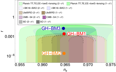
Figure 1: The predicted values of $n_{s},r$ for the three benchmark values from Table 1 are displayed as colored circular dots. The $n_{s}-r$ contours at $1-\sigma$ and $2-\sigma$ C.L. from present and future CMB observations are also displayed in the background. We use deep colored region (located inside) for $95\%$ ($1-\sigma$ C.L.) and light colored region (located outside) for $68\%$ ($2-\sigma$ C.L.) best-fit contours. The bound on $(n_{s},r)$ plane from the Planck 2018 is indicated by green colored region, while bound from combined Planck 2018+Bicep3 (2022)+Keck Array2018 is indicated by blue-shaded region. Other colored regions, with dashed lines as their boundary, indicate contours from future CMB experiments with higher sensitivity - such as LiteBIRD, CMB-S4, and Simons Observatory (SO) Hazumi et al. (2020); Abazajian et al. (2016); Ade et al. (2019).

III.1 Stability analysis

In this subsection, we estimate the maximum permissible value of $y_{\chi}$ and $\lambda_{12}$ (defined in Eq. 4) such that the flatness of the inflationary potential does not get destabilized from the radiative correction emerging from interaction of inflaton with other fields e.g. $\chi$ and $H$. For this, we need to consider Coleman–Weinberg radiative correction at 1-loop order to the inflaton-potential which is  Coleman and Weinberg (1973)

$$V_{{\rm 1-loop}}=\sum_{j}\frac{n_{j}}{64\pi^{2}}(-1)^{2s_{j}}\widetilde{m}_{j}^{4}\left[\ln\left(\frac{\widetilde{m}_{j}^{2}}{\mu^{2}}\right)-c_{j}\right]\,.$$ (15)

Here, $j\equiv H,\chi,\phi$, and $c_{j}=\frac{3}{2}$; $n_{H,\chi}=4$, $n_{\phi}=1$; $s_{H}=0$, $s_{\chi}=1/2$, and $s_{\phi}=0$. In this work, we assume two values of the renormalization scale: $\mu=\phi_{*}$ and $\mu=\phi_{\rm end}$. Meanwhile, the inflaton dependent mass of $H$ and $\chi$ are

$$\widetilde{m}_{\chi}^{2}(\phi)=\left(m_{\chi}+y_{\chi}\phi\right)^{2}\,, \widetilde{m}_{H}^{2}(\phi)=m_{H}^{2}+\lambda_{12}\phi\,.$$ (16)

Now, the first and second derivatives of the Coleman–Weinberg term for $\chi$ and $H$ with respect to $\phi$ are

$$V_{{\rm 1-loop}}^{\prime}=\sum\limits_{j}\frac{n_{j}}{32\pi^{2}}(-1)^{2s_{j}}\widetilde{m}_{j}^{2}\,\left(\widetilde{m}_{j}^{2}\right)^{\prime}\left[\ln\left(\frac{\widetilde{m}_{j}^{2}}{\mu^{2}}\right)-1\right]\,,$$ (17)

$$V_{{\rm 1-loop}}^{\prime\prime}=\sum\limits_{j}\frac{n_{j}}{32\pi^{2}}(-1)^{2s_{j}}\left\{\left[\left(\left(\widetilde{m}_{j}^{2}\right)^{\prime}\right)^{2}+\widetilde{m}_{j}^{2}\left(\widetilde{m}_{j}^{2}\right)^{\prime\prime}\right]\ln\left(\frac{\widetilde{m}_{j}^{2}}{\mu^{2}}\right)-\widetilde{m}_{j}^{2}\left(\widetilde{m}_{j}^{2}\right)^{\prime\prime}\right\}\,.$$ (18)

Using Eq. 16 in Eqs. 17 and 18, we get Coleman–Weinberg correction term for $H$ and $\chi$ as (with $m_{\chi}=m_{H}=0$)

$$\left|V_{{{\rm 1-loop}},H}^{\prime}\right|=\frac{\lambda_{12}^{2}\phi}{8\pi^{2}}\left(\ln\left(\frac{\lambda_{12}\phi}{\mu^{2}}\right)-1\right)\,, \left|V_{{{\rm 1-loop}},\chi}^{\prime}\right|=\frac{\Phi^{3}y_{\chi}^{4}}{4\pi^{2}}\left(1-\ln\left(\frac{\phi^{2}y_{\chi}^{2}}{\mu^{2}}\right)\right)\,,$$ (19)

$$\left|V_{{{\rm 1-loop}},H}^{\prime\prime}\right|=\frac{\lambda_{12}^{2}}{8\pi^{2}}\ln\left(\frac{\lambda_{12}\phi}{\mu^{2}}\right)\,. \left|V_{{{\rm 1-loop}},\chi}^{\prime\prime}\right|=\frac{1}{8\pi^{2}}\left(6\phi^{2}y_{\chi}^{4}\ln\left(\frac{\phi^{2}y_{\chi}^{2}}{\mu^{2}}\right)-2\phi^{2}y_{\chi}^{4}\right)\,.$$ (20)

Let us define tree level potential $V_{\rm tree}(\phi)$ as $V_{\rm tree}(\phi)\equiv V_{\rm GH}(\phi)$. Then

$$V_{\rm tree}^{\prime}(\phi) \equiv V_{\rm GH}^{\prime}(\phi)=-m\,n\,\frac{V_{0}}{\phi}\left(\frac{\phi}{\phi_{0}}\right)^{m}\left(1-\left(\frac{\phi}{{\phi_{0}}}\right)^{m}\right)^{n-1}\,,$$ (21)

$$V_{\rm tree}^{\prime\prime}(\phi) \equiv V_{\rm GH}^{\prime\prime}(\phi)=m\,n\,\frac{V_{0}}{\phi^{2}}\left(\frac{\phi}{\phi_{0}}\right)^{m}\left(1-\left(\frac{\phi}{\phi_{0}}\right)^{m}\right)^{n-2}\left((mn-1)\left(\frac{\phi}{\phi_{0}}\right)^{m}-m+1\right)\,,$$ (22)

Maintaining the stability of the inflation-potential, the maximum allowed value of $\lambda_{12}$ and $y_{\chi}$ can be obtained when all the following conditions are satisfied at $\phi=\mu$

$$\left|V_{{{\rm 1-loop}},H}^{\prime}(\phi=\mu)\right|<V_{\rm tree}^{\prime}(\phi=\mu)\,,\quad \left|V_{{{\rm 1-loop}},\chi}^{\prime}(\phi=\mu)\right|<V_{\rm tree}^{\prime}(\phi=\mu)\,,$$ (23)

$$\left|V_{{{\rm 1-loop}},H}^{\prime\prime}(\phi=\mu)\right|<V_{\rm tree}^{\prime\prime}(\phi=\mu)\,,\quad \left|V_{{{\rm 1-loop}},\chi}^{\prime\prime}(\phi=\mu)\right|<V_{\rm tree}^{\prime\prime}(\phi=\mu)\,.$$ (24)

The permitted upper limit for the couplings $y_{\chi}$ and $\lambda_{12}$ for GH inflationary scenario are listed in Table 3 for $\mu=\phi_{*}$ and $\mu=\phi_{\rm end}$. From this table, we conclude that the permissible upper limit of the couplings are: $y_{\chi}<2.5051\times 10^{-4},<2.7183\times 10^{-4},<3.7039\times 10^{-4}$ and $\lambda_{12}/M_{P}<1.2757\times 10^{-6},<1.2413\times 10^{-7},<1.1649\times 10^{-6}$ for ‘GH-BM1’, ‘GH-BM2’, and ‘GH-BM3’, respectively.

Table 3: Allowed upper limit of $y_{\chi}$ and $\lambda_{12}$ for the benchmark values from Table 1.

Benchmark	stability for $y_{\chi}$		stability for $\lambda_{12}$
	about $\mu=\phi_{*}$	about $\mu=\phi_{\rm end}$	about $\mu=\phi_{*}$	about $\mu=\phi_{\rm end}$
GH-BM1	$y_{\chi}<2.5051\times 10^{-4}$	$y_{\chi}<3.8572\times 10^{-4}$	$\lambda_{12}/M_{P}<1.2757\times 10^{-6}$	$\lambda_{12}/M_{P}<2.1619\times 10^{-6}$
GH-BM2	$y_{\chi}<2.7183\times 10^{-4}$	$y_{\chi}<6.5637\times 10^{-4}$	$\lambda_{12}/M_{P}<1.2413\times 10^{-7}$	$\lambda_{12}/M_{P}<9.9151\times 10^{-7}$
GH-BM3	$y_{\chi}<5.3167\times 10^{-4}$	$y_{\chi}<3.7039\times 10^{-4}$	$\lambda_{12}/M_{P}<5.3244\times 10^{-6}$	$\lambda_{12}/M_{P}<1.1649\times 10^{-6}$

III.2 Reheating era and production of DM

As soon as the slow-roll inflationary phase terminates, inflaton quickly descends to the minimum of the potential and starts coherent oscillations about the minimum of the potential. The minimum of the potential of Eq. 6 is $\phi_{0}$ (for the chosen benchmark values of Table 1) and thus, the physical mass of the inflaton is Enqvist (2012):

$$\frac{m_{\phi}}{M_{P}}=\left(M_{P}^{-2}\,V_{\rm GH}^{\prime\prime}(\phi)|_{\phi=\phi_{0}}\right)^{1/2}\,.$$ (25)

If we define two dimensionless variables $\mathbb{x}=\phi/M_{P}$ and $\mathbb{x}_{0}/M_{P}$, then, we are assuming that expanding the potential $V_{\rm GH}(\mathbb{x})$ about the minimum, $\mathbb{x}_{0}$, we get (for $(\phi-\phi_{0})\ll 1\implies(\mathbb{x}-\mathbb{x}_{0})\ll 1$)

$$V_{\rm GH}(\mathbb{x}-\mathbb{x}_{0})=-m\,V_{0}\,\frac{\left(\mathbb{x}-\mathbb{x}_{0}\right)^{n}}{\mathbb{x}_{0}}+\quad\text{(smaller terms)}\,.$$ (26)

Since we choose $n=2$ for three benchmark values, the energy density of inflaton and pressure, averaging over an oscillating cycle during reheating, behaves as Enqvist (2012) (see also Garcia et al. (2020))

$$\rho_{\phi}\propto\boldsymbol{a}^{-3}\,,\qquad\left<p\right>=0\,.$$ (27)

This oscillating inflaton begins to produce $\chi$ and relativistic Higgs particles $h$ following Eq. 4 and initiates the reheating era. This is a highly adiabatic epoch during which the universe changes from being cold and dominated by the energy density of oscillating inflaton to hot visible universe. The relativistic SM particles produced during reheating era eventually thermalize among themselves and develop the local-thermal fluid of the universe. As a result of that the energy density of radiation, $\rho_{\rm rad}$, and temperature of the universe, $T$, both increase, while $\rho_{\phi}$ decreases. However, $\chi$ being feebly interacting with the SM particles, it may not share the same temperature as that of SM plasma. Sooner, the energy density of oscillating inflaton becomes equal to that of relativistic SM particles. The temperature of the universe at that particular moment is referred to as the reheating temperature, denoted by $T_{\rm rh}$, which can be estimated as Bernal and Xu (2021):

$$T_{\rm rh} =\sqrt{\frac{2}{\pi}}\left(\frac{10}{g_{\star}}\right)^{1/4}\sqrt{M_{P}}\sqrt{\Gamma_{\phi}}\,,$$ (28)

where $g_{\star}=106.75$ is effective number of degrees of freedom of relativistic fluid of the universe and $\Gamma_{\phi}$ is the total decay width of inflaton. At the beginning of reheating era, on the other hand, ${\cal H}$ is greater than $\Gamma_{\phi}$. Then, ${\cal H}$ continues to decrease and it becomes ${\cal H}(T_{\rm rh})\sim\Gamma_{\phi}$, where ${\cal H}(T_{\rm rh})$ is the value of Hubble parameter when the temperature of the universe is $T_{\rm rh}$. After this, $\rho_{\phi}$ is transferred completely and almost immediately to $\rho_{\rm rad}$ and the universe becomes radiation dominated.

It is expected that at the beginning of the reheating epoch, $\rho_{\phi}$ decreases relatively at a faster rate, leading a quick rise of the temperature of the universe. However, after some initial increase of temperature, the Hubble expansion comes into play, causing the temperature to decrease. The maximum attainable temperature during reheating process can be estimated as Giudice et al. (2001); Chung et al. (1999):

$$T_{max}=\Gamma_{\phi}^{1/4}\left(\frac{60}{g_{\star}\,\pi^{2}}\right)^{1/4}\left(\frac{3}{8}\right)^{2/5}{\cal H}_{I}^{1/4}M_{P}^{1/2}\,,$$ (29)

where ${\cal H}_{I}$ is the value of Hubble parameter at the beginning of reheating era when $\rho_{\rm rad}=0$ Giudice et al. (2001) i.e.

$${\cal H}_{I}=\sqrt{\frac{V_{\rm GH}(\phi_{\rm end})}{3M_{P}^{2}}}\,,$$ (30)

i.e. we assume in this work that ${\cal H}_{I}$ is the value Hubble parameter when slow roll inflation ends. $T_{max}>T_{\rm rh}$ indicates that a particle of mass$>T_{\rm rh}$ can still be produced during reheating. Furthermore, in many cases, the amount of DM produced during reheating depends on the ratio $T_{max}/T_{\rm rh}$ (for example, see Refs. Mambrini and Olive (2021); Barman et al. (2022c)). Then, from Eq. 28 and Eq. 29 we get:

$$\frac{T_{max}}{T_{\rm rh}}=\left(\frac{3}{8}\right)^{2/5}\left(\frac{{\cal H}_{I}}{{\cal H}(T_{\rm rh})}\right)^{1/4}\,,$$ (31)

where we have used ${\cal H}(T_{\rm rh})=(2/3)\Gamma_{\phi}$ Bernal and Xu (2021). At $T=T_{\rm rh}$, the universe is radiation dominated and thus

$${\cal H}^{2}(T_{\rm rh})=\frac{1}{3M_{P}^{2}}\left(\frac{\pi^{2}}{30}g_{\star}\,T_{\rm rh}^{4}\right)\,.$$ (32)

Since, we are not considering any variation of $g_{\star}$ during reheating era, $\left(T_{max}/T_{\rm rh}\right)\propto{\cal H}_{I}^{1/4}T_{\rm rh}^{-1/2}$. As a result, for a specific benchmark, ${\cal H}_{I}$ is fixed and, therefore, $\left(T_{max}/T_{\rm rh}\right)$ decreases as $T_{\rm rh}$ increases. In this work, we confine our discussion to perturbative approach of reheating Lozanov (2019). The decay width of inflaton to $\chi$ and $h$ and total decay width of inflaton are Bernal and Xu (2021) (here we neglect the effect of thermal mass Kolb et al. (2003))

$$\Gamma_{\phi\to{hh}}\simeq\frac{\lambda_{12}^{2}}{8\pi\,m_{\phi}}\,,\qquad\Gamma_{\phi\to\chi\chi}\simeq\frac{y_{\chi}^{2}\,m_{\phi}}{8\pi}\,,\qquad\Gamma_{\phi}=\Gamma_{\phi\to{hh}}+\Gamma_{\phi\to\chi\chi}\approx\Gamma_{\phi\to{hh}}\,.$$ (33)

The assumption $\Gamma_{\phi}\sim\Gamma_{\phi\to{hh}}$ is necessary to avoid of DM domination from occurring just after the reheating era. The branching fraction for the production of $\chi$ from the decay-channel then can be defined as

$$\text{Br}=\frac{\Gamma_{\phi\to\chi\chi}}{\Gamma_{\phi\to\chi\chi}+\Gamma_{\phi\to hh}}\simeq\frac{\Gamma_{\phi\to\chi\chi}}{\Gamma_{\phi\to hh}}=m_{\phi}^{2}\left(\frac{y_{\chi}}{\lambda_{12}}\right)^{2}\,.$$ (34)

Now, Table 4 presents the values of $m_{\phi},\Gamma_{\phi},T_{\rm rh}$, and ${\cal H}_{I}$ for the benchmark values mentioned in Table 1. Out of three benchmark values, ${\cal H}_{I}$, and $m_{\phi}$ are the least for ‘GH-BM2’. As a result of this, $T_{\rm rh}/\lambda_{12}$ is the max for this particular benchmark.

Now, using $\Gamma_{\phi}$ from Eq. 33 in Eq. 31, we get

$$\frac{T_{max}}{T_{\rm rh}}\approx 1.67\quantity(\frac{{\cal H}_{I}\,m_{\phi}}{\lambda_{12}^{2}})^{1/4}\,.$$ (35)

Thus, for a specific benchmark value, $T_{max}/T_{\rm rh}$ is highest for the lowest value of $\lambda_{12}$. The lower bound on $\lambda_{12}$ can be obtained from the condition $T_{\rm rh}\gtrsim 4\,\text{Mev}$ (or, ${\cal O}(1\,\text{MeV})$, depending on the theory) which is required for successful Big Bang nucleosynthesis (BBN) and this leads to $\lambda_{12}/M_{P}\gtrsim 5.5449\times 10^{-23}$ (for ‘GH-BM1’), $\gtrsim 4.6885\times 10^{-23}$ (for ‘GH-BM2’), and $\gtrsim 5.1603\times 10^{-23}$ (for ‘GH-BM3’). For these lower limits of $\lambda_{12}$, the highest possible value of $T_{max}/T_{\rm rh}\sim 4.9418\times 10^{8}$ (for ‘GH-BM1’), $\sim 2.4586\times 10^{8}$ (for ‘GH-BM2’), and $\sim 5.2695\times 10^{8}$ (for ‘GH-BM3’). For higher values of $\lambda_{12}$ i.e. for larger values of $T_{\rm rh}$, $T_{max}/T_{\rm rh}$ decreases as mentioned earlier, and it is displayed in Fig. 2. These values can also be approximated using Fig. 2 which shows how $T_{max}/T_{\rm rh}$ declines as $T_{\rm rh}$ increases for two benchmark values – ‘GH-BM2’, and ‘GH-BM3’. Since $T_{max}/T_{\rm rh}$ is almost the same for ‘GH-BM1’ and ‘GH-BM3’, ‘GH-BM1’ is not included in that figure. The gray-colored vertical stripe on the left of the figure indicates bound on the $T_{\rm rh}$ coming from the fact that $T_{\rm rh}\geq 4\,\text{MeV}$ (for successfully occurring of Big Bang nucleosynthesis (BBN)) Giudice et al. (2001). The colored boxes on the lines represent the maximum permissible values of $T_{\rm rh}$ which correspond to the maximum allowable values of $\lambda_{12}$ from Table 3. The colored stripes on the right of the figure indicate that those values of $T_{\rm rh}$ are not allowed from the stability analysis.

Table 4: $m_{\phi},\Gamma_{\phi},T_{\rm rh}$, and ${\cal H}_{I}$ for the benchmark values from Table 1.

Benchmark	$m_{\phi}/M_{P}$	$\Gamma_{\phi}M_{P}$	$T_{\rm rh}/\lambda_{12}$	${\cal H}_{I}/M_{P}$
	(Eq. 25)	(Eq. 33)	(Eq. 28)	(Eq. 30)
GH-BM1	$8.5812\times 10^{-6}$	$4636.73\lambda_{12}^{2}$	$30.0576$	$2.7228\times 10^{-6}$
GH-BM2	$6.1351\times 10^{-6}$	$6485.42\lambda_{12}^{2}$	$35.5482$	$1.6682\times 10^{-7}$
GH-BM3	$7.4321\times 10^{-6}$	$5353.64\lambda_{12}^{2}$	$32.2978$	$3.5200\times 10^{-6}$

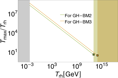
Figure 2: This figure showcases the variation of $T_{max}/T_{\rm rh}$ against $T_{\rm rh}$ for two benchmark values ‘GH-BM2’ and ‘GH-BM3’ from Table 1. The square colored boxes on the lines represent the maximum permissible values of $T_{\rm rh}$ which correspond to the maximum allowable values of $\lambda_{12}$ from Table 3. The vertical stripe on the left of the plot, highlighted in gray, displays lower bound on $T_{\rm rh}$ i.e. $T_{\rm rh}\gtrsim 4\,\text{MeV}$. The colorful stripes on the right side of the plot show that there are no permissible values of $T_{\rm rh}$ based on stability analysis of the corresponding benchmark values.

Next, we consider the production of DM during reheating. If $n_{\chi}$ is the number density of $\chi$, then the conservation equation of the comoving number density, $N_{\chi}$ which is defined as $n_{\chi}\,\boldsymbol{a}^{3}$, is

$$\frac{\text{d}N_{\chi}}{\text{d}t}=\boldsymbol{a}^{3}\,\gamma\,,$$ (36)

in which $t$ is the physical time, and $\gamma\equiv\gamma(t)$ which is the rate of production of $\chi$, has a quartic mass-dimension.

When the temperature of the universe is $T_{max}>T>T_{\rm rh}$, then Bernal and Xu (2021)

$${\cal H}=\frac{\pi}{3}\sqrt{\frac{g_{\star}}{10}}\frac{T^{4}}{M_{P}\,T_{\rm rh}^{2}}\,.$$ (37)

During that period, the energy density of the universe is dominated by $\rho_{\phi}$. Thus, from the first Friedman equation, we get

$$\rho_{\phi}=\frac{\pi^{2}g_{\star}}{30}\frac{T^{8}}{T_{\rm rh}^{4}}\,.$$ (38)

If we combine Eq. 27 with Eq. 38, and then using Eq. 37 into Eq. 36, we obtain

$$\frac{\text{d}N_{\chi}}{\text{d}T}=-\frac{8M_{P}}{\pi}\left(\frac{10}{g_{\star}}\right)^{1/2}\frac{T_{\rm rh}^{10}}{T^{13}}\,\boldsymbol{a}^{3}(T_{\rm rh})\,\gamma\,.$$ (39)

To filter out the effect of the expansion of the universe on the time evolution of $N_{\chi}$ Lisanti (2017), we define DM yield, $Y_{\chi}$, as $Y_{\chi}={n_{\chi}(T)}/{s(T)}$, where $s(T)=\left({2\pi^{2}}/{45}\right)g_{\star,s}\,T^{3}$ and $g_{\star,s}$ refers to the effective number of degrees of freedom contributing to the entropy of the relativistic fluid. We assume that entropy density per comoving volume remains conserved once the reheating era is over. The energy density of $\chi$ continues to decrease with time and finally becomes non-relativistic, contributing to the cold dark matter (CDM) density of the present universe. Present day CDM yield can be calculated as Garrett and Duda (2011)

$$Y_{{\rm CDM},0}=\frac{\Omega_{\rm CDM}\,\rho_{\rm crit}}{s_{0}\,m_{\chi}}=\frac{4.3.\times 10^{-10}}{m_{\chi}}\,,$$ (40)

where $m_{\chi}$ is expressed in  GeV and we have used scaling factor for Hubble expansion rate $h_{\text{CMB}}\approx 0.674$, cold dark matter density of the universe $\Omega_{\rm CDM}=0.12\,h_{\text{CMB}}^{-2}$, present day entropy density $s_{0}=2891.2\,\text{cm}^{-3}$, and critical density of the Universe $\rho_{\rm crit}=1.053\times 10^{-5}\,h_{\text{CMB}}^{2}\,\,\text{GeV}\,\text{cm}^{-3}$ (as we choose $k_{B}=c=1$ unit) from Ref. Workman et al. (2022). Now, we estimate the yield of $\chi$ produced through decay or via scattering, and then compare with $Y_{{\rm CDM},0}$ to determine the extent to which the produced $\chi$ contributes to the total CDM density of the present universe.

III.2.1 Inflaton decay

If $\chi$ is produced exclusively via the decay of inflaton ($\phi\to\bar{\chi}\chi$), then

$$\gamma=2\,\text{Br}\,\Gamma\,\frac{\rho_{\phi}}{m_{\phi}}\,.$$ (41)

When we substitute this in Eq. 39, along with the assumption that the DM yield remains unaltered after the end of reheating to present day, we obtain the expression for the DM Yield from the decay of inflaton as,

$$Y_{\chi,0} =\frac{N_{\chi}(T_{\rm rh})}{s(T_{\rm rh})\,\boldsymbol{a}^{3}(T_{\rm rh})}$$ (42)

$$\simeq\frac{3}{\pi}\frac{g_{\star}}{g_{\star,s}}\sqrt{\frac{10}{g_{\star}}}\frac{M_{P}\,\Gamma}{m_{\phi}\,T_{\rm rh}}\text{Br}=\frac{3}{\pi}\frac{g_{\star}}{g_{\star,s}}\sqrt{\frac{10}{g_{\star}}}\frac{M_{P}}{T_{\rm rh}}\frac{(y_{\chi})^{2}}{8\pi}$$ (43)

$$=1.163\times 10^{-2}M_{P}\frac{y_{\chi}^{2}}{T_{\rm rh}}\,.$$ (44)

Here, we assume $g_{\star,s}=g_{\star}$. Equating Eq. 44 with Eq. 40, we get the condition to generate the complete CDM energy density in terms of the DM mass to be

$$T_{\rm rh}\simeq 6.49\times 10^{25}\,y_{\chi}^{2}\,m_{\chi}\,.$$ (45)

Lines for different values of $y_{\chi}$ from Eq. 45 are shown as discontinuous inclined lines on $(T_{\rm rh},m_{\chi})$ plane in log-log scale in Fig. 3. These lines actually correspond to $\chi$ being produced from the decay of inflaton and also producing the total CDM density of the present-day universe. Fig. 3 actually shows how the permissible region which is shown as white region on $(T_{\rm rh},m_{\chi})$ plane, varies with benchmarks. Bounds on this plane are from: the largest permissible value of $\lambda_{12}$ and $y_{\chi}$ from stability analysis of Table 3 (forest green-colored stripe at the top of the plot and cyan-colored wedge-shaped region at the left-top of the plot for ‘GH-BM1’, while orange-colored stripe at the top of the plot and pink-colored wedge-shaped region at the left-top of the plot for ‘GH-BM2’), BBN temperature: $T_{\rm rh}\gtrsim 4\,\text{MeV}$ (gray colored horizontal stripe at the bottom of the plot), and Ly-$\alpha$ bound from Eq. 47: $T_{\rm rh}\gtrsim(2m_{\phi})/m_{\chi}$ (region shaded with red color for ‘GH-BM1’ and green color for ‘GH-BM2’) and the maximum possible value of $m_{\chi}=m_{\phi}/2$ (vertical stripe at the right, shaded with yellow color for ‘GH-BM1’ and black color for ‘GH-BM2’). The allowed range of $y_{\chi}$ shown by inclined, discontinuous lines passing through the white unshaded region, is $10^{-8}\gtrsim y_{\chi}\gtrsim 10^{-17}$ (for $446.08\,\text{GeV}\lesssim m_{\chi}\lesssim 1.03\times 10^{13}\,\text{GeV}$) for ‘GH-BM1’ and $10^{-8.5}\gtrsim y_{\chi}\gtrsim 10^{-17}$ (for $2783.64\,\text{GeV}\lesssim m_{\chi}\lesssim 7.36\times 10^{12}\,\text{GeV}$) for ‘GH-BM2’. If both $y_{\chi}$ and $m_{\chi}$ fall within these ranges, then it can satisfy two conditions simultaneously: (i) produced solely through the decay of inflation, and (ii) produce the total CDM density of the universe. All the aforementioned bounds vary for three benchmark values mentioned in Table 1. One of the two reason for this variation is different values of $m_{\phi}$, which is already mentioned in Table 4, with $m_{\phi}$ for ‘GH-BM1’$>$ for ‘GH-BM2’. Additionally, the upper limit of the possible value of $\lambda_{12}/M_{P}$ from stability analysis for ‘GH-BM1’$>$‘GH-BM2’. These factor imposes lower limit on $m_{\chi}$ as $2783.64\,\text{GeV}$ for ‘GH-BM2’. However, on this $(T_{\rm rh},m_{\chi})$ plane more stringent bounds can be drawn from gravitino production. Nevertheless, we ignore this bound in our analysis as we do not take supersymmetry into account.

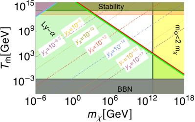
Figure 3: The plot showcases the variation in the permissible region on $(T_{\rm rh},m_{\chi})$ plane as well as allowed range of $y_{\chi}$, specifically for benchmark values ‘GH-BM1’ and ‘GH-BM2’. The region without color on this plane represents the allowed region, and the dashed or dashed-dotted lines that intersect it correspond to Eq. 45 for different values of $y_{\chi}$ satisfying present-day CDM density. The regions shaded in forest green and yellow represent the bounds from the permissible upper bound on $\lambda_{12}$ (from stability analysis) and the maximum possible value of $m_{\chi}$, while the cyan, and red solid lines show the bounds on $y_{\chi}$ from stability analysis, and Ly-$\alpha$ bound on the mass of DM Bernal and Xu (2021) (see also Eq. 47) for ‘GH-BM1’. The same bounds for ‘GH-BM2’ are presented by orange-shaded region, black solid line, purple and green shaded regions. Gray shaded stripe at the bottom is for bound from BBN (i.e. $T_{\rm rh}$ should be $\gtrsim 4\,\text{MeV}$). This figure shows that $y_{\chi}\sim 10^{-8}$ is allowed for ‘GH-BM1’, but not for ‘GH-BM2’.

To derive the Ly-$\alpha$ bound used in Fig. 3 it is assumed that $\chi$ being feebly interacting BSM particle, its momentum only decreases due to red-shift and thus Bernal and Xu (2021)

$$p_{0}=\frac{\boldsymbol{a}_{\rm rh}}{\boldsymbol{a}_{0}}p_{\rm rh}\simeq 3\times 10^{-14}\,\frac{m_{\phi}}{T_{\rm rh}}\,\text{GeV}\,,$$ (46)

where $p_{\rm rh}$ is the momentum of $\chi$ at the time of reheating (i.e. at temperature $T_{\rm rh}$) and $p_{\rm rh}$ is assumed as the initial momentum of the DM particles. Similarly, $p_{0}$, $\boldsymbol{a}_{0}$, and $\boldsymbol{a}_{\rm rh}$ are the momentum, cosmological scale factor today and at the time of reheating, respectively. The maximum possible value of $p_{\rm rh}$ is $p_{\rm rh}=m_{\phi}/2$. If we approximate $p_{0}=m_{\chi}\,v_{\chi}$, where $v_{\chi}$ is the present day velocity of $\chi$ particles, then, using upper bound on $v_{x}/c\lesssim 1.8\times 10^{-8}$ and $m_{c}\gtrsim 3.5\,\text{keV}$ (for further details about bound on the mass of warm dark matter from Ly-$\alpha$ see references within Ghoshal et al. (2022b)) such that $\chi$ as a warm dark matter particle does not negatively impact on structure formation, we can obtain that

$$m_{\chi}\gtrsim 2\frac{m_{\phi}}{T_{\rm rh}}\,,$$ (47)

where $m_{\chi}$ is expressed in  keV.

III.2.2 DM from scattering

In this subsection, we look at three important 2-to-2 scattering mechanisms for DM production: from scattering of non-relativistic inflaton with graviton as the mediator, scattering of SM particles with graviton as mediator, and scattering of SM particles with inflaton as mediator. If $Y_{IS,0}$, $Y_{\text{SM}g,0}$, and $Y_{\text{SM}i,0}$ are respectively the DM yield produced only via those three scattering channels, then Bernal and Xu (2021)

$$Y_{IS,0} \simeq\frac{g_{\star}^{2}}{81920g_{\star,s}}\sqrt{\frac{10}{g_{\star}}}\left(\frac{T_{\rm rh}}{M_{P}}\right)^{3}\left[\left(\frac{T_{max}}{T_{\rm rh}}\right)^{4}-1\right]\frac{m_{\chi}^{2}}{m_{\phi}^{2}}\left(1-\frac{m_{\chi}^{2}}{m_{\phi}^{2}}\right)^{3/2}\,.$$ (48)

$$Y_{\text{SM}g,0} =\begin{cases}\frac{45\,\alpha_{\text{DM}}}{2\pi^{3}g_{\star,s}}\sqrt{\frac{10}{g_{\star}}}\left(\frac{T_{\rm rh}}{M_{P}}\right)^{3},\qquad\text{ for }m_{\chi}\ll T_{\rm rh}\,,\\ \frac{45\,\alpha_{\text{DM}}}{2\pi^{3}g_{\star,s}}\sqrt{\frac{10}{g_{\star}}}\frac{T_{\rm rh}^{7}}{M_{P}^{3}\,m_{\chi}^{4}}\,,\qquad\text{ for }T_{max}\gg m_{\chi}\gg T_{\rm rh}\,.\end{cases}$$ (49)

$$Y_{\text{SM}i,0} \simeq\frac{135\,y^{2}_{\chi}\,\lambda_{12}^{2}}{4\pi^{8}\,g_{\star,s}}\sqrt{\frac{10}{g_{\star}}}\,\frac{M_{P}\,T_{\rm rh}}{m_{\phi}^{4}}\,,\qquad\text{ for }T_{\rm rh}\ll m_{\phi},T_{\rm rh}>T\,.$$ (50)

In Eq. 49, $\alpha_{\text{DM}}=1.1\times 10^{-3}$ Bernal et al. (2018a) and it is related to the coupling of gravitational interaction. In Eq. 48, $Y_{IS,0}$ is increasing function of $T_{\rm rh}$. Now, from the stability analysis of Table 3, maximum permissible value for $T_{\rm rh}$ are

$${T_{\rm rh}}_{\text{, allowable}}=\begin{cases}9.2027\times 10^{13}\,\text{GeV}\,\quad\text{for `GH-BM1'}\,,\\ 1.059\times 10^{13}\,\text{GeV}\,\quad\text{for `GH-BM2'}\,,\\ 9.0297\times 10^{13}\,\text{GeV}\,\quad\text{for `GH-BM3'}\,.\end{cases}$$ (51)

For $T_{\rm rh}\sim{T_{\rm rh}}_{\text{, allowable}}$, $T_{max}/T_{\rm rh}\sim 3.2581$ for ‘GH-BM1’, $\sim 4.7783$ for ‘GH-BM2’, and $\sim 3.5072$ for ‘GH-BM3’. Now, if we choose $T_{\rm rh}\sim{T_{\rm rh}}_{\text{, allowable}}$ from Eq. 51, then, in order to achieve $Y_{IS,0}\sim Y_{{\rm CDM},0}$, it is required that $m_{\chi}$ should be ${m_{\chi}}^{IS,0}$ where

$${m_{\chi}}^{IS,0}\sim\begin{cases}4.1722\times 10^{10}\,\text{GeV}\,\quad\text{for `GH-BM1'}\,,\\ 1.7358\times 10^{11}\,\text{GeV}\,\quad\text{for `GH-BM2'}\,,\\ 3.4993\times 10^{10}\,\text{GeV}\,\quad\text{for `GH-BM3'}\,.\end{cases}$$ (52)

Thus, to achieve comparable values of $Y_{IS,0}$ and $Y_{{\rm CDM},0}$, we need $m_{\chi}>{m_{\chi}}^{IS,0}$ for $T_{\rm rh}<{T_{\rm rh}}_{\text{, allowable}}$. Hence, if $\chi$ is produced exclusively only through the 2-to-2 scattering of inflaton via graviton mediation and contributes completely to the total CDM relic density, the required condition is $m_{\chi}\gtrsim{m_{\chi}}^{IS,0}$ for $T_{\rm rh}\lesssim{T_{\rm rh}}_{\text{, allowable}}$.

For DM production solely through scattering of SM particles with graviton as mediator and for $(m_{\chi}\gg T_{\rm rh})$ and with $T_{\rm rh}\sim{T_{\rm rh}}_{\text{, allowable}}$

$$Y_{\text{SM}g,0}\sim\begin{cases}1.2903\times 10^{-19}\,\quad\text{for `GH-BM1'}\,,\\ 1.9663\times 10^{-22}\,\quad\text{for `GH-BM2'}\,,\\ 1.2189\times 10^{-19}\,\quad\text{for `GH-BM3'}\,.\end{cases}$$ (53)

Consequently, in order to satisfy $Y_{IS,0}\sim Y_{{\rm CDM},0}$, and for $T_{\rm rh}\lesssim{T_{\rm rh}}_{\text{, allowable}}$, it is required that

$$m_{\chi}\gtrsim\begin{cases}3.3326\times 10^{9}\,\text{GeV}\,\quad\text{for `GH-BM1'}\,,\\ 2.1868\times 10^{12}\,\text{GeV}\,\quad\text{for `GH-BM2'}\,,\\ 3.5279\times 10^{9}\,\text{GeV}\,\quad\text{for `GH-BM3'}\,.\end{cases}$$ (54)

Therefore, from Eq. 54 we can deduce that DM particles produced solely though this specific scattering channel (2-to-2 scattering of SM particles with graviton as mediator with $m_{\chi}\ll T_{\rm rh}$) can contribute to the total CDM density, provided that $m_{\chi}$ is very high. However, for $(T_{max}\gg m_{\chi}\gg T_{\rm rh})$ and $Y_{\text{SM}g,0}=Y_{{\rm CDM},0}$, we get

$$\frac{T_{\rm rh}^{\text{SM}g,0}}{\,\text{GeV}}=7.1389\times 10^{12}\,{f}_{T_{\rm rh}}^{-3/4}\,,$$ (55)

where we have assumed $T_{\rm rh}=m_{\chi}\,{f}_{T_{\rm rh}}$, ${f}_{T_{\rm rh}}$ being a fractional number much less than $1$. As the value of ${f}_{T_{\rm rh}}$ decreases, $T_{\rm rh}^{\text{SM}g,0}$ increases. For ${f}_{T_{\rm rh}}\sim 0.6$, $T_{\rm rh}^{\text{SM}g,0}\sim{\cal O}(10^{13})$. However, for $T_{\rm rh}\sim{\cal O}(10^{13})$, $T_{max}/T_{\rm rh}\sim 3$ (see Eq. 51). Therefore, it seems less probable, that satisfying the condition $T_{max}\gg m_{\chi}\gg T_{\rm rh}$, $\chi$ produced through this scattering process (2-to-2 scattering of SM particles with graviton as mediator with $T_{max}\gg m_{\chi}\gg T_{\rm rh}$) contributes $100\%$ of the total CDM density.

Now we consider production of $\chi$ via 2-to-2 scattering of SM particles with inflaton as mediator (along with the constraint $T_{\rm rh}\ll m_{\phi}$). The condition that $Y_{\text{SM}i,0}$ (from Eq. 50) contributes a fraction $f_{\chi}$ ($f_{\chi}$ is a dimensionless fractional number) of total CDM relic density, then we obtain (in  GeV)

$${m_{\chi}}^{\text{SM}i,0}=4.2164\times 10^{-5}\,\frac{m_{\phi}^{4}}{T_{\rm rh},\,M_{P}\,y_{\chi}^{2}\,\lambda_{12}^{2}}\,f_{\chi}\,.$$ (56)

Therefore, as values of $y_{\chi}$ and $\lambda_{12}$ decreases the value of ${m_{\chi}}^{\text{SM}i,0}$ increases. Now, using $T_{\rm rh}=f_{\phi}\,m_{\phi}$ where $f_{\phi}$ is fractional ($\ll 1$) dimensionless number, in Eq. 28, we get (in  GeV)

$${m_{\chi}}^{\text{SM}i,0}=3.2689\times 10^{-7}\,\frac{f_{\chi}}{y_{\chi}^{2}\,f_{\phi}^{3}}\,.$$ (57)

For the maximum permissible values of $y_{\chi}$ (from Table 3) ${m_{\chi}}^{\text{SM}i,0}$ becomes

$${m_{\chi}}^{\text{SM}i,0}=\begin{cases}5.2090\,\frac{f_{\chi}}{f_{\phi}^{3}}\,\text{GeV}\,\quad\text{(for `GH-BM1')}\,,\\ 4.4239\,\frac{f_{\chi}}{f_{\phi}^{3}}\,\text{GeV}\,\quad\text{(for `GH-BM2')}\,,\\ 2.3828\,\frac{f_{\chi}}{f_{\phi}^{3}}\,\text{GeV}\,\quad\text{(for `GH-BM2')}\,.\end{cases}$$ (58)

If $f_{\chi}\sim 1$ and $f_{\phi}\sim 10^{-2}$, then for ${m_{\chi}}^{\text{SM}i,0}\sim{\cal O}(10^{8})\,\text{GeV}$, $\chi$ produced through this scattering channel (2-to-2 scattering of SM particles with inflaton as mediator with $T_{\rm rh}\ll m_{\phi}$) can contribute total CDM relic density.

Therefore, if $\chi$ is produced solely via either of the three scattering processes we have considered (i.e. 2-to-2 scattering of non-relativistic inflaton with graviton as the mediator,2-to-2 scattering of SM particles with graviton as mediator with $m_{\chi}\ll T_{\rm rh}$, and 2-to-2 scattering of SM particles with inflaton as mediator with $T_{\rm rh}\ll m_{\phi}$), for GH inflation, then produced $\chi$ can contribute up to $100\%$ of the total CDM relic density of the present universe.

IV Non-minimal inflation

The most recent Planck 2018+Bicep+Keck Array combined data has ruled out various extremely popular single-field cosmic inflation models, including those have simple form of potentials or are based on well-established theories such as Higgs Inflation, Natural Inflation, chaotic inflation with power law potential, Coleman-Weinberg inflation, and so on. These models mostly predict high values of $r$ (along with high or low values of $n_{s}$). In order to be consistent with the observations, one of the possible solutions (for other possibilities, see Akrami et al. (2020)) is to consider a non-minimal coupling between the inflaton and gravity sectors. When the inflaton is non-minimally coupled to gravity, the action for slow roll inflation can be written as Nozari and Sadatian (2008); Cheong et al. (2022); Kodama and Takahashi (2022)

$${\cal S}^{JF}\supset\int\text{d}^{4}x\sqrt{-g^{JF}}\left(\frac{1}{2}M_{P}^{2}\,\Omega^{2}(\varphi)\,{\cal R}^{JF}+\frac{1}{2}\left(\partial\varphi\right)^{2}-V^{JF}(\varphi)\right)\,,$$ (59)

where the superscript $JF$ indicates that the corresponding quantity is defined in Jordan frame, $\varphi$ is the inflaton in the Jordan frame. $\Omega^{2}(\varphi)\equiv\Omega^{2}\neq 0$ and $\Omega^{2}(v_{\rm inf})=M_{P}^{2}$, where $v_{\rm inf}$ is the vacuum expectation value of inflation at the end of inflation. The last condition ensures ordinary Einstein gravity at low energy scale Watanabe and Komatsu (2007) (also Kannike et al. (2015)). Now, let us define

$$\Omega^{2}(\varphi)=1+\frac{F(\varphi)}{M_{P}^{2}}\,.$$ (60)

Gravity sector is canonical in Einstein frame. To obtain the space-time metric in Einstein frame, we need to perform Weyl transformation as

$$g^{E}_{\mu\nu}=\Omega^{2}\,g^{JF}_{\mu\nu}\,.$$ (61)

The symbols with superscript $E$ symbolize the corresponding quantity is defined in Einstein frame. Now, in Einstein frame, the action can be written in the following form

$${\cal S}^{E}\supset\int\text{d}^{4}x\sqrt{-g^{E}}\left(\frac{1}{2}M_{P}^{2}\,{\cal R}^{E}+\frac{1}{2}\left(\partial\phi\right)^{2}-V^{E}(\phi)\right)\,,$$ (62)

where $\phi$ is the inflaton in Einstein frame which is introduced so that the kinetic energy of inflaton in the action in Eq. 62 is canonical. Actually, $\phi$ depends on $\varphi$ as

$$\frac{d\phi}{d\varphi}=\sqrt{\Pi(\varphi)}\,.$$ (63)

Here, Shaposhnikov et al. (2020)

$$\Pi(\varphi)\equiv\frac{1}{\Omega^{2}}+\kappa\,\frac{3}{2M_{P}^{2}}\frac{1}{\Omega^{4}}\left(\frac{\text{d}F(\varphi)}{\text{d}\varphi}\right)^{2}, \kappa=1 \,\text{(Metric formalism) }\,.$$ (64)

Moreover, the potential of the inflaton in Einstein frame is

$$V^{E}(\phi)=\frac{V^{JF}\left(\varphi(\phi)\right)}{\Omega^{4}\left(\varphi(\phi)\right)}\,.$$ (65)

For slow roll inflation in Einstein frame, the first two slow roll parameters are defined as Oda et al. (2018); Järv et al. (2017); Kodama and Takahashi (2022)

$$\epsilon_{V}^{E}=\frac{M_{P}^{2}}{2}\quantity(\frac{\text{d}\ln[V^{E}]}{\text{d}\varphi}\frac{\text{d}\varphi}{\text{d}\phi})^{2}\,,$$ (66)

$$\eta_{V}^{E}=M_{P}^{2}\quantity(\frac{1}{V^{E}}\frac{\text{d}^{2}V^{E}}{\text{d}\varphi^{2}}\left(\frac{\text{d}\varphi}{\text{d}\phi}\right)^{2}-\frac{\text{d}\ln[V^{E}]}{\text{d}\varphi}\frac{\text{d}^{2}\phi}{\text{d}\varphi^{2}}\left(\frac{\text{d}\varphi}{\text{d}\phi}\right)^{3})\,.$$ (67)

The amplitude of the curvature perturbation $A_{s}$ is given by

$$A_{s}\approx\frac{1}{24\pi^{2}}\frac{1}{M_{P}^{4}}\left.\frac{V^{E}}{\epsilon_{V}^{E}}\right|_{k=k_{\star}},$$ (68)

where $k_{\star}$ is the pivot scale at which CMB measurements are done. The total number of e-folds during which the slow roll inflation happens, is defined as Oda et al. (2018)

$${\cal N}_{\text{CMB}}=\frac{1}{M_{P}}\int_{\varphi_{{\rm end}}}^{\varphi_{*}}\text{d}\varphi\;\frac{1}{\sqrt{2\,\epsilon_{V}^{E}}}\frac{\text{d}\phi}{\text{d}\varphi},$$ (69)

where $\varphi_{*}$ is the value of inflaton corresponding to $k_{\star}$ and $\varphi_{{\rm end}}$ is the value of inflaton corresponding to the end of inflation. The scalar spectral index $n_{s}$, the tensor-to-scalar ratio $r$ are

$$n_{s}(\varphi_{*})=1-6\,\epsilon_{V}^{E}(\varphi_{*})\,+\,2\,\eta_{V}^{E}(\varphi_{*}),\;\; r(\varphi_{*})=16\,\epsilon_{V}^{E}(\varphi_{*}),\;\;$$ (70)

Current CMB constraints on $A_{s}$, $n_{s}$, and $r$ are already mentioned in Table 2. In the following sections, we discuss three inflationary scenarios where inflaton is non-minimally connected to gravity.

V Non-minimal Coleman-Weinberg inflation

Any fundamental BSM scalar particle receives quantum corrections arising either due to self-interactions of gauge or Yukawa interactions present in the theory. Such quantum corrections (mostly coming from dimension-4 operators due to renormalizalibity conditions) are logarithimic in nature. If such a potential is assumed to drive the inflation the renormalization group (RG) improved effective inflationary potential which is typically given by Racioppi (2017); Kannike et al. (2016, 2014); Bostan (2020)

$$V^{JF}(\varphi)=\frac{\lambda_{\rm eff}(\varphi)}{4}\,\varphi^{4}+\Lambda_{CW}$$ (71)

where $\Lambda_{CW}$ is a constant having quartic mass dimension. $\lambda_{\rm eff}(\varphi)$ can be written approximately as

$$\lambda_{\rm eff}(\varphi)=\lambda_{\rm eff}({\cal Q})+\beta_{\rm eff}({\cal Q})\,f(\log[\varphi/{\cal Q}])$$ (72)

Here, ${\cal Q}$ is the renormalization scale such that the beta function $\beta_{\rm eff}({\cal Q})=\frac{\partial}{\partial\log[{\cal Q}]}\lambda_{\rm eff}({\cal Q})$ and $f(\log[\varphi/{\cal Q}])$ is a polynomial function of $\log(\varphi/{\cal Q})$. Considering the 1-loop correction and adjusting $\Lambda_{CW}$ from the condition $V^{JF}(\varphi={\cal Q})=0$, the effective potential in Jordan frame Martin et al. (2014)

$$V^{JF}(\varphi)=V_{\text{NM-CW}}(\varphi)=\frac{A{\cal Q}^{4}}{4}+A\varphi^{4}\left[\log\left(\frac{\varphi}{{\cal Q}}\right)-\frac{1}{4}\right]\,.$$ (73)

Here $\Lambda_{CW}=A\,{\cal Q}^{4}/4$. ${\cal Q}$ has the dimension of mass and ${\cal Q}=\left<\varphi\right>$ is the renormalization scale with $V(\varphi={\cal Q})=V^{\prime}(\varphi={\cal Q})=0$. $A$ is dimensionless and $A=A({\cal Q})$ is determined by the beta function of the scalar-quartic-coupling with inflaton. Now, we are assuming non-minimal coupling to the gravity of the following form Maji and Shafi (2023)

$$\Omega^{2}(\varphi)=1+\xi\frac{\varphi^{2}-{\cal Q}^{2}}{M_{P}^{2}}\,,$$ (74)

and then the inflaton transforms from Jordan to Einstein as

$$\frac{\text{d}\phi}{\text{d}\varphi}=\sqrt{\frac{\xi(6\xi+1)\varphi^{2}M_{P}^{2}-\xi{\cal Q}^{2}M_{P}^{2}+M_{P}^{4}}{\left(M_{P}^{2}+\xi(\varphi^{2}-{\cal Q}^{2})\right){}^{2}}\,,}$$ (75)

thus the potential of this inflationary scenario (non-minimal Coleman Weinberg, abbreviated as NM-CW inflation) transforms in Einstein frame as

$$V^{E}(\varphi)\equiv V_{\text{NM-CW}}^{E}(\varphi)=\frac{\frac{A{\cal Q}^{4}}{4}+A\varphi^{4}\left[\log\left(\frac{\varphi}{{\cal Q}}\right)-\frac{1}{4}\right]}{\left(1+\xi\frac{\varphi^{2}-{\cal Q}^{2}}{M_{P}^{2}}\right)^{2}}\,.$$ (76)

This NM-CW scenario involves inflation beginning near $\varphi=0$ and then the inflaton travels towards $\varphi_{\rm min}$, the minimum of the potential of Eq. 76. The benchmark values of the above-mentioned inflationary scenario are mentioned in Table 5 and the $n_{s}-r$ predictions for the two benchmark values from Table 5 are shown in Fig. 4. The predicted value $r$ for benchmark ‘(m)NM-CW-1’ and ‘(m)NM-CW-2’ fall within $1-\sigma$ and $2-\sigma$ best-fit contour of Planck2018+Bicep3 (2022)+Keck Array2018 data and SO analysis, respectively.

Table 5: Benchmark values for NM-CW inflationary model in metric formalism (for ${\cal N}_{\text{CMB}}\approx 60$).

Benchmark	${\cal Q}/M_{P}$	$\xi$	$\varphi_{*}/M_{P}$	$\varphi_{\rm end}/M_{P}$	$n_{s}$	$r\times 10^{2}$	$A$
(m)NM-CW1	$52$	$-0.002$	$39.0185$	$50.7913$	$0.964728$	$1.5708$	$\ 9.4735\times 10^{-15}$
(m)NM-CW2	$500$	$-0.003$	$488.912$	$499.642$	$0.964318$	$0.3$	$1.8083\times 10^{-15}$

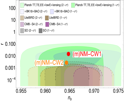
Figure 4: The predicted values of $n_{s},r$ for the two benchmark values from Table 5 are displayed as colored circular dots. In addition, this figure also displays $2-\sigma$ and $1-\sigma$ $(n_{s},r)$ best-fit contours from the Planck 2018+Bicep, as well as additional upcoming CMB observations mentioned ealier in Fig. 1.

V.1 Stability

Following Sec. III.1, the objective of this section is to determine the upper limit of $y_{\chi}$ and $\lambda_{12}$ in Einstein frame to ensure that the stability of the potential of Eq. 76 is not compromised. The background-field dependent mass of $H$ and $\chi$ are given by:

$$\widetilde{m}_{\chi}^{2}(\phi)=\left(m_{\chi}+y_{\chi}\phi\right)^{2}\,, \widetilde{m}_{H}^{2}(\phi)=m_{H}^{2}+\lambda_{12}\phi\,.$$ (77)

Similarly, the first and second derivative of Coleman–Weinberg correction term for $H$ and $\chi$ are (with $m_{\chi}=m_{H}=0$)

$$\left|V_{{{\rm 1-loop}},H}^{\prime}\right|=\frac{\lambda_{12}^{2}\phi}{8\pi^{2}}\left(\ln\left(\frac{\lambda_{12}\phi}{\mu^{2}}\right)-1\right)\,, \left|V_{{{\rm 1-loop}},\chi}^{\prime}\right|=\frac{\Phi^{3}y_{\chi}^{4}}{4\pi^{2}}\left(1-\ln\left(\frac{\phi^{2}y_{\chi}^{2}}{\mu^{2}}\right)\right)\,,$$ (78)

$$\left|V_{{{\rm 1-loop}},H}^{\prime\prime}\right|=\frac{\lambda_{12}^{2}}{8\pi^{2}}\ln\left(\frac{\lambda_{12}\phi}{\mu^{2}}\right)\,. \left|V_{{{\rm 1-loop}},\chi}^{\prime\prime}\right|=\frac{1}{8\pi^{2}}\left(6\phi^{2}y_{\chi}^{4}\ln\left(\frac{\phi^{2}y_{\chi}^{2}}{\mu^{2}}\right)-2\phi^{2}y_{\chi}^{4}\right)\,.$$ (79)

By integrating Eq. 75, and using the resulting function $\phi(\varphi)$, Eqs. 78 and 79 can be expressed as a function of $\varphi$. However, in NM-CW Inflation, tree-level potential and its first and second derivative in Einstein frame are

$$V_{tree}(\varphi)=V_{\text{NM-CW}}^{E}(\varphi)=\frac{\frac{A{\cal Q}^{4}}{4}+A\varphi^{4}\left[\log\left(\frac{\varphi}{{\cal Q}}\right)-\frac{1}{4}\right]}{\left(1+\xi\frac{\varphi^{2}-{\cal Q}^{2}}{M_{P}^{2}}\right)^{2}}\,,$$ (80)

$$V^{\prime}_{tree}(\varphi)=\quantity(\frac{\text{d}V_{\text{NM-CW}}^{E}}{\text{d}\varphi}\frac{\text{d}\varphi}{\text{d}\phi})\,,$$ (81)

$$V^{\prime\prime}_{tree}(\varphi)=\frac{\text{d}}{\text{d}\varphi}\quantity(\frac{\text{d}V_{\text{NM-CW}}^{E}}{\text{d}\varphi}\frac{\text{d}\varphi}{\text{d}\phi})\frac{\text{d}\varphi}{\text{d}\phi}\,.$$ (82)

To obtain the upper limit of $y_{\chi}$ and $\lambda_{12}$, we need to satisfy

$$\left|V_{{{\rm 1-loop}},H}^{\prime}(\varphi=\mu)\right|<V_{\rm tree}^{\prime}(\varphi=\mu)\,,\quad \left|V_{{{\rm 1-loop}},\chi}^{\prime}(\varphi=\mu)\right|<V_{\rm tree}^{\prime}(\varphi=\mu)\,,$$ (83)

$$\left|V_{{{\rm 1-loop}},H}^{\prime\prime}(\varphi=\mu)\right|<V_{\rm tree}^{\prime\prime}(\varphi=\mu)\,,\quad \left|V_{{{\rm 1-loop}},\chi}^{\prime\prime}(\varphi=\mu)\right|<V_{\rm tree}^{\prime\prime}(\varphi=\mu)\,.$$ (84)

The permissible upper limit of $y_{\chi}$ and $\lambda_{12}$ for NM-CW inflationary scenario is listed in Table 6 for $\mu=\varphi_{*}$ and $\mu=\varphi_{\rm end}$. From this table, we conclude that the permissible upper limit of the couplings $y_{\chi}<3.0671\times 10^{-4}$, $\lambda_{12}/M_{P}<2.3304\times 10^{-6}$ for ‘(m)NM-CW-1’, and $y_{\chi}<1.1517\times 10^{-4}$, $\lambda_{12}/M_{P}<4.7788\times 10^{-7}$ for ‘(m)NM-CW-2’.

Table 6: Allowed range of $y_{\chi}$ and $\lambda_{12}$ for the benchmark values from Table 5.

Benchmark	stability for $y_{\chi}$		stability for $\lambda_{12}$
	about $\phi_{*}$	about $\phi_{\rm end}$	about $\phi_{*}$	about $\phi_{\rm end}$
(m)NM-CW-1	$y_{\chi}<3.0956\times 10^{-4}$	$y_{\chi}<3.0671\times 10^{-4}$	$\lambda_{12}/M_{P}<2.3304\times 10^{-6}$	$\lambda_{12}/M_{P}<3.3614\times 10^{-6}$
(m)NM-CW-2	$y_{\chi}<1.1517\times 10^{-4}$	$y_{\chi}<2.2136\times 10^{-4}$	$\lambda_{12}/M_{P}<4.7788\times 10^{-7}$	$\lambda_{12}/M_{P}<2.0868\times 10^{-6}$

V.2 Reheating and DM from decay

As discussed earlier, the potential of Eq. 76 has a minimum at $\varphi={\cal Q}$. In this work, we assume that $V_{\text{NM-CW}}^{E}(\phi)$ can be approximated around the minimum as $V_{\text{NM-CW}}^{E}(\phi)\sim\phi^{2}$ such that during reheating, inflaton oscillates about a quadratic minimum at leading order. Moreover, similar to GH inflation, we utilize the perturbative reheating technique and particle creation in the Einstein frame, as described by Eq. 4. In this inflationary scenario, mass of the inflaton, $m_{\phi}$ is defined as

$$\frac{m_{\phi}}{M_{P}}=\left(\frac{1}{M_{P}^{2}}\left.\frac{\text{d}^{2}V^{E}(\phi)}{\text{d}\phi^{2}}\right|_{\phi=\phi_{\rm min}}\right)^{1/2}\,.$$ (85)

Similarly, $\Gamma_{\phi}$, $T_{\rm rh}$, and ${\cal H}_{I}$ for the benchmark values from Table 5 are listed in Table 7. The benchmark ‘(m)NM-CW-2’ has a higher value of $m_{\phi}$ and a smaller value of ${\cal H}_{I}$ compared to the benchmark ‘(m)NM-CW-1’. Nevertheless, the values of $m_{\phi}$, and ${\cal H}_{I}$ of the two benchmarks are almost identical.

The variation of $T_{max}/T_{\rm rh}$ vs. $T_{\rm rh}$ for NM-CW is illustrated in Fig. 5- the solid line is for ‘(m)NM-CW-1’. The gray-colored vertical stripe on the left of the figure shows a limit on $T_{\rm rh}$ due to the requirement that it must be $\geq 4\,\text{MeV}$. On the right-hand side of the figure, there is a colored stripe that signifies that those $T_{\rm rh}$ values are not permitted based on the stability analysis from Table 6. The maximum value of $T_{max}/T_{\rm rh}$ is $5.4145\times 10^{8}$ for ‘(m)NM-CW-1’ (and maximum value of $T_{max}/T_{\rm rh}\sim 5.0616\times 10^{8}$ for ‘(m)NM-CW-2’ at $T_{\rm rh}\sim 4\,\text{MeV}$). Furthermore, lower bound on $T_{\rm rh}$ leads to establishing the minimum permissible value of $\lambda_{12}$ which are $\lambda_{12}/M_{P}\gtrsim 5.9284\times 10^{-23}$ for ‘(m)NM-CW-1’, and $\lambda_{12}/M_{P}\gtrsim 6.3255\times 10^{-23}$ for ‘(m)NM-CW-2’.

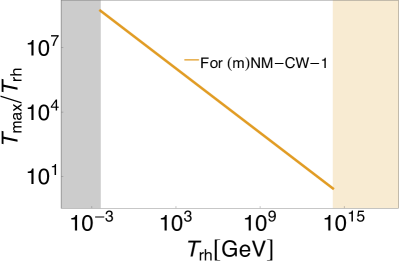
Figure 5: This figure showcases the variation of $T_{max}/T_{\rm rh}$ against $T_{\rm rh}$ for benchmark value ‘(m)NM-CW-1’ from Table 5. The vertical stripe on the left of the plot, highlighted in gray, displays the lower bound on $T_{\rm rh}$ i.e. $T_{\rm rh}\gtrsim 4\,\text{MeV}$. The colorful stripe on the right of the plot shows that there is no permissible value of $T_{\rm rh}$ based on stability analysis of the corresponding benchmark value from Table 6.

Table 7: $m_{\varphi},\Gamma_{\varphi},T_{\rm rh}$, and ${\cal H}_{I}$ for the benchmark values from Table 5.

Benchmark	$m_{\phi}/M_{P}$	$\Gamma_{\phi}M_{P}$	$T_{\rm rh}/\lambda_{12}$	${\cal H}_{I}/M_{P}$
	(Eq. (85))	(Eq. (33))	(Eq. (28))	(Eq. 30)
(m)NM-CW-1	$9.8092\times 10^{-6}$	$4056.25\,\lambda_{12}^{2}$	$28.1132$	$3.9237\times 10^{-6}$
(m)NM-CW-2	$1.1167\times 10^{-5}$	$3562.97\,\lambda_{12}^{2}$	$26.3484$	$2.9965\times 10^{-6}$

Similarly, Fig. 6 shows $(T_{\rm rh},m_{\chi})$ plane for NM-CW inflation, particularly for benchmark ‘(m)NM-CW-1’. The discontinuous lines correspond to Eq. 45. The bounds on this plane is similar to Fig. 3: the largest permissible value of $\lambda_{12}$ and $y_{\chi}$ from stability analysis of Table 6 (orange-colored horizontal stripe at the top of the plot and pink-colored wedge-shaped region at the left-top corner of the plot), BBN temperature: $T_{\rm rh}\gtrsim 4\,\text{MeV}$ (gray colored horizontal stripe at the bottom of the plot), and Ly-$\alpha$ bound from Eq. 47: $T_{\rm rh}\gtrsim(2m_{\phi})/m_{\chi}$ (region shaded with green color) and maximum possible value of $m_{\chi}=m_{\phi}/2$ (vertical stripe at the right, shaded with yellow color). The unshaded region is allowed on $(T_{\rm rh},m_{\chi})$ plane and thus if $10^{-8}\gtrsim y_{\chi}\gtrsim 10^{-17.5}$ ($299.501\,\text{GeV}\lesssim m_{\chi}\lesssim 1.1771\times 10^{13}\,\text{GeV}$), then $\chi$ produced only via the decay of inflaton for the benchmark ‘(m)NM-CW-1’ in NM-CW inflationary scenario can contribute up to $100\%$ of the entire CDM relic density of the present universe. Since, $m_{\phi}$ and ${\cal H}_{I}$ are almost similar for ‘(m)NM-CW-1’ and ‘(m)NM-CW-2’ (see Table 7), Ly$-\alpha$ and $m_{\chi}\lesssim m_{\phi}/2$ are almost similar for both benchmarks. However, significant difference on the allowed region on $(T_{\rm rh},m_{\chi})$ for the two benchmark values comes the maximum permissible value of $T_{\rm rh}$ from stability analysis of Table 6. As a result, the permitted range of $m_{\chi}$ for ‘(m)NM-CW-2’ is almost similar - $1773.36\,\text{GeV}\lesssim m_{\chi}\lesssim 1.3401\times 10^{13}\,\text{GeV}$.

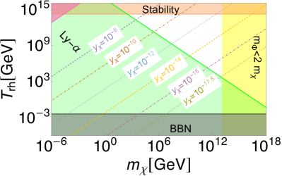
Figure 6: The region without any color on $(T_{\rm rh},m_{\chi})$ plane, depicted on log-log scale, indicates the allowed region for the benchmark value ‘(m)NM-CW-1’ from Table 5. The dashed or dashed-dotted lines that intersect the white region correspond to Eq. 45 for various values of $y_{\chi}$ that satisfy present-day CDM relic density. The colored regions on this plane represent various bounds – stability analysis: the maximum allowed value of $T_{\rm rh}$ from the upper limit of $\lambda_{12}$ from Table 6 (orange horizontal stripe at the top) and the maximum allowed value of $y_{\chi}$ from Table 6 (pink-colored wedge-shaped region at the top-left), from Ly-$\alpha$ bound on the mass of DM Eq. 47: green-colored region, and $m_{\chi}\lesssim m_{\phi}/2$: yellow colored vertical stripe on the right. The gray colored stripe at the bottom depicts that $T_{\rm rh}$ should be $\gtrsim 4\,\text{MeV}$.

V.3 DM fromm scattering

Similar to GH inflationary scenario, there is an upper limit on $\lambda_{12}$ from the stability analysis in this case (NM-CWinflation). Therefore, upper limit on $T_{\rm rh}$ from stability analysis

$${T_{\rm rh}}_{,\text{allowable}}=\begin{cases}1.5724\times 10^{14}\,\text{GeV}\,\quad\text{for `(m)NM-CW-1'}\,,\\ 3.0219\times 10^{13}\,\text{GeV}\,\quad\text{for `(m)NM-CW-2'}\,.\end{cases}$$ (86)

And for such maximum possible values of $T_{\rm rh}$, $T_{max}/{T_{\rm rh}}_{,\text{allowable}}>1$ is maintained. Now, for $T_{\rm rh}\sim{T_{\rm rh}}_{,\text{allowable}}$, and the condition $Y_{IS,0}\sim Y_{{\rm CDM},0}$ (from Eqs. 48 and 45), the value of $m_{\chi}$ is

$${m_{\chi}}^{IS,0}\sim\begin{cases}3.3884\times 10^{10}\,\text{GeV}\,\quad\text{for `(m)NM-CW-1'}\,,\\ 6.9634\times 10^{10}\,\text{GeV}\,\quad\text{for `(m)NM-CW-2'}\,.\end{cases}$$ (87)

Therefore, for NM-CW, the required condition to make $Y_{IS,0}\sim Y_{{\rm CDM},0}$ is $m_{\chi}\gtrsim{m_{\chi}}^{IS,0}$ for $T_{\rm rh}\lesssim{T_{\rm rh}}_{,\text{allowable}}$.

In the scenario where DM particles are produced through the scattering process involving SM particles and the mediator being a graviton (with $m_{\chi}\ll T_{\rm rh}$) (Eq. 49), assuming $T_{\rm rh}\sim{T_{\rm rh}}_{,\text{allowable}}$, we obtain

$$Y_{\text{SM}g,0}=\begin{cases}6.4357\times 10^{-19}\,\quad\text{(for `(m)NM-CW-1')}\,,\\ 4.5687\times 10^{-21}\,\text{GeV}\,\quad\text{(for `(m)NM-CW-2')}\,.\end{cases}$$ (88)

And thus to make $Y_{\text{SM}g,0}\sim Y_{{\rm CDM},0}$ (from Eq. 40), we get

$$m_{\chi}\sim\begin{cases}6.6815\times 10^{8}\,\text{GeV}\,\quad\text{(for `(m)NM-CW-1')}\,,\\ 9.4119\times 10^{10}\,\text{GeV}\,\quad\text{(for `(m)NM-CW-2')}\,.\end{cases}$$ (89)

However, it appears that the conclusion for NM-CW is similar to GH inflation for 2-to-2 scattering of SM particles with graviton as mediator with $T_{max}\gg m_{\chi}\gg T_{\rm rh}$following Eq. 55. This is because $T_{max}/T_{\rm rh}\sim 30$ for $T_{\rm rh}\sim 10^{12}\,\text{GeV}$ and $T_{max}/{T_{\rm rh}}_{,\text{allowable}}\sim 3$ for ‘(m)NM-CW-1’ and $T_{max}/{T_{\rm rh}}_{,\text{allowable}}\sim 10$ for ‘(m)NM-CW-2’ (see Eq. 86).

For the production of $\chi$ via 2-to-2 scattering of SM particles with inflaton as mediator (along with the constraint $T_{\rm rh}\ll m_{\phi}$), the condition that $Y_{\text{SM}i,0}$ contributes $f_{\chi}$ fraction of total CDM relic density (Eq. 57) along with the maximum permissible values of $y_{\chi}$ (from Table 6)

$${m_{\chi}}^{\text{SM}i,0}=\begin{cases}3.4749\,\frac{f_{\chi}}{f_{\phi}^{3}}\,\text{GeV}\,\quad\text{(for `(m)NM-CW-1')}\,,\\ 24.6447\,\frac{f_{\chi}}{f_{\phi}^{3}}\,\text{GeV}\,\quad\text{(for `(m)NM-CW-2')}\,.\end{cases}$$ (90)

Therefore, just like in GH inflationary scenario, if $f_{\chi}/f_{\phi}^{3}\sim 1$, then $m_{\chi}\sim{\cal O}(10)\,\text{GeV}$, while for $f_{\chi}/f_{\phi}^{3}\sim 10^{8}$, $m_{\chi}\sim{\cal O}(10^{8}-10^{9})\,\text{GeV}$ is required.

VI Discussion and Conclusion

In this study, we considered two distinct slow roll single-field inflationary scenarios: GH with inflaton minimally coupled to gravity and NM-CW with inflaton non-minimally coupled to gravity and suggested production of a non-thermal vector-like fermionic particle $\chi$ during reheating era. For each inflationary model, we considered a set of benchmark values and for those set of benchmark values, we explored the permissible parameter space encompassing $y_{\chi}$, $m_{\chi}$, assuming that $\chi$ is a potential candidate for the CDM of the present universe. Salient features of our findings are as follows:

• For our chosen benchmarks, we found that $r$ can be as small as $2.69\times 10^{-6}$ for small-field GH inflationary scenario (see Table 1), and this predicted value fits inside $1-\sigma$ contour on $(n_{s},r)$ plane of Planck2018+Bicep3+Keck Array2018 as well as upcoming SO experiment. On the other hand, the lowest value of $r$ we found for NM-CW inflation is $\sim 3\times 10^{-3}$, which can be corroborated by upcoming SO (see Table 5).

• Using stability analysis and bound from BBN temperature, we computed the permissible upper limit for the coupling $y_{\chi}$ and permissible range for $\lambda_{12}$ (defined in Eq. 4) for GH and NM-CW inflation and found $y_{\chi}<{\cal O}\quantity(10^{-4})$ and ${\cal O}(10^{-5})\lesssim\lambda_{12}\lesssim{\cal O}(10^{11})$ (in  GeV)(see Tables 3 and 6), and these limits varies with various benchmarks as well as inflationary models. The highest value for $y_{\chi}$ is found for ‘GH-BM3’ and largest allowed range of $\lambda_{12}$ for the ‘GH-BM2’ among all chosen benchmarks in both inflationary scenarios.

• From Tables 4 and 7, we infer that the value of $m_{\phi}$ is subject to alteration depending on benchmarks (and thus with inflationary parameters, including $r$) and inflationary scenarios, being highest ($\sim 2.6801\times 10^{13}\,\text{GeV}$) for ‘(m)NM-CW-2’ and lowest for ‘GH-BM2’ ($\sim 1.4724\times 10^{13}\,\text{GeV}$), consequently affecting $T_{\rm rh}$, Ly-$\alpha$ bound and maximum possible value of $m_{\chi}$.

• Figs. 2 and 5 illustrates the variation of $T_{max}/T_{\rm rh}$ against $T_{\rm rh}$ with the highest value of $T_{max}/T_{\rm rh}\sim{\cal O}\quantity(10^{8})$ at $T_{\rm rh}\sim 4\,\text{MeV}$. However, $T_{max}/T_{\rm rh}$ changes based on chosen benchmarks and thus depends on inflationary parameters, e.g. $n_{s}$, $r$, etc.

• Ensuring that $\chi$ is produced only through inflaton decay and contributes $100\%$ of the total relic density of CDM of the present universe, Figs. 3 and 6 demonstrates that the allowed range of $y_{\chi}$ is $10^{-8}\gtrsim y_{\chi}\gtrsim 10^{-17}$ for both GH and NM-CW inflationary scenarios. However, the allowed space on the $(T_{\rm rh},m_{\chi})$ plane, which determines the allowed range of $y_{\chi}$, varies with benchmark values (for example, see Fig. 3) and thus depends on inflationary parameters.

• Assuming that $\chi$ is produced via 2-to-2 scattering channels involving SM particles with $m_{\chi}\ll T_{\rm rh}$ or non-relativistic inflaton (both processes are mediated by graviton) or through 2-to-2 scattering of SM particles with inflaton as mediator with $T_{\rm rh}\ll m_{\phi}$, it was found that the individual contributions from these scattering channels for each inflationary scenario can account for $100\%$ of the total CDM yield of the present universe if $m_{\chi}\gtrsim{\cal O}(10^{10})\,\text{GeV}$ (see Eqs. 52 and 87) and $m_{\chi}\gtrsim{\cal O}(10^{9})\,\text{GeV}$ (see Eqs. 54 and 89) and $m_{\chi}\gtrsim{\cal O}(10^{8})\,\text{GeV}$ (for $T_{\rm rh}\sim 10^{-2}m_{\phi}$, see Eqs. 58 and 90) , respectively. However, depending on the inflationary parameters along with the specific model of inflation being considered, the precise range of $m_{\chi}$ undergoes variation. Nonetheless, the scattering channel involving SM particles mediated by graviton, where $T_{max}\gg m_{\chi}\gg T_{\rm rh}$, appears to be less efficient in generating the overall relic density of CDM.

In this article, we considered generalized version of Hilltop inflation and Coleman-Weinberg inflationary scenario with non-minimal coupling to curvature scalar. Our study was focused on the reheating era which is preceded by slow roll inflation happening near the maximum of the potential. Along with the inflaton, we incorporated a fermionic SM singlet field into our analysis, which is expected to contribute to the CDM density of the present universe. The verification of such a model could possibly be achieved through the detection BB mode by future CMB experiments, e.g. CMB-S4, SO, and so on Abazajian et al. (2022); Hazumi et al. (2019); Adak et al. (2022); Sayre et al. (2020); Suzuki et al. (2016); Aiola et al. (2020); Harrington et al. (2016); Addamo et al. (2021); Mennella et al. (2019); Ade et al. (2019, 2022b). Presence of interaction with inflaton and DM particles may leave imprint on non-Gaussianities on CMB power spectrum and this can provide an alternative path to test our theory. However, exploring these aspects extends beyond the scope of this work.

References

- Carr and Kuhnel (2020) B. Carr and F. Kuhnel, Ann. Rev. Nucl. Part. Sci. 70, 355 (2020), arXiv:2006.02838 [astro-ph.CO] .
- Dolgov and Porey (2019) A. D. Dolgov and S. Porey, Bulg. Astron. J. 34, 2021 (2019), arXiv:1905.10972 [astro-ph.CO] .
- McDonald (2002) J. McDonald, Phys. Rev. Lett. 88, 091304 (2002), arXiv:hep-ph/0106249 .
- Choi and Roszkowski (2005) K.-Y. Choi and L. Roszkowski, AIP Conf. Proc. 805, 30 (2005), arXiv:hep-ph/0511003 .
- Kusenko (2006) A. Kusenko, Phys. Rev. Lett. 97, 241301 (2006), arXiv:hep-ph/0609081 .
- Petraki and Kusenko (2008) K. Petraki and A. Kusenko, Phys. Rev. D 77, 065014 (2008), arXiv:0711.4646 [hep-ph] .
- Hall et al. (2010) L. J. Hall, K. Jedamzik, J. March-Russell, and S. M. West, JHEP 03, 080 (2010), arXiv:0911.1120 [hep-ph] .
- Bernal et al. (2017) N. Bernal, M. Heikinheimo, T. Tenkanen, K. Tuominen, and V. Vaskonen, Int. J. Mod. Phys. A 32, 1730023 (2017), arXiv:1706.07442 [hep-ph] .
- Baer et al. (2015) H. Baer, K.-Y. Choi, J. E. Kim, and L. Roszkowski, Phys. Rept. 555, 1 (2015), arXiv:1407.0017 [hep-ph] .
- Garny et al. (2016) M. Garny, M. Sandora, and M. S. Sloth, Phys. Rev. Lett. 116, 101302 (2016), arXiv:1511.03278 [hep-ph] .
- Tang and Wu (2016) Y. Tang and Y.-L. Wu, Phys. Lett. B 758, 402 (2016), arXiv:1604.04701 [hep-ph] .
- Tang and Wu (2017) Y. Tang and Y.-L. Wu, Phys. Lett. B 774, 676 (2017), arXiv:1708.05138 [hep-ph] .
- Garny et al. (2018) M. Garny, A. Palessandro, M. Sandora, and M. S. Sloth, JCAP 02, 027 (2018), arXiv:1709.09688 [hep-ph] .
- Bernal et al. (2018a) N. Bernal, M. Dutra, Y. Mambrini, K. Olive, M. Peloso, and M. Pierre, Phys. Rev. D 97, 115020 (2018a), arXiv:1803.01866 [hep-ph] .
- Paul et al. (2019) A. Paul, A. Ghoshal, A. Chatterjee, and S. Pal, Eur. Phys. J. C 79, 818 (2019), arXiv:1808.09706 [astro-ph.CO] .
- Ghoshal et al. (2023a) A. Ghoshal, Z. Lalak, and S. Porey, (2023a), arXiv:2302.03268 [hep-ph] .
- Starobinsky (1980) A. A. Starobinsky, Phys. Lett. B 91, 99 (1980).
- Guth (1981) A. H. Guth, Phys. Rev. D 23, 347 (1981).
- Linde (1982) A. D. Linde, Phys. Lett. B 108, 389 (1982).
- Albrecht and Steinhardt (1982) A. Albrecht and P. J. Steinhardt, Phys. Rev. Lett. 48, 1220 (1982).
- Lerner and McDonald (2009) R. N. Lerner and J. McDonald, Phys. Rev. D 80, 123507 (2009), arXiv:0909.0520 [hep-ph] .
- Kahlhoefer and McDonald (2015) F. Kahlhoefer and J. McDonald, JCAP 11, 015 (2015), arXiv:1507.03600 [astro-ph.CO] .
- Clark et al. (2009) T. E. Clark, B. Liu, S. T. Love, and T. ter Veldhuis, Phys. Rev. D 80, 075019 (2009), arXiv:0906.5595 [hep-ph] .
- Khoze (2013) V. V. Khoze, JHEP 11, 215 (2013), arXiv:1308.6338 [hep-ph] .
- Almeida et al. (2019) J. P. B. Almeida, N. Bernal, J. Rubio, and T. Tenkanen, JCAP 03, 012 (2019), arXiv:1811.09640 [hep-ph] .
- Bernal et al. (2018b) N. Bernal, A. Chatterjee, and A. Paul, JCAP 12, 020 (2018b), arXiv:1809.02338 [hep-ph] .
- Aravind et al. (2016) A. Aravind, M. Xiao, and J.-H. Yu, Phys. Rev. D 93, 123513 (2016), [Erratum: Phys.Rev.D 96, 069901 (2017)], arXiv:1512.09126 [hep-ph] .
- Ballesteros et al. (2017) G. Ballesteros, J. Redondo, A. Ringwald, and C. Tamarit, JCAP 08, 001 (2017), arXiv:1610.01639 [hep-ph] .
- Borah et al. (2019) D. Borah, P. S. B. Dev, and A. Kumar, Phys. Rev. D 99, 055012 (2019), arXiv:1810.03645 [hep-ph] .
- Hamada et al. (2014) Y. Hamada, H. Kawai, and K.-y. Oda, JHEP 07, 026 (2014), arXiv:1404.6141 [hep-ph] .
- Choubey and Kumar (2017) S. Choubey and A. Kumar, JHEP 11, 080 (2017), arXiv:1707.06587 [hep-ph] .
- Cline et al. (2020) J. M. Cline, M. Puel, and T. Toma, JHEP 05, 039 (2020), arXiv:2001.11505 [hep-ph] .
- Tenkanen (2016) T. Tenkanen, JHEP 09, 049 (2016), arXiv:1607.01379 [hep-ph] .
- Abe et al. (2021) Y. Abe, T. Toma, and K. Yoshioka, JHEP 03, 130 (2021), arXiv:2012.10286 [hep-ph] .
- Okada et al. (2020) N. Okada, D. Raut, and Q. Shafi, Eur. Phys. J. C 80, 1056 (2020), arXiv:2002.07110 [hep-ph] .
- Daido et al. (2017) R. Daido, F. Takahashi, and W. Yin, JCAP 05, 044 (2017), arXiv:1702.03284 [hep-ph] .
- Shaposhnikov and Tkachev (2006) M. Shaposhnikov and I. Tkachev, Phys. Lett. B 639, 414 (2006), arXiv:hep-ph/0604236 .
- Davoudiasl et al. (2005) H. Davoudiasl, R. Kitano, T. Li, and H. Murayama, Phys. Lett. B 609, 117 (2005), arXiv:hep-ph/0405097 .
- Hooper et al. (2019) D. Hooper, G. Krnjaic, A. J. Long, and S. D. Mcdermott, Phys. Rev. Lett. 122, 091802 (2019), arXiv:1807.03308 [hep-ph] .
- Ema et al. (2017) Y. Ema, K. Hamaguchi, T. Moroi, and K. Nakayama, JHEP 01, 096 (2017), arXiv:1612.05492 [hep-ph] .
- Barman et al. (2023) B. Barman, A. Ghoshal, B. Grzadkowski, and A. Socha, (2023), arXiv:2305.00027 [hep-ph] .
- Barman et al. (2022a) B. Barman, P. S. Bhupal Dev, and A. Ghoshal, (2022a), arXiv:2210.07739 [hep-ph] .
- Barman and Ghoshal (2022a) B. Barman and A. Ghoshal, JCAP 10, 082 (2022a), arXiv:2203.13269 [hep-ph] .
- Barman et al. (2022b) B. Barman, P. Ghosh, A. Ghoshal, and L. Mukherjee, JCAP 08, 049 (2022b), arXiv:2112.12798 [hep-ph] .
- Barman and Ghoshal (2022b) B. Barman and A. Ghoshal, JCAP 03, 003 (2022b), arXiv:2109.03259 [hep-ph] .
- Ghosh et al. (2023) D. K. Ghosh, A. Ghoshal, and S. Jeesun, (2023), arXiv:2305.09188 [hep-ph] .
- Ghoshal et al. (2022a) A. Ghoshal, L. Heurtier, and A. Paul, JHEP 12, 105 (2022a), arXiv:2208.01670 [hep-ph] .
- Berbig and Ghoshal (2023) M. Berbig and A. Ghoshal, JHEP 05, 172 (2023), arXiv:2301.05672 [hep-ph] .
- Ghoshal and Saha (2022) A. Ghoshal and P. Saha, (2022), arXiv:2203.14424 [hep-ph] .
- (50) A. Ghoshal, M. Y. Khlopov, Z. Lalak, and S. Porey, draft in preparation 2306.XXXXX .
- Bernal and Xu (2021) N. Bernal and Y. Xu, Eur. Phys. J. C 81, 877 (2021), arXiv:2106.03950 [hep-ph] .
- Ghoshal et al. (2022b) A. Ghoshal, G. Lambiase, S. Pal, A. Paul, and S. Porey, JHEP 09, 231 (2022b), arXiv:2206.10648 [hep-ph] .
- Ghoshal et al. (2023b) A. Ghoshal, G. Lambiase, S. Pal, A. Paul, and S. Porey, Symmetry 15, 543 (2023b).
- Ghoshal et al. (2022c) A. Ghoshal, G. Lambiase, S. Pal, A. Paul, and S. Porey, in 25th Workshop on What Comes Beyond the Standard Models? (2022) arXiv:2211.15061 [astro-ph.CO] .
- Akrami et al. (2020) Y. Akrami et al. (Planck), Astron. Astrophys. 641, A10 (2020), arXiv:1807.06211 [astro-ph.CO] .
- Kallosh and Linde (2019a) R. Kallosh and A. Linde, JCAP 09, 030 (2019a), arXiv:1906.02156 [hep-th] .
- Kallosh and Linde (2019b) R. Kallosh and A. Linde, Phys. Rev. D 100, 123523 (2019b), arXiv:1909.04687 [hep-th] .
- Kallosh and Linde (2021) R. Kallosh and A. Linde, JCAP 12, 008 (2021), arXiv:2110.10902 [astro-ph.CO] .
- Lillepalu and Racioppi (2022) H. G. Lillepalu and A. Racioppi, (2022), arXiv:2211.02426 [astro-ph.CO] .
- Hoffmann and Sloan (2021) J. Hoffmann and D. Sloan, Phys. Rev. D 104, 123542 (2021), arXiv:2108.13316 [gr-qc] .
- Boubekeur and Lyth (2005) L. Boubekeur and D. H. Lyth, JCAP 07, 010 (2005), arXiv:hep-ph/0502047 .
- German (2021) G. German, JCAP 02, 034 (2021), arXiv:2011.12804 [astro-ph.CO] .
- Dimopoulos (2020) K. Dimopoulos, Phys. Lett. B 809, 135688 (2020), arXiv:2006.06029 [hep-ph] .
- Baumann (2022) D. Baumann, Cosmology (Cambridge University Press, 2022).
- Aghanim et al. (2020) N. Aghanim et al. (Planck), Astron. Astrophys. 641, A6 (2020), [Erratum: Astron.Astrophys. 652, C4 (2021)], arXiv:1807.06209 [astro-ph.CO] .
- Workman et al. (2022) R. L. Workman et al. (Particle Data Group), PTEP 2022, 083C01 (2022).
- Ade et al. (2022a) P. A. R. Ade et al. (BICEP/Keck), in 56th Rencontres de Moriond on Cosmology (2022) arXiv:2203.16556 [astro-ph.CO] .
- Ade et al. (2021) P. A. R. Ade et al. (BICEP, Keck), Phys. Rev. Lett. 127, 151301 (2021), arXiv:2110.00483 [astro-ph.CO] .
- Campeti and Komatsu (2022) P. Campeti and E. Komatsu, Astrophys. J. 941, 110 (2022), arXiv:2205.05617 [astro-ph.CO] .
- Hazumi et al. (2020) M. Hazumi et al. (LiteBIRD), Proc. SPIE Int. Soc. Opt. Eng. 11443, 114432F (2020), arXiv:2101.12449 [astro-ph.IM] .
- Abazajian et al. (2016) K. N. Abazajian et al. (CMB-S4), (2016), arXiv:1610.02743 [astro-ph.CO] .
- Ade et al. (2019) P. Ade et al. (Simons Observatory), JCAP 02, 056 (2019), arXiv:1808.07445 [astro-ph.CO] .
- Coleman and Weinberg (1973) S. R. Coleman and E. J. Weinberg, Phys. Rev. D 7, 1888 (1973).
- Enqvist (2012) K. Enqvist, in 2010 European School of High Energy Physics (2012) arXiv:1201.6164 [gr-qc] .
- Garcia et al. (2020) M. A. G. Garcia, K. Kaneta, Y. Mambrini, and K. A. Olive, Phys. Rev. D 101, 123507 (2020), arXiv:2004.08404 [hep-ph] .
- Giudice et al. (2001) G. F. Giudice, E. W. Kolb, and A. Riotto, Phys. Rev. D 64, 023508 (2001), arXiv:hep-ph/0005123 .
- Chung et al. (1999) D. J. H. Chung, E. W. Kolb, and A. Riotto, Phys. Rev. D 60, 063504 (1999), arXiv:hep-ph/9809453 .
- Mambrini and Olive (2021) Y. Mambrini and K. A. Olive, Phys. Rev. D 103, 115009 (2021), arXiv:2102.06214 [hep-ph] .
- Barman et al. (2022c) B. Barman, N. Bernal, Y. Xu, and O. Zapata, JCAP 07, 019 (2022c), arXiv:2202.12906 [hep-ph] .
- Lozanov (2019) K. D. Lozanov, (2019), arXiv:1907.04402 [astro-ph.CO] .
- Kolb et al. (2003) E. W. Kolb, A. Notari, and A. Riotto, Phys. Rev. D 68, 123505 (2003), arXiv:hep-ph/0307241 .
- Lisanti (2017) M. Lisanti, in Theoretical Advanced Study Institute in Elementary Particle Physics: New Frontiers in Fields and Strings (2017) pp. 399–446, arXiv:1603.03797 [hep-ph] .
- Garrett and Duda (2011) K. Garrett and G. Duda, Adv. Astron. 2011, 968283 (2011), arXiv:1006.2483 [hep-ph] .
- Nozari and Sadatian (2008) K. Nozari and S. D. Sadatian, Mod. Phys. Lett. A 23, 2933 (2008), arXiv:0710.0058 [astro-ph] .
- Cheong et al. (2022) D. Y. Cheong, S. M. Lee, and S. C. Park, JCAP 02, 029 (2022), arXiv:2111.00825 [hep-ph] .
- Kodama and Takahashi (2022) T. Kodama and T. Takahashi, Phys. Rev. D 105, 063542 (2022), arXiv:2112.05283 [astro-ph.CO] .
- Watanabe and Komatsu (2007) Y. Watanabe and E. Komatsu, Phys. Rev. D 75, 061301 (2007), arXiv:gr-qc/0612120 .
- Kannike et al. (2015) K. Kannike, G. Hütsi, L. Pizza, A. Racioppi, M. Raidal, A. Salvio, and A. Strumia, PoS EPS-HEP2015, 379 (2015).
- Shaposhnikov et al. (2020) M. Shaposhnikov, A. Shkerin, and S. Zell, JCAP 07, 064 (2020), arXiv:2002.07105 [hep-ph] .
- Oda et al. (2018) S. Oda, N. Okada, D. Raut, and D.-s. Takahashi, Phys. Rev. D 97, 055001 (2018), arXiv:1711.09850 [hep-ph] .
- Järv et al. (2017) L. Järv, K. Kannike, L. Marzola, A. Racioppi, M. Raidal, M. Rünkla, M. Saal, and H. Veermäe, Phys. Rev. Lett. 118, 151302 (2017), arXiv:1612.06863 [hep-ph] .
- Racioppi (2017) A. Racioppi, JCAP 12, 041 (2017), arXiv:1710.04853 [astro-ph.CO] .
- Kannike et al. (2016) K. Kannike, A. Racioppi, and M. Raidal, JHEP 01, 035 (2016), arXiv:1509.05423 [hep-ph] .
- Kannike et al. (2014) K. Kannike, A. Racioppi, and M. Raidal, JHEP 06, 154 (2014), arXiv:1405.3987 [hep-ph] .
- Bostan (2020) N. Bostan, Phys. Lett. B 811, 135954 (2020), arXiv:1907.13235 [gr-qc] .
- Martin et al. (2014) J. Martin, C. Ringeval, and V. Vennin, Phys. Dark Univ. 5-6, 75 (2014), arXiv:1303.3787 [astro-ph.CO] .
- Maji and Shafi (2023) R. Maji and Q. Shafi, JCAP 03, 007 (2023), arXiv:2208.08137 [hep-ph] .
- Abazajian et al. (2022) K. Abazajian et al. (CMB-S4), Astrophys. J. 926, 54 (2022), arXiv:2008.12619 [astro-ph.CO] .
- Hazumi et al. (2019) M. Hazumi et al., J. Low Temp. Phys. 194, 443 (2019).
- Adak et al. (2022) D. Adak, A. Sen, S. Basak, J. Delabrouille, T. Ghosh, A. Rotti, G. Martínez-Solaeche, and T. Souradeep, Mon. Not. Roy. Astron. Soc. 514, 3002 (2022), arXiv:2110.12362 [astro-ph.CO] .
- Sayre et al. (2020) J. T. Sayre et al. (SPT), Phys. Rev. D 101, 122003 (2020), arXiv:1910.05748 [astro-ph.CO] .
- Suzuki et al. (2016) A. Suzuki et al. (POLARBEAR), J. Low Temp. Phys. 184, 805 (2016), arXiv:1512.07299 [astro-ph.IM] .
- Aiola et al. (2020) S. Aiola et al. (ACT), JCAP 12, 047 (2020), arXiv:2007.07288 [astro-ph.CO] .
- Harrington et al. (2016) K. Harrington et al., Proc. SPIE Int. Soc. Opt. Eng. 9914, 99141K (2016), arXiv:1608.08234 [astro-ph.IM] .
- Addamo et al. (2021) G. Addamo et al. (LSPE), JCAP 08, 008 (2021), arXiv:2008.11049 [astro-ph.IM] .
- Mennella et al. (2019) A. Mennella et al., Universe 5, 42 (2019).
- Ade et al. (2022b) P. A. R. Ade et al. (SPIDER), Astrophys. J. 927, 174 (2022b), arXiv:2103.13334 [astro-ph.CO] .