Non-Asymptotic Performance of Social Machine Learning Under Limited Data

Abstract

This paper studies the probability of error associated with the social machine learning framework, which involves an independent training phase followed by a cooperative decision-making phase over a graph. This framework addresses the problem of classifying a stream of unlabeled data in a distributed manner. We consider two kinds of classification tasks with limited observations in the prediction phase, namely, the statistical classification task and the single-sample classification task. For each task, we describe the distributed learning rule and analyze the probability of error accordingly. To do so, we first introduce a stronger consistent training condition that involves the margin distributions generated by the trained classifiers. Based on this condition, we derive an upper bound on the probability of error for both tasks, which depends on the statistical properties of the data and the combination policy used to combine the distributed classifiers. For the statistical classification problem, we employ the geometric social learning rule and conduct a non-asymptotic performance analysis. An exponential decay of the probability of error with respect to the number of unlabeled samples is observed in the upper bound. For the single-sample classification task, a distributed learning rule that functions as an ensemble classifier is constructed. An upper bound on the probability of error of this ensemble classifier is established.

I Introduction

In recent years, machine learning (ML) solutions and, in particular, deep learning implementations [2, 3] have achieved superhuman performance in many domains including computer vision [4], speech recognition [5], and strategy board games [6]. However, outperforming an individual human should not be the ultimate goal of an artificial intelligence (AI)-based solution. Many studies in the social sciences argue that intelligence is not merely an attribute of the single individual. Instead, collective intelligence of linked individuals is regarded as being as much, if not more, important than individual intelligence [7]. This observation suggests that to increase the impact of AI systems, it would be useful to blend cutting-edge ML strategies with distributed decision-making procedures [8]. To attain this objective, it is necessary to devise algorithms that are able to exploit more fully properties related to (i) heterogeneity and diversity of data, (ii) privacy of information, (iii) spatial differences among agents, and (iv) non-stationary conditions that drift over time. In this paper, we focus on the social machine learning (SML) framework introduced in [9], which is a data-driven cooperative decision-making paradigm satisfying properties (i)–(iv). The main motivation for the introduction of this framework has been to address a critical limitation of traditional social learning solutions [10, 11, 12, 13, 14, 15, 16, 17]. These solutions allow a group of agents to interact over a graph to arrive at consensus decisions about a hypothesis of interest. However, a limiting assumption in all these studies is the requirement that the likelihood models for data generation are known beforehand. The SML strategy removes this requirement, thus opening up the door for solving classification tasks in a distributed manner with performance guarantees by relying soley on a data-driven implementation.

The SML strategy involves two learning phases, as depicted in Fig. 1. In the training phase on the left, each agent trains a classifier independently using a finite set of labeled samples within a supervised learning framework (such as logistic regression, neural networks, or other convenient frameworks). The purpose of this phase is to learn some discriminative information that allows agents to distinguish different hypotheses. The output of each trained classifier is used to form a local decision statistic for inference in the form of a log-likelihood ratio [18]. In the prediction phase on the right in the figure, agents receive streaming unlabeled samples and implement a social learning protocol based on the trained classifiers to infer the true state. This “independent training plus cooperative prediction” setup fits well into properties (i)–(iv). With the well-established performance guarantees for both supervised learning and more recent social learning solutions, it is expected that the SML strategy, which combines the benefits of both approaches, should be able to deliver correct learning with high probability for a sufficient number of training samples.

To support this claim, the work [9] has provided a rigorous theoretical analysis on the probability of consistent training, which is a lower bound on the probability of asymptotic truth learning in the prediction phase when a growing number of unlabeled samples are available. The work has also illustrated the excellent classification performance of the SML strategy through extensive supporting simulations. As we will show in the main body of this work, the probability of consistent training derived in that work serves as an upper bound for the probability of error in the infinite-sample case, that is, the probability that the SML strategy results in an incorrect decision when the number of unlabeled samples grows to infinity. A series of interesting questions emerge from this observation. What is the learning performance of the SML strategy in the finite-sample case? How much data do we need both in training and in prediction to achieve a prescribed learning performance? This work answers these two questions by developing a non-asymptotic performance analysis for the SML strategy. There are both practical and theoretical interests for this kind of investigation. First, collecting abundant samples is generally a time-consuming and expensive task, therefore learning with a limited number of samples is desirable when possible. Second, the non-asymptotic performance analysis with respect to (w.r.t.) the number of samples provides a refined characterization of the learning behavior of the SML architecture and, in particular, leads to insights on the convergence rate of truth learning.

In this paper, we study the binary decision-making problem where the agents receive a finite number of observations (i.e., unlabeled samples) for inference. For clarity, we will refer to this scenario as the statistical classification problem since the task is to classify a sequence of samples. Subsequently, we will discuss the special case where there is only one observation for inference, and the agents need to predict the label for each observation. This scenario is the standard setting for classification tasks considered in the ML literature. We refer to this scenario as the single-sample classification problem.

II Related work and contributions

In this section, we discuss some relevant works for the two classification problems and outline the main contributions of this paper.

1) Related work on statistical classification. The non-streaming statistical classification problem where all unlabeled samples are provided at once by a testing sequence rather than arriving in a streaming manner, has been widely studied in the statistics community. One typical solution method is the type-based test that compares the closeness between the empirical distributions of the training sequences and the testing sequence [19, 20]. Due to the reliance on empirical distributions, the alphabet of the sources in these works is assumed to be finite, or the growth rate of the alphabet size is constrained [21]. ML-based methods have also been employed for this non-streaming setting in [22], where a neural network is trained to approximate the decision statistics needed for log-likelihood ratio tests. The empirical mean of the decision statistic (i.e., the output of the trained classifier) associated with each sample in the testing sequence is used for classification. In this way, the constraint of a finite alphabet in the type-based methods is circumvented. All the above works [19, 20, 21, 22] focus on the single-agent scenario, where there is only one decision maker for classification. Different from them, the SML framework applies more broadly to multi-agent decision-making problems in the streaming setting.

2) Related work on single-sample classification. As we will elaborate in Section VI, for this task, the SML strategy behaves as an ensemble classifier that combines the decision statistics of all agents in a weighted manner. Classification methods involving multiple classifiers are many in the literature—see, e.g., the survey articles [23, 24]. These methods can be classified into two categories according to the type of the decisions (hard or soft) to be combined. For the combination of hard decisions, two representative methods are the boosting strategy [25] and majority voting [26], whose generalization performance can be analyzed respectively by leveraging margin theory [27] and by assuming knowledge of the prediction ability of each classifier [28]. For the combination of soft decisions, the performance analysis is more tricky due to the diverse levels of informativeness in the local decisions. A performance comparison for different soft decision fusion strategies can be found in [29], which assumes that the soft decisions follow a certain distribution. In the SML strategy, we consider instead a weighted combination of soft decisions generated by independently trained classifiers. Without any assumption on the prediction ability of the local classifiers or the distribution of local soft decisions, we devise a new analytical approach to evaluate the generalization performance of the SML strategy.

3) Contributions of this paper. For the two classification problems considered in this paper, we study the probability of error associated with the SML strategy under finite data, and provide an upper bound on it. Our results reveal the influence of data heterogeneity and the communication network on classification performance. Regarding the statistical classification problem, the non-asymptotic analysis complements the performance guarantee of the SML strategy from [9] by focusing on the case of limited observations. The upper bound that is derived here reveals an exponential decay of classification error with the number of observations. For the single-sample classification problem, we provide an upper bound on the probability of error without assumptions on the prediction abilities of the local classifiers. A third contribution of this work is to extend the performance analysis associated with the logistic loss in the training phase (considered in [9]) to that with a more general class of loss functions satisfying certain conditions. Numerical experiments with a network of neural networks are implemented to illustrate the theoretical results.

Notation: We use boldface fonts to denote random variables, and normal fonts for their realizations, e.g., $\bm{x}$ and $x$. $\mathbb{E}$ and $\mathbb{P}$ denote the expectation and probability operators, respectively. Variables related to the training phase are topped with the symbol $\sim$. The main notation used throughout this paper is summarized in Table I.

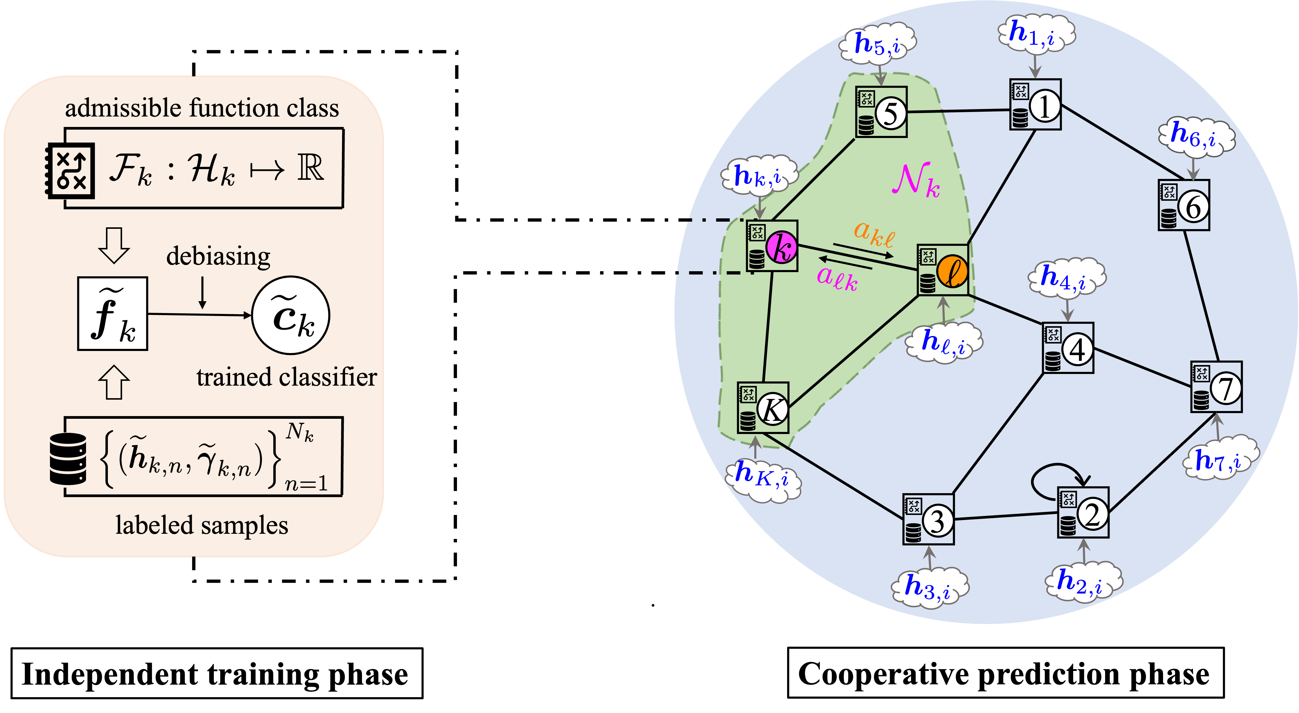
Figure 1: SML architecture. (Left panel): The independent training process where each agent $k$ finds an optimal model, namely function $\widetilde{\bm{f}}_{k}$, from an admissible function class $\mathcal{F}_{k}$, based on its training set and constructs the classifier $\widetilde{\bm{c}}_{k}$ involving a debiasing operation for the subsequent prediction phase. (Right panel): The cooperative classification process where each agent $k$ receives a sequence of streaming observations $\bm{h}_{k,i}$ and implements a social learning protocol to enhance the prediction performance. The neighboring set $\mathcal{N}_{k}$ of agent $k$ is marked by the area highlighted in green.

TABLE I: Main Symbols and Their Descriptions.

Notation	Description	Definition
$h$, $\gamma$	generic feature vector and the corresponding label	/
$\mathcal{K}$, $\Gamma$	set of agents and set of binary hypotheses	/
$(\widetilde{\bm{h}}_{k,n}$, $\widetilde{\bm{\gamma}}_{k,n})$	$n$-th training sample of agent $k$	/
$\mathcal{H}_{k}$, $\mathcal{F}_{k}$	feature space and function class of agent $k$	/
$c_{k}(h)$	logit of feature vector $h$ at agent $k$	(2)
$\widetilde{\bm{f}}_{k}$	optimal function for empirical risk of agent $k$	(5)
$\widetilde{\bm{c}}_{k}(h)$	decision statistic for feature vector $h$ of agent $k$	(7)
$A$, $\pi$	combination policy and its Perron eigenvector	(12), (13)
$\bm{h}_{k,i}$, $\bm{\gamma}_{0}$	observation of agent $k$ and the true state in statistical classification	/
$\bm{\lambda}_{k,i}$, $\bm{\gamma}_{k,i}$	agent $k$’s log-belief ratio at time $i$ and its decision	(14), (45)
$\widehat{\bm{\lambda}}_{k}$	asymptotic decision statistic	(18)
$\widetilde{\bm{\mu}}_{k}(f_{k})$, $\widetilde{\bm{\mu}}(f)$	individual empirical training mean and the network average quantity	(8), (23)
$\mu_{k}^{+}(f_{k})$, $\mu_{k}^{-}(f_{k})$	conditional means associated with $f_{k}$ under two hypotheses	(19)
$\mu^{+}(f)$, $\mu^{-}(f)$	network average quantities for the conditional means	(21)
$\widetilde{\bm{R}}_{k}(f_{k})$, $R_{k}(f_{k})$	empirical and expected risks associated with $f_{k}$	(6), (26)
$\mathsf{R}_{k}^{o}$, $\mathsf{R}^{o}$	individual target risk and the network average quantity	(25)
$\widetilde{\bm{R}}(f)$, $R(f)$	network average quantities for the empirical and expected risks	(30)
$\mathcal{R}(\mathcal{F}_{k}(h^{(k)}))$	empirical Rademacher complexity of agent $k$ for a sample set $h^{(k)}$	(32)
$\rho_{k}$, $\rho$	individual and network expected Rademacher complexities	(33), (34)
$\alpha$, $\beta$	network imbalance penalty and the bound of functions	(36), /
$\delta$	decision margin	(47)
$P_{c}$, $P_{c,\delta}$	probabilities of consistent training and $\delta$-margin consistent training	(24), (48)
$P_{e}$, $P_{k,i}^{e}$	probability of error and the instantaneous one for agent $k$ at time $i$	(40), (46)
$\mathcal{M}_{k,i}$, $\mathcal{M}_{s}$	events of misclassification	(51), (73)
$\mathcal{C}_{\delta}$	event of $\delta$-margin consistent training	(52)
$\bm{h}_{k,{\sf s}}$, $\bm{\gamma}_{\sf s}$	feature vector and its label in the single-sample classification task	/
$\bm{\lambda}_{{\sf s}}$, $\widehat{\bm{\gamma}}_{\sf s}$	decision statistic and predicted label in single-sample classification	(69), (70)
$\widetilde{\bm{c}}_{\sf s}(\bm{h}_{\sf s})$	prediction of the SML strategy as an ensemble classifier	(71)
$\mathdutchcal{E}(\mathsf{R}^{o},\delta)$	quantity related to the difficulty of the classification task	(102)

III The SML strategy

We consider a network of $K$ connected agents or classifiers indexed by $k\in\mathcal{K}\triangleq\{1,2,\dots,K\}$, trying to solve a binary classification task. The agents are heterogeneous in that their observations may follow different statistical models even when they are attributed to the same class. An example of this situation arises in multi-view learning [30], where each agent observes a different perspective of the same phenomenon and seeks to uncover the underlying state. In Fig. 1, we present a diagram of the SML architecture. We denote the set of binary hypotheses by $\Gamma=\{+1,-1\}$. In the independent training phase shown on the left, each agent $k$ has a set of $N_{k}$ labeled examples consisting of pairs $\{(\widetilde{\bm{h}}_{k,n},\widetilde{\bm{\gamma}}_{k,n})\}_{n=1}^{N_{k}}$, where $\widetilde{\bm{h}}_{k,n}$ is the $n$-th feature vector and $\widetilde{\bm{\gamma}}_{k,n}\in\Gamma$ is the corresponding label. The feature space of agent $k$ is denoted by $\mathcal{H}_{k}$. Recall that, in our notation, we use the $\sim$ symbol on top of variables associated with the training phase. The pair $(\widetilde{\bm{h}}_{k,n},\widetilde{\bm{\gamma}}_{k,n})$ is distributed according to

$$(\widetilde{\bm{h}}_{k,n},\widetilde{\bm{\gamma}}_{k,n})\sim\widetilde{p}_{k}(h,\gamma)=L_{k}(h|\gamma)\widetilde{p}_{k}(\gamma),$$ (1)

where $L_{k}(h|\gamma)$ is the unknown likelihood model and $\widetilde{p}_{k}(\gamma)$ is the class probability in the training set. Although unnecessary, we assume that the training set is balanced, i.e., $\widetilde{p}_{k}(\gamma)=\frac{1}{2}$. For the binary classification problem, the logit (i.e., log-ratio between posterior probabilities), defined as

$$c_{k}(h)\triangleq\log\frac{\widetilde{p}_{k}(+1|h)}{\widetilde{p}_{k}(-1|h)},$$ (2)

is an important decision statistic for labeling the observed feature vector $h$. For example, we know that the optimal Bayes classifier would assign $h$ to class $\gamma=+1$ if $c_{k}(h)$ is positive and to class $\gamma=-1$ otherwise. Under the uniform prior condition, the logit reduces to the log-likelihood ratio:

$$c_{k}(h){=}\log\frac{L_{k}(h|+1)}{L_{k}(h|-1)}.$$ (3)

Since the likelihood models $L_{k}(h|\gamma)$ are unknown, the logit function $c_{k}$ is not accessible and will need to be learned in the SML strategy, whose operation is described next following [9].

III-A Training phase

In the training phase, each agent employs a discriminative learning paradigm and generates an output for the classifier that approximates posterior probabilities for each class, denoted by $\widehat{p}_{k}(+1|h)$ and $\widehat{p}_{k}(-1|h)$. For example, each classifier could be implemented in the form of a logistic classifier or a neural network. The approximate logit statistic is then given by

$$\log\frac{\widehat{p}_{k}(+1|h)}{\widehat{p}_{k}(+1|h)}\triangleq f_{k}(h)$$ (4)

where the function $f_{k}$ belongs to some admissible class $\mathcal{F}_{k}:\mathcal{H}_{k}\mapsto\mathbb{R}$. The form of $f_{k}$ depends on the type of classifier implemented at the agent. By training the classifier, agents are able to optimize the parameters that determine the form of $f_{k}$. In order to find the best function $\widetilde{\bm{f}}_{k}$, we employ an empirical risk minimization formulation and minimize a suitable risk function based on the training samples:

$$\widetilde{\bm{f}}_{k}\triangleq\operatorname*{arg\min}_{f_{k}\in\mathcal{F}_{k}}\widetilde{\bm{R}}_{k}(f_{k}),$$ (5)

where $\widetilde{\bm{R}}_{k}(f_{k})$ is defined as

$$\widetilde{\bm{R}}_{k}(f_{k})\triangleq\frac{1}{N_{k}}\sum_{n=1}^{N_{k}}\phi\left({\widetilde{\bm{\gamma}}_{k,n}f_{k}(\widetilde{\bm{h}}_{k,n})}\right)$$ (6)

for some loss function $\phi$ that satisfies the following conditions.

Assumption 1 (Conditions on the loss function).

The loss function $\phi:\mathbb{R}\mapsto\mathbb{R}_{+}$ is convex, non-increasing and differentiable at $0$ with $\phi^{\prime}(0)<0$. Also, it is $L_{\phi}$-Lipschitz. ∎

This assumption guarantees the loss function $\phi$ to be classification-calibrated (see Theorem 2 in [31]), which implies that the function $\widetilde{\bm{f}}_{k}$ will be Bayes-risk optimal when there is an infinite number of training samples, i.e., $N_{k}\to\infty$ in (6). Put differently, $\widetilde{\bm{f}}_{k}(h)$ and $c_{k}(h)$ will have the same sign for any feature vector $h\in\mathcal{H}_{k}$. Due to this useful property, classification-calibrated loss functions are extensively utilized for classification tasks in the literature. In [9], the logistic loss $\phi_{\sf{log}}(x)=\log(1+e^{-x})$ is considered. It is clear that $\phi_{\sf{log}}$ satisfies all the conditions of Assumption 1 with $L_{\phi}=1$. In addition to the logistic loss, Assumption 1 covers many other widely-used loss functions, including the exponential loss $\phi(x)=e^{-x}$ used in AdaBoost and related boosting algorithms [25, 27], the hinge loss $\phi(x)=\max(0,1-x)$ used in support vector machines [32], and the truncated quadratic loss $\phi(x)=\{\max(0,1-x)\}^{2}$. All results of this paper are presented considering a generic loss function $\phi$ under Assumption 1.

In this paper, we consider classifiers that belong to the general class of bounded real-valued functions $\mathcal{F}_{k}$. The following assumption on the function $f_{k}$ is imposed.

Assumption 2 (Boundedness of functions).

There exists a constant $\beta>0$ such that $\forall h\in\mathcal{H}_{k}$, $\absolutevalue{f_{k}(h)}\leq\beta$ for each agent $k\in\mathcal{K}$ and each function $f_{k}\in\mathcal{F}_{k}$. ∎

After the training phase, the learned function $\widetilde{\bm{f}}_{k}$ in (5) at agent $k$ is utilized to generate a local decision statistic, denoted by $\widetilde{\bm{c}}_{k}(h)$, for the unseen feature vector $h\in\mathcal{H}_{k}$ as follows:

$$\widetilde{\bm{c}}_{k}(h)\triangleq\widetilde{\bm{f}}_{k}(h)-\widetilde{\bm{\mu}}_{k}(\widetilde{\bm{f}}_{k}),$$ (7)

where $\widetilde{\bm{\mu}}_{k}(\widetilde{\bm{f}}_{k})$ is the empirical training mean calculated by

$$\widetilde{\bm{\mu}}_{k}(f_{k})\triangleq\frac{1}{N_{k}}\sum_{n=1}^{N_{k}}f_{k}(\widetilde{\bm{h}}_{k,n}),\quad\forall f_{k}\in\mathcal{F}_{k}.$$ (8)

Discounting the empirical training mean is suggested in [9] as a debiasing operation to mitigate possible biased models resulting from the training process. In summary, the objective of the training phase is to use the training data $(\widetilde{\bm{h}}_{k,n},\widetilde{\bm{\gamma}}_{k,n})$ to arrive at the classifier models $\{\widetilde{\bm{c}}_{k}\}$; one for each agent.

III-B Prediction phase

In the prediction (testing) phase, the dispersed agents work jointly to solve a binary classification problem using their independently trained classifiers $\{\widetilde{\bm{c}}_{k}\}$ constructed from (7). The work [9] assumes an infinite number of streaming samples. Specifically, at each time $i$, each agent $k$ receives a new feature vector $\bm{h}_{k,i}\in\mathcal{H}_{k}$, so that each agent $k$ has access to a growing stream of feature vectors

$$\bm{h}_{k,1},\bm{h}_{k,2},\dots$$ (9)

which are identically independently distributed (i.i.d.) according to the unknown likelihood model $L_{k}(\cdot|\bm{\gamma}_{0})$, where $\bm{\gamma}_{0}\in\Gamma$ is the true state in force during the prediction phase. For any time $i$, the feature vectors $\{\bm{h}_{k,i}\}$ observed by all agents are assumed to be mutually independent conditioned on the truth $\bm{\gamma}_{0}$. We use the boldface font $\bm{\gamma}_{0}$ here to highlight that the true state is a random variable within the prediction phase, i.e., for each classification task. The class probability of $\bm{\gamma}_{0}$ is denoted by $P(\bm{\gamma}_{0})$. To solve this classification problem under infinite samples, a distributed learning rule inspired by the studies on social learning under knowledge of likelihood models [12, 13, 14, 15, 16, 17] is formulated in the SML strategy. For clarity, we next briefly describe the basic framework of social learning rules.

When the accurate likelihood models $L_{k}(h|\gamma)$ are available, different social learning rules have been proposed in the literature, all of which rely on iterative adaptation and combination steps. Let $\bm{\varphi}_{k,i}$ be the belief vector of agent $k$ at time $i$, which is a probability mass function over the set of hypotheses $\Gamma$. Each entry $\bm{\varphi}_{k,i}(\gamma)$ represents agent $k$’s confidence at time $i$ that $\gamma$ is the true state, i.e., that $\gamma=\bm{\gamma}_{0}$. In the adaptation step, the Bayes rule is employed to incorporate information about the new observation $\bm{h}_{k,i}$ into the agent’s intermediate belief $\bm{\psi}_{k,i}$:

$$\bm{\psi}_{k,i}(\gamma)=\frac{\bm{\varphi}_{k,i-1}(\gamma)L_{k}(\bm{h}_{k,i}|\gamma)}{\sum_{\gamma^{\prime}\in\Gamma}\bm{\varphi}_{k,i-1}(\gamma^{\prime})L_{k}(\bm{h}_{k,i}|\gamma^{\prime})},\quad\forall\gamma\in\Gamma.$$ (10)

On the other hand, in the combination step, each agent aggregates the information (i.e., intermediate beliefs) from its neighbors using a certain pooling protocol. One representative protocol, which is also considered in this work, is the geometric protocol described as:

$$\bm{\varphi}_{k,i}(\gamma)=\frac{\exp{\sum_{\ell\in\mathcal{N}_{k}}a_{\ell k}\log\bm{\psi}_{\ell,i}(\gamma)}}{\sum_{\gamma^{\prime}\in\Gamma}\exp{\sum_{\ell\in\mathcal{N}_{k}}a_{\ell k}\log\bm{\psi}_{\ell,i}(\gamma^{\prime})}}$$ (11)

for each $\gamma\in\Gamma$. The combination weight $a_{\ell k}$ that agent $k$ assigns to its neighbor $\ell$ satisfies:

$$\sum_{\ell=1}^{K}a_{\ell k}=1,\quad a_{\ell k}>0,\;\;\forall\ell\in\mathcal{N}_{k},$$ (12)

and $a_{\ell k}=0$ if $\ell\notin\mathcal{N}_{k}$, where $\mathcal{N}_{k}$ denotes the neighboring set of agent $k$ (see Fig. 1 for an illustration). We have the following assumption on the network topology.

Assumption 3 (Strongly-connected graph).

The underlying graph of the network is strongly-connected. That is, there exist paths with positive combination weights between any two distinct agents in both directions (these trajectories need not be the same), and at least one agent has a self-loop, i.e., $a_{mm}>0$ for some agent $m$ [33]. ∎

Under this assumption and from the Perron-Frobenius theorem [33, 3], we know that the combination matrix $A=[a_{\ell k}]$ is primitive and has a Perron eigenvector $\pi$ satisfying:

$$A\pi=\pi,\quad\sum_{k=1}^{K}\pi_{k}=1,\quad\pi_{k}>0,\quad\forall k\in\mathcal{K}.$$ (13)

Furthermore, the second largest-magnitude eigenvalue of $A$ is strictly smaller than 1. The social learning rule (10)–(11) can be written in a compact form by introducing the log-belief ratio between labels $+1$ and $-1$, denoted by:

$$\bm{\lambda}_{k,i}\triangleq\log\frac{\bm{\varphi}_{k,i}(+1)}{\bm{\varphi}_{k,i}(-1)}.$$ (14)

It is clear that $\bm{\lambda}_{k,i}$ represents the preference of agent $k$ for classification at time $i$: label $+1$ (or $-1$) will be selected if $\bm{\lambda}_{k,i}$ is positive (or negative). Combining (10) and (11), the log-belief ratio satisfies the following iteration:

$$\bm{\lambda}_{k,i}=\sum_{\ell=1}^{K}a_{\ell k}\big{(}\bm{\lambda}_{\ell,i-1}+c_{\ell}({\bm{h}}_{\ell,i})\big{)}$$ (15)

where $c_{\ell}({\bm{h}}_{\ell,i})$ is the log-likelihood ratio given by (3).

As we explained before, the log-likelihood ratio is unknown in the SML framework and must be learned from the training samples. By replacing $c_{\ell}({\bm{h}}_{\ell,i})$ with the learned decision statistic $\widetilde{\bm{c}}_{\ell}(\bm{h}_{\ell,i})$, the following social learning rule is employed in the prediction phase (where we continue to use the $\bm{\lambda}$ notation to avoid an explosion in symbols):

$$\bm{\lambda}_{k,i}=\sum_{\ell=1}^{K}a_{\ell k}\big{(}\bm{\lambda}_{\ell,i-1}+\widetilde{\bm{c}}_{\ell}({\bm{h}}_{\ell,i})\big{)}.$$ (16)

An important feature of the distributed learning rule (16) is that the information from the local observations is aggregated over both space (through $\ell$) and time (through $i$), which strengthens the decision-making capabilities of the agents.

IV Consistency of the SML strategy

The SML strategy is called consistent if asymptotic truth learning in the prediction phase is attained [9], namely, if the true state $\bm{\gamma}_{0}$ is learned by all agents when the number of observations (i.e., feature vectors $\{\bm{h}_{k,i}\}$) goes to infinity. To examine consistency, we first recall an important conclusion about the social learning rule (16) from [15, 9], namely that

$$\frac{1}{i}\bm{\lambda}_{k,i}\overset{\text{a.s.}}{\longrightarrow}\sum_{k=1}^{K}\pi_{k}\mathbb{E}_{\bm{\gamma}_{0}}\widetilde{\bm{c}}_{k}(\bm{h}_{k,i})$$ (17)

where “a.s.” means almost sure convergence and $\mathbb{E}_{\bm{\gamma}_{0}}$ denotes the expectation operator w.r.t. the unknown feature distribution $L_{k}(\cdot|\bm{\gamma}_{0})$. For each agent $k\in\mathcal{K}$, we therefore introduce the following asymptotic decision statistic $\widehat{\bm{\lambda}}_{k}$:

$$\widehat{\bm{\lambda}}_{k}\triangleq\sum_{k=1}^{K}\pi_{k}\mathbb{E}_{\bm{\gamma}_{0}}\widetilde{\bm{c}}_{k}(\bm{h}_{k,i}).$$ (18)

Then, the SML strategy is consistent if $\bm{\gamma}_{0}\widehat{\bm{\lambda}}_{k}>0$ is satisfied for all $k\in\mathcal{K}$. That is, $\widehat{\bm{\lambda}}_{k}>0$ if $\bm{\gamma}_{0}=+1$, and $\widehat{\bm{\lambda}}_{k}<0$ otherwise. To avoid confusion, it is worth noting that the trained models $\{\widetilde{\bm{f}}_{k}\}$ and classifiers $\{\widetilde{\bm{c}}_{k}\}$ are generated in the training phase, so they are random w.r.t. the training set. Given a particular training setup, we can “freeze” the randomness of the training set and work conditionally on the resulting realization of $\{\widetilde{f}_{k}\}$ and $\{\widetilde{c}_{k}\}$.

Let $\mu_{k}^{+}(f_{k})$ and $\mu_{k}^{-}(f_{k})$ denote the conditional means of a function $f_{k}\in\mathcal{F}_{k}$ under the two hypotheses:

$$\mu_{k}^{+}(f_{k})\triangleq\mathbb{E}_{+1}f_{k}(\bm{h}_{k,i})=\mathbb{E}_{\bm{h}_{k,i}\sim L_{k}(\cdot|+1)}f_{k}(\bm{h}_{k,i}),$$ (19)

$$\mu_{k}^{-}(f_{k})\triangleq\mathbb{E}_{-1}f_{k}(\bm{h}_{k,i})=\mathbb{E}_{\bm{h}_{k,i}\sim L_{k}(\cdot|-1)}f_{k}(\bm{h}_{k,i}).$$ (20)

The network averages of these conditional means are defined according to

$$\mu^{+}(f)\triangleq\sum_{k=1}^{K}\pi_{k}\mu_{k}^{+}(f_{k}),\quad\mu^{-}(f)\triangleq\sum_{k=1}^{K}\pi_{k}\mu_{k}^{-}(f_{k}),$$ (21)

where the argument $f$ represents the dependence of the network averages $\mu^{+}(\cdot)$ and $\mu^{-}(\cdot)$ on the collection of functions $\{f_{k}\}$, i.e., $\mu^{+}(f)=\mu^{+}(f_{1},\dots,f_{K})$. Similar notation will be used for other networked quantities in this paper. Based on the social learning rule (16) and its convergence property in (17), the following sufficient conditions for consistent learning within the SML paradigm, given a particular training setup, are established in [9]:

$$\mu^{+}(\widetilde{f})>\widetilde{\mu}({\widetilde{f}})\quad\text{and}\quad\mu^{-}(\widetilde{f})<\widetilde{\mu}(\widetilde{f})$$ (22)

where

$$\widetilde{\mu}(\widetilde{f})\triangleq\sum_{k=1}^{K}\pi_{k}\widetilde{\mu}_{k}(\widetilde{f}_{k})$$ (23)

is the network average of the empirical training means specified in (8). Since the description (22) is given conditionally on a set of trained models $\{\widetilde{f}_{k}\}$, the conditions in (22) depend on the randomness stemming from the training phase. For this reason, these conditions will be referred to as the conditions for consistent training, namely, for the training set to produce a consistent classifier for the prediction phase at the end of the training phase. The probability of consistent training, denoted by $P_{c}$, is defined as follows:

$$P_{c}\triangleq\mathbb{P}\left(\mu^{+}(\widetilde{\bm{f}})>\widetilde{\bm{\mu}}({\widetilde{\bm{f}}}),\mu^{-}(\widetilde{\bm{f}})<\widetilde{\bm{\mu}}(\widetilde{\bm{f}})\right)$$ (24)

where the boldface fonts are used to highlight the randomness in the training phase. Using similar techniques as the ones used in [9], we will show in Lemma 1 that $P_{c}$ is lower bounded by a constant related to the number of training samples $N_{k}$, the Rademarcher complexity of function class $\mathcal{F}_{k}$, the Perron eigenvector $\pi$ of combination matrix $A$, and the properties of loss function $\phi$. For that purpose, we need to introduce some useful notation as follows. First, we define the target risk at every agent $k$ and the weighted network average of target risks as follows:

$$\mathsf{R}_{k}^{o}\triangleq\inf_{f_{k}\in\mathcal{F}_{k}}R_{k}(f_{k}),\quad\mathsf{R}^{o}\triangleq\sum_{k=1}^{K}\pi_{k}\mathsf{R}_{k}^{o},$$ (25)

where $R_{k}(f_{k})$ is the expected risk associated with $f_{k}$:

$$R_{k}(f_{k})\triangleq\mathbb{E}_{\widetilde{h}_{k},\widetilde{\gamma}_{k}}\phi\left(\widetilde{\bm{\gamma}}_{k,n}f_{k}(\widetilde{\bm{h}}_{k,n})\right).$$ (26)

Here, $\mathbb{E}_{\widetilde{h}_{k},\widetilde{\gamma}_{k}}$ denotes the expectation operator w.r.t. the unknown distribution $\widetilde{p}_{k}(h,\gamma)$ of the training pair $(\widetilde{\bm{h}}_{k,n},\widetilde{\bm{\gamma}}_{k,n})$ described in (1). We will assume that the target risk $\mathsf{R}^{o}$ is strictly smaller than $\phi(0)$, which in view of (26), is the risk corresponding to the uninformative classifier $f_{k}=0$. Formally, we assume

$$\mathsf{R}^{o}<\phi(0).$$ (27)

This condition eliminates the trivial case where $f_{k}=0$ is the optimal classifier for all $k\in\mathcal{K}$. To understand this condition, we recall the definition of $f_{k}$ from (4). Suppose that $f_{k}(h)=0$ for all $h\in\mathcal{H}_{k}$, then it will hold that

$$\widehat{p}_{k}(\gamma|h)=\frac{1}{2},\text{ for any }h\in\mathcal{H}_{k}\text{ and }\gamma\in\Gamma.$$ (28)

Consequently, agent $k$ will make an uninformed decision that randomly assigns the labels $+1$ and $-1$ with equal probability to all feature vectors. In other words, this agent fails to learn any discriminative information for the two classes based on its training set and the admissible function class. In comparison, according to definition (25), condition (27) implies that there exists some agent $k$ such that

$$\mathsf{R}^{o}_{k}<\phi(0).$$ (29)

That is, the uninformative classifier $f_{k}=0$ is not optimal for agent $k$. Put differently, condition (27) ensures that there is at least one agent that is capable of making a better decision than random guessing.

In a manner similar to the target risk, the weighted network averages for the empirical and expected risks (6) and (26) are defined as follows:

$$\widetilde{\bm{R}}(f)\triangleq\sum_{k=1}^{K}\pi_{k}\widetilde{\bm{R}}_{k}(f_{k}),\quad R(f)\triangleq\sum_{k=1}^{K}\pi_{k}R_{k}(f_{k}).$$ (30)

Next, we introduce some notation related to the Rademacher complexity of function classes $\{\mathcal{F}_{k}\}$ [3, 34]. Let

$$h^{(k)}\triangleq\big{\{}h_{k,1},\dots,h_{k,N_{k}}\big{\}}$$ (31)

be a fixed sample set of size $N_{k}$ for agent $k$. The individual empirical Rademacher complexity of agent $k$ for the sample set $h^{(k)}$ is defined as

$$\mathcal{R}(\mathcal{F}_{k}(h^{(k)}))\triangleq\mathbb{E}_{\bm{r}}\sup_{f_{k}\in\mathcal{F}_{k}}\absolutevalue{\frac{1}{N_{k}}\sum_{n=1}^{N_{k}}\bm{r}_{n}f_{k}(h_{k,n})}$$ (32)

where $\bm{r}=(\bm{r}_{1},\dots,\bm{r}_{N_{k}})$ is a sequence of i.i.d. Rademacher random variables. Namely, $\mathbb{P}(\bm{r}_{n}=+1)=\mathbb{P}(\bm{r}_{n}=-1)=1/2$. The quantity $\mathcal{R}(\mathcal{F}_{k}(h^{(k)}))$ measures on average how well the function class $\mathcal{F}_{k}$ correlates with random noise on $h^{(k)}$, and thus describes the richness of $\mathcal{F}_{k}$. The individual expected Rademacher complexity is defined as

$$\rho_{k}\triangleq\mathbb{E}_{{\bm{h}}^{(k)}}\mathcal{R}(\mathcal{F}_{k}(\bm{h}^{(k)})),$$ (33)

which is the expectation of $\mathcal{R}(\mathcal{F}_{k}(h^{(k)}))$ over all sample sets of size $N_{k}$ drawn according to (1). We also define the expected network Rademacher complexity according to

$$\rho\triangleq\sum_{k=1}^{K}\pi_{k}\rho_{k}.$$ (34)

With the above definitions, we can establish a lower bound on the probability of consistent training in (24) as follows.

Lemma 1 (Probability of consistent training).

Assume $\rho<\mathdutchcal{E}(\mathsf{R}^{o},0)$, where $\mathdutchcal{E}(\mathsf{R}^{o},0)$ is defined by (107) in Appendix A. Under Assumptions 1–3 and condition (27), the probability of consistent training $P_{c}$ in (24) is lower bounded by

$$P_{c}\geq 1-2\exp\left\{-\frac{8N_{\max}}{\alpha^{2}\beta^{2}}\Big{(}\mathdutchcal{E}(\mathsf{R}^{o},0)-\rho\Big{)}^{2}\right\},$$ (35)

where

$$N_{\max}\triangleq\max_{k}N_{k},\quad\alpha\triangleq\sum_{k=1}^{K}\pi_{k}\frac{N_{\max}}{N_{k}}.$$ (36)

Proof.

See Appendix A. ∎

The quantity $\alpha$ is called the network imbalance penalty, which quantifies how unequal the numbers of training samples are across different agents. Lemma 1 is an extension of the SML consistency result obtained exclusively for the logistic loss $\phi_{\sf log}$ in [9], where the expression of $\mathdutchcal{E}(\mathsf{R}^{o},0)$ was computed explicitly. Deriving the closed form of $\mathdutchcal{E}(\mathsf{R}^{o},0)$ for a general loss function $\phi$ that satisfies Assumption 1 is not a trivial task, since it requires us to solve the generic equation (100) provided in Appendix A.

The most important implication from Lemma 1 is that the probability of consistent training is bounded in an exponential manner if the network Rademacher complexity $\rho$ is smaller than the function $\mathdutchcal{E}(\mathsf{R}^{o},0)$. According to (105) in Appendix A, the following relation holds for $\mathdutchcal{E}(\mathsf{R}^{o},0)$:

$$\mathdutchcal{E}(\mathsf{R}^{o},0)\triangleq\frac{d_{0}^{\star}}{4}=\frac{\phi(d_{0}^{\star})-\mathsf{R}^{o}}{8L_{\phi}}$$ (37)

where $d_{0}^{\star}$ is the critical value for determining $\mathdutchcal{E}(\mathsf{R}^{o},0)$ and is derived by solving (100). Using a first-order approximation for the function $\phi$ around $0$, we have

$$\phi(d_{0}^{\star})\approx\phi(0)+\phi^{\prime}(0)d_{0}^{\star}$$ (38)

and

$$d_{0}^{\star}\approx\frac{\phi(0)-\mathsf{R}^{o}}{2L_{\phi}-\phi^{\prime}(0)}.$$ (39)

As already discussed for (27), the risk $\phi(0)$ corresponds to the uninformative classifier, i.e., to the case of classification by randomly guessing. Therefore, the quantity $\phi(0)-\mathsf{R}^{o}$ captures the difficulty of the binary classification task for the network. The closer the target risk $\mathsf{R}^{o}$ is to the uninformative risk $\phi(0)$, the smaller the value of $\mathdutchcal{E}(\mathsf{R}^{o},0)$ and consequently, the more restricted (due to the assumption of $\rho<\mathdutchcal{E}(\mathsf{R}^{o},0)$) the complexity of the classifier structure will be. Therefore, Eq. (35) reveals a remarkable interplay between the inherent difficulty of the classification problem (quantified by $\mathdutchcal{E}(\mathsf{R}^{o},0)$) and the complexity of the classifier structure (quantified by $\rho$).

The probability of error achieved by the SML strategy is defined as the probability of inconsistent learning:

$$P_{e}\triangleq\mathbb{P}\Big{(}\bm{\gamma}_{0}\widehat{\bm{\lambda}}_{k}\leq 0\Big{)}$$ (40)

where the randomness stems from both the training phase (i.e., the training set) and the prediction phase (i.e., the true label $\bm{\gamma}_{0}$). We next show that an upper bound for $P_{e}$ can be obtained from the probability of consistent training $P_{c}$. Combining the convergence result (17) with the definitions (7), (21), and (23), we have

$$\widehat{\bm{\lambda}}_{k}{=}\begin{cases}\mu^{+}(\widetilde{\bm{f}})-\widetilde{\bm{\mu}}(\widetilde{\bm{f}}),&\bm{\gamma}_{0}=+1,\\ \mu^{-}(\widetilde{\bm{f}})-\widetilde{\bm{\mu}}(\widetilde{\bm{f}}),&\bm{\gamma}_{0}=-1.\end{cases}$$ (41)

This yields

$$P_{e}\overset{\eqref{eq: P_e definition}}{=} \;\mathbb{P}(\bm{\gamma}_{0}=+1)\mathbb{P}\Big{(}\widehat{\bm{\lambda}}_{k}\leq 0|\bm{\gamma}_{0}=+1\Big{)}$$

$$+\mathbb{P}(\bm{\gamma}_{0}=-1)\mathbb{P}\Big{(}\widehat{\bm{\lambda}}_{k}\geq 0|\bm{\gamma}_{0}=-1\Big{)}$$

$$\overset{\eqref{eq: convergence under different hypotheses}}{=} \;P(+1)\mathbb{P}\Big{(}\mu^{+}(\widetilde{\bm{f}})-\widetilde{\bm{\mu}}(\widetilde{\bm{f}})\leq 0\Big{)}$$

$$+P(-1)\mathbb{P}\Big{(}\mu^{-}(\widetilde{\bm{f}})-\widetilde{\bm{\mu}}(\widetilde{\bm{f}})\geq 0\Big{)}$$

$${\leq} \;P(+1)(1-P_{c})+P(-1)(1-P_{c})$$

$$= \;1-P_{c}$$ (42)

where the inequality is due to the definition (24) of $P_{c}$, which guarantees:

$$1-P_{c}=\mathbb{P}\Big{(}\Big{\{}\mu^{+}(\widetilde{\bm{f}})-\widetilde{\bm{\mu}}(\widetilde{\bm{f}})\leq 0\Big{\}}\cup\Big{\{}\mu^{-}(\widetilde{\bm{f}})-\widetilde{\bm{\mu}}(\widetilde{\bm{f}})\geq 0\Big{\}}\Big{)}.$$ (43)

Therefore, when the number of observations for inference is large enough in the prediction phase, the probability of error attained by the SML strategy is upper bounded by $1-P_{c}$, which can be further refined using Lemma 1.

V Non-asymptotic performance for statistical classification tasks

In this section, we analyze the probability of error for the statistical classification task with a finite number of observations. In this setting, the agents try to identify the true label $\bm{\gamma}_{0}$ given a finite sequence of streaming feature vectors:

$$\bm{h}_{k,1},\bm{h}_{k,2},\dots,\bm{h}_{k,S}$$ (44)

where $S$ is the size of the stream of unlabeled samples in the prediction phase. It is notable that when $S$ tends to infinity, we will recover the classical social learning problem [9], whose probability of error can be upper bounded by $1-P_{c}$ as shown by (42). Since $S$ is finite, a non-asymptotic performance analysis for the distributed learning rule (16) is needed. To this end, we characterize the instantaneous probability of error for each agent $k$. Let $\bm{\gamma}_{k,i}$ denote agent $k$’s decision at time $i$. It is obvious that $\bm{\gamma}_{k,i}$ depends on the observations received by the network up to time $i$. Without loss of generality, we assume a uniform initial belief condition for the distributed learning rule (16), i.e., $\bm{\lambda}_{k,0}=0,\forall k\in\mathcal{K}$.

At each time $i$, the agents make a decision according to the sign of their log-belief ratios, i.e.,

$$\bm{\gamma}_{k,i}\triangleq\operatorname*{sign}(\bm{\lambda}_{k,i}).$$ (45)

Hence, a misclassification occurs at agent $k$ if $\bm{\lambda}_{k,i}$ and $\bm{\gamma}_{0}$ have different signs. Let $P_{k,i}^{e}$ denote the instantaneous probability of error associated with agent $k$ at time $i$:

$$P_{k,i}^{e}\triangleq\mathbb{P}\big{(}\bm{\gamma}_{0}\bm{\lambda}_{k,i}\leq 0\big{)}.$$ (46)

Before analyzing (46), we introduce another condition related to the performance of the training phase, which we refer to as the $\delta$-margin consistent training condition. This condition is similar to the consistent training condition in (22) established for the infinite-sample classification problem, which connects the performance of the training phase (i.e., $P_{c}$) with that of the prediction phase (i.e., $P_{e}$) through (42). We will show that the $\delta$-margin consistent training condition plays a key role in our subsequent non-asymptotic performance analysis. Formally, the $\delta$-margin consistent training condition, conditionally on a given set of trained models $\{\widetilde{f}_{k}\}$, is expressed by:

$$\mu^{+}(\widetilde{f})>\widetilde{\mu}({\widetilde{f}})+\delta\quad\text{and}\quad\mu^{-}(\widetilde{f})<\widetilde{\mu}(\widetilde{f})-\delta$$ (47)

where $\delta\geq 0$ is a non-negative constant. In view of (41), the parameter $\delta$ describes the distance between the asymptotic decision statistic $\widehat{\bm{\lambda}}_{k}$ and the decision boundary $0$, which we will refer to as the decision margin. To avoid confusion, we note that $\delta$ is a design parameter for the $\delta$-margin consistent training condition. However, for each specified learning setup, we can evaluate the value of $\delta$ that is actually achieved in the SML strategy by calculating the value of associated variables $\mu^{+}(\widetilde{f})$, $\mu^{-}(\widetilde{f})$, and $\widetilde{\mu}(\widetilde{f})$.

It is clear that for any positive $\delta>0$, the $\delta$-margin consistent training condition (47) is stronger than the consistent training condition given by (22). Let $P_{c,\delta}$ denote the probability of $\delta$-margin consistent training:

$$P_{c,\delta}\triangleq\mathbb{P}\left(\mu^{+}(\widetilde{\bm{f}})>\widetilde{\bm{\mu}}({\widetilde{\bm{f}}})+\delta,\mu^{-}(\widetilde{\bm{f}})<\widetilde{\bm{\mu}}(\widetilde{\bm{f}})-\delta\right).$$ (48)

Here, we use boldface fonts to emphasize the fact that condition (47) depends on the randomness coming from the training phase. Notice that $P_{c,\delta}\leq P_{c}$ and $P_{c,0}=P_{c}$. A lower bound on $P_{c,\delta}$ is obtained as follows.

Lemma 2 (Probability of $\delta$-margin consistent training).

Assume that $0\leq\delta<\delta_{\max}$ and $\rho<\mathdutchcal{E}(\mathsf{R}^{o},\delta)$, where the definitions of $\delta_{\max}$ and $\mathdutchcal{E}(\mathsf{R}^{o},\delta)$ are respectively given by (106) and (105) in Appendix A. Then, we have the following bound for the probability of $\delta$-margin consistent training:

$$P_{c,\delta}\geq 1-2\exp\left\{-\frac{8N_{\max}}{\alpha^{2}\beta^{2}}\Big{(}\mathdutchcal{E}({\mathsf{R}^{o}},\delta)-\rho\Big{)}^{2}\right\}.$$ (49)

Proof.

See Appendix A. ∎

Comparing Lemmas 1 and 2, we see that the lower bounds on $P_{c}$ and $P_{c,\delta}$ differ only in the term $\mathdutchcal{E}({\mathsf{R}^{o}},\delta)$. By choosing $\delta=0$, we recover (35) from (49). According to (108) in Appendix A, we have:

$$\mathdutchcal{E}({\mathsf{R}^{o}},\delta)=\mathdutchcal{E}({\mathsf{R}^{o}},0)+\frac{\phi(d_{\delta}^{\star})-\phi(d_{0}^{\star})}{8L_{\phi}}$$ (50)

where $d_{\delta}^{\star}$ is the solution to equation (100) given in Appendix A. Furthermore, since $d_{\delta}^{\star}$ increases with $\delta$ as proved in Appendix A and $\phi$ is a non-increasing loss function under Assumption 1, the value of $\mathdutchcal{E}({\mathsf{R}^{o}},\delta)$ is also non-increasing with $\delta$. Accordingly, the lower bound on $P_{c,\delta}$ is not increased when a larger decision margin $\delta$ is obtained. Similar to (35), Eq. (49) demonstrates a remarkable interplay between the difficulty of classification problems and the complexity of classifier structures when a certain margin condition is imposed.

Let $\mathcal{M}_{k,i}$ denote the event of misclassification by agent $k$ at time $i$ and let $\mathcal{C}_{\delta}$ denote the event of $\delta$-margin consistent training:

$$\mathcal{M}_{k,i} \triangleq\big{\{}\bm{\gamma}_{0}\bm{\lambda}_{k,i}\leq 0\big{\}},$$ (51)

$$\mathcal{C}_{\delta} \triangleq\left\{{\mu^{+}}(\bm{\widetilde{\bm{f}}})-\bm{\widetilde{\bm{\mu}}}(\bm{\widetilde{\bm{f}}})>\delta,{\mu^{-}}(\bm{\widetilde{\bm{f}}})-\bm{\widetilde{\bm{\mu}}}(\bm{\widetilde{\bm{f}}})<-\delta\right\}.$$ (52)

According to the law of total probability, the following inequality holds for the instantaneous probability of error:

$$P_{k,i}^{e}\overset{\eqref{eq: instantaneous probability of error}}{=}\mathbb{P}(\mathcal{M}_{k,i}) =\mathbb{P}(\mathcal{M}_{k,i}\cap\mathcal{C}_{\delta})+\mathbb{P}(\mathcal{M}_{k,i}\cap\overline{\mathcal{C}_{\delta}})$$

$$=\mathbb{P}(\mathcal{C}_{\delta})\mathbb{P}\left(\mathcal{M}_{k,i}|\mathcal{C}_{\delta}\right)+\mathbb{P}(\overline{\mathcal{C}_{\delta}})\mathbb{P}\left(\mathcal{M}_{k,i}|\overline{\mathcal{C}_{\delta}}\right)$$

$$\leq\mathbb{P}\left(\mathcal{M}_{k,i}|\mathcal{C}_{\delta}\right)+\mathbb{P}(\overline{\mathcal{C}_{\delta}}).$$ (53)

Now since $\mathbb{P}(\overline{\mathcal{C}_{\delta}})=1-P_{c,\delta}$, which can be upper bounded by using Lemma 2, we can derive an upper bound on $P_{k,i}^{e}$ by characterizing the conditional probability $\mathbb{P}(\mathcal{M}_{k,i}|\mathcal{C}_{\delta})$. This is established in the following theorem.

Theorem 1 (Statistical classification error).

Let $\sigma$ denote the second largest-magnitude eigenvalue of combination matrix $A$ (which we know to be strictly less than one). Suppose that agents follow the social learning protocol (16), then under the $\delta$-margin consistent training condition (47), we have

$$\mathbb{P}(\mathcal{M}_{k,i}|\mathcal{C}_{\delta})\leq\exp\left\{-\frac{\left(\delta i-\kappa\right)^{2}}{2\beta^{2}i}\right\}$$ (54)

for all $i\geq\frac{\kappa}{\delta}$, where

$$\kappa\triangleq\frac{8\beta\log K}{1-\sigma}.$$ (55)

Hence, suppose the same assumptions as those in Lemma 2. Then, for any sequence of observations of size $S\geq\frac{\kappa}{\delta}$, the probability of classification error, denoted by $P_{k,S}^{e}$, is upper bounded by

$$P_{k,S}^{e}\leq \;2\exp\left\{-\frac{8N_{\max}}{\alpha^{2}\beta^{2}}\Big{(}\mathdutchcal{E}({\mathsf{R}^{o}},\delta)-\rho\Big{)}^{2}\right\}$$

$$+\exp\left\{-\frac{\left(\delta S-\kappa\right)^{2}}{2\beta^{2}S}\right\}.$$ (56)

Proof.

See Appendix B. ∎

We analyze next how we can relate the bound on the consistent training from Lemma 1 (for the infinite-sample case) to the result of Theorem 1 (for the finite-sample case). As the number of observations $S$ grows, the second term in (56) vanishes and $P_{k,S}^{e}$ approaches the first term, which is upper bounded by $1-P_{c,\delta}$. Since $P_{c,\delta}\leq P_{c}$, then in view of (42), $1-P_{c,\delta}$ is also an upper bound on the probability of error for the social learning problem (i.e., infinite-sample case). By letting $\delta\to 0$, we recover the upper bound $1-P_{c}$ established in (42). Furthermore, according to (56), it is expected that the decay rate of $P_{k,S}^{e}$ w.r.t. $S$ will be faster when a larger decision margin $\delta$ is achieved in the training phase.

Equation (54) provides a good estimate for the sample complexity in the prediction phase when the $\delta$-margin consistent training condition is achieved in the training phase. This is summarized in following Corollary 1, whose proof can be found in Appendix B.

Corollary 1 (Sample complexity).

Let $0<\epsilon<1$ be a prescribed error level, then one gets

$$\mathbb{P}\left[\mathcal{M}_{k,i}|\mathcal{C}_{\delta}\right]\leq\epsilon$$ (57)

after collecting more than $N_{\epsilon}$ feature vectors, where

$$N_{\epsilon}\triangleq\frac{\beta\sqrt{\beta^{2}(\log\epsilon)^{2}-2\kappa\delta\log\epsilon}-\beta^{2}\log\epsilon+\kappa\delta}{\delta^{2}}.$$ (58)

Theorem 1 demonstrates the effect of different parameters on the probability of error for the statistical classification task. In the following, we explain the roles of the network topology and the decision margin in more detail.

1) Role of the network: From (56), the classification error is related to two parameters pertaining to the combination policy $A$: the second largest-magnitude eigenvalue $\sigma$ and the Perron eigenvector $\pi$.

$\bullet$ Parameter $\sigma$: It is known that $\sigma$ describes the mixing rate of a Markov chain whose transition probability is given by matrix $A$ [3]. A smaller $\sigma$ indicates a faster mixing rate, which is beneficial for diffusion of information over the network [35]. The quantity $1-\sigma$ is also known as the spectral gap of the network. The spectral gap of different networks and its impact on the social learning performance is analyzed in [12]. Within the cooperative prediction phase where the information from all agents (i.e., intermediate belief vectors $\bm{\psi}_{k,i}$) diffuses across the network, a similar effect of $\sigma$ on $P_{k,S}^{e}$ is observed: the smaller the value of $\sigma$ is, the better upper bound we obtain in (56).

$\bullet$ Parameter $\pi$: The entries of the Perron eigenvector $\pi$ represent the centrality of each agent in determining the pertinent network parameters, such as $\rho$, $\alpha$, and $\mathsf{R}^{o}$ in Theorem 1. In view of the definitions of $\mu^{+}(f)$, $\mu^{-}(f)$, and $\widetilde{{\mu}}(f)$ in (21) and (23), these Perron entries also play an important role in the decision margin $\delta$ achieved by the training phase. Let us define the local decision margin attained by agent $k$ in the non-cooperative scenario as the quantity $\delta_{k}$ that satisfies:

$$\mu_{k}^{+}(\widetilde{\bm{f}}_{k})-\widetilde{\bm{\mu}}_{k}(\widetilde{\bm{f}}_{k})>\delta_{k},\quad\mu_{k}^{-}(\widetilde{\bm{f}}_{k})-\widetilde{\bm{\mu}}_{k}(\widetilde{\bm{f}}_{k})<-\delta_{k}.$$ (59)

An agent $k$ is considered to be more informative than another agent if its local decision margin $\delta_{k}$ is larger. Indeed, from the definitions of the $\delta$-margin consistent training condition (47) and the asymptotic decision statistic $\widehat{\bm{\lambda}}_{k}$ (41), it is seen that the decision margin $\delta$ achieved by the SML strategy is a weighted quantity of the local decision margins attained by each agent:

$$\delta=\sum_{k=1}^{K}\pi_{k}\delta_{k}.$$ (60)

Therefore, a larger decision margin associated with the SML strategy can be obtained if a higher centrality is placed on the more informative agents, namely, the agents with a better trained classifier. Compared to the social learning problem with accurate likelihood models, the informativeness of agents within the SML framework depends not only on the statistical properties of their local observations, but also on their ability (associated with $N_{k}$ and $\mathcal{F}_{k}$) to learn a good classifier in the training phase.

2) Role of the decision margin: The decision margin $\delta$ plays a similar role to that of the minimum weighted Kullback–Leibler (KL) divergence in the social learning problem when the likelihood models are known accurately [15, 13, 14, 12, 16, 17]. Let $\Delta$ denote the minimum weighted KL divergence calculated under the accurate likelihood models, and $\widetilde{\Delta}$ denote its approximated value that is learned from the training phase of the SML strategy. For the binary classification case, $\Delta$ is given by:

$$\Delta\triangleq\min\left\{\Delta^{+},\Delta^{-}\right\}$$ (61)

where

$$\Delta^{+}\triangleq\sum_{k=1}^{K}\pi_{k}D_{\textnormal{KL}}\left(L_{k}(\cdot|+1)\|L_{k}(\cdot|-1)\right),$$ (62)

$$\Delta^{-}\triangleq\sum_{k=1}^{K}\pi_{k}D_{\textnormal{KL}}\left(L_{k}(\cdot|-1)\|L_{k}(\cdot|+1)\right),$$ (63)

with $D_{\textnormal{KL}}(p\|q)$ denoting the KL divergence between two distributions $p$ and $q$[36]. For the geometric learning rule (16), it is shown in [12, 13, 14, 15, 16, 17] that the quantities $\Delta^{+}$ and $\Delta^{-}$ describe the difficulty of truth learning when the underlying state $\bm{\gamma}_{0}$ is $+1$ and $-1$, respectively. Hence, $\Delta$ captures the difficulty of distinguishing the two hypotheses by means of the social learning rule (16). To understand the connection between $\delta$ and $\Delta$, note that in the training phase, agents try to approximate the logit $c_{k}(h)$ given by (2) (or the log-likelihood ratio given by (3)) with $\widetilde{\bm{c}}_{k}(h)$ defined in (7). Therefore, the difficulty of learning with the trained classifiers $\widetilde{\bm{c}}_{k}$ depends on the following two quantities:

$$\widetilde{\Delta}^{+} =\sum_{k=1}^{K}\pi_{k}\mathbb{E}_{+1}\widetilde{\bm{c}}_{k}(h)=\mu^{+}(\widetilde{\bm{f}})-\widetilde{\bm{\mu}}(\widetilde{\bm{f}}),$$ (64)

$$\widetilde{\Delta}^{-} =-\sum_{k=1}^{K}\pi_{k}\mathbb{E}_{-1}\widetilde{\bm{c}}_{k}(h)=-\mu^{-}(\widetilde{\bm{f}})+\widetilde{\bm{\mu}}(\widetilde{\bm{f}}).$$ (65)

Hence, $\mu^{+}(\widetilde{\bm{f}})-\widetilde{\bm{\mu}}(\widetilde{\bm{f}})$ (or $\mu^{-}(\widetilde{\bm{f}})-\widetilde{\bm{\mu}}(\widetilde{\bm{f}})$) represents the difficulty of learning the true label $+1$ (or $-1$) using the trained classifiers $\widetilde{\bm{c}}_{k}$. By definition of the $\delta$-margin consistent training condition (47), we have

$$\widetilde{\Delta}\triangleq\min\left\{\widetilde{\Delta}^{+},\widetilde{\Delta}^{-}\right\}>\delta.$$ (66)

Therefore, for the given statistical classification task, a larger decision margin $\delta$ implies that the network, as a collection of dispersed agents, has obtained a better set of local classifiers in the training phase. This is consistent with (58), where an increasing $\delta$ is beneficial for faster truth learning.

VI Single-sample classification

For the single-sample classification problem, each observation received by the agents is taken as a testing sample to be labeled. This setting is the classical setup of classification tasks considered in the ML literature, which addresses the problem in a centralized manner by using a fusion center to assemble the local classifiers. While a centralized solution is applicable in many scenarios, the distributed decision-making architecture provides more flexibility and additional privacy guarantees. We explain next how to solve the single-sample classification task in a decentralized manner within the SML framework and examine the corresponding probability of error.

In this case, we will assume that the communication time is not a constraint for distributed learning, and study the classification error when the agents have enough time to make a collective decision before the arrival of the next testing sample. To avoid ambiguity, we use the variable $t$ to denote the number of communication rounds during the classification process. Specifically, once agent $k$ receives a new testing sample $\bm{h}_{k,{\sf s}}$ whose true label is $\bm{\gamma}_{\sf s}$, it first calculates the local decision statistic $\bm{\lambda}_{k,1}$ using the learned classifier $\widetilde{\bm{c}}_{k}$ from the training phase:

$$\bm{\lambda}_{k,1}\triangleq\widetilde{\bm{c}}_{k}(\bm{h}_{k,{\sf s}}).$$ (67)

Then, each agent communicates locally with its neighbors and updates its log-belief ratio as:

$$\bm{\lambda}_{k,t}=\sum_{\ell=1}^{K}a_{\ell k}\bm{\lambda}_{\ell,t-1}.$$ (68)

This is equivalent to performing the social learning rule (16) by taking $\widetilde{\bm{c}}_{\ell}(\bm{h}_{\ell,i})=0$ for any agent $\ell$ and for all $i>1$, since each agent receives only one unlabeled sample in this case. Under the strongly-connected assumption (Assumption 3), it is known [37, 3] that all agents finally agree on a common decision statistic $\bm{\lambda}_{{\sf s}}$ after sufficient communication rounds. That is,

$$\bm{\lambda}_{{\sf s}}\triangleq\lim\limits_{t\to\infty}\bm{\lambda}_{k,t}\overset{\text{a.s.}}{=}\sum_{k=1}^{K}\pi_{k}\widetilde{\bm{c}}_{k}(\bm{h}_{k,{\sf s}}).$$ (69)

It is worth mentioning that conditional on the training phase, $\bm{\lambda}_{{\sf s}}$ is a random variable w.r.t. the testing sample $\bm{h}_{k,{\sf s}}$. However, once the testing sample $\bm{h}_{k,{\sf s}}$ is given, $\bm{\lambda}_{{\sf s}}$ becomes a deterministic value. The classification decision $\widehat{\bm{\gamma}}_{\sf s}$ for the testing sample $\bm{h}_{k,{\sf s}}$ is given by the sign of $\bm{\lambda}_{{\sf s}}$, i.e.,

$$\widehat{\bm{\gamma}}_{\sf s}\triangleq\operatorname*{sign}(\bm{\lambda}_{{\sf s}}).$$ (70)

Obviously, the Perron eigenvector $\pi$ of the combination policy $A$ plays an important role in the classification performance of the SML strategy. In view of (69), the distributed learning rule (68) functions as a centralized ensemble classifier $\widetilde{\bm{c}}_{\sf s}$ denoted by:

$$\widetilde{\bm{c}}_{\sf s}(\bm{h}_{\sf s})\triangleq\sum_{k=1}^{K}\pi_{k}\widetilde{\bm{c}}_{k}(\bm{h}_{k,{\sf s}})$$ (71)

where

$$\bm{h}_{\sf s}\triangleq(\bm{h}_{1,{\sf s}},\dots,\bm{h}_{K,{\sf s}})$$ (72)

is the collection of local testing samples received by the $K$ agents. The ensemble classifier (71) resembles a $\pi$-weighted soft decision combination strategy for the multiple classifiers system involving an independent training phase. As reviewed in Section II, in contrast to hard decision combination strategies such as boosting [25] and majority voting [26], the theoretical performance analysis for the soft decision combination strategy is harder.

In the following, we show that by leveraging the $\delta$-margin consistent training condition (47) and the corresponding result in Lemma 2, an upper bound on the probability of error for the ensemble classifier (71) can be established. Let $\mathcal{M}_{s}$ denote the event of misclassification for the single-sample classification task:

$$\mathcal{M}_{s}\triangleq\big{\{}\bm{\gamma}_{\sf s}\widetilde{\bm{c}}_{\sf s}(\bm{h}_{\sf s})\leq 0\big{\}}.$$ (73)

Then, similar to (53), the probability of error $P_{e}\triangleq\mathbb{P}[\mathcal{M}_{s}]$ can be upper bounded as

$$P_{e}=\mathbb{P}\big{(}\mathcal{M}_{s}\cap\mathcal{C}_{\delta}\big{)}+\mathbb{P}\big{(}\mathcal{M}_{s}\cap\overline{\mathcal{C}_{\delta}}\big{)}\leq\mathbb{P}\big{(}\mathcal{M}_{s}|\mathcal{C}_{\delta}\big{)}+\mathbb{P}\big{(}\overline{\mathcal{C}_{\delta}}\big{)},$$ (74)

where $\mathcal{C}_{\delta}$ is defined in (52). Based on Lemma 2, we have the following theorem.

Theorem 2 (Single-sample classification error).

Assume the same assumptions as those in Lemma 2. Suppose that the agents follow the distributed learning rule (68) and label the testing sample $\bm{h}_{k,{\sf s}}$ with $\widehat{\bm{\gamma}}_{\sf s}$ according to (70). Then, under the $\delta$-margin consistent training condition (47), we have

$$\mathbb{P}\left(\mathcal{M}_{s}|\mathcal{C}_{\delta}\right)\leq\exp\left\{-\frac{\delta^{2}}{2\beta^{2}\sum_{k=1}^{K}\pi_{k}^{2}}\right\},$$ (75)

and thus, the probability of error $P_{e}$ is upper bounded by

$$P_{e}\leq \;2\exp\left\{-\frac{8N_{\max}}{\alpha^{2}\beta^{2}}\Big{(}\mathdutchcal{E}({\mathsf{R}^{o}},\delta)-\rho\Big{)}^{2}\right\}$$

$$+\exp\left\{-\frac{\delta^{2}}{2\beta^{2}\sum_{k=1}^{K}\pi_{k}^{2}}\right\}.$$ (76)

Proof.

See Appendix C. ∎

The upper bound (76) demonstrates the effect of the decision margin $\delta$ on the generalization performance of the SML strategy for the single-sample classification problem. According to (49) in Lemma 2, learning a set of classifiers that yields a larger $\delta$ is more difficult, and thereby the first term of (76) increases with $\delta$. Nevertheless, a larger $\delta$ indicates better training and increased informativeness of the learned classifiers in view of (66), which helps classification in the prediction phase. Consequently, the second term of (76) decreases with $\delta$. The trade-off involving the decision margin $\delta$ is similar to that observed in the margin-based generalization bounds within margin theory [38, 39]. We next give some comments on the difference between our results and the margin-based bounds.

According to margin theory, for a given classifier $\widetilde{\bm{c}}_{\sf s}$, the quantity ${\bm{\gamma}}_{s}\widetilde{\bm{c}}_{\sf s}(\bm{h}_{{\sf s}})$ is known as the “margin” associated with the testing sample $\bm{h}_{\sf s}$ [31]. It is widely acknowledged that the margin distribution is the key to good generalization performance [40]. However, since the underlying distribution on the feature space is unknown, it is difficult to characterize the margin distribution for a general classifier. Instead, empirical margins (i.e., margins associated with the training samples) are employed to establish the generalization bounds within the margin theory. By definition (19), we can see that the variables $\mu^{+}(\widetilde{\bm{f}})-\widetilde{\bm{\mu}}(\widetilde{\bm{f}})$ and $\mu^{-}(\widetilde{\bm{f}})-\widetilde{\bm{\mu}}(\widetilde{\bm{f}})$ are the expectation values of margins associated with classifiers $\widetilde{\bm{c}}_{k}$ corresponding to classes $+1$ and $-1$, respectively. Thus, in view of (47), the $\delta$-margin consistent training condition provides a first-order statistical description of the margin distributions specified by the set of distributed trained classifiers. Leveraging the analytical results of the expected margins presented in Lemma 2, we are able to derive an upper bound (76) on the probability of error for the single-sample classification task. To the best of our knowledge, this appears to be the first theoretical result for the probability of error associated with an ensemble classifier (71) that employs the soft decision combination strategy, without knowing the exact distribution of soft decisions as assumed in [29].

VII Numerical Simulations

In the simulations, we implement the SML strategy on binary image classification tasks built from two datasets: FashionMNIST [41] and CIFAR10 [42]. We employ a network of 9 spatially distributed agents, where each agent observes a part of the image and they are connected through a strongly-connected communication network with the topology which is randomly generated as depicted in Fig. 2. We also assume a self-loop for each agent (not shown in Fig. 2). The uniform averaging rule is employed for constructing the combination policy $A$ [33].

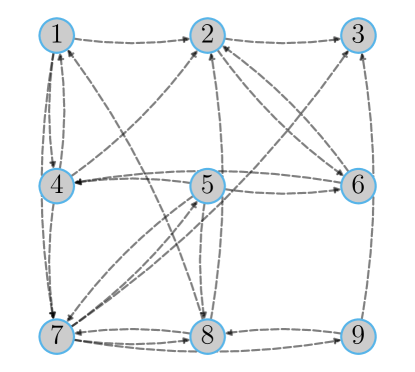
Figure 2: Topology of the communication network.

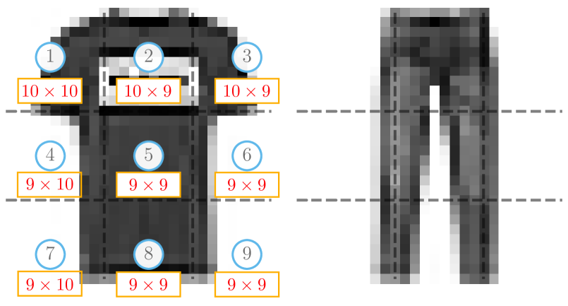
Figure 3: Observation map for 9 agents in the binary classification tasks with the FashionMNIST dataset.

VII-A FashionMNIST dataset

Each image of this dataset contains 784 ($28\times 28$) pixels. These pixels are assumed to be distributed as evenly as possible among the 9 agents in the network. We build a binary classification problem to distinguish “T-shirt” (labeled with $+1$) from “trouser” (labeled with $-1$). An example of each class and the size of the partial image observed by each agent are shown in Fig. 3. In the training phase, each agent trains its own classifier, which is a feedforward neural network with one hidden layer of $n_{1}$ neurons and activation function $\tanh$. For a given feature vector $h$ with dimension $d$, we denote the input to the outer layer by the vector $z=(z_{1},z_{2})$: $\forall m=1,2$,

$$z_{m}=\sum_{i=1}^{n_{1}}W_{im}^{(1)}\tanh(\sum_{j=1}^{d}W_{ji}^{(0)}h_{j}-\theta_{i}^{(0)})-\theta_{m}^{(1)}$$ (77)

where $W^{(0)}\in\mathbb{R}^{d\times n_{1}}$, $\theta^{(0)}\in\mathbb{R}^{n_{1}}$ (or $W^{(1)}\in\mathbb{R}^{n_{1}\times 2}$, $\theta^{(1)}\in\mathbb{R}^{2}$) are the weight matrix and the bias vector for the hidden (or output) layer, respectively. The final output is given by applying the $\operatorname*{softmax}$ function to $z$, which is expressed by

$$\widehat{p}(+1|h)=\frac{e^{z_{1}}}{e^{z_{1}}+e^{z_{2}}},\quad\widehat{p}(-1|h)=\frac{e^{z_{2}}}{e^{z_{1}}+e^{z_{2}}}.$$ (78)

where $\widehat{p}(+1|h)$ and $\widehat{p}(+1|h)$ are the estimated posteriors for the input $h$. In this case, the logit function (i.e., $c_{k}(h)$ in (2)) is approximated by:

$$f_{k}^{\sf NN}(h)\triangleq\log\frac{\widehat{p}(+1|h)}{\widehat{p}(-1|h)}=z_{1}-z_{2},$$ (79)

which belongs to the function class $\mathcal{F}_{k}^{\sf NN}$ that is parameterized by the weight matrices and bias vectors. In our simulations, we set $n_{1}=15$. This simple structure is employed in order to better visualize the probability of error curves. To illustrate the $\delta$-margin consistent training condition, we consider different sizes of training sets. For simplicity, we assume an identical training size for all agents, i.e., $N_{k}=N_{0},\forall k\in\mathcal{K}$. Given the value of $N_{0}$, a balanced training set is generated by randomly sampling from the FashionMNIST dataset. For each selected training set, the training is run using mini-batch iterates of 10 samples over 30 epochs. We employ the logistic loss in our simulations. The Adam optimizer [43] with learning rate 0.0001 is adopted.

In Fig. 4, we show the decision margins achieved under different training set sizes $N_{0}$, where the results are averaged over 200 different randomly generated training sets for each $N_{0}$. It can be observed that on average, the decision margin achieved in the training phase increases as $N_{0}$ grows. This indicates that with more training samples, a better learning condition (with better trained classifiers) is obtained for the prediction phase in our simulations. Next, we investigate the learning performance of the SML strategy for the statistical classification task. In our simulations, the underlying class for all observations is set to be “T-shirt”. For each training set considered in Fig. 4, we conduct 5000 Monte Carlo runs of statistical classification based on the trained classifiers associated with this training set and obtain the averaged result. The simulation result for a specified training set size $N_{0}$ is then estimated empirically from the associated 200 training sets.

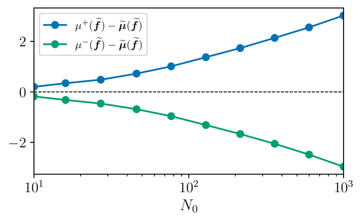
Figure 4: Decision margin under different sizes of training sets with the FashionMNIST dataset.

For performance comparison, we introduce the classical AdaBoost strategy where the $9$ agents are trained sequentially and their hard decisions are combined according to the accuracy attained by each local classifier [38]. Different from the SML strategy that aggregates the information over time following the social learning rule (16), AdaBoost ignores the temporal dependence in the true label among the unlabeled samples. Let $\widetilde{\bm{f}}_{k}^{\sf Boost}$ denote the model learned by agent $k$ in the training phase of AdaBoost, then the decision made by agent $k$ at time instant $i$, denoted by $\bm{\gamma}_{k,i}^{\sf Boost}$, is expressed as

$$\bm{\gamma}_{k,i}^{\sf Boost}=\operatorname*{sign}\Big{(}\widetilde{\bm{f}}_{k}^{\sf Boost}(\bm{h}_{k,i})\Big{)}.$$ (80)

The AdaBoost strategy is implemented in a centralized manner, which combines the local hard decisions from each agent and generates the prediction at time instant $i$ according to:

$$\bm{\gamma}_{i}^{\sf Boost}=\operatorname*{sign}\Bigg{(}\sum_{k=1}^{K}a_{k}\bm{\gamma}_{k,i}^{\sf Boost}\Bigg{)}$$ (81)

where $a_{k}$ is the classification accuracy for the training set that is achieved by agent $k$. In Fig. 5, we show the learning performance of agent $1$ in the SML strategy and that of the centralized decision $\bm{\gamma}_{i}^{\sf Boost}$ in AdaBoost for the statistical classification task. The evolution of the instantaneous probability of error $P_{1,i}^{e}$ for $i\in[0,30]$ under different $N_{0}$ is presented. We can see that for all training set sizes, $P_{1,i}^{e}$ decreases over time $i$ (i.e., the number of observations collected so far). For larger $N_{0}$, the decaying is almost exponential and the decay rate is positively correlated to the decision margin as indicated by Fig. 4, which is consistent with (56) in Theorem 1. In contrast to it, due to the lack of information aggregation over time, the probability of error attained by the centralized AdaBoost strategy remains invariant as more prediction samples are collected. Particularly, for each training set size $N_{0}$, the SML strategy outperforms the AdaBoost when more than two unlabeled samples are collected. This reveals a distinct advantage of the SML strategy in the prediction accuracy for the statistical classification tasks.

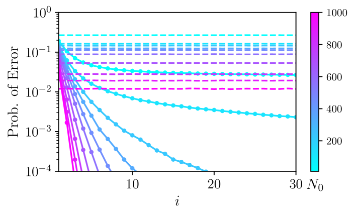
Figure 5: Statistical classification task: Evolution of the probability of error within the SML strategy (dotted lines) and AdaBoost (dashed lines) over the prediction samples $i$ for different training set sizes $N_{0}$ with the FashionMNIST dataset.

Finally, we investigate the learning performance of the SML strategy, represented by the ensemble classifier (71), for the single-sample classification task. According to Theorem 2, the probability of error with this task can be upper bounded by a constant relevant to the decision margin $\delta$. In view of Fig. 4, the probability of error is expected to be reduced with more training samples. This is consistent with the curve of $P_{e}$ in Fig. 6, where the result for each $N_{0}$ is averaged over the 200 training sets of size $N_{0}$. Meanwhile, we compare the classification error of the SML strategy to that of the non-cooperative scenario where each agent predicts according to their own trained classifiers $\widetilde{\bm{c}}_{k}$, and to that of the centralized AdaBoost strategy. As observed in Fig. 6, the collaboration in the prediction phase helps the agents, especially those with poorly trained classifiers, learn a better decision rule for the simulated classification tasks. Furthermore, we can see that the SML strategy outperforms AdaBoost when $N_{0}$ is small. Since the local classifiers are trained sequentially in AdaBoost, this observation implies that the cooperative training is not helpful for prediction when the number of training samples is limited. This phenomenon can be explained by the fact that the agents are heterogeneous in our simulated distributed setting. The heterogeneity of agents is manifested in two aspects: (i) each agent observes a different part of the whole image, and (ii) the dimension of the feature vectors received by each agent is varying and thus the structure of the local classifier differs. Due to the diversity of information within the agent’s local training sets, it may not be a wise choice for the agent to place more weights on the training samples that have been misclassified by the previously trained agents when the number of training samples is limited. As the size of the training set increases, this adverse effect is mitigated and consequently, the classification accuracy of AdaBoost becomes close to that of the SML strategy. Fig. 6 has an important implication on the classification tasks involving multiple classifiers: it is essential to take into account the heterogeneity of the information before implementing cooperative training.

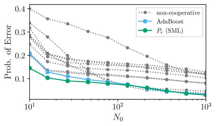
Figure 6: Single-sample classification task: Probability of error of non-cooperative agents (dotted lines) and of the cooperative SML strategy (green line) and the centralized AdaBoost (blue line) with the FashionMNIST dataset.

VII-B CIFAR10 dataset

The images in CIFAR10 dataset are of size $3\times 32\times 32$, that is, they are 3-channel color images of $32\times 32$ pixels in size. We consider the binary classification problem to distinguish “cats” from “dogs” within this dataset. An example for each of the selected two classes and the sizes of the partial image observed by each agent are shown in Fig. 7. A convolutional neural network composed of two convolutional layers with activation function $\operatorname*{ReLu}$, followed by max-pooling layers and three fully connected layers with activation function $\tanh$, is employed by the agents. Since each agent observes a partial image with a slightly different size, we assume that they use a different kernel size in the first convolutional layer such that the output size of this layer is equal to $6\times 8\times 8$. A max-pooling layer with size 2 and stride 2 follows and reduces the output size to $6\times 4\times 4$. The second convolutional layer has 16 channels and a kernel size $(2,2)$, followed by a max-pooling layer with size 2 and stride 1, which finally generates an input feature vector of dimension 64 ($16\times 2\times 2$) to the subsequent fully connected layers. The three fully connected layers can be viewed as a feedforward neural network with two hidden layers of sizes 32 and 15, respectively. It is not easy to tell the difference between cats and dogs within this dataset and a classification accuracy around $65\%$ is attained by the specified convolutional neural network when the agents can observe the whole image and use all 10000 training samples provided by the dataset. In our simulations, the training is run using a mini-batch of 128 samples over 100 epochs. The setting of the loss function and the optimizer as well as the learning rate is the same as that for the FashionMNIST dataset.

In Fig. 8, we present the decision margins achieved by the network under different training set sizes $N_{0}$. Except for the case of $N_{0}=10000$ where all training samples of the selected classes are utilized, 200 different training sets are generated randomly for each other $N_{0}$ to obtain the averaged result. It is obvious from Fig. 8 that in general, a better margin condition is achieved with more labeled samples in the training phase. Whereas, the decision margins attained in Fig. 8 are much smaller than those shown in Fig. 4. This implies that for the specified classifiers, distinguishing cats from dogs within the CIFAR10 dataset is much harder than distinguishing T-shirts from trousers within the FashionMNIST dataset.

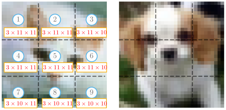
Figure 7: Observation map for 9 agents in the binary classification tasks with the CIFAR10 dataset.

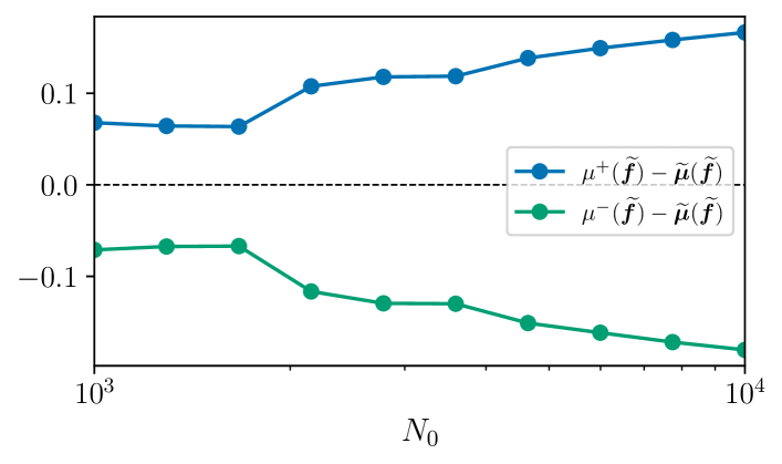
Figure 8: Decision margin under different sizes of training sets with the CIFAR10 dataset.

For the statistical classification task where the true class is “cat”, the instantaneous probability of error associated with agent $1$ within the SML strategy and that of the centralized AdaBoost strategy are presented in Fig. 9. As the number of observations grows, an exponential decay of the misclassification error within the SML strategy is observed for each $N_{0}$ in the simulations. Meanwhile, the decay rate becomes larger when the decision margin is increased with more training samples available for the training phase. Compared to AdaBoost, the SML strategy exhibits a significant advantage in prediction accuracy by effectively leveraging the temporal dependence in the true label of the streaming unlabeled samples. Specially, agent $1$ is able to make a better decision within two iterations by employing the social learning rule (16).

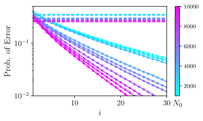
Figure 9: Statistical classification task: Evolution of the probability of error within the SML strategy (dotted lines) and AdaBoost (dashed lines) over the prediction samples $i$ for different training set sizes $N_{0}$ with the CIFAR10 dataset.

Finally, we compare the classification errors of the distributed SML strategy, the centralized AdaBoost strategy, and the non-cooperative scenario in the single-sample classification task. The results are shown in Fig. 10. It can be observed that the ensemble classifier (71) formulated by the SML strategy, improves the prediction accuracy for all agents working in the non-cooperative scenario. This demonstrates the effectiveness of a cooperative decision-making for solving the binary classification task under consideration. Moreover, for each training set size $N_{0}$, the distributed SML strategy shows a comparable performance to the centralized AdaBoost strategy. Since the training process for the local classifiers is fully independent in the SML strategy, this strategy is easier to be implemented in practice.

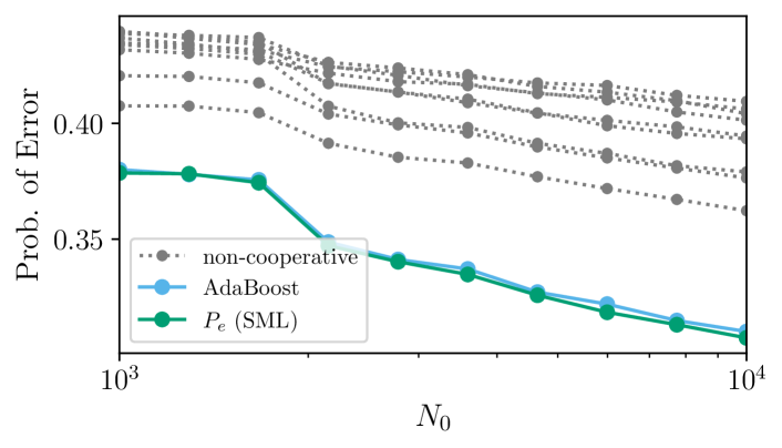
Figure 10: Single-sample classification task: Probability of error of non-cooperative agents (dotted lines) and of the cooperative SML strategy (green line) and the centralized AdaBoost (blue line) with the CIFAR10 dataset.

VIII Concluding remarks

This paper studies the learning performance of the social machine learning strategy, which is a fully data-driven distributed decision-making architecture. For two binary classification problems with limited number of samples for inference in the prediction phase, we derived an upper bound on the corresponding probability of error. Our results extend the analysis in [9], which investigated the classification error when the number of observations grows indefinitely. There are still many interesting open questions regarding the performance of the social machine learning strategy. As indicated in [9], this strategy can be formulated to address multi-class classification tasks. However, the theoretical guarantees in this case are more involved than the binary case, Specifically, the $\delta$-consistent training condition becomes more intricate, and the analytical methodology to derive the lower bound (Lemma 2) needs to be developed. The performance analysis for multi-class classification tasks will be considered in future work.

Appendices

A Proofs of Lemmas 1 and 2

Since the consistent training condition (22) corresponds to the case $\delta=0$ in the $\delta$-margin consistent training condition (47), we will focus on the proof of Lemma 2 in the following. First, we recall some important results on the estimation errors of the empirical risk and the training mean, which have been established in [9].

Lemma A (Theorem 3 in [9]).

Under Assumptions 1 and 2, we have the following two results. First,

$$\mathbb{P}\left(\sup_{f\in\mathcal{F}}\absolutevalue{\widetilde{\bm{R}}(f)-R(f)}\geq x\right)\leq\exp\left\{-\frac{N_{\max}(x-4L_{\phi}\rho)}{2\alpha^{2}L_{\phi}^{2}\beta^{2}}\right\},$$ (82)

for any $x>4L_{\phi}\rho$, where $\mathcal{F}\triangleq\mathcal{F}_{1}\times\mathcal{F}_{2}\cdots\times\mathcal{F}_{K}$. Second,

$$\mathbb{P}\left(\sup_{f\in\mathcal{F}}\absolutevalue{\widetilde{\bm{\mu}}(f)-\mu(f)}\geq x\right)\leq\exp\left\{-\frac{N_{\max}(x-4\rho)^{2}}{2\alpha^{2}\beta^{2}}\right\},$$ (83)

for any $x>4\rho$, where

$$\mu(f)=\frac{\mu^{+}(f)+\mu^{-}(f)}{2},\quad\forall f\in\mathcal{F}.$$ (84)

We will also use the following property related to strictly monotonic functions and their inverse functions [44].

Property 1 (Inverse of strictly monotone function [44]).

Let $f$ be a real function defined on $I\subseteq\mathbb{R}$ whose image is $J\subseteq\mathbb{R}$. Assume that $f$ is strictly monotone on $I$, then $f$ always has an inverse function $f^{-1}$ that has the same monotonicity as $f$. That is, if $f$ is strictly increasing (or decreasing), then so is $f^{-1}$.

In order to establish Lemma 2, we need to upper bound the probability $1-P_{c,\delta}$ with the following inequality:

$$\;1-P_{c,\delta}$$

$$=\mathbb{P}\left(\left\{\mu^{+}(\widetilde{\bm{f}})\leq\widetilde{\bm{\mu}}({\widetilde{\bm{f}}})+\delta\right\}\cup\left\{\mu^{-}(\widetilde{\bm{f}})\geq\widetilde{\bm{\mu}}(\widetilde{\bm{f}})-\delta\right\}\right)$$

$$=\mathbb{P}\left(\left\{\mu^{+}(\widetilde{\bm{f}})-\mu(\widetilde{\bm{f}})\leq\widetilde{\bm{\mu}}(\widetilde{\bm{f}})-\mu(\widetilde{\bm{f}})+\delta\right\}\right.$$

$$\qquad\quad\left.\cup\left\{\mu^{-}(\widetilde{\bm{f}})-\mu(\widetilde{\bm{f}})\geq\widetilde{\bm{\mu}}(\widetilde{\bm{f}})-\mu(\widetilde{\bm{f}})-\delta\right\}\right)$$

$$\overset{\textnormal{(a)}}{=}\mathbb{P}\left(\absolutevalue{\widetilde{\bm{\mu}}(\widetilde{\bm{f}})-\mu(\widetilde{\bm{f}})}\geq\frac{\mu^{+}(\widetilde{\bm{f}})-\mu^{-}(\widetilde{\bm{f}})}{2}-\delta\right)$$

$$\leq\mathbb{P}\left(\absolutevalue{\widetilde{\bm{\mu}}(\widetilde{\bm{f}})-\mu(\widetilde{\bm{f}})}\geq d-\delta\right)$$

$$\quad+\mathbb{P}\left(\frac{\mu^{+}(\widetilde{\bm{f}})-\mu^{-}(\widetilde{\bm{f}})}{2}\leq d\right)$$ (85)

for any $d>\delta$, where (a) comes from the definition of $\mu(\widetilde{\bm{f}})$ in (84). Using Lemma A, the first term of (85) satisfies

$$\;\mathbb{P}\left(\absolutevalue{\widetilde{\bm{\mu}}(\widetilde{\bm{f}})-\mu(\widetilde{\bm{f}})}\geq d-\delta\right)$$

$$\leq\mathbb{P}\left(\sup_{f\in\mathcal{F}}\absolutevalue{\widetilde{\bm{\mu}}(f)-\mu(f)}\geq d-\delta\right)$$

$$\leq\exp\left\{-\frac{N_{\max}(d-\delta-4\rho)^{2}}{2\alpha^{2}\beta^{2}}\right\}$$ (86)

for all $d>4\rho+\delta$. The bound on the second term of (85) can be established based on Assumption 1 and Jensen’s inequality. Given the function $f_{k}\in\mathcal{F}_{k}$ for each $k\in\mathcal{K}$, the network average of the expected risks evaluated on the training samples $(\widetilde{\bm{h}}_{k,n},\widetilde{\bm{\gamma}}_{k,n})$ is bounded as follows:

$$R(f) \overset{\eqref{eq: network average for the expected risk}}{=}\sum_{k=1}^{K}\pi_{k}\mathbb{E}_{\widetilde{h}_{k},\widetilde{\gamma}}\phi\left(\widetilde{\bm{\gamma}}_{k,n}f_{k}(\widetilde{\bm{h}}_{k,n})\right)$$

$$\overset{\textnormal{(a)}}{\geq}\sum_{k=1}^{K}\pi_{k}\phi\left(\mathbb{E}_{\widetilde{h}_{k},\widetilde{\gamma}}\widetilde{\bm{\gamma}}_{k,n}f_{k}(\widetilde{\bm{h}}_{k,n})\right)$$

$$\overset{\textnormal{(b)}}{\geq}\phi\left(\sum_{k=1}^{K}\pi_{k}\mathbb{E}_{\widetilde{h}_{k},\widetilde{\gamma}}\widetilde{\bm{\gamma}}_{k,n}f_{k}(\widetilde{\bm{h}}_{k,n})\right)$$

$$\overset{\textnormal{(c)}}{=}\phi\left(\frac{1}{2}\sum_{k=1}^{K}\pi_{k}\mathbb{E}_{+1}f_{k}(\widetilde{\bm{h}}_{k,n})-\frac{1}{2}\sum_{k=1}^{K}\pi_{k}\mathbb{E}_{-1}f_{k}(\widetilde{\bm{h}}_{k,n})\right)$$

$$\overset{\textnormal{(d)}}{=}\phi\left(\frac{\mu^{+}(f)-\mu^{-}(f)}{2}\right),$$ (87)

where in (a) and (b) we used Jensen’s inequality with the convex function $\phi$. In (c), we used the uniform prior assumption of the training samples, and in (d) we used the definition of conditional means (19). We recall that the notation $\mathbb{E}_{\gamma}$ denotes the expectation operator associated with the likelihood models $L_{k}(\cdot|\gamma)$ for $\gamma\in\Gamma$. From (87) and the non-increasing property of $\phi$, we know that for any given function $f\in\mathcal{F}$:

$$\frac{\mu^{+}(f)-\mu^{-}(f)}{2}\leq d\Rightarrow R(f)\geq\phi(d).$$ (88)

Replacing the generic $f$ with the trained function $\widetilde{\bm{f}}$ obtained from the empirical risk minimization (5), we have

$$\mathbb{P}\left(\frac{\mu^{+}(\widetilde{\bm{f}})-\mu^{-}(\widetilde{\bm{f}})}{2}\leq d\right)\leq\mathbb{P}\left(R(\widetilde{\bm{f}})\geq\phi(d)\right).$$ (89)

The probability on the right-hand side can be bounded using the uniform bound on the estimation error for the empirical risk (82). First, we develop the following inequality:

$$R(\widetilde{\bm{f}})-\mathsf{R}^{o} \overset{\textnormal{(a)}}{=}R(\widetilde{\bm{f}})-\inf_{f\in\mathcal{F}}R(f)$$

$$=R(\widetilde{\bm{f}})-\widetilde{\bm{R}}(\widetilde{\bm{f}})+\widetilde{\bm{R}}(\widetilde{\bm{f}})-\inf_{f\in\mathcal{F}}R(f)$$ (90)

$$=R(\widetilde{\bm{f}})-\widetilde{\bm{R}}(\widetilde{\bm{f}})+\sup_{f\in\mathcal{F}}\left(\widetilde{\bm{R}}(\widetilde{\bm{f}})-R(f)\right)$$

$$\overset{\textnormal{(b)}}{\leq}R(\widetilde{\bm{f}})-\widetilde{\bm{R}}(\widetilde{\bm{f}})+\sup_{f\in\mathcal{F}}\left(\widetilde{\bm{R}}(f)-R(f)\right)$$

$$\leq 2\sup_{f\in\mathcal{F}}\absolutevalue{\widetilde{\bm{R}}(f)-R(f)}$$ (91)

where (a) follows directly from the definition of $\mathsf{R}^{o}$ in (25), while (b) is based on the definitions of $\widetilde{\bm{f}}_{k}$ and $\bm{R}(f)$ in (4) and (30) respectively, which ensure that $\widetilde{\bm{R}}(\widetilde{\bm{f}})\leq\widetilde{\bm{R}}(f)$. Therefore, one gets

$$\mathbb{P}\left(R(\widetilde{\bm{f}})\geq\phi(d)\right) =\mathbb{P}\left(R(\widetilde{\bm{f}})-\mathsf{R}^{o}\geq\phi(d)-\mathsf{R}^{o}\right)$$

$$\overset{\textnormal{(a)}}{\leq}\mathbb{P}\left(\sup_{f\in\mathcal{F}}\absolutevalue{\widetilde{\bm{R}}(f)-R(f)}\geq\frac{\phi(d)-\mathsf{R}^{o}}{2}\right)$$

$$\overset{\textnormal{(b)}}{\leq}\exp\left\{-\frac{N_{\max}\Big{(}\frac{\phi(d)-\mathsf{R}^{o}}{2}-4L_{\phi}\rho\Big{)}}{2\alpha^{2}L_{\phi}^{2}\beta^{2}}\right\}$$ (92)

for any $d$ such that $\frac{\phi(d)-\mathsf{R}^{o}}{2}>4L_{\phi}\rho$, where (a) comes from (91) and (b) is derived using (82) in Lemma A.

According to (85), by combining (86), (89), and (92), we have

$$P_{c,\delta} \geq 1-\mathbb{P}\left(\absolutevalue{\widetilde{\bm{\mu}}(\widetilde{\bm{f}})-\mu(\widetilde{\bm{f}})}\geq d-\delta\right)$$

$$\quad\;-\mathbb{P}\left(\frac{\mu^{+}(\widetilde{\bm{f}})-\mu^{-}(\widetilde{\bm{f}})}{2}\leq d\right)$$

$$\geq 1-\exp\left\{-\frac{N_{\max}(d-\delta-4\rho)^{2}}{2\alpha^{2}\beta^{2}}\right\}$$

$$\quad\;-\exp\left\{-\frac{N_{\max}\Big{(}\frac{\phi(d)-\mathsf{R}^{o}}{2}-4L_{\phi}\rho\Big{)}^{2}}{2\alpha^{2}L_{\phi}^{2}\beta^{2}}\right\}$$ (93)

for any $d$ contained in the following interval:

$$d\in(4\rho+\delta,d_{\max})$$ (94)

where $d_{\max}$ is defined by

$$d_{\max}\triangleq\sup\left\{x:\phi(x)=\mathsf{R}^{o}+8L_{\phi}\rho\right\}.$$ (95)

If the loss function $\phi$ is strictly monotonic, then from Property 1, $\phi$ has an inverse function $\phi^{-1}$ and $d_{\max}$ can be written as

$$d_{\max}=\phi^{-1}(\mathsf{R}^{o}+8L_{\phi}\rho).$$ (96)

Observe that the leading coefficients of the exponents in (93) are equal when

$$d-\delta-4\rho=\frac{\phi(d)-\mathsf{R}^{o}}{2L_{\phi}}-4\rho,$$ (97)

which yields

$$\phi(d)-\mathsf{R}^{o}-2L_{\phi}(d-\delta)=0.$$ (98)

Define $g(d)$ as the following function of variable $d$:

$$g(d)\triangleq d-\frac{\phi(d)-\mathsf{R}^{o}}{2L_{\phi}}.$$ (99)

For a given decision margin $\delta\geq 0$, let $d_{\delta}^{\star}$ denote a solution to the equation $g(d)=\delta$, i.e.,

$$g(d_{\delta}^{\star})=\delta.$$ (100)

If we can prove that $d_{\delta}^{\star}>\delta$, then from (93), the probability of $\delta$-consistent training $P_{c,\delta}$ can be lower bounded as

$$P_{c,\delta}\geq 1-2\exp\left\{-\frac{8N_{\max}\Big{(}\frac{d_{\delta}^{\star}-\delta}{4}-\rho\Big{)}^{2}}{\alpha^{2}\beta^{2}}\right\}$$ (101)

when the Rademacher complexity $\rho$ satisfies $\rho<\frac{d_{\delta}^{\star}-\delta}{4}$. Let

$$\mathdutchcal{E}(\mathsf{R}^{o},\delta)\triangleq\frac{d_{\delta}^{\star}-\delta}{4}.$$ (102)

In the following, we prove that such constant $d_{\delta}^{\star}$ exists when the margin $\delta$ is small, i.e., $\mathdutchcal{E}(\mathsf{R}^{o},\delta)>0$ for a small $\delta$.

First, we notice that due to the non-increasing property of $\phi$ (Assumption 1), $g(d)$ is a strictly increasing function of $d$. This implies that for any $\delta>0$, the solution $d_{\delta}^{\star}$ (100) is unique. Furthermore, $\phi$ is differentiable at $0$ and $\phi^{\prime}(0)<0$ under Assumption 1. With the condition $\mathsf{R}^{o}<\phi(0)$ in (27), we have

$$g(0)=-\frac{\phi(0)-\mathsf{R}^{o}}{2L_{\phi}}<0.$$ (103)

Since $g(d)$ is increasing, we know that the equation $g(d)=\delta$ has a positive solution for the case $\delta=0$. That is, $\exists d_{0}^{\star}>0$ such that $g(d_{0}^{\star})=0$. Due to the strict monotonicity of $g(d)$, we know that according to Property 1, there is an inverse function $g^{-1}$ which is strictly increasing. Therefore, for any $\delta>0$, the equation $g(d)=\delta$ has a unique positive solution $d_{\delta}^{\star}=g^{-1}(\delta)$. Moreover, $d_{\delta}^{\star}$ increases with a larger margin $\delta$. Let

$$d_{\mathsf{R}}\triangleq\inf\left\{x:\phi(x)=\mathsf{R}^{o}\right\}$$ (104)

be the infimum of the set of $x$ corresponding to the target risk $\mathsf{R}^{o}$. Particularly, if $\phi$ is strictly decreasing, we have $d_{\mathsf{R}}=\phi^{-1}(\mathsf{R}^{o})$. It is clear from $\eqref{eq: R^o condition}$ that $d_{\mathsf{R}}>0$. By definition in $d_{\delta}^{\star}$ (100), we get

$$\mathdutchcal{E}(\mathsf{R}^{o},\delta)=\frac{d_{\delta}^{\star}-\delta}{4}=\frac{\phi(d_{\delta}^{\star})-\mathsf{R}^{o}}{8L_{\phi}}.$$ (105)

Therefore, $\mathdutchcal{E}(\mathsf{R}^{o},\delta)>0$ if, and only if, $\phi(d_{\delta}^{\star})>\mathsf{R}^{o}$. In other words, the lower bound provided by (101) is meaningful if, and only if, $d_{\delta}^{\star}<d_{\mathsf{R}}$. Since $d_{\delta}^{\star}$ is increasing with $\delta$, the margin $\delta$ must be selected to be smaller than a constant $\delta_{\max}$ whose definition is

$$\delta_{\max}\triangleq\sup\left\{\delta\geq 0:g(d)=\delta\text{ has a solution }d_{\delta}^{\star}<d_{\mathsf{R}}\right\}.$$ (106)

The existence of the constant $\delta_{\max}$ is guaranteed by the strict monotonicity of function $g$. Therefore, (101) holds for any $\delta<\delta_{\max}$ and $\rho<\mathdutchcal{E}(\mathsf{R}^{o},\delta)$. This proves (49) in Lemma 2.

Since our proof does not require $\delta$ to be strictly greater than 0, the above analysis applies also to the case $\delta=0$, i.e., the case of consistent training (22). Let $\delta=0$ in (102), we have

$$\mathdutchcal{E}(\mathsf{R}^{o},0)=\frac{d_{0}^{\star}}{4}.$$ (107)

In addition, we can establish the following relation for $\mathdutchcal{E}(\mathsf{R}^{o},\delta)$ under consistent training and $\delta$-margin consistent training:

$$\mathdutchcal{E}(\mathsf{R}^{o},\delta) \overset{\text{(a)}}{=}\frac{\phi(d_{\delta}^{\star})-\mathsf{R}^{o}}{8L_{\phi}}$$

$$=\frac{\phi(d_{\delta}^{\star})-\phi(d_{0}^{\star})}{8L_{\phi}}+\frac{\phi(d_{0}^{\star})-\mathsf{R}^{o}}{8L_{\phi}}$$

$$\overset{\text{(b)}}{\leq}\frac{\phi(d_{0}^{\star})-\mathsf{R}^{o}}{8L_{\phi}}=\mathdutchcal{E}(\mathsf{R}^{o},0)$$ (108)

where (a) follows from (105) and (b) is due to $d_{\delta}^{\star}\geq d_{0}^{\star}$ and the non-increasing property of $\phi$. As expected, the lower bound on the probability of $\delta$-consistent training benefits from an increasing margin $\delta$. The proofs of Lemmas 1 and 2 are complete.

B Proof of Theorem 1

The proof is based on McDiarmid’s inequality [45, 3] stated in the following Lemma.

Lemma B (McDiarmid’s inequality).

Let $\bm{x}$ represent a sequence of independent random variables $\bm{x}_{n}$, with $n=1,2,\dots,N$ and $\bm{x}_{n}\in\mathcal{X}_{n}$ for all $n$. Suppose that the function $g$: $\prod_{n=1}^{N}\mathcal{X}_{n}\mapsto\mathbb{R}$ satisfies for every $n=1,2,\dots,N$:

$$\absolutevalue{g(x)-g(\widehat{x})}\leq b_{n}$$ (109)

whenever the sequences $x$ and $\widehat{x}$ differ only in the $n$-th component. Then, for any $\varepsilon>0$:

$$\mathbb{P}\left(g(\bm{x})-\mathbb{E}g(\bm{x})\geq\varepsilon\right)\leq\exp(-\frac{2\varepsilon^{2}}{\sum_{n=1}^{N}b_{n}^{2}}),$$ (110)

$$\mathbb{P}\left(g(\bm{x})-\mathbb{E}g(\bm{x})\leq-\varepsilon\right)\leq\exp(-\frac{2\varepsilon^{2}}{\sum_{n=1}^{N}b_{n}^{2}}).$$ (111)

We also need the following result on the convergence of matrix powers in the proof.

Lemma C (Convergence of matrix powers [13]).

Consider a strongly-connected network of $K$ agents and a left-stochastic combination policy $A$. Let $0\leq\sigma<1$ denote the second largest-magnitude eigenvalue of $A$. Then, for any $t$ and for any agent $k$, the following inequality holds:

$$\sum_{\tau=1}^{t}\sum_{\ell=1}^{K}\absolutevalue{[A^{t-\tau}]_{\ell k}-\pi_{\ell}}\leq\frac{4\log K}{1-\sigma}$$ (112)

Before proving Theorem 1, it is worth noting that the approximate logit functions $\widetilde{\bm{f}}_{k}$ and the corresponding trained classifiers $\widetilde{\bm{c}}_{k}$ are random w.r.t. the training samples $(\widetilde{\bm{h}}_{k,n},\widetilde{\bm{\gamma}}_{k,n})$. Since the training phase is independent of the prediction phase within the SML framework, the randomness stemming from the training phase can be “frozen” when we develop our analysis for the prediction phase. Particularly, for any observation $\bm{h}_{k,i}$ in the prediction phase, both $\widetilde{\bm{f}}_{k}(\bm{h}_{k,i})$ and $\widetilde{\bm{c}}_{k}(\bm{h}_{k,i})$ are deterministic values since the expressions of $\widetilde{\bm{f}}_{k}$ and $\widetilde{\bm{c}}_{k}$ have been specified in the training phase. To eliminate any potential ambiguity, in this proof, we will employ normal fonts for random variables that are independent of the prediction phase. For example, we will use the notation $\widetilde{{f}}_{k}$ and $\widetilde{{c}}_{k}$ instead of $\widetilde{\bm{f}}_{k}$ and $\widetilde{\bm{c}}_{k}$ throughout this proof. However, we keep the symbol $\sim$ on top of variables related to the training phase.

Our proof proceeds as follows. We begin with the case where the true state of the statistical classification task is $+1$, namely, $\bm{\gamma}_{0}=+1$. According to the distributed learning rule (16), the log-belief ratio of agent $k$ at time $i$ is expressed by

$$\bm{\lambda}_{k,i}\overset{\eqref{eq: sl learning rule}}{=} \sum_{\ell=1}^{K}a_{\ell k}\left(\bm{\lambda}_{\ell,i-1}+\widetilde{{c}}_{\ell}({\bm{h}}_{\ell,i})\right)$$

$$= \sum_{\ell=1}^{K}[A^{i}]_{\ell k}\bm{\lambda}_{\ell,0}+\sum_{\tau=1}^{i}\sum_{\ell=1}^{K}[A^{i+1-\tau}]_{\ell k}\widetilde{{c}}_{\ell}(\bm{h}_{\ell,\tau}).$$ (113)

Under the uniform initial belief condition, i.e., $\bm{\lambda}_{\ell,0}=0$ for all $\ell\in\mathcal{K}$, we get

$$\bm{\lambda}_{k,i}=\sum_{\tau=1}^{i}\sum_{\ell=1}^{K}[A^{i+1-\tau}]_{\ell k}\widetilde{{c}}_{\ell}(\bm{h}_{\ell,\tau}).$$ (114)

First, we show that the expectation of $\bm{\lambda}_{k,i}$ is lower bounded by the upcoming equation (118). Taking the expectation of (114) w.r.t. the historical observations received by the network until time $i$, we have

$$\mathbb{E}_{+1}{\bm{\lambda}_{k,i}} =\mathbb{E}_{+1}\left[\sum_{\tau=1}^{i}\sum_{\ell=1}^{K}[A^{i+1-\tau}]_{\ell k}\widetilde{{c}}_{\ell}(\bm{h}_{\ell,\tau})\right]$$

$$\overset{\text{(a)}}{=}\sum_{\tau=1}^{i}\sum_{\ell=1}^{K}[A^{i+1-\tau}]_{\ell k}\mathbb{E}_{+1}\left[\widetilde{{c}}_{\ell}(\bm{h}_{\ell,\tau})\right]$$

$$\overset{\text{(b)}}{=}\sum_{\tau=1}^{i}\sum_{\ell=1}^{K}[A^{i+1-\tau}]_{\ell k}(\mu_{\ell}^{+}(\widetilde{{f}}_{\ell})-\widetilde{{\mu}}_{\ell}(\widetilde{{f}}_{\ell}))$$

$$\overset{\text{(c)}}{=}\sum_{\tau=1}^{i}\sum_{\ell=1}^{K}\left([A^{i+1-\tau}]_{\ell k}-\pi_{\ell}\right)(\mu_{\ell}^{+}(\widetilde{{f}}_{\ell})-\widetilde{{\mu}}_{\ell}(\widetilde{{f}}_{\ell}))$$

$$\quad+i(\mu^{+}(\widetilde{{f}})-\widetilde{{\mu}}(\widetilde{{f}}))$$ (115)

where in (a) we used the independence of local observations across time (i.e., $\tau$) and space (i.e., $\ell$) conditioned on the true state $\bm{\gamma}_{0}$, and in (b) we used the assumption of $\bm{\gamma}_{0}=+1$. In (c) we used the definitions of $\mu^{+}(\widetilde{{f}})$ and $\widetilde{{\mu}}(\widetilde{{f}})$ in (21) and (23). With the bound of $f_{k}$ specified in Assumption 2, we get

$$\absolutevalue{\mu_{\ell}^{+}(\widetilde{{f}}_{\ell})-\widetilde{{\mu}}_{\ell}(\widetilde{{f}}_{\ell})}\leq 2\beta.$$ (116)

In view of the convergence of matrix powers (112) in Lemma C, we have

$$\;\absolutevalue{\sum_{\tau=1}^{i}\sum_{\ell=1}^{K}\left([A^{i+1-\tau}]_{\ell k}-\pi_{\ell}\right)(\mu_{\ell}^{+}(\widetilde{{f}}_{\ell})-\widetilde{{\mu}}_{\ell}(\widetilde{{f}}_{\ell}))}$$

$$\overset{\textnormal{(a)}}{\leq}\sum_{\tau=1}^{i}\sum_{\ell=1}^{K}\absolutevalue{[A^{i+1-\tau}]_{\ell k}-\pi_{\ell}}\cdot\max_{\ell\in\mathcal{K}}\absolutevalue{\mu_{\ell}^{+}(\widetilde{{f}}_{\ell})-\widetilde{{\mu}}_{\ell}(\widetilde{{f}}_{\ell})}$$

$$\leq\frac{4\log K}{1-\sigma}\cdot 2\beta=\frac{8\beta\log K}{1-\sigma}=\kappa$$ (117)

where (a) follows from Hölder’s inequality [3], and $\kappa$ is defined in (55). Therefore, (115) is lower bounded by

$$\mathbb{E}_{+1}{\bm{\lambda}_{k,i}}\geq i(\mu^{+}(\widetilde{{f}})-\widetilde{{\mu}}(\widetilde{{f}}))-\kappa.$$ (118)

Next, we show that the boundedness of $f_{k}$ also ensures that the log-belief ratio $\bm{\lambda}_{k,i}$, as a function of the historical observations $\bm{h}_{\ell,\tau}$ with $\ell\in\mathcal{K}$ and $\tau\leq i$, satisfies the bounded difference condition (109). Let

$${\sf h}_{i}\triangleq\big{\{}\bm{h}_{k,\tau},\forall k\in\mathcal{K},\forall 1\leq\tau\leq i\big{\}}$$ (119)

denote the sequence of observations received by the network up to time $i$. For any given sequence ${\sf h}_{i}$, the log-belief ratio of agent $k$ at time $i$ is represented by $\bm{\lambda}_{k,i}({\sf h}_{i})$. Due to the independence of local observations, we know that ${\sf h}_{i}$ is composed of $Ki$ independent random variables $\bm{h}_{\ell,\tau}$ conditional on the underlying state. Now let us consider another sequence of observations $\widehat{\sf h}_{i}$ that differs from ${\sf h}_{i}$ only in $\bm{h}_{\ell,\tau}$, namely,

$$\widehat{\bm{h}}_{\ell^{\prime},\tau^{\prime}}=\bm{h}_{\ell^{\prime},\tau^{\prime}},\quad\forall\ell^{\prime}\neq\ell\textnormal{ and }\forall\tau^{\prime}\neq\tau.$$ (120)

The difference between $\bm{\lambda}_{k,i}({\sf h}_{i})$ and $\bm{\lambda}_{k,i}(\widehat{\sf h}_{i})$ is bounded as

$$\;\absolutevalue{\bm{\lambda}_{k,i}({\sf h}_{i})-\bm{\lambda}_{k,i}(\widehat{\sf h}_{i})}$$

$$\overset{\text{(a)}}{=}\absolutevalue{[A^{i+1-\tau}]_{\ell k}\widetilde{{c}}_{\ell}(\bm{h}_{\ell,\tau})-[A^{i+1-\tau}]_{\ell k}\widetilde{{c}}_{\ell}(\widehat{\bm{h}}_{\ell,\tau})}$$

$$\overset{\text{(b)}}{=}[A^{i+1-\tau}]_{\ell k}\absolutevalue{\widetilde{{f}}_{\ell}(\bm{h}_{\ell,\tau})-\widetilde{{f}}_{\ell}(\widehat{\bm{h}}_{\ell,\tau})}$$

$$\leq 2[A^{i+1-\tau}]_{\ell k}\beta$$ (121)

where (a) is due to (114) and (120), and (b) is due to the definition of $\widetilde{{c}}_{\ell}$ given in (7). The last inequality follows directly from Assumption 2. In terms of condition (109) in Lemma B, we denote the bound (121) associated with random variable $\bm{h}_{\ell,\tau}$ by $b_{\ell,i}(\tau)$:

$$b_{\ell,i}(\tau)\triangleq 2[A^{i+1-\tau}]_{\ell k}\beta.$$ (122)

The sum of variations involving $Ki$ independent random variables in $\bm{\lambda}_{k,i}({\sf h}_{i})$, which is necessary to apply McDiarmid’s inequalities, is bounded with

$$b_{k,i}\triangleq\sum_{\tau=1}^{i}\sum_{\ell=1}^{K}b_{\ell,i}(\tau)^{2} =\sum_{\tau=1}^{i}\sum_{\ell=1}^{K}{\left(2[A^{i+1-\tau}]_{\ell k}\beta\right)^{2}}$$

$$=4\beta^{2}\sum_{\tau=1}^{i}\sum_{\ell=1}^{K}[A^{i+1-\tau}]_{\ell k}^{2}$$

$$\leq 4\beta^{2}i$$ (123)

where the last inequality holds due to the stochastic matrix $A$. That is, the matrix power of a left-stochastic matrix still gives a left-stochastic matrix: $\forall m=1,2,\dots$,

$$\mathbbm{1}^{\top}A^{m}=\mathbbm{1}^{\top}A^{m-1}=\dots=\mathbbm{1}^{\top}A=\mathbbm{1}^{\top}$$ (124)

where $\mathbbm{1}$ is the vector of all ones. In view of (124) and the non-negativity of combination weights (12), we have

$$\sum_{\ell=1}^{K}[A^{i+1-\tau}]_{\ell k}^{2}\overset{\eqref{eq: combination weight}}{\leq}\sum_{\ell=1}^{K}[A^{i+1-\tau}]_{\ell k}\overset{\eqref{eq: power of stochastic matrix}}{=}1,$$ (125)

which yields (123). Based on the bounded difference condition (121), we can now apply McDiarmid’s inequality (111) to the log-belief ratio $\bm{\lambda}_{k,i}$:

$$\;\mathbb{P}\left(\bm{\lambda}_{k,i}\leq 0|\bm{\gamma}_{0}=+1\right)$$

$$=\mathbb{P}\left(\bm{\lambda}_{k,i}-\mathbb{E}_{+1}{\bm{\lambda}_{k,i}}\leq-\mathbb{E}_{+1}{\bm{\lambda}_{k,i}}\right)$$

$$\overset{\textnormal{(a)}}{\leq}\mathbb{P}\left(\bm{\lambda}_{k,i}-\mathbb{E}_{+1}{\bm{\lambda}_{k,i}}\leq\kappa-i(\mu^{+}(\widetilde{{f}})-\widetilde{{\mu}}(\widetilde{{f}}))\right)$$

$$\overset{\textnormal{(b)}}{\leq}\exp\left\{-\frac{2\left(i(\mu^{+}(\widetilde{{f}})-\widetilde{{\mu}}(\widetilde{{f}}))-\kappa\right)^{2}}{b_{k,i}}\right\}$$

$$\overset{\textnormal{(c)}}{\leq}\exp\left\{-\frac{\left(i(\mu^{+}(\widetilde{{f}})-\widetilde{{\mu}}(\widetilde{{f}}))-\kappa\right)^{2}}{2\beta^{2}i}\right\}$$ (126)

for all

$$i\geq\frac{\kappa}{\mu^{+}(\widetilde{{f}})-\widetilde{{\mu}}(\widetilde{{f}})}>0,$$ (127)

where in (a) we used the lower bound (118), and in (b) and (c) we used the definition of $b_{k,i}$ and its upper bound established in (123). Conditioning on the $\delta$-margin consistent training for the training phase $\mathcal{C}_{\delta}$ (52), we have

$$\mu^{+}(\widetilde{{f}})-\widetilde{{\mu}}(\widetilde{{f}})>\delta,$$ (128)

and thus

$$\mathbb{P}\left(\bm{\lambda}_{k,i}\leq 0|\bm{\gamma}_{0}=+1,\mathcal{C}_{\delta}\right)\leq\exp\left\{-\frac{\left(i\delta-\kappa\right)^{2}}{2\beta^{2}i}\right\}$$ (129)

for all $i\geq\frac{\kappa}{\delta}$.

The above analysis is discussed for the case $\bm{\gamma}_{0}=+1$. For the case $\bm{\gamma}_{0}=-1$, similar analysis can be conducted by first replacing the expectation w.r.t. $L_{\ell}(\cdot|+1)$ by $L_{\ell}(\cdot|-1)$ in (115), and then deriving an upper bound of $\mathbb{E}_{-1}\bm{\lambda}_{k,i}$ analogous to (118):

$$\mathbb{E}_{-1}{\bm{\lambda}_{k,i}}\leq i(\mu^{-}(\widetilde{{f}})-\widetilde{{\mu}}(\widetilde{{f}}))+\kappa.$$ (130)

Finally, using McDiarmid’s inequality (110) and the $\delta$-margin consistent training condition again, we have

$$\mu^{-}(\widetilde{{f}})-\widetilde{{\mu}}(\widetilde{{f}})<-\delta,$$ (131)

and

$$\mathbb{P}\left(\bm{\lambda}_{k,i}\geq 0|\bm{\gamma}_{0}=-1,\mathcal{C}_{\delta}\right)\leq\exp\left\{-\frac{\left(i\delta-\kappa\right)^{2}}{2\beta^{2}i}\right\}$$ (132)

for all $i\geq\frac{\kappa}{\delta}$. From (53), we have

$$P_{k,i}^{e}\leq\mathbb{P}\left(\mathcal{M}_{k,i}|\mathcal{C}_{\delta}\right)+\mathbb{P}(\overline{\mathcal{C}_{\delta}}).$$ (133)

The conditional probability $\mathbb{P}\left(\mathcal{M}_{k,i}|\mathcal{C}_{\delta}\right)$ can be upper bounded by combining (129) and (132):

$$\mathbb{P}\left(\mathcal{M}_{k,i}|\mathcal{C}_{\delta}\right) =\mathbb{P}(\bm{\gamma}_{0}=+1)\mathbb{P}\left(\bm{\lambda}_{k,i}\leq 0|\bm{\gamma}_{0}=+1,\mathcal{C}_{\delta}\right)$$

$$\quad+\mathbb{P}(\bm{\gamma}_{0}=-1)\mathbb{P}\left(\bm{\lambda}_{k,i}\geq 0|\bm{\gamma}_{0}=-1,\mathcal{C}_{\delta}\right)$$

$$\leq\exp\left\{-\frac{\left(i\delta-\kappa\right)^{2}}{2\beta^{2}i}\right\}$$ (134)

for all $i\geq\frac{\kappa}{\delta}$. The proof of Lemma 2 is completed by recalling the upper bound for $\mathbb{P}(\overline{\mathcal{C}_{\delta}})$ established in Lemma 2.

Given the confidence level $1-\epsilon$, we let the right-hand side of (134) to be no larger than $\epsilon$:

$$\exp\left\{-\frac{\left(i\delta-\kappa\right)^{2}}{2\beta^{2}i}\right\}\leq\epsilon.$$ (135)

Solving the above inequality gives the sample complexity (58) specified in Corollary 1.

C Proof of Theorem 2

The proof of Theorem 2 is similar to that of Theorem 1. For the same reason, we will use normal fonts for random variables independent of the prediction phase in this proof. Suppose now that the true label is $+1$, i.e., $\bm{\gamma}_{\sf s}=+1$. First, we derive the necessary conditions for using Lemma B. According to definition (71), the expectation of $\widetilde{{c}}_{\sf s}(\bm{h}_{{\sf s}})$ is

$$\mathbb{E}_{+1}\widetilde{{c}}_{\sf s}(\bm{h}_{{\sf s}}) =\mathbb{E}_{+1}\left[\sum_{k=1}^{K}\pi_{k}\widetilde{{c}}_{k}(\bm{h}_{k,{\sf s}})\right]$$

$$=\sum_{k=1}^{K}\pi_{k}\mathbb{E}_{+1}\widetilde{{c}}_{k}(\bm{h}_{k,{\sf s}})$$

$$=\mu^{+}(\widetilde{{f}})-{\mu}({\widetilde{{f}}}),$$ (136)

which is greater than $\delta$ once the $\delta$-margin consistent training condition is satisfied. We recall the notation ${\bm{h}}_{\sf s}$ for the collection of local testing samples $\bm{h}_{k,{\sf s}}$ given in (72). It is clear that ${\bm{h}}_{\sf s}$ consists of $K$ independent random variables. Now consider another sequence of observations $\widehat{\bm{h}}_{\sf s}$ that differs from $\bm{h}_{\sf s}$ only in $\bm{h}_{k,{\sf s}}$, the difference between $\widetilde{{c}}_{\sf s}(\bm{h}_{{\sf s}})$ and $\widetilde{{c}}_{\sf s}(\widehat{\bm{h}}_{{\sf s}})$ is bounded as

$$\absolutevalue{\widetilde{{c}}_{\sf s}(\bm{h}_{{\sf s}})-\widetilde{{c}}_{\sf s}(\widehat{\bm{h}}_{{\sf s}})} =\absolutevalue{\pi_{k}\widetilde{{c}}_{k}(\bm{h}_{k,{\sf s}})-\pi_{k}\widetilde{{c}}_{k}(\widehat{\bm{h}}_{k,{\sf s}})}$$

$$\leq 2\beta\pi_{k}$$ (137)

using the same argument used in (121). This implies that we can apply McDiarmid’s inequality (111) to $\widetilde{{c}}_{\sf s}(\bm{h}_{{\sf s}})$ as follows:

$$\;\mathbb{P}\left(\widetilde{{c}}_{\sf s}(\bm{h}_{{\sf s}})\leq 0|{\bm{\gamma}}_{\sf s}=+1,\mathcal{C}_{\delta}\right)$$

$$=\mathbb{P}\left(\widetilde{{c}}_{\sf s}(\bm{h}_{{\sf s}})-\mathbb{E}_{+1}\widetilde{{c}}_{\sf s}(\bm{h}_{{\sf s}})\leq-\mathbb{E}_{+1}\widetilde{{c}}_{\sf s}(\bm{h}_{{\sf s}})|\mathcal{C}_{\delta}\right)$$

$$\overset{\text{(a)}}{=}\mathbb{P}\left(\widetilde{{c}}_{\sf s}(\bm{h}_{{\sf s}})-\mathbb{E}_{+1}\widetilde{{c}}_{\sf s}(\bm{h}_{{\sf s}})\leq{\widetilde{{\mu}}}({\widetilde{{f}}})-\mu^{+}(\widetilde{{f}})|\mathcal{C}_{\delta}\right)$$

$$\overset{\text{(b)}}{\leq}\exp\left\{-\frac{\left(\mu^{+}(\widetilde{{f}})-{\widetilde{{\mu}}}({\widetilde{{f}}})\right)^{2}}{2\beta^{2}\sum_{k=1}^{K}\pi_{k}^{2}}\right\}$$

$$\overset{\text{(c)}}{\leq}\exp\left\{-\frac{\delta^{2}}{2\beta^{2}\sum_{k=1}^{K}\pi_{k}^{2}}\right\}$$ (138)

where in (a) we used expression (136), and in (b) we used the upper bound (137). Inequality (c) follows from the definition of $\mathcal{C}_{\delta}$ (52). Using the similar techniques used in (136)–(138), the following inequality can be established for the case $\bm{\gamma}_{\sf s}=-1$:

$$\mathbb{P}\left(\widetilde{{c}}_{\sf s}(\bm{h}_{{\sf s}})\geq 0|{\bm{\gamma}}_{\sf s}=-1,\mathcal{C}_{\delta}\right)\leq\exp\left\{-\frac{\delta^{2}}{2\beta^{2}\sum_{k=1}^{K}\pi_{k}^{2}}\right\}.$$ (139)

Therefore, combining (138) and (139), the conditional probability $\mathbb{P}\left(\mathcal{M}_{s}|\mathcal{C}_{\delta}\right)$ in (74) can be upper bounded as follows:

$$\mathbb{P}\left(\mathcal{M}_{s}|\mathcal{C}_{\delta}\right)= \;\mathbb{P}\left(\bm{\gamma}_{\sf s}\widetilde{{c}}_{\sf s}(\bm{h}_{{\sf s}})\leq 0|\mathcal{C}_{\delta}\right)$$

$$= \;\mathbb{P}({\bm{\gamma}}_{\sf s}=+1)\mathbb{P}\left(\widetilde{{c}}_{\sf s}(\bm{h}_{{\sf s}})\leq 0|{\bm{\gamma}}_{\sf s}=+1,\mathcal{C}_{\delta}\right)$$

$$+\mathbb{P}({\bm{\gamma}}_{\sf s}=-1)\mathbb{P}\left(\widetilde{{c}}_{\sf s}(\bm{h}_{{\sf s}})\geq 0|{\bm{\gamma}}_{\sf s}=-1,\mathcal{C}_{\delta}\right)$$

$$\leq \exp\left\{-\frac{\delta^{2}}{2\beta^{2}\sum_{k=1}^{K}\pi_{k}^{2}}\right\}.$$ (140)

The proof of Theorem 2 is completed by combining (140) with the upper bound for $\mathbb{P}(\overline{\mathcal{C}_{\delta}})$ established in Lemma 2.

References

- [1] P. Hu, V. Bordignon, M. Kayaalp, and A. H. Sayed, “Performance of social machine learning under limited data,” in Proc. IEEE ICASSP, Rhodes island, Greece, June 2023, pp. 1–5.
- [2] Y. LeCun, Y. Bengio, and G. Hinton, “Deep learning,” Nature, vol. 521, no. 7553, pp. 436–444, 2015.
- [3] A. H. Sayed, Inference and Learning from Data. Cambridge University Press, 2022.
- [4] A. Krizhevsky, I. Sutskever, and G. E. Hinton, “Imagenet classification with deep convolutional neural networks,” Communications of the ACM, vol. 60, no. 6, p. 84–90, 2017.
- [5] A. Graves, A.-R. Mohamed, and G. Hinton, “Speech recognition with deep recurrent neural networks,” in Proc. IEEE ICASSP, Vancouver, Canada, May 2013, pp. 6645–6649.
- [6] D. Silver, A. Huang, C. J. Maddison, A. Guez, L. Sifre, G. Van Den Driessche, J. Schrittwieser, I. Antonoglou, V. Panneershelvam, M. Lanctot et al., “Mastering the game of go with deep neural networks and tree search,” Nature, vol. 529, no. 7587, pp. 484–489, 2016.
- [7] D. Siddarth, D. Acemoglu, D. Allen, K. Crawford, J. Evans, M. Jordan, and E. Weyl, “How AI fails us,” Harvard Justice, Health and Democracy Impact Initiative., December 2021.
- [8] M. I. Jordan, “Artificial intelligence—the revolution hasn’t happened yet,” Harvard Data Science Review, vol. 1, no. 1, pp. 1–9, 2019.
- [9] V. Bordignon, S. Vlaski, V. Matta, and A. H. Sayed, “Learning from heterogeneous data based on social interactions over graphs,” IEEE Transactions on Information Theory, vol. 69, no. 5, pp. 3347–3371, 2023.
- [10] V. Bordignon, V. Matta, and A. H. Sayed, “Adaptive social learning,” IEEE Transactions on Information Theory, vol. 67, no. 9, pp. 6053–6081, 2021.
- [11] A. Jadbabaie, P. Molavi, A. Sandroni, and A. Tahbaz-Salehi, “Non-Bayesian social learning,” Games and Economic Behavior, vol. 76, no. 1, pp. 210–225, 2012.
- [12] S. Shahrampour, A. Rakhlin, and A. Jadbabaie, “Distributed detection: Finite-time analysis and impact of network topology,” IEEE Transactions on Automatic Control, vol. 61, no. 11, pp. 3256–3268, 2016.
- [13] A. Nedic, A. Olshevsky, and C. A. Uribe, “Fast convergence rates for distributed non-Bayesian learning,” IEEE Transactions on Automatic Control, vol. 62, no. 11, pp. 5538–5553, 2017.
- [14] H. Salami, B. Ying, and A. H. Sayed, “Social learning over weakly connected graphs,” IEEE Transactions on Signal and Information Processing over Networks, vol. 3, no. 2, pp. 222–238, 2017.
- [15] A. Lalitha, T. Javidi, and A. D. Sarwate, “Social learning and distributed hypothesis testing,” IEEE Transactions on Information Theory, vol. 64, no. 9, pp. 6161–6179, 2018.
- [16] V. Matta, V. Bordignon, A. Santos, and A. H. Sayed, “Interplay between topology and social learning over weak graphs,” IEEE Open Journal of Signal Processing, vol. 1, pp. 99–119, 2020.
- [17] M. Kayaalp, Y. Inan, E. Telatar, and A. H. Sayed, “On the arithmetic and geometric fusion of beliefs for distributed inference,” arXiv:2204.13741, 2022.
- [18] V. Matta and A. H. Sayed, “Estimation and detection over adaptive networks,” in Cooperative and Graph Signal Processing, P. M. Djurić and C. Richard, Eds. Amsterdam, The Netherlands: Elsevier, 2018, pp. 69–106.
- [19] M. Gutman, “Asymptotically optimal classification for multiple tests with empirically observed statistics,” IEEE Transactions on Information Theory, vol. 35, no. 2, pp. 401–408, 1989.
- [20] L. Devroye, L. Gyorfi, and G. Lugosi, “A note on robust hypothesis testing,” IEEE Transactions on Information Theory, vol. 48, no. 7, pp. 2111–2114, 2002.
- [21] B. G. Kelly, A. B. Wagner, T. Tularak, and P. Viswanath, “Classification of homogeneous data with large alphabets,” IEEE Transactions on Information Theory, vol. 59, no. 2, pp. 782–795, 2012.
- [22] P. Braca, L. M. Millefiori, A. Aubry, S. Marano, A. De Maio, and P. Willett, “Statistical hypothesis testing based on machine learning: Large deviations analysis,” IEEE Open Journal of Signal Processing, vol. 3, pp. 464–495, 2022.
- [23] R. Polikar, “Ensemble based systems in decision making,” IEEE Circuits and Systems Magazine, vol. 6, no. 3, pp. 21–45, 2006.
- [24] M. Mohandes, M. Deriche, and S. O. Aliyu, “Classifiers combination techniques: A comprehensive review,” IEEE Access, vol. 6, pp. 19 626–19 639, 2018.
- [25] Y. Freund and R. E. Schapire, “A decision-theoretic generalization of on-line learning and an application to boosting,” Journal of Computer and System Sciences, vol. 55, no. 1, pp. 119–139, 1997.
- [26] N. Littlestone and M. K. Warmuth, “The weighted majority algorithm,” Information and Computation, vol. 108, no. 2, pp. 212–261, 1994.
- [27] J. Friedman, T. Hastie, and R. Tibshirani, “Additive logistic regression: A statistical view of boosting (with discussion and a rejoinder by the authors),” The Annals of Statistics, vol. 28, no. 2, pp. 337–407, 2000.
- [28] D. Berend and A. Kontorovich, “A finite sample analysis of the naive bayes classifier,” Journal of Machine Learning Research, vol. 16, no. 44, pp. 1519–1545, 2015.
- [29] L. I. Kuncheva, “A theoretical study on six classifier fusion strategies,” IEEE Transactions on Pattern Analysis and Machine Intelligence, vol. 24, no. 2, pp. 281–286, 2002.
- [30] J. Zhao, X. Xie, X. Xu, and S. Sun, “Multi-view learning overview: Recent progress and new challenges,” Information Fusion, vol. 38, pp. 43–54, 2017.
- [31] P. L. Bartlett, M. I. Jordan, and J. D. McAuliffe, “Convexity, classification, and risk bounds,” Journal of the American Statistical Association, vol. 101, no. 473, pp. 138–156, 2006.
- [32] C. Cortes and V. Vapnik, “Support-vector networks,” Machine Learning, vol. 20, pp. 273–297, 1995.
- [33] A. H. Sayed, “Adaptation, learning, and optimization over networks,” Foundations and Trends in Machine Learning, vol. 7, no. 4-5, pp. 311–801, 2014.
- [34] S. Boucheron, O. Bousquet, and G. Lugosi, “Theory of classification: A survey of some recent advances,” ESAIM: Probability and Statistics, vol. 9, pp. 323–375, 2005.
- [35] S. Boyd, P. Diaconis, and L. Xiao, “Fastest mixing markov chain on a graph,” SIAM Review, vol. 46, no. 4, pp. 667–689, 2004.
- [36] T. M. Cover and J. A. Thomas, Elements of Information Theory. NJ, USA: Wiley, 1991.
- [37] M. H. DeGroot, “Reaching a consensus,” Journal of the American Statistical Association, vol. 69, no. 345, pp. 118–121, 1974.
- [38] P. Bartlett, Y. Freund, W. S. Lee, and R. E. Schapire, “Boosting the margin: A new explanation for the effectiveness of voting methods,” The Annals of Statistics, vol. 26, no. 5, pp. 1651–1686, 1998.
- [39] M. Mohri, A. Rostamizadeh, and A. Talwalkar, Foundations of Machine Learning. MIT press, 2018.
- [40] W. Gao and Z.-H. Zhou, “On the doubt about margin explanation of boosting,” Artificial Intelligence, vol. 203, pp. 1–18, 2013.
- [41] H. Xiao, K. Rasul, and R. Vollgraf, “Fashion-mnist: A novel image dataset for benchmarking machine learning algorithms,” arXiv:1708.07747, 2017.
- [42] A. Krizhevsky, G. Hinton et al., “Learning multiple layers of features from tiny images,” Toronto, ON, Canada, Tech. Rep., 2009.
- [43] D. P. Kingma and J. Ba, “Adam: A method for stochastic optimization,” in Proc. International Conference on Learning Representations, San Diego, CA, USA, May 2015.
- [44] K. G. Binmore and K. G. Binmore, Mathematical Analysis: A Straightforward Approach. Cambridge University Press, 1982.
- [45] C. McDiarmid, “On the method of bounded differences,” Surveys in Combinatorics, vol. 141, no. 1, pp. 148–188, 1989.