Spatiotemporal-Augmented Graph Neural Networks for Human Mobility Simulation

Abstract

Human mobility patterns have shown significant applications in policy-decision scenarios and economic behavior researches. The human mobility simulation task aims to generate human mobility trajectories given a small set of trajectory data, which have aroused much concern due to the scarcity and sparsity of human mobility data. Existing methods mostly rely on the static relationships of locations, while largely neglect the dynamic spatiotemporal effects of locations. On the one hand, spatiotemporal correspondences of visit distributions reveal the spatial proximity and the functionality similarity of locations. On the other hand, the varying durations in different locations hinder the iterative generation process of the mobility trajectory. Therefore, we propose a novel framework to model the dynamic spatiotemporal effects of locations, namely SpatioTemporal-Augmented gRaph neural networks (STAR). The STAR framework designs various spatiotemporal graphs to capture the spatiotemporal correspondences and builds a novel dwell branch to simulate the varying durations in locations, which is finally optimized in an adversarial manner. The comprehensive experiments over four real datasets for the human mobility simulation have verified the superiority of STAR to state-of-the-art methods. Our code will be made publicly available.

1 Introduction

Human mobility patterns have attracted widespread attention [1, 2, 3] to investigate when and where people’s activities happen, and aroused multi-disciplinary applications such as urban planning [4], pollution abatement [5], and epidemic prevention [6]. For example, reliable human mobility models can inform policy-making of crucial projects, such as planning for expanding urban land [7] and making effective controlling strategies of gross polluters [5]. Specifically, the human mobility patterns have been investigated to deal with the COVID-19 pandemic, appropriately informing the re-opening policys [8] and allocating the limited medical resources [6].

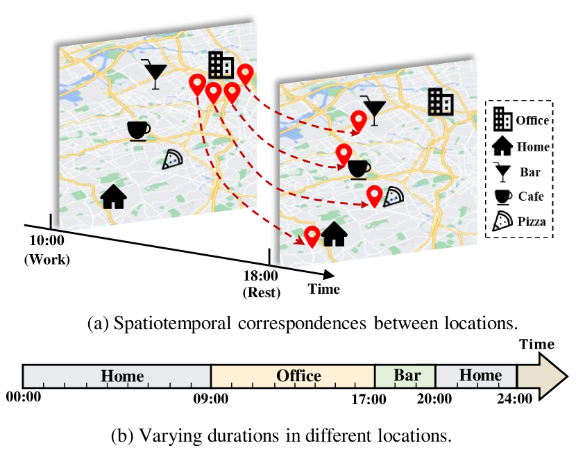
Figure 1: An illustration example. (a) depicts that various locations (HOME, Bar, Cafe, Pizza) get busy when people get off work from the office, revealing the spatiotemporal correspondences among locations. (b) depicts the successive visits of locations in an individual trajectory, resulting varying durations in different locations.

However, it is difficult to obtain human mobility trajectories recording the spatiotemporal sequences of human mobility locations due to privacy concerns and commercial limitations. The human mobility simulation task aims to generate massive artificial human mobility trajectories with high fidelity given a small set of real-world human mobility data, which can largely alleviate the scarcity and sparsity of existing data. Moreover, such controllable generations of human mobility data can perform counterfactual inference to measure the treatment effects of different strategies [8] and investigate the emergence patterns of urban growth when increasing the scales of human mobility behaviors [9, 4].

Capturing the regularities of human mobility behaviors lies at the core of human mobility simulation. Previous model-based methods [10, 11] build various conditional transition matrices of locations and maximize the log-likelihood by fitting the real-world data. Despite the simplicity and interpretability, these methods rely on large-scale mobility trajectory data and fine-grained labels of location categories, which limits their practical utility. Recently, deep learning-based methods [12, 13, 14] introduce the static relationships of locations to generate human mobility sequences in a global view. DeepMove [12] captures the sequential dependency within a single trajectory with the neural attention layer; CGE [14] obtains the global relationships of locations by the proposed static relationship matrix of locations; MoveSim [13] takes a step further to introduce the structure prior of locations with an attention layer. However, these methods focus on the static relationships of locations, while the dynamic spatiotemporal effects of locations are largely under-explored.

As shown in Figure 1, the spatiotemporal effects of locations can be observed from two aspects: the spatiotemporal correspondences and the varying durations. On the one hand, Figure 1 (a) depicts that various locations (Home, Bar, Cafe, Pizza) get busy when people get off work. It indicates the spatiotemporal correspondences between these locations, which can reflect both the spatial proximity and the functionality similarity. On the other hand, Figure 1 (b) depicts the varying durations in different locations of an illustrative trajectory, which describes the spatiotemporal continuity of human mobility behaviors. Existing methods generate the simulation trajectories without considering the varying durations, where locations with short dwell time will undoubtedly get neglected in the optimization goals.

Therefore, in this paper, we propose a novel SpatioTemporal-Augmented gRraph neural networks (STAR) to model the spatiotemporal effects of locations in a generator-discriminator paradigm. Firstly, we construct various kinds of spatiotemporal graphs to capture the spatiotemporal correspondences of locations and obtain the location embeddings with the multi-channel embedding module. Secondly, we build a dual-branch decision generator module to capture the varying durations in different locations, where the exploration branch accounts for the diverse transitions of locations and the dwell branch accounts for the staying patterns of locations. After generating a complete human trajectory iteratively, the proposed STAR is optimized by the policy gradient strategy with rewards from the policy discriminator module, playing a min-max game with the discriminator [15]. We have conducted comprehensive experiments on four real datasets for the human mobility simulation task. Results on various real-world datasets validate the superiority of our proposed STAR framework to the state-of-the-art methods. In summary, our contributions can be summarized as follows:

• We innovatively build the spatiotemporal graphs of locations to model the dynamic spatiotemporal effects among locations for the human mobility simulation task.

• A novel framework STAR is proposed to handle the spatiotemporal correspondences and the varying durations with the multi-channel embedding module and the dual-branch decision generator module, respectively.

• Extensive experiments on various real-world datasets demonstrate that the proposed STAR consistently outperforms the state-of-the-art baselines in human mobility simulation with high fidelity. The ablation studies further reveal the working mechanisms of the spatiotemporal graphs and the dwell branch.

2 Related Works

In this section, we briefly review the most-related literatures along the following lines of fields: (1) human mobility simulation and (2) graph neural networks.

2.1 Human Mobility Simulation

The human mobility simulation task aims to generate artificial mobility trajectories with realistic mobility patterns given a small set of human mobility data [16, 17, 18, 19, 13, 20]. The generated artificial trajectories must reproduce a set of spatial and temporal mobility patterns, such as the distribution of characteristic distances and the predictability of human whereabouts. Temporal patterns usually include the number and sequence of visited locations together with the time and duration of the visits, which involves balancing an individual’s routine and sporadic out-of-routine mobility patterns. And spatial patterns include the preference for short distances[1, 21], the tendency to split into returnees and explorers[22], and the fact of visiting multiple sites for constant times for individuals[23].

In the early stage, Markov-based models dominate the task of human mobility simulation. For example, First-order MC [24] defines the state as the location accessed and assumes that the next location depends only on the current location, thus constructing a transition matrix to capture the first-order transition probability among locations. HMM [25] is established with discrete emission probability and optimized by the Baum-Welch algorithm. IO-HMM [11] further extends Markov-based models by introducing more annotation information, which also improves interpretability. However, Markov-based models are limited in capturing long-term dependencies and incorporating individual preferences.

To make up the deficiency of Markov-based models, a large body of mechanistic methods have emerged, which can reproduce basic temporal, spatial, and social patterns of human mobility [19, 26, 16, 17, 18]. For example, in the Exploration and Preferential Return (EPR) model[27], an agent can select a new location that has never been visited before based on a random walk process utilizing a power-law jump-size distribution, or return to a previously visited location based on its frequency. Then several studies enhanced the EPR model by incorporating increasingly elaborate spatial or social mechanisms [22, 28, 23, 29, 30]. EPR and its extensions primarily focus on the spatial patterns of human mobility, neglecting to capture the temporal mechanisms. TimeGeo [31] and DITRAS [26] improve temporal mechanism by integrating a data-driven model into an EPR-like model to capture both routine and out-of-routine circadian preferences. Despite the interpretability of mechanistic methods, their realism is limited by the simplicity of the implemented mechanisms.

The limitations mentioned above can be addressed by deep learning generative paradigms such as recurrent neural networks (RNNs) and generative adversarial networks (GANs), which can learn the distribution of data by capturing complex and non-linear relationships in data and generate mobility trajectories from the same distribution. As a result, the deep learning approaches for human mobility simulation can generate more realistic data than traditional methods. RNN-based models prefer to maximize the prediction likelihood of the next location likelihood [32, 33], resulting in ignoring the long-term influence and the so-called exposure bias. SeqGAN [33], the pioneering work of sequence generation based on Generative Adversarial Networks (GAN) [15], proposes to optimize the generator of discrete tokens by a policy gradient technique. Based on SeqGAN, MoveSim [13] further introduces the location structure as a prior for human mobility simulation. ActSTD [34] improves the dynamic modeling of individual trajectories by the neural ordinary equation. It is worth noting that the purpose of human mobility simulation differs from that of human mobility prediction [35, 36, 37]. The former aims to produce results that reflect the characteristics of real-world data, which should not be too similar to real data so as to protect user privacy. Conversely, the latter emphasizes testing the model’s ability to recover the real data. Despite deep learning approaches proposed for human mobility prediction [38, 39], simulating daily mobility has been underexplored.

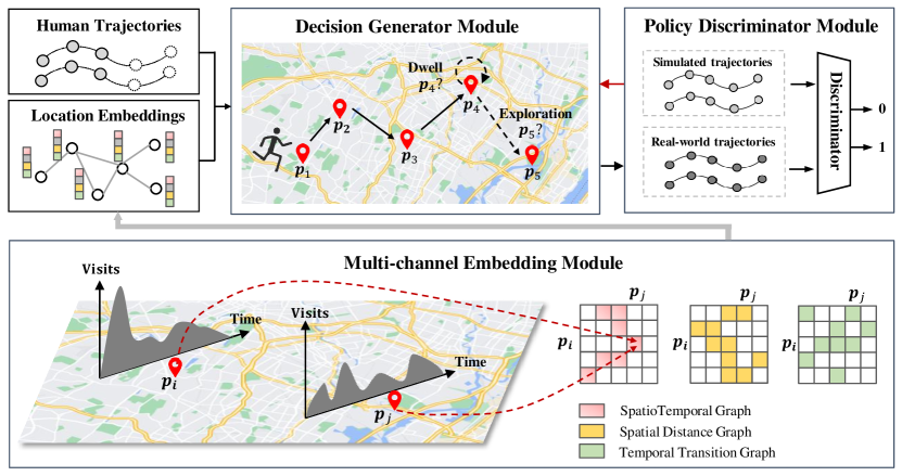
Figure 2: The overall framework of STAR. Firstly, given an observed human trajectory, the multi-channel embedding module generates location embeddings based on the proposed multi-channel spatiotemporal graphs. Secondly, the decision generator module predicts the future trajectory by balancing the exploration branch which is prone to another location and the dwell branch which decides whether to stay at the previous location. Finally, STAR is optimized in an adversarial manner by the policy discriminator module to alleviate the exposure bias of the maximum likelihood manner.

2.2 Graph Neural Networks

Recently, the rapid development of deep learning [40, 41] has inspired the researches on Graph Neural Networks (GNNs) [42, 43, 44, 45], which attracts much concern from various fields due to their widespread applications for non-grid data. Graph Convolution Networks (GCN) [43] advances the node classification task by a large margin compared to the previous methods, showing a pioneering attempt at GNNs; GraphSAGE [44] aims to perform graph learning on large-scale datasets by sampling the recursively expanded ego-graphs; Graph Attention Network (GAT) [45] weights the neighborhood importances by an adaptive attention mechanism [46]. Due to their significant progress, GNNs have been applied in various fields such as social networks, molecular structures, traffic flows, and so on.

Among the numerous fields in which GNNs are applied, urban computing is most relevant to the human mobility simulation task in this paper. Urban computing aims to understand the urban patterns and dynamics from different application domains where the big data explodes, such as transportation, environment, security, etc [47]. Due to the spatio-temporal characteristics of some typical urban data, such as traffic network flow [48, 49, 50, 51], crowd flow [52], environmental monitoring data, etc., some previous works combines graph neural networks with various temporal learning networks to capture the dynamics in the spacial and temporal dimensions [53]. The hybrid neural network architecture is collectively referred to as spatio-temporal graph neural network (STGNN).

The basic STGNN framework for predictive learning is composed of three modules: Data Processing Module (DPM) which constructs the spatio-temporal graph from raw data, Spatio-Temporal Graph Learning Module (STGLM) which extracts hidden spatio-temporal dependencies within complex social systems and Task-Aware Prediction Module (TPM) which maps the spatio-temporal hidden representation from STGLM into the space of downstream prediction tasks. As the most crucial part in STGNN, STGLM combines spatial learning networks such as spectral graph convolutional networks (Spectral GCNs), spatial graph convolutional networks (Spatial GCNs) or GATs, and temporal leaning networks such as RNNs, temporal convolutional networks (TCNs) or temporal self-attention networks (TSANs) organically through a certain spatio-temporal fusion neural architecture.

Therefore, almost all current researches focus on the design of the neural architectures in STGLM and there are many frontier methods to improve the learning of spatio-temporal dependencies. For example, THINK [54] and DMGCRN [55] perform the hyperbolic graph neural network on the Poincare ball to directly capture multi-scale spatial dependencies. ASTGCN [56] employ a typical three-branch architecture for multi-granularity temporal learning, where the data undergone the calculation of multiple GCNs and Attention networks from the three branches will be finally fused by the learnable weight matrix. STSGCN [57] fuses spatio-temporal dependencies by constructing the spatio-temporal synchronous graph. Based on STSGNN, STFGNN [58] introduces topology-based graph and similarity-based graph simultaneously to construct a spatio-temporal synchronous graph, making the spatio-temporal synchronous graph more informative. S2TAT [59] proposes a spatio-temporal synchronous transformer framework to enhance the learning capability with attention mechanisms.

However, there are two main differences between our work and the existing researches on STGNN. First, in previous studies, the topological structure of the spatio-temporal graph (e.g. road network) is fixed, while ours is self-constructed and closely related to the order of the locations visited by individuals. Second, the existing methods based on STGNN are almost used for predictive learning tasks in urban computing, but our approach focuses on simulation task which emphasizes the effective capture of the overall patterns rather than the accurate prediction of a single entity.

3 Problem Statement

A human mobility trajectory can be defined as a spatiotemporal sequence $s=[\tau_{1},\tau_{2},\cdots,\tau_{L}]$. The $l$-th visit record $\tau_{l}$ represents a tuple $(p_{l},t_{l})$, where $p_{l}$ records the location ID and $t_{l}$ records the visit timestamp. The human mobility simulation problem is thus defined as follows.

DEFINITION 1. (Human Mobility Simulation). Given a real-world mobility trajectory dataset $\mathcal{S}=\{s_{1},s_{2},\cdots,s_{m}\}$, our goal is learning to simulate human mobility behaviors in order to generate an artificial trajectory $\hat{s}=\left[\hat{\tau}_{1},\hat{\tau}_{2},\dots,\hat{\tau}_{L}\right]$ with fidelity and utility.

Directly maximizing the likelihood of the sequence generation model would undoubtedly cause the eposure bias [32, 33] towards the training data, resulting in poor generalization abilities. Therefore, it is useful to advance the human mobility simulation under the framework of SeqGAN [15, 33], which coordinates the optimization of the generator (sequence generation model) and a discriminator in a min-max game, written as

$$\min_{\mathbf{\theta}}\max_{\mathbf{\phi}}\mathbb{E}_{\mathbf{x}\sim\pi}{\left[\log D_{\mathbf{\phi}}(\mathbf{x})\right]}+\mathbb{E}_{\mathbf{x}\sim\pi_{d}}\left[\log\left(1-D_{\mathbf{\phi}}(\mathbf{x})\right)\right],$$ (1)

where $\mathbf{x}$ is the sampled mobility trajectory, $\mathbb{E}_{\pi}$ represents the expected reward of the sequences under the policy $\pi$, and $\mathbb{\pi}_{d}$ samples $\mathbf{x}$ from the ground-truth trajectory data $\mathcal{S}$.

4 Methods

The proposed SpatioTemporal-Augmented gRaph neural networks (STAR) aims to capture the spatiotemporal correspondences among locations and the varying durations in different locations to advance the human mobility simulation task in a spatiotemporal way. As illustrated in Figure 2, the STAR framework consists of three key components: (i) the multi-channel embedding module learns spatiotemporal semantics of locations by the dense representations based on the proposed multi-channel location graphs with the partial observed human trajectories; (ii) the decision generator module tackles the varying duration problem by the exploration branch and the dwell branch, alleviating the effects of highly repetitive patterns in mobility trajectories; (iii) the policy discriminator module provides the rewards for the generator at each step based on the policy gradient technique.

4.1 Multi-channel Embedding Module

4.1.1 Location Graphs

Let $\mathcal{P}=\{p_{0},p_{1},\cdots,p_{N}\}$ be the set of locations. The spatiotemporal correspondences among locations $p_{i},p_{j}\in\mathcal{P}$ can be well modeled by their correspondence scores $\epsilon(p_{i},p_{j})$ with a correspondence function $\epsilon(\cdot,\cdot)$, resulting in a location-location adjacency graph $G=(\mathcal{P},\mathcal{E})$. The edge set $\mathcal{E}$ of the graph contains pairwise correspondences of locations. For example, if the function $\epsilon(\cdot,\cdot)$ measures the geographical proximity of locations, the constructed graph $G$ represents a $K$-nearest neighbor spatial graph of all locations. Based on the spatial graph, our model will generate human mobility trajectories in consideration of geographical effects.

Therefore, to go beyond the geographical effects, we firstly build a Spatial Distance Graph (SDG) and Temporal Transition Graph (TTG) based on the observed human mobility trajectories, which are constructed from the spatial and temporal perspectives, respectively. Secondly, we propose a SpatioTemporal Graph (STG) by measuring the Wasserstein distance [60] of location visit distributions to capture the spatiotemporal effects, which combines the spatial and temporal dynamics of locations simultaneously.

Spatial Distance Graph. The proposed SDG is constructed based on the spatial proximity of a location pair $(p_{i},p_{j})$, which indicates the spatial cooperation effects in human trajectories. Let $w_{ij}$ be the spatial proximity score of $\epsilon(p_{i},p_{j})$, we have to build the Spatial Distance Graph (SDG) out of the Cartesian score set of $\mathcal{P}\times\mathcal{P}$, written as

$$G_{\mathrm{SDG}}=\begin{cases}w_{ij},&w_{ij}\in\text{top}_{k}(\epsilon(p_{i},\cdot)),\\ 0,&\text{Otherwise},\end{cases}$$ (2)

which remains the top-$k$ neighbors from all locations. The spatial proximity function is usually implemented by Euclidean distance for simplicity.

Temporal Transition Graph. The SDG can reveal the spatial proximity of locations, but ignores the mobility patterns of human trajectories. We further propose the Temporal Transition Graph (TTG) to encode the mobility patterns based on the partial observed human trajectories. Let $s=[\cdots,\tau_{l},\tau_{l+1},\cdots]$ be a human trajectory and $\tau_{l}=(p_{i},t_{l}),\tau_{l+1}=(p_{j},t_{l+1})$. We record the proximity score between $p_{i}$ and $p_{j}$ as $\epsilon(p_{i},p_{j})=1$ and obtain the summed scores by $w_{ij}=\sum_{(pi,p_{j})\in\mathcal{S}}\epsilon(p_{i},p_{j})$. The graph is thus formulated as

$$G_{\mathrm{TTG}}=\begin{cases}w_{ij},&w_{ij}>0,\\ 0,&\text{Otherwise}.\end{cases}$$ (3)

The obtained TTG can detailedly describe the mobility patterns from the temporal transition perspective.

SptioTemporal Graph. The SDG and TTG describe the location relationships from the spatial and temporal perspectives, respectively, thus ignore the other aspect to some extent. We further characterize the location functionality with a SpatioTemporal Graph (STG) by its visit distribution over time, which can describe the spatial proximity with the spatial cooperation effects and the temporal proximity with the visit distribution similarity. For instance, cafes often open from morning to evening, while bars keep open till midnight. The visit distribution $F_{p_{i}}$ of a location $p_{i}$ is calculating its normalized visit counts in the observed records $\mathcal{S}_{p_{i}}$ by discretizing the timestamps into $T$ time slots: $F_{p_{i}}(t)=\frac{1}{|\mathcal{S}_{p_{i}}|}\sum_{t_{k}\in\mathcal{S}_{p_{i}}}\mathbbm{1}{[t_{k}=t]}$. The obtained visit distribution $F_{i}$ can well describe the location from both the spatial and the temporal aspects. On the one hand, neighborhood locations often share similar visit distributions based on geographical effects, which have been widely adopted in Location-based Services. On the other hand, locations far apart can also share similar visit distributions since they provide peer functionalities like eating or drinking. Thus, the Wasserstein distance [60] is employed here to measure the distances of the visit distributions $F_{\mathcal{P}}$ of locations to differentiate their individual functionalities, defined as follows:

$$\begin{gathered}d(p_{i},p_{j})=\inf_{\pi\in\prod[F_{p_{i}},F_{p_{j}}]}\int_{x}\int_{y}\pi(x,y)|x-y|\mathrm{d}x\mathrm{d}y,\\ \text{ s.t. }\int\pi(x,y)\mathrm{d}y=F_{p_{i}}(x),\int\pi(x,y)\mathrm{d}x=F_{p_{j}}(y),\end{gathered}$$ (4)

where $\pi(x,y)$ is a joint distribution of $F_{p_{i}}$ and $F_{p_{j}}$. The proximity score can be simply defined as $\epsilon(p_{i},p_{j})=1-d(p_{i},p_{j})\in[0,1]$. Let $w_{ij}=\epsilon(p_{i},p_{J})$, the graph can be formulated as

$$G_{\mathrm{STG}}=\begin{cases}w_{ij},&w_{ij}\in\text{top}_{k}(\epsilon(p_{i},\cdot)),\\ 0,&\text{Otherwise}.\end{cases}$$ (5)

The proposed STG can capture the spatiotemporal dynamics of locations in a distribution way.

Overall, the above multi-channel location graphs are denoted by $\mathcal{G}=\{G_{\mathrm{SDG}},G_{\mathrm{TTG}},G_{\mathrm{STG}}\}$. The connection edges of a location pair $(p_{i},p_{j})\in G$ are naturally weighted with their proximity scores, indicating the spatiotemporal correspondences given by different measurements. However, these scores are not aligned with the human mobility simulation task, which can cause the inconsistent problems between the spatiotemporal graphs and the simulation task. To bridge the gap between the graphs and the task, we alternatively propose a Vanilla version based on the Weighted version, written as

$$\begin{split}\hat{\epsilon}(p_{i},p_{j})=\begin{cases}1,&(p_{i},p_{j})\in G,\\ 0,&\text{Otherwise}.\\ \end{cases}\end{split}$$ (6)

The Vanilla graph regards all neighbors as the same, benefiting for the model optimization without the computed weights of the multi-channel graphs.

4.1.2 Location Embeddings

After establishing the above graphs, location embeddings can be obtained by the following procedure.

Firstly, we implement the features of the location set $\mathcal{P}$ at the input layer by a learnable embedding matrix with end-to-end optimization, following the common training paradigm of human mobility simulation. Secondly, to adaptively aggregate the useful information in terms of the graph heterogeneity, we adopt the attention layer of graphs [45] to perform multi-channel attention over all kinds of spatiotemporal graphs, namely $\mathcal{G}=\{G_{\mathrm{SDG}},G_{\mathrm{TTG}},G_{\mathrm{STG}}\}$. Given location embeddings $\mathbf{H}^{l-1}_{G}$ from the previous $l-1$-th layer (initialized embeddings at the input layer), our spatiotemporal attention layer computes the node embeddings in a multi-head manner by

$$\mathbf{h}^{l}_{i}=\Big{\|}_{k=1}^{K}{\text{ReLU}}\left(\sum_{j\in\mathcal{N}_{i}}\alpha^{k}_{ij}W^{k}\mathbf{h}_{j}^{l-1}\right),$$ (7)

where $\alpha_{ij}^{k}$ is the $k$-th attention scores of the edge $(p_{i},p_{j})$, $\mathcal{N}_{i}$ provides the neighbors of location $p_{i}$, $K$ is the number of attention heads, $\|$ is the concatenation operation, $W^{k}$ is the transformation matrix of $k$-th attention head, and ReLU is a non-linear activation function.

For simplicity, the $l$-th layer location embeddings are summed over all graphs: $\mathbf{H}^{l}=\sum_{G\in\mathcal{G}}\mathbf{H}^{l}_{G}$. The final location embeddings are denoted by $\mathbf{H}_{\mathcal{P}}$.

4.2 Decision Generator Module

The multi-channel embedding module provides location embeddings via our dedicated spatiotemporal graphs, enhancing the representation quality used in the following decision generator module. The decision generator module predicts the next location based on the observed partial mobility trajectory, which is also generated by the decision generator sequentially. Besides the common exploration branch of GANs, we further propose the dwell branch to cope with the varying durations of locations as shown in Figure 1 (b), which also reduces the optimization difficulty to some extent. Since the policy discriminator will not give classification results until the trajectory sequence is finished, we adopt the Monte-Carlo strategy to iteratively predict the next location until the required length.

4.2.1 Exploration Branch

Suppose that a partial mobility trajectory $s_{1:l}=\{(p_{1},t_{1}),(p_{2},t_{2}),\cdots,(p_{l},t_{l})\}$ is observed, the exploration branch aims to predict the next location $\hat{p}_{l+1}$ that maximizes the decision reward given by the policy discriminator module, where $t_{l+1}$ is assumed uniformly spaced with $t_{l}$ for simplicity. Given a bunch of location embeddings $\mathbf{H}_{\mathcal{P}}$ from the multi-channel embedding module, we firstly fetch the corresponding input embeddings of the trajectory, denoted by $\mathbf{h}_{s}=\{\mathbf{h}_{p_{0}},\mathbf{h}_{p_{1}},\cdots,\mathbf{h}_{p_{l}}\}$. To facilitate the sequence modeling and training efficiency, we adopt the Gated Recurrent Unit [61] as our sequence model, written as

$$\mathbf{h}_{l},z_{l}=\mathrm{GRU}(\mathbf{h}_{p_{l}},z_{l-1}),$$ (8)

where the hidden state $z_{l-1}$ is initialized as zero vectors in the first step. The obtained sequence representation $\mathbf{h}_{l}$ is fed into a linear layer to predict the probability of the next locations by

$$\hat{p}_{l+1}=\mathrm{softmax}(\mathbf{h}_{l}\times\mathbf{W}_{p}+\mathbf{b}_{p}).$$ (9)

Then the outputs of the exploration branch $\hat{p}_{l+1}$ together with the outputs of the dwell branch determine the next location iteratively until the sequence is finished.

4.2.2 Dwell Branch

Motivated by the varying durations of locations in mobility trajectories, we specially design a dwell branch to predict the probability of staying at the previous location, which can inform the model to dwell or explore. Intuitively, the duration of a specific location is determined by the spatiotemporal context, and the cumulative duration of the trajectory, where the former can be well captured by the exploration branch and the latter lacks specific modeling. For a highly repetitive trajectory dataset, the optimization goal will be overwhelmed by the repetitive locations, leading to the ignorance of diverse behaviors. Therefore, it is necessary to build the dwell branch to predict whether to stay at the previous location to alleviate the learning difficulties of the exploration branch. Taking the sequence representation $\mathbf{h}_{l}$ for the dwell branch classification is straightforward. However, it ignores the saturability of human mobility behaviors [1] that the durations of locations are usually upper-bounded to some extent. We thus combine the sigmoid function with an exponentially decaying coefficient to reduce the effects of a long-duration location, written as

$$\hat{y}_{l+1}^{d}=\mathrm{sigmoid}(\mathbf{h}_{l}\mathbf{W}_{d}+\mathbf{b}_{d})\cdot\exp(-{\beta}\cdot\mathrm{C}(s_{1:l},p_{l})),$$ (10)

where the hyper-parameter $\beta$ adjusts the decaying rate and $\mathrm{C}(s_{1:l},p_{l})=\sum_{p_{k}\in s_{1:l}}\mathbbm{1}[p_{k}=p_{l}]$ counts the frequency of $p_{l}$ in the observed trajectory. $\beta$ is set to 1 by default.

Finally, the decision generator module balances the location predictions $\hat{p}_{l+1}$ of the exploration branch and the dwell predictions $\hat{y}_{l+1}^{d}$ by sampling from the output distributions, written as

$$\begin{split}p_{l+1}=\begin{cases}p_{l},&l>1\;\text{and}\;\Psi(\hat{y}^{d}_{l+1})=1,\\ \Psi(\hat{p}_{l+1}),&\text{Otherwise},\\ \end{cases}\end{split}$$ (11)

where $\Psi(.)$ samples a location by polynomial sampling from a given probability distribution.

4.3 Policy Discriminator Module

As discussed in [32, 33], maximizing the likelihood of sequence models would suffer from the exposure bias of the training data, thus generalizing poorly to the testing data. Recently, variants of GANs [33, 13] have shown their successful applications in sequence generation tasks by back-propagating the policy gradients into the generator. Therefore, we follow the generator-discriminator paradigm to perform human mobility simulation in an adversarial manner.

By generating and sampling iteratively in the decision generator module, a set of generated trajectories $\mathcal{T}_{G}$ are fed into the policy discriminator module $D_{\phi}$. Since a powerful discriminator might hinder the optimization of the generator $G_{\theta}$, we build a simple yet efficient discriminator $D_{\phi}$ that contains an embedding matrix of locations and classifies the trajectory sequence as real data or fake data based on a GRU layer, written as

$$\mathcal{L}_{D}=\mathbb{E}_{\mathbf{x}\in\mathcal{T}_{R}}\log D_{\phi}(\mathbf{x})+\mathbb{E}_{(\mathbf{x})\in\mathcal{T}_{G}}\log\left(1-D_{\phi}(\mathbf{x})\right),$$ (12)

where $\mathcal{T}_{R}$ and $\mathcal{T}_{G}$ are real and generated trajectories, respectively. The step-by-step predictions of the decision generator module $G_{\theta}$ receives the policy gradients from the discriminator $D_{\phi}$ by unfolding the classification reward recursively following the REINFORCE algorithm [62], written as

$$\nabla_{\theta}=\nabla_{\theta}\mathbb{E}_{P_{\theta}(\mathbf{x})}[R(\mathbf{x})]=\mathbb{E}_{P_{\theta}(\mathbf{x})}\left[R(\mathbf{x})\nabla_{\theta}\log P_{\theta}(\mathbf{x})\right],$$ (13)

where $P_{\theta}$ denotes the generated distribution by the decision generator $G_{\theta}$, $\mathbf{x}$ is the generated mobility trajectory, and the reward $R(\mathbf{x})$ is the classification loss from the discriminator $D_{\phi}$. The generator $G_{\theta}$ can be optimized in this way.

5 Experiment

In this section, we conduct experiments for the human mobility simulation task on four real-world datasets to evaluate the performance of our proposed STAR framework. We first briefly introduce the four datasets, baseline methods, and evaluation metrics. Then, we compare STAR with the state-of-the-art baselines for the human mobility simulation task and present the experiment results. Furthermore, we analyze the impact of different modules and hyperparameters on model performance. Finally, we present the geographical visualization results of our proposed STAR method and the baseline methods.

We aim to answer the following key research questions:

• RQ1: How does STAR perform compared with other state-of-the-art methods for the human mobility simulation task?

• RQ2: How do different modules (different kinds of spatiotemporal graphs and the dwell branch) affect STAR?

• RQ3: How do hyper-parameter settings (the depth of layer and the number of attention heads) influence the performance of STAR?

• RQ4: How do we qualitatively assess the quality of human trajectories simulated by different methods with regard to the real trajectories?

TABLE I: The statistics of four datasets.

Dataset	Timespan	$|$Users$|$	$|$Locations$|$	$|$Visits$|$
NYC	Apr. 2012 - Feb. 2013	1,083	38,333	227,428
TKY	Apr. 2012 - Feb. 2013	2,293	61,858	573,703
Moscow	Apr. 2012 - Sep. 2013	10,464	88,036	806,196
Singapore	Apr. 2012 - Sep. 2013	8,784	45,525	397,873

TABLE II: Performance of the proposed STAR framework and baselines in terms of JSD for human mobility trajectory simulation. A lower JSD value indicates a better performance. Bold and underline means the best and the second-best results.

	NYC						TKY
Metrics(JSD)	Distance	Radius	Duration	DailyLoc	G-rank	I-rank	Distance	Radius	Duration	DailyLoc	G-rank	I-rank
Markov[10]	0.1256	$\underline{0.3742}$	0.0037	0.2667	0.1119	0.0668	0.1379	0.4246	0.0077	0.2615	0.0413	0.0659
IOHMM[11]	0.4179	0.6022	0.0046	0.1071	0.6931	0.0750	0.3368	0.5438	0.0059	0.1732	0.6931	0.0577
LSTM[63]	$\underline{0.1239}$	0.3862	0.0014	$\underline{0.0776}$	$\underline{0.0772}$	0.0728	0.1334	0.4479	0.0019	$\underline{0.0415}$	0.0350	0.0615
DeepMove[12]	0.4068	0.5851	0.0064	0.3139	0.4030	0.0593	0.3349	0.5374	$\underline{0.0010}$	0.0478	0.2926	0.0534
GAN[15]	0.4405	0.6298	0.0026	0.0839	0.2418	0.0364	0.3644	0.5653	0.0046	0.1881	0.1599	0.0557
SeqGAN[33]	0.1774	0.4374	0.0043	0.0803	0.1159	0.0528	$\underline{0.1260}$	$\underline{0.4193}$	0.0011	0.0452	$\underline{0.0267}$	0.0591
MoveSim[13]	0.4571	0.5977	0.0013	0.0885	0.2474	0.0624	0.3459	0.5511	0.0036	0.1655	0.0777	$\underline{0.0476}$
CGE[14]	0.4154	0.6338	0.1101	0.3925	0.3172	$\underline{0.0476}$	0.4151	0.5816	0.0041	0.1792	0.1820	0.0457
STAR (Ours)	0.1105	0.3636	$\underline{0.0011}$	0.0580	0.0359	0.0624	0.1196	0.4178	0.0005	0.0402	0.0259	0.0693
	Moscow						Singapore
Metrics(JSD)	Distance	Radius	Duration	DailyLoc	G-rank	I-rank	Distance	Radius	Duration	DailyLoc	G-rank	I-rank
Markov[10]	$\underline{0.0083}$	0.0555	0.0136	0.1729	0.1229	0.0694	0.0078	0.0409	0.0060	0.1427	0.2505	0.0797
IOHMM[11]	0.1050	0.0610	0.0137	0.2832	0.1639	0.0733	0.0447	0.0456	0.0053	0.1729	0.1839	0.0693
LSTM[63]	0.0127	0.0208	0.0192	0.4412	0.3621	0.0626	$\underline{0.0066}$	$\underline{0.0097}$	0.0777	0.6457	0.2965	0.0596
DeepMove[12]	0.1098	0.0528	0.0046	0.1592	0.3814	0.0532	0.0365	0.0279	0.0018	$\underline{0.0405}$	0.2931	$\underline{0.0459}$
GAN[15]	0.1073	0.0735	0.0098	0.2511	0.2158	0.0755	0.0494	0.0438	0.0042	0.1608	0.3325	0.0577
SeqGAN[33]	0.0123	0.0207	$\underline{0.0036}$	0.0434	$\underline{0.0307}$	0.0659	0.0106	0.0106	0.0028	0.0696	$\underline{0.0294}$	0.0451
MoveSim[13]	0.0235	$\underline{0.0179}$	0.0457	0.4915	0.1252	$\underline{0.0523}$	0.0096	0.0099	$\underline{0.0016}$	0.5643	0.2459	0.0487
CGE[14]	0.0328	0.6931	0.0062	0.2322	0.2170	0.0659	0.1798	0.1008	0.0785	0.5164	0.3254	0.0581
STAR (Ours)	0.0049	0.0152	0.0023	$\underline{0.0497}$	0.0294	0.0485	0.0062	0.0095	0.0014	0.0371	0.0287	0.0485

5.1 Datasets

To ensure reproducibility and facilitate fair comparisons with previous works, we evaluates the human mobility of four cities (i.e., New York, Tokyo, Moscow and Singapore) extracted from the publicly available dataset Foursquare in line with previous studies [14, 64]. The timespan and the numbers of users, locations and visit records in each dataset are shown in Table I. The wide range of the timespan and the large-scale visits can sufficiently compare the STAR framework against baseline methods. In experiments, we use the original raw datasets that only contain the GPS coordinates of each location and user check-in records, and pre-process them following the protocol of the human mobility simulation task.

Specifically, we split the whole dataset into three parts: a training set for training the generative model, a validation set for finding the best parameters of models and a testing set for the final evaluation of various metrics. The partition of the four datasets is all set as 7:1:2. Besides, we set the basic time slot as an hour of the day for the convenience and universality of modeling. Finally, in order to ensure the effectiveness and accuracy of modeling, we only remain the trajectories with visit records greater than eight each day.

5.2 Baseline Methods and Evaluation Metrics

We compare the performance of the STAR framework with the following state-of-the-art baseline methods.

• Markov [10] is a well-known probability method describing the state transitions, which treats the locations as states and calculates the transition probability of locations.

• IO-HMM [11] fits the probability model with annotated user activities as its latent states and then generates human trajectories based on the hidden Markov model.

• LSTM [63] improves the classical RNN by the dedicated memory cell and the forget gate to enhance the long-term dependency modeling.

• DeepMove [12] learns the periodic patterns of mobility by the recurrent network and the neural attention layer.

• GAN [15] uses two LSTMs as the generator and the discriminator in our settings, respectively.

• SeqGAN [33] solves the discrete sequence generation problem based on the policy gradient technique with GAN, which is suitable for trajectory generation.

• MoveSim [13] simulates mobility trajectory by augmenting the prior knowledge of the generator and regularizing the periodicity of sequences.

• CGE [14] generates location sequences based on a newly constructed static graph from historical visit records.

Following the common practice in previous works [13, 65], we adopt six metrics to evaluate the quality of generated data by comparing the distributions of important mobility patterns between the simulated trajectories and the real trajectories from different perspectives.

• Distance: The moving distance among locations in individuals’ trajectories is a metric from the spatial perspective.

• Radius: Radius of gyration is the root mean square distance of all locations from the central one, which represents the spatial range of individual daily movement.

• Duration: Dwell duration among locations in mobility trajectories is a metric from the temporal perspective.

• DailyLoc: Daily visited locations are calculated as the number of visited locations per day for each user.

• G-rank: The number of visits per location is calculated as the visiting frequency of the top-100 locations.

• I-rank: It is an individual version of G-rank.

Specifically, we use Jensen-Shannon divergence (JSD) [66] to measure the discrepancy of the distributions between the generated data and real-world data. The JSD metric is defined as follows:

$$\operatorname{JSD}(p\|q)=H((p+q)/2)-\frac{1}{2}(H(p)+H(q))$$ (14)

where $p$ and $q$ are two distributions for comparison, and $H$ is the Shannon entropy. A lower JSD denotes a closer match to the statistical characteristics and thus indicates a better generation result.

5.3 Experimental Settings

For a fair comparison, we set all methods with the following settings: the hidden dimension of embeddings is set to 32, the number of epochs is set to 50, and the batch size is set to 32. Other specific hyper-parameters of these baselines follow the best settings in their papers. The proposed STAR framework is implemented in PyTorch [67]. In default settings, the learning rate is set to 0.01 and the dropout ratio is set to 0.6. The number of attention layers is searched over {1, 2}, and the number of attention heads is searched over {1, 2, 4}.

5.4 RQ1: Performance Comparison

Table II presents the performance in retaining the data fidelity of our framework and the eight competitive baselines on four real-world datasets at different scales. The results reveal the following discoveries:

• Our framework steadily achieves the best performance. STAR achieves the best performance on all datasets with ranking first on nineteen metrics and ranking second on two metrics over twenty four metrics of the four datasets. For the nineteen ranking first metrics, compared with the best baseline, our method reduces the JSD up to 53.50%. For the other five metrics, namely Duration on the NYC dataset, DailyLoc on the Moscow dataset, I-rank on the NYC, TKY and Singapore dataset, our framework also obtains competitive performance with the best baseline.

• Model-based methods are limited in simulating human mobility. Markov performs worse on the time-dependent metrics (i.e., duration and dailyloc) but better on the distance-based metrics (i.e., Distance and Radius), because it obtains the next location based on the distribution of historical transition probabilities, which is in line with our intuition that individuals are prone to the near areas. The performance of IO-HMM is also unsatisfactory, because its modeling relies on extensive manual labeling, which places higher demands on the quality of data. For example, lack of records at home interferes with the annotation of Home label, which degrades the predictive performance of IO-HMM. In addition, the sparsity of data introduces errors in the labeling of dwell time.

• Deep learning methods for mobility prediction task perform poorly on hunam mobility simulation task. LSTM and DeepMove are all trained with the short-term goal (i.e. next location prediction) and thus do not perform particularly well on the human mobility simulation task. Unlike human mobility simulation, which emphasizes producing results that reflect various mobility patterns in real trajectories, human mobility prediction highlights the recovery of the next location in real-data and lacks the learning of the global patterns.

• Generative networks fail to generate realistic human trajectories without trajectory pre-training. GAN performs the worst across almost all metrics, indicating that it is difficult to capture the hidden patterns of human mobility when learning with noisy and inaccurate raw data. SeqGAN is pre-trained by the task based on human mobility modeling, so it yields much better results than GAN.

• It is essential to model dynamic spatiotemporal dependencies among locations. Although CGE leverages graph structure for data augmentation, its graph is static and the node embeddings generated by Word2vec cannot be learned and updated in the process of mobility simulation, so it only learns better on several metrics but performs poorly overall. MoveSim introduces the urban structure modeling component especially for locations, so it achieves the best result on Duration metric of the NYC dataset and the second-best result on I-rank metric of the TKY and Moscow dataset, radius metric of the Moscow dataset and Duration metric of the Singapore dataset.

5.5 RQ2: Ablation Study of STAR

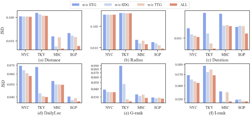
Figure 3: Ablation study on the channels of graphs. STG, SDG and TTG represent SpatioTemporal Graph, Spatial Distance Graph and Temporal Transition Graph respectively. MSC and SGP are short for Moscow and Singapore. A lower JSD value indicates a better performance.

TABLE III: Ablation study on edge type of GNNs in STAR in terms of JSD. MSC and SGP are short for Moscow and Singapore. A lower JSD value indicates a better performance.

Dataset	Method	Distance	Radius	Duration	DailyLoc	G-rank	I-rank
NYC	Weighted	0.1117	0.3665	0.0013	0.0613	0.0383	0.0628
	Vanilla	0.1105	0.3636	0.0011	0.0580	0.0359	0.0624
	% Improv.	1.07%	0.79%	15.38%	5.38%	6.27%	0.64%
TKY	Weighted	0.1247	0.4220	0.0006	0.0438	0.0298	0.0697
	Vanilla	0.1196	0.4178	0.0005	0.0402	0.0259	0.0693
	% Improv.	4.09%	1.00%	16.67%	8.22%	13.09%	0.57%
MSC	Weighted	0.0081	0.0201	0.0029	0.0501	0.0335	0.0720
	Vanilla	0.0049	0.0152	0.0023	0.0497	0.0294	0.0485
	% Improv.	39.51%	24.38%	20.69%	0.80%	12.24%	32.64%
SGP	Weighted	0.0098	0.0115	0.0012	0.0384	0.0295	0.0494
	Vanilla	0.0062	0.0095	0.0014	0.0371	0.0287	0.0485
	% Improv.	36.73%	17.39%	-16.67%	3.39%	2.71%	1.82%

TABLE IV: Ablation study on dwell branch in STAR in terms of JSD. DB, MSC and SGP are short for the dwell branch, Moscow and Singapore. A lower JSD value indicates a better performance.

Dataset	Method	Distance	Radius	Duration	DailyLoc	G-rank	I-rank
NYC	w/o DB	0.1152	0.3717	0.0013	0.0582	0.0376	0.0659
	STAR	0.1105	0.3636	0.0011	0.0580	0.0359	0.0624
	% Improv.	4.08%	2.18%	15.38%	0.34%	4.52%	5.31%
TKY	w/o DB	0.1237	0.4293	0.0004	0.0433	0.0343	0.0705
	STAR	0.1196	0.4178	0.0005	0.0402	0.0259	0.0693
	% Improv.	3.31%	2.68%	-25.00%	7.16%	24.49%	1.70%
MSC	w/o DB	0.0076	0.0180	0.0027	0.0501	0.0297	0.0555
	STAR	0.0049	0.0152	0.0023	0.0497	0.0294	0.0485
	% Improv.	35.53%	15.56%	14.81%	0.80%	1.01%	12.61%
SGP	w/o DB	0.0065	0.0101	0.0016	0.0384	0.0320	0.0497
	STAR	0.0062	0.0095	0.0014	0.0371	0.0287	0.0485
	% Improv.	4.62%	5.94%	12.50%	3.39%	10.31%	2.41%

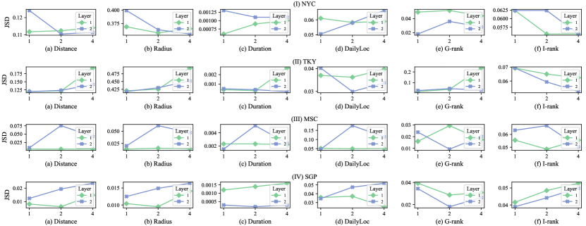
Figure 4: Effects of the number of layers and attention heads in STAR.

In this part, we attempt to investigate the effectiveness of different modules in the STAR framework.

5.5.1 Designs of Multi-channel Graph

In order to learn the spatiotemporal correspondence among locations, we design three kinds of spatiotemporal graphs in the multi-channel embedding module to represent the node embeddings separately and obtain the final embeddings with a fusion layer. To verify the effectiveness of the three graphs in STAR, we get rid of any of them (i.e., without SpatioTemporal Graph, without Spatial Distance Graph and without Temporal Transition Graph) to learn the node embeddings and perform human mobility simulation. The comparison of their simulated results is shown in Figure 3.

Compared with the results predicted by removing any of the three graphs, the fused embedding achieves optimal performance on almost all metrics over the four datasets. In addition, the average performance of removing SpatioTemporal Graph is the worst on six metrics, especially on Distance, Duration, DailyLoc and G-rank metric, which measure the effectiveness of simulated trajectories from both spatial and temporal perspectives. It indicates that only relying on the static distance and transition information of locations is not enough to carry out accurate trajectory simulation.

Eliminating the Spatial Distance Graph results in a decline of performance on distance-based metrics (i.e. Distance and Radius), which is as per our hypothesis. However, it scores well on preference-based metrics (i.e. G-rank and I-rank), which is attributed to the SpatioTemporal Graph and Temporal Transition Graph effectively learning frequently visited locations in the trajectories. Furthermore, removing the Temporal Transition Graph results in inferior performance compared to remaining all three graphs but surpasses removing any other graph overall, which suggests that the SpatioTemporal Graph can aptly supplement the temporal transition information of trajectories.

5.5.2 Designs of Edge Type in GNNs

In order to explore the effect of edge weight in GNNs on model performance, we set two edge types for model, Weighted and Vanilla. Weighted retains the weights of edges in the three graphs, that is, the three graphs before binaryzation, while Vanilla only uses the adjacency relationship of the three graphs to learn node embedding. We list their performance in Table III.

It can be seen from the results that Vanilla is better than Weighted on almost all metrics of the four datasets, especially on the Distance metric of the Moscow and Singapore dataset, the improvement reaches 39.51% and 36.73%, respectively. The reasons for the result may be as follows. Firstly, Vanilla are simpler to implement, while Weighted increases the training time and degrades the performance. Secondly, Weighted edges may assign significant weights to noisy or irrelevant features, leading to reduced model performance. In contrast, Vanilla only consider the presence or absence of an edge, which can be more resilient to noise.

The six metrics can be classified into three categories based on the level of improvement they show when comparing the Vanilla graph to the Weighted graph. Distance-based metrics (i.e. Distance and Radius) exhibit the highest improvement, whereas time-dependent metrics (i.e. duration and dailyloc) show the least improvement. Preference-based metrics (i.e. G-rank and I-rank) show moderate improvements. The underlying reason lies in the fact that our proposed multi-channel graphs explicitly encode the distance and user preferences of locations, while lack the time-dependent constraints. Additionally, the long-tailed distribution of the Weighted version might exaggerate the uneven distribution of location frequencies.

5.5.3 Designs of Dwell Branch

The dwell branch which allows individuals to remain in the current location with a learnable probability, aims to adaptively perceive the varying durations in mobility trajectories. We conduct ablation experiments on this component to verify its effectiveness, and the results are shown in Table IV.

As we can observe, the design of the dwell branch enhances the performance on twenty three metrics over twenty four metrics of the four datasets, with the most significant improvement observed with the Distance metric on the Moscow dataset, which is up to 35.53%. It implies that enabling individuals to dwell in a specific location with a learnable probability can facilitate a more comprehensive representation of complex real-world behavior, consequently improving the performance of various metrics from different perspectives.

Specifically, there are two reasons for the performance improvement. First of all, staying at the current location with a certain probability reduces the likelihood of long-distance movement for a individual. As a result, the dwell branch facilitates the acquisition of distance-related patterns and features, subsequently improving the performance of distance-based and time-dependent metrics. Secondly, individuals tend to visit several specific locations frequently and thereby the learnable stay probability can increase individuals’ visit probability at frequently visited places, which effectively captures the mobility preferences of real trajectories from both collective and individual view.

It is worth noting that the dwell branch achieves the most significant performance improvement on the Moscow dataset, as expected. Due to the high frequency of staying in the previous location in the Moscow dataset, the learnable stay probability is essential for modelling repeated movement patterns within the trajectories more effectively.

5.6 RQ3: Parameter Sensitivity of STAR

Parameter sensitivity analysis can help us understand how changes in parameters of model affect its performance, which is conducive to optimizing the model for better performance, identifying key parameters that have the most important impact on results, and assessing the reliability and robustness of the model. Figure 4 demonstrates the parameter sensitivity of STAR on two key hyper-parameters, the number of GAT layers and attention heads, which affect the graph convolution architecture in the STAR framework.

We plot the grid search results of the number of GAT layers over {1, 2} and the number of attention heads over {1, 2, 4} to thoroughly test the STAR framework on twenty four metrics over the four datasets. As can be seen from Figure 4, the performance of STAR is robust under different hyperparameter settings, which indicates different hyperparameter values wouldn’t affect its superiority over other baselines.

Specifically, the performance of different hyperparameters varies from metric to metric. On distance-based metrics (i.e., Distance and Radius), only a simple model with a few number of GAT layers and attention heads can achieve good performance. As the number of layers and attention heads increases, the performance of the model on distance-based metrics deteriorates due to overfitting. The phenomenon emerges since moving distance is the most conspicuous pattern of trajectories, where the distance-related features in trajectories can be effectively modeled with fewer GAT layers and attention heads. On time-dependent metrics (i.e., duration and dailyloc), the performance of the model exhibits minimal fluctuations with the changes in the number of GAT layers and attention heads, which demonstrates the robustness of our proposed method.

On preference-based metrics (i.e., G-rank and I-rank), a simple model with a few number of GAT layers and attention heads performs poorly. On the one hand, deeper GAT layers improves the performance of the model, which is because deeper layers can effectively capture complex and advanced graph structures. By using multiple GAT layers, the model can handle increasingly abstract representations of the input graphs, thereby allowing the model to learn more advanced features and make better simulation. In addition, deeper GAT layers can improve the model’s ability to learn relationships between remote nodes, which is important for capturing dynamic spatio-temporal dependencies among locations. On the other hand, the increase in the number of attention heads also improves the model’s performance. The reason for the result is that having more attention heads improves the quality of the learned node representation. Each attention head learns a different attention weight, enabling the model to capture different and potentially complementary information from the neighborhood of each node. By integrating information from multiple attention heads, the model can learn a richer representation of the graph and produce better simulation. Furthermore, the increase in the number of attention heads can make the model more resilient to different types of input graphs, improving its adaptability to unknown graph structures.

However, when the number of GAT layers is 2 and the number of attention heads increases to 4, the model performance decreases, which is even worse than the model with one layer and four attention heads. As mentioned above, too many attention heads tend to overfit, where the extra head no longer improves or even degrades the performance of the model.

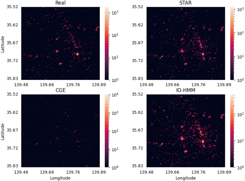
Figure 5: The geographical visualization of location visit frequency of real and simulated human trajectories on the TKY dataset.

5.7 RQ4: Visualization

The geographical visualization results of our proposed STAR method and two baseline methods on the TKY dataset are presented in Figure 5. The side colorbar illustrates the frequency of location visits, with brighter colors indicating higher visit frequencies. The STAR method yields more similar results in the diagonal direction’s highlighted areas to the real visit frequencies than the other two methods, namely CGE and IO-HMM, which are one of state-of-the-art deep learning methods and statistical modeling methods for trajectory simulation, respectively. Additionally, STAR also provides attention to lower-visited areas in the upper-left corner, while the other two methods lack precision in modeling the long-tailed location visit patterns.

6 Conclusion

In this paper, we propose a novel framework for human mobility simulation, namely SpatioTemporal-Augmented gRaph neural networks (STAR), to model the spatiotemporal effects among locations. On the one hand, STAR designs various kinds of spatiotemporal graphs to incorporate the spatiotemporal correspondences of locations, revealing the spatial proximity and functionality similarity with the temporal visit distribution. On the other hand, STAR builds the dual-branch decision generator module to balance the diverse transitions generated by the exploration branch and the repetitive patterns generated by the dwell branch. The STAR framework is optimized based on the classification rewards of the policy discriminator module after iteratively generating a complete trajectory sequence. We have conducted comprehensive experiments on the human mobility simulation task, verifying the superiority of the STAR framework to the state-of-the-art methods. Ablation studies on the multi-channel embedding module reveal that different datasets prefer different spatiotemporal graphs. Elaborate experiments further verify the effectiveness of the edges of the Vanilla version and the dwell branch.

However, deep learning-based models always suffer from data scarcity and sparsity, easily leading to overfitting in the small training data. In the future, we will explore the commonalities of different human mobility data and attempt to transfer the human mobility model from high-resource locations to low-resource locations. Another interesting direction is introducing massive external resources like daily social tweets to build a huge location graph, which can largely alleviate the data sparsity problem.

References

- [1] M. C. Gonzalez, C. A. Hidalgo, and A.-L. Barabasi, “Understanding individual human mobility patterns,” nature, vol. 453, no. 7196, pp. 779–782, 2008.
- [2] T. Althoff, R. Sosič, J. L. Hicks, A. C. King, S. L. Delp, and J. Leskovec, “Large-scale physical activity data reveal worldwide activity inequality,” Nature, vol. 547, no. 7663, pp. 336–339, 2017.
- [3] J. S. Jia, X. Lu, Y. Yuan, G. Xu, J. Jia, and N. A. Christakis, “Population flow drives spatio-temporal distribution of covid-19 in china,” Nature, vol. 582, no. 7812, pp. 389–394, 2020.
- [4] F. Xu, Y. Li, D. Jin, J. Lu, and C. Song, “Emergence of urban growth patterns from human mobility behavior,” Nature Computational Science, vol. 1, no. 12, pp. 791–800, 2021.
- [5] M. Bohm, M. Nanni, and L. Pappalardo, “Gross polluters and vehicle emissions reduction,” Nature Sustainability, pp. 1–9, 2022.
- [6] S. Venkatramanan, A. Sadilek, A. Fadikar, C. L. Barrett, M. Biggerstaff, J. Chen, X. Dotiwalla, P. Eastham, B. Gipson, D. Higdon et al., “Forecasting influenza activity using machine-learned mobility map,” Nature communications, vol. 12, no. 1, pp. 1–12, 2021.
- [7] J. Gao and B. C. O’Neill, “Mapping global urban land for the 21st century with data-driven simulations and shared socioeconomic pathways,” Nature communications, vol. 11, no. 1, pp. 1–12, 2020.
- [8] S. Chang, E. Pierson, P. W. Koh, J. Gerardin, B. Redbird, D. Grusky, and J. Leskovec, “Mobility network models of covid-19 explain inequities and inform reopening,” Nature, vol. 589, no. 7840, pp. 82–87, 2021.
- [9] L. Alessandretti, U. Aslak, and S. Lehmann, “The scales of human mobility,” Nature, vol. 587, no. 7834, pp. 402–407, 2020.
- [10] S. Gambs, M.-O. Killijian, and M. N. del Prado Cortez, “Next place prediction using mobility markov chains,” in Proceedings of the first workshop on measurement, privacy, and mobility, 2012, pp. 1–6.
- [11] M. Yin, M. Sheehan, S. Feygin, J.-F. Paiement, and A. Pozdnoukhov, “A generative model of urban activities from cellular data,” IEEE Transactions on Intelligent Transportation Systems, vol. 19, no. 6, pp. 1682–1696, 2017.
- [12] J. Feng, Y. Li, C. Zhang et al., “Predicting human mobility with attentional recurrent networks,” in Proceedings of the 2018 World Wide Web Conference on World Wide Web, pp. 1459–1468.
- [13] J. Feng, Z. Yang, F. Xu, H. Yu, M. Wang, and Y. Li, “Learning to simulate human mobility,” in Proceedings of the 26th ACM SIGKDD international conference on knowledge discovery & data mining, 2020, pp. 3426–3433.
- [14] Q. Gao, F. Zhou, T. Zhong, G. Trajcevski, X. Yang, and T. Li, “Contextual spatio-temporal graph representation learning for reinforced human mobility mining,” Information Sciences, 2022.
- [15] I. Goodfellow, J. Pouget-Abadie, M. Mirza, B. Xu, D. Warde-Farley, S. Ozair, A. Courville, and Y. Bengio, “Generative adversarial networks,” Communications of the ACM, vol. 63, no. 11, pp. 139–144, 2020.
- [16] D. Karamshuk, C. Boldrini, M. Conti, and A. Passarella, “Human mobility models for opportunistic networks,” IEEE Communications Magazine, vol. 49, no. 12, pp. 157–165, 2011.
- [17] A. Hess, K. A. Hummel, W. N. Gansterer, and G. Haring, “Data-driven human mobility modeling: a survey and engineering guidance for mobile networking,” ACM Computing Surveys (CSUR), vol. 48, no. 3, pp. 1–39, 2015.
- [18] J. Wang, X. Kong, F. Xia, and L. Sun, “Urban human mobility: Data-driven modeling and prediction,” ACM SIGKDD Explorations Newsletter, pp. 1–19, 2019.
- [19] H. Barbosa, M. Barthelemy, G. Ghoshal, C. R. James, M. Lenormand, T. Louail, R. Menezes, J. J. Ramasco, F. Simini, and M. Tomasini, “Human mobility: Models and applications,” Physics Reports, vol. 734, pp. 1–74, 2018.
- [20] S. Shin, H. Jeon, C. Cho, S. Yoon, and T. Kim, “User mobility synthesis based on generative adversarial networks: A survey,” in 2020 22nd International Conference on Advanced Communication Technology (ICACT). IEEE, 2020, pp. 94–103.
- [21] L. Pappalardo, S. Rinzivillo, Z. Qu, D. Pedreschi, and F. Giannotti, “Understanding the patterns of car travel,” The European Physical Journal Special Topics, vol. 215, no. 1, pp. 61–73, 2013.
- [22] L. Pappalardo, F. Simini, S. Rinzivillo, D. Pedreschi, F. Giannotti, and A.-L. Barabasi, “Returners and explorers dichotomy in human mobility,” Nature Communications, vol. 6, no. 1, p. 8166, 2015.
- [23] L. Alessandretti, P. Sapiezynski, V. Sekara, S. Lehmann, and A. Baronchelli, “Evidence for a conserved quantity in human mobility,” Nature Human Behaviour, vol. 2, no. 7, pp. 485–491, 2018.
- [24] L. Song, D. Kotz, R. Jain, and X. He, “Evaluating location predictors with extensive wi-fi mobility data,” ACM SIGMOBILE Mobile Computing and Communications Review, vol. 7, no. 4, pp. 64–65, 2003.
- [25] J. Krumm, E. Horvitz et al., “Locadio: Inferring motion and location from wi-fi signal strengths.” in mobiquitous, 2004, pp. 4–13.
- [26] L. Pappalardo and F. Simini, “Data-driven generation of spatio-temporal routines in human mobility,” Data Mining and Knowledge Discovery, vol. 32, no. 3, pp. 787–829, 2018.
- [27] C. Song, T. Koren, P. Wang, and A.-L. Barabási, “Modelling the scaling properties of human mobility,” Nature Physics, vol. 6, no. 10, pp. 818–823, 2010.
- [28] H. Barbosa, F. B. de Lima-Neto, A. Evsukoff, and R. Menezes, “The effect of recency to human mobility,” EPJ Data Science, vol. 4, pp. 1–14, 2015.
- [29] J. Toole, C. Herrera-Yague, C. Schneider, and M. C. Gonzalez, “Coupling human mobility and social ties,” Journal of the Royal Society Interface, vol. 12, 2015.
- [30] G. Cornacchia and L. Pappalardo, “Sts-epr: Modelling individual mobility considering the spatial, temporal, and social dimensions together,” Procedia Computer Science, vol. 184, pp. 258–265, 2021, the 12th International Conference on Ambient Systems, Networks and Technologies (ANT) / The 4th International Conference on Emerging Data and Industry 4.0 (EDI40) / Affiliated Workshops. [Online]. Available: https://www.sciencedirect.com/science/article/pii/S1877050921006645
- [31] S. Jiang, Y. Yang, S. Gupta, D. Veneziano, S. Athavale, and M. C. Gonzalez, “The timegeo modeling framework for urban mobility without travel surveys,” Proceedings of the National Academy of Sciences, vol. 113, p. 201524261, 2016.
- [32] S. Bengio, O. Vinyals, N. Jaitly, and N. Shazeer, “Scheduled sampling for sequence prediction with recurrent neural networks,” Advances in neural information processing systems, vol. 28, 2015.
- [33] L. Yu, W. Zhang, J. Wang, and Y. Yu, “Seqgan: Sequence generative adversarial nets with policy gradient,” in Proceedings of the AAAI conference on artificial intelligence, vol. 31, no. 1, 2017.
- [34] Y. Yuan, J. Ding, H. Wang, D. Jin, and Y. Li, “Activity trajectory generation via modeling spatiotemporal dynamics,” in Proceedings of the 28th ACM SIGKDD Conference on Knowledge Discovery and Data Mining, 2022, pp. 4752–4762.
- [35] V. Jakkula and D. J. Cook, “Mining sensor data in smart environment for temporal activity prediction,” Poster session at the ACM SIGKDD, San Jose, CA, 2007.
- [36] B. Minor, J. R. Doppa, and D. J. Cook, “Data-driven activity prediction: Algorithms, evaluation methodology, and applications,” in Proceedings of the 21th ACM SIGKDD International Conference on Knowledge Discovery and Data Mining, 2015, pp. 805–814.
- [37] J. Ye, Z. Zhu, and H. Cheng, “What’s your next move: User activity prediction in location-based social networks,” in Proceedings of the 2013 SIAM International Conference on Data Mining. SIAM, 2013, pp. 171–179.
- [38] N. Jaouedi, F. J. Perales, J. M. Buades, N. Boujnah, and M. S. Bouhlel, “Prediction of human activities based on a new structure of skeleton features and deep learning model,” Sensors, vol. 20, no. 17, p. 4944, 2020.
- [39] H. F. Nweke, Y. W. Teh, M. A. Al-Garadi, and U. R. Alo, “Deep learning algorithms for human activity recognition using mobile and wearable sensor networks: State of the art and research challenges,” Expert Systems with Applications, vol. 105, pp. 233–261, 2018.
- [40] J. Wang, X. Chen, F. Zhang, F. Chen, and Y. Xin, “Building load forecasting using deep neural network with efficient feature fusion,” Journal of Modern Power Systems and Clean Energy, vol. 9, no. 1, pp. 160–169, 2021.
- [41] N. Jia, “Application of data mining in intelligent power consumption,” IET Conference Proceedings, pp. 538–541(3), January 2012. [Online]. Available: https://digital-library.theiet.org/content/conferences/10.1049/cp.2012.1035
- [42] M. Defferrard, X. Bresson, and P. Vandergheynst, “Convolutional neural networks on graphs with fast localized spectral filtering,” in Proceedings of the 30th International Conference on Neural Information Processing Systems, 2016, pp. 3844–3852.
- [43] T. N. Kipf and M. Welling, “Semi-supervised classification with graph convolutional networks,” in International Conference on Learning Representations, 2017.
- [44] W. Hamilton, Z. Ying, and J. Leskovec, “Inductive representation learning on large graphs,” in Proceddings of the 31st International Conference on Neural Information Processing Systems, 2017, pp. 1024–1034.
- [45] P. Velickovic, G. Cucurull, A. Casanova, A. Romero, P. Lio, and Y. Bengio, “Graph attention networks,” in International Conference on Learning Representations, 2018.
- [46] A. Vaswani, N. Shazeer, N. Parmar, J. Uszkoreit, L. Jones, A. N. Gomez, Ł. Kaiser, and I. Polosukhin, “Attention is all you need,” in Proceedings of the 31st International Conference on Neural Information Processing Systems, 2017, pp. 5998–6008.
- [47] Y. Zheng, L. Capra, O. Wolfson, and H. Yang, “Urban computing: concepts, methodologies, and applications,” ACM Transactions on Intelligent Systems and Technology (TIST), vol. 5, no. 3, pp. 1–55, 2014.
- [48] Z. Pan, W. Zhang, Y. Liang, W. Zhang, Y. Yu, J. Zhang, and Y. Zheng, “Spatio-temporal meta learning for urban traffic prediction,” IEEE Transactions on Knowledge and Data Engineering, vol. 34, no. 3, pp. 1462–1476, 2020.
- [49] L. Wang, D. Chai, X. Liu, L. Chen, and K. Chen, “Exploring the generalizability of spatio-temporal traffic prediction: meta-modeling and an analytic framework,” IEEE Transactions on Knowledge and Data Engineering, 2021.
- [50] X. Liu, Z. Zhang, L. Lyu, Z. Zhang, S. Xiao, C. Shen, and S. Y. Philip, “Traffic anomaly prediction based on joint static-dynamic spatio-temporal evolutionary learning,” IEEE Transactions on Knowledge and Data Engineering, vol. 35, no. 5, pp. 5356–5370, 2022.
- [51] W. Zeng, C. Lin, K. Liu, J. Lin, and A. K. Tung, “Modeling spatial nonstationarity via deformable convolutions for deep traffic flow prediction,” IEEE Transactions on Knowledge and Data Engineering, 2021.
- [52] Y. Gong, Z. Li, J. Zhang, W. Liu, and Y. Zheng, “Online spatio-temporal crowd flow distribution prediction for complex metro system,” IEEE Transactions on knowledge and data engineering, vol. 34, no. 2, pp. 865–880, 2020.
- [53] S. Wang, J. Cao, and P. Yu, “Deep learning for spatio-temporal data mining: A survey,” IEEE transactions on knowledge and data engineering, 2020.
- [54] S. Agarwal, R. Sawhney, M. Thakkar, P. Nakov, J. Han, and T. Derr, “Think: Temporal hypergraph hyperbolic network,” in ICDM. IEEE, 2022, pp. 849–854.
- [55] Y. Qin, Y. Fang, H. Luo, F. Zhao, and C. Wang, “Dmgcrn: Dynamic multi-graph convolution recurrent network for traffic forecasting,” arXiv preprint arXiv:2112.02264, 2021.
- [56] S. Guo, Y. Lin, N. Feng, C. Song, and H. Wan, “Attention based spatial-temporal graph convolutional networks for traffic flow forecasting,” in Proceedings of the AAAI conference on artificial intelligence, vol. 33, no. 01, 2019, pp. 922–929.
- [57] C. Song, Y. Lin, S. Guo, and H. Wan, “Spatial-temporal synchronous graph convolutional networks: A new framework for spatial-temporal network data forecasting,” in AAAI, vol. 34, no. 01, 2020, pp. 914–921.
- [58] M. Li and Z. Zhu, “Spatial-temporal fusion graph neural networks for traffic flow forecasting,” in AAAI, vol. 35, no. 5, 2021, pp. 4189–4196.
- [59] T. Wang, J. Chen, J. Lu, K. Liu, A. Zhu, H. Snoussi, and B. Zhang, “Synchronous spatiotemporal graph transformer: A new framework for traffic data prediction,” IEEE Transactions on Neural Networks and Learning Systems, 2022.
- [60] V. M. Panaretos and Y. Zemel, “Statistical aspects of wasserstein distances,” Annual review of statistics and its application, vol. 6, pp. 405–431, 2019.
- [61] K. Cho, B. Van Merrienboer, D. Bahdanau, and Y. Bengio, “On the properties of neural machine translation: Encoder-decoder approaches,” arXiv preprint arXiv:1409.1259, 2014.
- [62] R. J. Williams, “Simple statistical gradient-following algorithms for connectionist reinforcement learning,” Reinforcement learning, pp. 5–32, 1992.
- [63] S. Hochreiter and J. Schmidhuber, “Long short-term memory,” Neural computation, vol. 9, no. 8, pp. 1735–1780, 1997.
- [64] S. Feng, G. Cong, B. An, and Y. M. Chee, “Poi2vec: Geographical latent representation for predicting future visitors,” in Proceedings of the AAAI Conference on Artificial Intelligence, vol. 31, no. 1, 2017.
- [65] K. Ouyang, R. Shokri, D. S. Rosenblum, and W. Yang, “A non-parametric generative model for human trajectories.” in IJCAI, vol. 18, 2018, pp. 3812–3817.
- [66] B. Fuglede and F. Topsoe, “Jensen-shannon divergence and hilbert space embedding,” in International symposium onInformation theory, 2004. ISIT 2004. Proceedings. IEEE, 2004, p. 31.
- [67] A. Paszke, S. Gross, F. Massa, A. Lerer, J. Bradbury, G. Chanan, T. Killeen, Z. Lin, N. Gimelshein, L. Antiga et al., “Pytorch: An imperative style, high-performance deep learning library,” in Proceedings of the 33th International Conference on Neural Information Processing Systems, 2019, pp. 8026–8037.