On some one-dimensional quantum-mechanical models with a delta-potential interaction

Abstract

We discuss a systematic construction of dimensionless quantum-mechanical equations. The process reduces the number of independent model parameters to a minimum and, at the same time, provides the natural units of length, energy, etc. in a clear, straightforward way. We compare this systematic procedure with the widely adopted one that consists of setting $\hbar=1$. As illustrative examples, we choose some simple one-dimensional models proposed recently for the study of localized states in inhomogeneous media.

1 Introduction

In a recent paper Savotchenko[1] discussed “localized states in the constant-index and graded-index media separated by thin defect layer” in terms of exactly solvable one-dimensional quantum-mechanical models. In particular he considered the influence of the intensity of local interaction the excitations with the interface in short-range approximation on the field localization” and obtained “the exact dependencies of localization energy on the interface interaction intensity”. In order to solve the Schrödinger equation Savotchenko chose some sort of “conventional dimensionless units” based on setting $\hbar=1$. As a result he was forced to give values to six model parameters in order to obtain his results. In this paper we resort to a well known recipe for deriving suitable dimensionless equations[2] and compare both kind of calculations.

In section 2 we derive a dimensionless equation for a sufficiently general quantum-mechanical model and obtain the quantization condition. In section 3 we consider a linear potential and in section 4 the parabolic and exponential potentials. Finally, in section5 we review the main results and draw conclusions.

2 General model

The models discussed by Savotchenko[1] are particular cases of the one-dimensional Schrödinger equation

$$\psi^{\prime\prime}(x)=\frac{2m}{\hbar^{2}}\left[V(x)-E\right]\psi(x).$$ (1)

In order to obtain a dimensionless equation we define $q=x/L$, where $L$ is the unit of length defined conveniently for each model[2]. We thus obtain the eigenvalue equation

$$\varphi^{\prime\prime}(q) = 2\left[v(q)-\epsilon\right]\varphi(q),$$

$$\varphi(q) = \psi(Lq),\;v(q)=\frac{mL^{2}}{\hbar^{2}}V(Lq),\;\epsilon=\frac{mL^{2}}{\hbar^{2}}E.$$ (2)

We are interested in potential-energy functions of the form

$$V(x)=U_{0}\delta(x)+U(x),$$ (3)

where $\delta(x)$ is the Dirac delta function. The dimensionless potential becomes

$$v(q) = u_{0}\delta(q)+u(q),$$

$$u_{0} = \frac{mL}{\hbar^{2}}U_{0},\;u(q)=\frac{mL^{2}}{\hbar^{2}}U(Lq).$$ (4)

The delta interaction forces a discontinuity of the first derivative of the solution at origin

$$\int_{0^{-}}^{0^{+}}\varphi^{\prime\prime}(q)\,dq=\varphi^{\prime}(0^{+})-\varphi^{\prime}(0^{-})=2u_{0}\varphi(0).$$ (5)

In particular we focus on the piecewise potential

$$U(x)=\left\{\begin{array}[]{c}U_{L}(x),\;x<0\\ U_{R}(x),\;x>0\end{array}\right.,$$ (6)

that leads to

$$\varphi_{L}^{\prime\prime}(q) = 2\left[u_{L}(q)-\epsilon\right]\varphi_{L}(q),\;\lim\limits_{q\rightarrow-\infty}\varphi_{L}(q)=0,$$

$$\varphi_{R}^{\prime\prime}(q) = 2\left[u_{R}(q)-\epsilon\right]\varphi_{R}(q),\;\lim\limits_{q\rightarrow\infty}\varphi_{R}(q)=0,$$

$$u_{L}(q) = \frac{mL^{2}}{\hbar^{2}}U_{L}(Lq),\;u_{R}(q)=\frac{mL^{2}}{\hbar^{2}}U_{R}(Lq).$$ (7)

It follows from $\varphi_{L}(0)=\varphi_{R}(0)=\varphi(0)$ and equation (5) that

$$\frac{\varphi_{R}^{\prime}(0)}{\varphi_{R}(0)}-\frac{\varphi_{L}^{\prime}(0)}{\varphi_{L}(0)}=2u_{0}.$$ (8)

If we choose $U_{L}^{\prime}=0$ and $U_{R}^{\prime}\neq 0$ we have

$$\frac{\varphi_{L}(q)}{\varphi_{L}(0)}=e^{\alpha q},\;\alpha=\sqrt{2\left(u_{L}-\epsilon\right)},$$ (9)

and the quantization condition

$$\frac{\varphi_{R}^{\prime}(0)}{\varphi_{R}(0)}-\alpha=2u_{0}.$$ (10)

3 First example

One of the simplest potentials that we can choose for $x>0$ is

$$U_{R}(x)=A+Bx,\;B>0,$$ (11)

that leads to

$$u_{R}(q)=\frac{mL^{2}}{\hbar^{2}}A+\frac{mL^{3}}{\hbar^{2}}Bq.$$ (12)

Upon choosing $L^{3}=\hbar^{2}/(2mB)$ and defining $a=mL^{2}A/\hbar^{2}$ we have $u_{R}(q)=a+q/2$ and the corresponding right eigenvalue equation

$$\varphi_{R}^{\prime\prime}(q)-\left(\delta+q\right)\varphi_{R}(q)=0,\;\delta=2a-2\epsilon,$$ (13)

that can be transformed into the Airy equation[3] $Y^{\prime\prime}(z)-zY(z)=0$ for the variable $z=q+\delta$. Therefore, the solution for $q>0$ is

$$\varphi_{R}(q)=Ai(q+\delta),$$ (14)

and the quantization condition becomes

$$\frac{Ai^{\prime}(\delta)}{Ai(\delta)}=2u_{0}+\sqrt{\delta+\gamma},\;\gamma=2\left(u_{L}-a\right).$$ (15)

Note that the solutions depend on only two relevant model parameters, $u_{0}$ and $\gamma$. This is one of the advantages of using suitable dimensionless equations[2]. On the other hand, Savotchenko[1] was forced to give values to $m$ and five model parameters.

Figure 1 shows both sides of equation (15) for some values of $u_{0}$ and $\gamma$. The intersections give us the values of $\delta$ for the bound states. We appreciate that the number of bound states decreases with $u_{0}$ and increases with $\gamma$. There are bound states even in the absence of the delta potential (cases (c) and (d)) because $U(x)$ is a well when $\gamma>0$.

For a given suitable pair of values of $u_{0}$ and $\gamma$ we obtain a series of roots $\delta_{j}$, $j=1,2,\ldots,k$ from which we derive the dimensionless energies and eigenfunctions

$$\epsilon_{j} = a-\frac{\delta_{j}}{2},$$

$$\varphi_{j}(q) = \varphi_{j}(0)\left\{\begin{array}[]{l}e^{\alpha_{j}q},\;\alpha_{j}=\sqrt{\delta_{j}+\gamma},\;q<0\\ Ai\left(q+\delta_{j}\right)/Ai\left(\delta_{j}\right),\;q>0\end{array}\right..$$ (18)

For example, when $u_{0}=1$ and $\gamma=10$ we have: $\delta_{1}=-2.136182406$, $\delta_{2}=-3.877567571$, $\delta_{3}=-5.301530405$, $\delta_{4}=-6.557969140$, $\delta_{5}=-7.703603791$, $\delta_{6}=-8.766062952$ and $\delta_{7}=-9.753634587$. Note that we only set two independents parameters, $u_{0}$ and $\gamma$, and obtain solutions for an infinite set of values of $m$, $U_{L}$, $A$ and $B$. This is one of the great advantages of using dimensionless equations[2]. This results suggest that the role of the thickness parameter[1] (which is here absorbed into $u_{0}$ and $\gamma$, through $B$) may not be so relevant for the discussion of the bound states.

4 Other examples

For the second example we consider a parabolic potential

$$U_{R}(x)=A+Bx^{2},$$ (19)

and choose the unit of length $L=\hbar^{1/2}/\left(mB\right)^{1/4}$ so that

$$u_{R}(q) = a+q^{2},$$

$$a = \frac{mL^{2}}{\hbar^{2}}A=\sqrt{\frac{m}{B}}\frac{A}{\hbar}.$$ (20)

The eigenvalue equation for $q>0$ becomes

$$\varphi_{R}^{\prime\prime}(\delta,q)-\left(\delta+2q^{2}\right)\varphi_{R}(\delta,q)=0,\;\delta=2(a-\epsilon),$$ (21)

that leads to the quantization condition

$$\frac{\varphi_{R}^{\prime}(\delta,0)}{\varphi_{R}(\delta,0)}=2u_{0}+\sqrt{\gamma+\delta},\;\gamma=2\left(u_{L}-a\right).$$ (22)

The solution $\varphi_{R}(\delta,q)$ can be expressed in terms of the Whittaker functions[1, 3] but the explicit calculation is not relevant for present purposes. The main point is that, as in the preceding example, there are only two independent parameters that completely determine both the eigenvalues and eigenfunctions. On the other hand, Savotchenko[1] was forced to give values to $m$ and five model parameters.

The third model is given by the exponential potential

$$U_{R}(x)=A+Be^{\beta x},\;B>0,\;\beta>0.$$ (23)

In this case we arbitrarily choose $L=1/\beta$ so that

$$u_{R}(q)=a+be^{q},\;a=\frac{mA}{\hbar^{2}\beta^{2}},\;b=\frac{mB}{\hbar^{2}\beta^{2}},$$ (24)

and

$$\varphi_{R}^{\prime\prime}(b,\delta,q)-\left(\delta+2be^{q}\right)\varphi_{R}(b,\delta,q)=0,\;\delta=2(a-\epsilon).$$ (25)

The solution to this equation can be expressed in terms of Bessel functions[1, 3] and the quantization condition becomes

$$\frac{\varphi_{R}^{\prime}(b,\delta,0)}{\varphi_{R}(b,\delta,0)}=2u_{0}+\sqrt{\gamma+\delta},\;\gamma=2\left(u_{L}-a\right).$$ (26)

In this case we have three independent parameters that completely determine the eigenvalues and eigenfunctions. On the other hand, Savotchenko[1] was forced to give values to $m$ and five model parameters.

5 Conclusions

Throughout this paper we have shown that the appropriate construction of dimensionless equations simplify the problem enormously providing the actual units of length, energy, etc. in a clear, straightforward way . In the examples discussed above the dimensionless eigenvalue equations exhibit either two or three independent model parameters instead of the six parameters that remain when one simply sets $\hbar=1$[1]. Other illustrative examples of dimensionless equations in nonrelativistic quantum mechanics and quantum chemistry are discussed elsewhere[2].

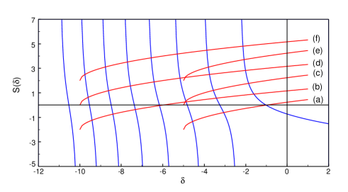
Figure 1: $S(\delta)=A_{i}^{\prime}(\delta)/A_{i}(\delta)$ (blue line) and $S(\delta)=u_{0}+\sqrt{\delta+\gamma}$ (red line) for (a) ($u_{0}=-1$, $\gamma=5$), (b) ($u_{0}=-1$, $\gamma=10$), (c) ($u_{0}=0$, $\gamma=5$), (d) ($u_{0}=0$, $\gamma=10$), (e) ($u_{0}=1$, $\gamma=5$), (f) ($u_{0}=1$, $\gamma=10$)

References

• [1] S. E. Savotchenko, Eur. Phys. J. Plus 138 (2023) 390.
• [2] F. M. Fernández, Dimensionless equations in non-relativistic quantum mechanics, arXiv:2005.05377 [quant-ph]
• [3] M. Abramowitz and I. A. Stegun, Handbook of Mathematical Functions, Dover, New York, 1972.
Refer to caption