Stability analysis of warm quintessential dark energy model

Abstract

A dynamical system analysis is performed for a model of dissipative quintessential inflation realizing warm inflation at early primordial times and dissipative interations in the dark sector at late times. The construction makes use of a generalized exponential potential realizing both phases of accelerated expansion. A focus is given on the behavior of the dynamical system at late times and the analysis is exemplified by both analytical and numerical results. The results obtained demonstrate the viability of the model as a quintessential inflation model in which stable solutions can be obtained.

I Introduction

Cosmic inflation Kazanas:1980tx ; Guth:1980zm ; Sato:1981ds ; Sato:1980yn ; Linde:1981mu ; Albrecht:1982wi , proposed as a solution to the fine-tuning problems of the Big Bang theory, describes an accelerated expanding phase in the early Universe. It is also commonly assumed to be driven by a potential energy dominated scalar field, called the inflaton. On the other hand, the observational discovered late-time cosmic acceleration of our Universe SupernovaCosmologyProject:1998vns ; SupernovaSearchTeam:1998fmf can also be explained by the dynamics of a scalar field, called the quintessence Peebles:1987ek ; Ratra:1987rm (for reviews, see, e.g., Bamba:2012cp ; Tsujikawa:2013fta ). There has been constant effort in the literature to unify the early- and the late-time cosmic accelerations by making the same scalar field play the role of both the inflaton and the quintessence field (for recent reviews, see deHaro:2021swo ; Bettoni:2021qfs and references therein). However, the main obstacle to unify the early- and the late-time accelerations by a single scalar field is that, as in conventional cold inflation, the energy density in the inflaton field must, at least partially, decay to radiation at the end of inflation in order to reheat the Universe, while part of the energy density of the inflaton must survive until recently if the inflaton should also play the role of quintessence. To overcome this difficulty, a number of alternative reheating mechanisms have been proposed, such as gravitational reheating Ford:1986sy ; Chun:2009yu , instant preheating Felder:1998vq ; Campos:2002yk , curvaton reheating Feng:2002nb ; BuenoSanchez:2007jxm , non-minimal Dimopoulos:2018wfg or Ricci reheating Bettoni:2018utf ; Opferkuch:2019zbd , just to cite some examples.

Another novel way of overcoming the reheating problem in such unified models is to opt for warm inflation (WI) Berera:1995ie as the inflationary model (for recent reviews on WI, see, e.g., Kamali:2023lzq ; Berera:2023liv ). WI is a variant inflationary scenario where the inflaton field, having strong couplings with other fields, dissipates its energy to a thermal bath during inflation. As a constant thermal bath is maintained throughout WI, it smoothly ends in a radiation dominated Universe, without invoking the need of a separate reheating phase. Thus, WI can naturally alleviate the problem of reheating in such unified quintessential inflation models. Besides, the constraints set by the swampland conjectures (especially the de Sitter conjecture Ooguri:2018wrx ; Garg:2018reu ), which prohibit constructions of de Sitter vacua in string theory, cannot be easily met by the conventional inflationary models Agrawal:2018own ; Kinney:2018nny . WI, however, naturally overcome those constraints Das:2018hqy ; Motaharfar:2018zyb ; Das:2018rpg ; Berera:2023mlj and, thus, can be considered as a viable inflationary paradigm in string landscapes. On the late-time acceleration front, quintessence is in better agreement with the swampland conjectures than a non-zero cosmological constant $\Lambda$ Agrawal:2018own . Hence, unifying WI with quintessence has an added advantage even from the point of view of effective field theories consistent with a quantum gravity ultraviolet realization.

The first two attempts Dimopoulos:2019gpz ; Rosa:2019jci made in the literature to unify WI with late-time quintessence-driven acceleration, dissipative effects played a role only during the early-time inflationary phase, after which they die down when WI ends. Afterwards, it was assumed that the late-time acceleration was driven by standard quintessence dynamics, where the quintessence field is treated to be decoupled from the rest of the matter in the Universe. Above all, two different forms of potentials of the same scalar field are required to drive the two accelerating phases, at early- and at late-times, in these models. There has been another novel attempt to unify WI and the late-time acceleration Lima:2019yyv , where the scalar field first dissipates its energy to a radiation bath during inflation and, at a later stage, due to couplings with matter, it dissipates its energy to the matter content of the Universe. This non-relativistic matter content, generated due to the dissipation of the scalar field, is shown to be able to account for the dark matter in the Universe. Besides, in the implementation considered in Ref. Lima:2019yyv only one form of the scalar potential (a generalized form of exponential potential) is required to drive both the early- and the late-time accelerations, which is an added advantage. Thus, this model accounts for inflation, dark matter and dark energy at one go.

The main feature of WI, which distinguishes it from the standard inflationary paradigm, is the dissipative effects of the inflaton field during inflation. The presence of dissipation makes WI a rich dynamical system, whose stability in the early Universe has been previously analyzed in the literature deOliveira:1997jt ; Moss:2008yb ; delCampo:2010by ; Bastero-Gil:2012vuu ; Li:2018sfs . However, a study of how a similar analysis could be carried out when those dissipative effects can extend up to the late-times, is still largely missing. In the unified model described in Lima:2019yyv , dissipation effects are effective even after the inflationary phase, and interactions in the post-inflationary epoch are motivated fully from the WI picture. Though this might have similarities with models describing interactions in the dark sector (see, e.g., the review papers Bolotin:2013jpa ; Wang:2016lxa ), the model studied here is, however, much more reminiscent of the WI idea, but extending it to quintessential inflation models. Therefore, we will call the late-time acceleration of this model as warm quintessential dark energy model. The aim of this paper is to perform the first study in the literature of the stability of the dynamical system of this warm quintessential dark energy model.

We have organized this paper as follows. In Sec. II, we discuss the model whose stability we want to determine in this paper. In Sec. III, we discuss the dynamical system produced by the model and show that it indeed accounts for four different phases of evolution: (a) inflation, (b) radiation domination, (c) matter domination and (d) dark energy domination for some generic choices of parameters. In Sec. IV, we qualitatively show that the late-time acceleration is an attractor solution of the model. In the following section, Sec. V, we perform a rigorous dynamical system analysis to study the stability of the system depending on different model parameters. In Sec. VI, we discuss our main results and conclude. Finally, an Appendix is included where we also study the stability of the slow-roll trajectories in both early- and late-time epochs.

II Model

In our model, the quintessential scalar field decays to both radiation and matter energy densities. Here, we propose the complete set of background equations involving the quintessential scalar field $\phi$, the radiation fluid energy density $\rho_{r}$ and the matter energy density $\rho_{m}$, with evolution equations as given, respectively, by

$$\ddot{\phi}+3H\dot{\phi}+\Upsilon_{r}\dot{\phi}+\Upsilon_{m}\dot{\phi}+V_{,\phi}=0,$$ (1)

$$\dot{\rho}_{r}+4H\rho_{r}=\Upsilon_{r}\dot{\phi}^{2},$$ (2)

$$\dot{\rho}_{m}+3H\rho_{m}=\Upsilon_{m}\dot{\phi}^{2},$$ (3)

where $V_{,\phi}$ is the field derivative of the quintessential scalar potential, $\Upsilon_{r}$ describes the energy exchange between the quintessential scalar field and radiation energy density, $\Upsilon_{m}$ describes the energy exchange between the quintessential scalar field and matter energy density and the Hubble parameter is given by the Friedmann equation,

$$H^{2}\equiv\frac{\dot{a}^{2}}{a^{2}}=\frac{1}{3M_{\rm Pl}^{2}}\left(\frac{\dot{\phi}^{2}}{2}+V+\rho_{r}+\rho_{m}\right),$$ (4)

with $a$ the scale factor and $M_{\rm Pl}\equiv(8\pi G)^{-\frac{1}{2}}\simeq 2.44\times 10^{18}$ GeV is the reduced Planck mass and $G$ is Newton’s gravitational constant.

We parametrize the dissipation terms $\Upsilon_{r}$ and $\Upsilon_{m}$ in the following generic forms, which are motivated from many early works on WI and also discussed in Ref. Lima:2019yyv ,

$$\Upsilon_{r}=C_{r}\rho_{R}^{c/4}\phi^{p}M^{1-c-p},$$ (5)

and

$$\Upsilon_{m}=C_{m}\rho_{m}^{k/4}\phi^{q}M^{1-k-q},$$ (6)

where $C_{r}$ and $C_{m}$ are dimensionless constants and $M$ is some appropriate (constant) scale with mass dimension. Hence, $[\Upsilon_{r}]=M$ and $[\Upsilon_{m}]=M$ . The various powers $c,\;p,\;k,\;q$ model the different dependencies that these dissipation coefficients might have with the quintessence background field, radiation energy density and matter energy density. These parameters are not all arbitrary and the stability of the dynamical system can put strong bounds on them, as we will see. In particular, the stability of the system under slow-roll demands that $|c|<4$ and $|k|<4$ (see the Appendix A for details).

Appropriate choices of dependencies on $\phi$, $\rho_{r}$ and $\rho_{m}$ can be made in Eqs. (5) and (6) such that we can have, for example, the dissipation coefficient $\Upsilon_{r}$, given in Eq. (5), dominating during inflation, thus leading to a WI regime, while $\Upsilon_{m}$, given in Eq. (6), only dominates at late times Lima:2019yyv . While $\Upsilon_{m}$ can be subdominant at primordial times, it can help in setting an initial abundance for the matter density. Given appropriate parameters $C_{m}$ and $M$, we can arrange for the matter-quintessence scalar field to display a similar behaviour found, e.g., in the case of nonminimal couplings of the scalar field to matter Amendola:1999er , thus modelling different energy exchange forms between the dark sector components. The matter-quintessence scalar field interaction term, under appropriate choices of parameters, can also help in providing an extra friction force on the quintessence scalar field and, thus, help making $\phi$ acquire a negative equation of state at late times, signalling the beginning of the dark energy (quintessence) domination epoch and even making scalar fields with steeper potentials more likely to work as a quintessence field, as we will see later.

III The dynamical system

The evolution equations (1) - (3) can be brought into a form appropriate for a dynamical system analysis by defining the variables Bahamonde:2017ize

$$x=\frac{\dot{\phi}}{\sqrt{6}M_{\rm Pl}H},$$ (7)

$$y=\sqrt{\frac{V}{3}}\frac{1}{M_{\rm Pl}H},$$ (8)

$$\Omega_{r}=\frac{\rho_{r}}{3M_{\rm Pl}^{2}H^{2}},$$ (9)

$$\Omega_{m}=\frac{\rho_{m}}{3M_{\rm Pl}^{2}H^{2}}.$$ (10)

Note that from the above definitions, we have that

$$x^{2}+y^{2}=\Omega_{\phi},$$ (11)

is the fraction in energy density of the quintessence scalar field. From Eqs. (7) - (10), the Friedmann equation (4) becomes equivalent to

$$1=x^{2}+y^{2}+\Omega_{r}+\Omega_{m}.$$ (12)

The evolution equations (1) - (3) can then be brought into a dynamical system form as

$$x^{\prime} = -\frac{3x(1-x^{2})}{2}+\frac{\Omega_{r}x}{2}-3x(Q_{m}+Q_{r})$$ (13)

$$+ \sqrt{\frac{3}{2}}\lambda y^{2}-\frac{3xy^{2}}{2},$$

$$y^{\prime} = \frac{3y}{2}+\frac{3x^{2}y}{2}-\frac{3y^{3}}{2}-\sqrt{\frac{3}{2}}xy\lambda+\frac{y\Omega_{r}}{2},$$ (14)

$$\lambda^{\prime} = -\sqrt{6}x(-1+\Gamma)\lambda^{2},$$ (15)

$$\Omega_{r}^{\prime} = 6x^{2}Q_{r}-\Omega_{r}+3x^{2}\Omega_{r}-3y^{2}\Omega_{r}+\Omega_{r}^{2},$$ (16)

where, in the above equations, a prime means derivative with respect to the number of efolds, ${}^{\prime}\equiv d/dN$, where $dN=Hdt$, while $Q_{r}$ and $Q_{m}$ are the dissipation ratios, defined as

$$Q_{r}=\frac{\Upsilon_{r}}{3H},$$ (17)

and

$$Q_{m}=\frac{\Upsilon_{m}}{3H}.$$ (18)

In Eqs. (13) - (16) we have also introduced the variable $\lambda$, which is defined as

$$\lambda=-M_{\rm Pl}\frac{V_{,\phi}(\phi)}{V(\phi)},$$ (19)

and $\Gamma$ in Eq. (15) is defined as

$$\Gamma=\frac{V(\phi)V_{,\phi\phi}(\phi)}{V_{,\phi}^{2}(\phi)}.$$ (20)

Note that the Eqs. (13) - (16) are general and valid in principle for any potential. To complete the dynamical system, we also need the evolution equations for the dissipation ratios $Q_{m}$ and $Q_{r}$ and to fix the form of the inflaton potential $V(\phi)$. For definiteness, let us consider the generalized exponential inflaton potential of the form:

$$V(\phi)=V_{0}e^{-\alpha(\phi/M_{\rm Pl})^{n}},$$ (21)

where $V_{0}$ is the normalization of the potential, $\alpha$ is a dimensionless constant here taken as positive and $n>1$ for potentials steeper than the simple exponential potential. This form of potential was originally proposed in Ref. Geng:2015fla and considered also in Refs. Geng:2017mic ; Ahmad:2017itq ; Shahalam:2017rit ; Das:2019ixt for quintessential inflation in the cases of absence of dissipation (i.e., radiation production). The first use of this potential in the context of warm quintessential inflation was in Ref. Lima:2019yyv and later also considered in Refs. Gangopadhyay:2020bxn ; Basak:2021cgk . Studies involving observational predictions for this model in the context of WI were developed in Refs. Das:2020xmh ; Das:2022ubr .

From the potential (21), we then obtain that

$$\Gamma=1-\frac{(n-1)}{n\alpha}\left(\frac{\lambda}{n\alpha}\right)^{\frac{n}{1-n}},$$ (22)

and

$$\lambda=n\alpha\left(\frac{\phi}{M_{\text{Pl}}}\right)^{n-1}.$$ (23)

Note that for $n\neq 1$, $\phi$ is related to $\lambda$ by

$$\phi=M_{\rm Pl}\left(\frac{\lambda}{n\alpha}\right)^{\frac{1}{n-1}}.$$ (24)

From the above definitions, the evolution equations for $Q_{m}$ and $Q_{r}$ can be expressed, respectively, as

$$Q_{m}^{\prime} = \frac{3(2-k)Q_{m}}{4}+\frac{3(x^{2}-y^{2})Q_{m}}{2}$$ (25)

$$+ \sqrt{6}qx\left(\frac{n\alpha}{\lambda}\right)^{\frac{1}{-1+n}}Q_{m}+\frac{Q_{m}\Omega_{r}}{2}$$

$$- \frac{3kx^{2}Q_{m}^{2}}{2\left(-1+x^{2}+y^{2}+\Omega_{r}\right)},$$

$$Q_{r}^{\prime} = \frac{3(1-2c)Q_{r}}{2}+\frac{3(x^{2}-y^{2})Q_{r}}{2}$$ (26)

$$+ \sqrt{6}px\left(\frac{n\alpha}{\lambda}\right)^{\frac{1}{-1+n}}Q_{r}+\frac{3cx^{2}Q_{r}^{2}}{2\Omega_{r}}$$

$$+ \frac{Q_{r}\Omega_{r}}{2}.$$

In writing the system of equations Eqs. (13) - (16), (25) and (26), we have considered the fraction in energy density in matter as equivalently to the first integral of Eq. (3) and which is determined through the constraint Eq. (12). The system of equations Eqs. (13) - (16), (25) and (26), together with Eq. (12), hence, form a complete set of equations describing the dynamics of the system.

In Ref. Lima:2019yyv , the evolution equations (1) - (3) were solved assuming a dissipation coefficient $\Upsilon_{r}$ given by

$$\Upsilon_{r}=C_{r}\rho_{r}^{3/4}/\phi^{2},$$ (27)

while $\Upsilon_{m}$ was taken to be of the form $\Upsilon_{m}=\Upsilon_{m,1}+\Upsilon_{m,2}$, where

$$\Upsilon_{m,1} = C_{m}\rho_{m}^{3/4}/\phi^{2},$$ (28)

$$\Upsilon_{m,2} = M^{2}/\rho_{m}^{1/4}.$$ (29)

Let us show that in this case, the dynamical system given by Eqs. (13) - (16), (25) and (26) lead to the same dynamics as shown in Ref. Lima:2019yyv . In Fig. 1 we show the result obtained by the solution of the dynamical system for the energy density fractions $\Omega_{\phi},\,\Omega_{r}$ and $\Omega_{m}$ and which is obtained by a representative example of initial conditions. We see that the system of equations (13) - (16), (25) and (26) produce an evolution that is initially characterized by an accelerated inflationary regime, when $\Omega_{\phi}$ dominates. This phase smoothly goes to a radiation dominated regime when $\Omega_{r}$ dominates. Towards the end of the evolution, it displays a short matter dominated phase, before $\Omega_{\phi}$ becomes the dominating component again in the future, which corresponds to a dark energy phase.

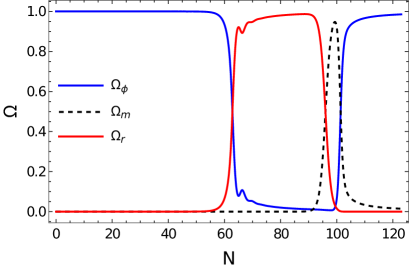
Figure 1: The energy density ratios as a function of the number of e-folds fos an inflaton potential with constants $n=3$ and $\alpha=0.015$. The initial conditions considered were such that $x(0)=0.0025,\,\Omega_{m}(0)=10^{-50},\,\Omega_{r}(0)=5.8\times 10^{-10},\,\lambda(0)=6.1\times 10^{-3}$, while for the dissipation coefficient ratios we have considered $Q_{r}(0)=10^{-4}$, $Q_{m,1}(0)=1.2\times 10^{-40}$ for the ratio corresponding to the dissipation coefficient $\Upsilon_{m,1}$ and $Q_{m,2}(0)=1.7\times 10^{-65}$ for the dissipation coefficient $\Upsilon_{m,2}$ (the combination of the two dissipation coefficients were considered such to reproduce the analogous case of Ref. Lima:2019yyv ).

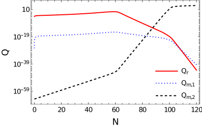
Figure 2: The evolution of the dissipation ratios $Q_{r}$, $Q_{m,1}$ and $Q_{m,2}$.

In Fig. 2, we give the evolution of the dissipation ratios $Q_{r}$, $Q_{m,1}$ and $Q_{m,2}$ obtained from Eqs. (27), (28) and (29). Note that right after inflation both $Q_{r}$ and $Q_{m,1}$ drop similarly, while $Q_{m,2}$ is enhanced after inflation, during the radiation era, while flattening at late times. This shows that different choices of the powers in Eqs. (5) and (6), can lead to different evolutions during different epochs in the universe.

IV Late time dynamics: A qualitative analysis

Analyzing the complete dynamical system made of the Eqs. (13) - (16), (25) and (26) is too complicated given that it is a six-dimensional order system. However, we can still get valuable information looking at snapshots of the system on a given plane. The most interesting plane to look at is the plane $(x,y)$, which gives us information about the behavior of the trajectories passing through the accelerated region. This is of particular importance when studying the late-time dynamics of the system, where we want to know about the ability of the system in reaching a DE dominated regime. We perform this analysis next, and leave the full dynamical system analysis of the late-time dynamics for the next section.

Since we are interested in the late-time behavior of the system, we can ignore the radiation related terms in Eqs. (13) and (14), which can then be approximated as

$$x^{\prime} \simeq -\frac{3x(1-x^{2})}{2}-3xQ_{m}$$ (30)

$$+ \sqrt{\frac{3}{2}}\lambda y^{2}-\frac{3xy^{2}}{2},$$

$$y^{\prime} \simeq \frac{3y}{2}+\frac{3x^{2}y}{2}-\frac{3y^{3}}{2}-\sqrt{\frac{3}{2}}xy\lambda,$$ (31)

with the constraint that

$$x^{2}+y^{2}\leq 1,$$ (32)

and the trajectories in the plane $(x,y)$ are then constrained to be in the semi-circle defined by Eq. (32) and $y\geq 0$ (meaning positive potential energy). At fixed values of $\lambda$ and $Q_{m}$, the fixed points derived from Eqs. (30) and (31) are given by

$$P_{1}=(0,0),$$ (33)

$$P_{2}=(-\sqrt{1+2Q_{m}},0),$$ (34)

$$P_{3}=(\sqrt{1+2Q_{m}},0),$$ (35)

$$P_{4}=(x_{4},y_{4}),$$ (36)

where

$$x_{4} = \frac{3+\lambda^{2}+3Q_{m}}{2\sqrt{6}\lambda}$$ (37)

$$- \frac{\sqrt{\lambda^{4}+6\lambda^{2}\left(-1+Q_{m}\right)+9\left(1+Q_{m}\right){}^{2}}}{2\sqrt{6}\lambda},$$

$$y_{4} = \left\{\frac{6\lambda^{2}-\lambda^{4}+9\left(1+Q_{m}\right){}^{2}}{12\lambda^{2}}\right.$$

$$+ \left.\frac{\left[\lambda^{2}-3\left(1+Q_{m}\right)\right]}{12\lambda^{2}}\right.$$

$$\times \left.\sqrt{\lambda^{4}+6\lambda^{2}\left(-1+Q_{m}\right)+9\left(1+Q_{m}\right){}^{2}}\right\}^{\frac{1}{2}}.$$

It can be checked that both points $P_{2}$ and $P_{3}$ are repelling nodes, while $P_{1}$ is a saddle. The point $P_{4}$ is an attractor.

It is useful to look at the asymptotic value for $P_{4}$ for large $\phi$. From Eq. (23) we then have that $\lambda\to 0$. Expanding the point $P_{4}$ for $\lambda\ll 1$, we obtain that its coordinates in the plane $(x,y)$ satisfy

$$x_{4}\sim\frac{\lambda}{\sqrt{6}(1+Q_{m})}+{\cal O}(\lambda^{3}),$$ (39)

and

$$y_{4}\sim 1-\frac{(1+2Q_{m})\lambda^{2}}{12(1+Q_{m})^{2}}+{\cal O}(\lambda^{4}).$$ (40)

Thus, the point $P_{4}$ is an attractor for the trajectories leading, asymptotically, to a dark energy accelerating regime, with the potential energy of the quintessence field dominating at later times.

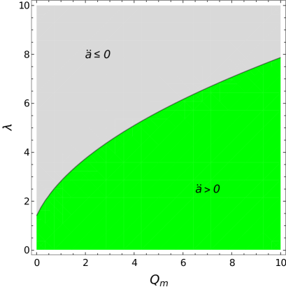
Figure 3: The region of parameters $\lambda$ and $Q_{m}$ allowing for acceleration at late times.

Note that the larger is $Q_{m}$, the easiest is to enter in the accelerating regime, with $x_{4}\to 0$ and $y_{4}\to 1$ for $Q_{m}\gg 1$ and $\lambda\ll 1$. Physically, the dissipation term $\Upsilon_{m}$ acts as a friction term slowing down the quintessence field at later times and making it easier to enter the accelerating regime $\ddot{a}>0$.

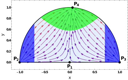
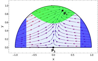
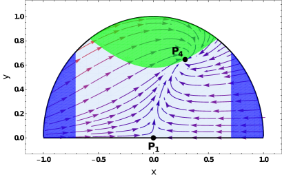
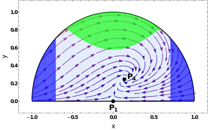
Figure 4: Snapshots of the phase space trajectories of the dynamical system in the plane $(x,y)$ for different values of parameters. Panel a: $Q_{m}=0$, $\lambda=\lambda_{\rm accel}/10$; Panel b: $Q_{m}=1$, $\lambda=\lambda_{\rm accel}/10$; Panel c: $Q_{m}=1$, $\lambda=\lambda_{\rm accel}/2$; Panel d: $Q_{m}=1$, $\lambda=\lambda_{\rm accel}$; Panel e: $Q_{m}=1$, $\lambda=3\lambda_{\rm accel}$.

The region in the parameters $Q_{m}$ and $\lambda$ for which the point $P_{4}$ is in the accelerating regime is illustrated in Fig. 3. Note that the larger values of $Q_{m}$ allow for steeper potentials to work as quintessence fields (i.e., allowing for later accelerated regimes). The boundary of the accelerating and nonaccelerating regions shown in Fig. 3 is given by the condition $x_{4}^{2}-y_{4}^{2}=-1/3$, i.e., where the equation of state is exactly $\omega=-1/3$. It is found to be given by

$$\lambda_{\rm accel}=\sqrt{2+6Q_{m}}.$$ (41)

In Fig. 4, we give snapshots of the phase space trajectories of the dynamical system in the plane $(x,y)$ for different values of parameters. The green shaded region denotes the accelerating region, the blue shaded region is the kination region, where the kinetic energy of the quintessence field dominates, and which satisfies $x^{2}>1/2$. The gray region is the matter dominated region.

Note that for $Q_{m}>0$, the points $P_{2}$ and $P_{3}$ move away from the boundary of the region shown in Fig. 4. This is why they are not shown in Fig. 4 panels (b)-(e). Since $P_{2}$ and $P_{3}$ lie in the kination regions, the trajectories then emanate from the blue region. Note also that as $\lambda$ increases (for a fixed value of $Q_{m}$), the point $P_{4}$ moves from the accelerating region and towards the point $P_{1}$ for matter domination. It is interesting to look at the corresponding value of $\lambda_{\rm accel}$ from the example given in Fig. 1. At later times, the total dissipation ratio $Q_{m}=Q_{m,1}+Q_{m,2}$ flattens with a value $Q_{m}\simeq 10^{4}$. From Eq. (41), the corresponding value for $\lambda_{\rm accel}$ is then $\lambda_{\rm accel}\sim 240$. The value of $\lambda$ at later times in the case of the initial conditions used in the example of Fig. 1 is $\lambda_{f}\sim 22\ll\lambda_{\rm accel}$. Thus, the system at later times goes to the accelerating dark energy dominated regime as expected.

V Late time dynamics: full dynamical system analysis

The quintessential scalar field predominantly dissipates to matter energy density during the late times as it is evident from Fig. 1. Therefore, for the late-time dynamics, one can ignore the contribution of the radiation bath ($\Omega_{r}\approx 0$), which means that we can also ignore the equations of $\Omega_{r}$ and $Q_{r}$ as given in Eqs. (16) and (26), respectively. Hence, the previous dynamical system of six equations now reduces to a dynamical system of four equations:

$$x^{\prime} = -\frac{3x(1-x^{2})}{2}-3xQ_{m}+\sqrt{\frac{3}{2}}\lambda y^{2}-\frac{3xy^{2}}{2},$$ (42)

$$y^{\prime} = \frac{3y}{2}+\frac{3x^{2}y}{2}-\frac{3y^{3}}{2}-\sqrt{\frac{3}{2}}xy\lambda,$$ (43)

$$Q_{m}^{\prime} = \frac{3(2-k)Q_{m}}{4}+\frac{3(x^{2}-y^{2})Q_{m}}{2}$$ (44)

$$\!\!\!\!+ \!\!\!\!\!\sqrt{6}qx\left(\frac{n\alpha}{\lambda}\right)^{\frac{1}{-1+n}}Q_{m}-\frac{3kx^{2}Q_{m}^{2}}{2\left(-1+x^{2}+y^{2}\right)},$$

$$\lambda^{\prime} = \sqrt{6}x(n-1)(\alpha n)^{\frac{1}{n-1}}\lambda^{\frac{n-2}{n-1}},$$ (45)

and the constraint equation given in Eq. (12) becomes

$$1=x^{2}+y^{2}+\Omega_{m}.$$ (46)

We define the equation of state of the total fluid (including both $\Omega_{m}$ and $\Omega_{\phi}$) as

$$\omega_{\rm tot}\equiv\frac{p_{\phi}+p_{m}}{\rho_{\phi}+\rho_{m}}=x^{2}-y^{2}.$$ (47)

Before analyzing the set of autonomous equations, we note that, though $x$ and $y$ are bounded between -1 to 1 by the constraint given in Eq. (46), $\lambda$ and $Q_{m}$ are unbounded and can take values between 0 to $\infty$. To obtain dynamical parameters which are bounded, unlike $\lambda$ and $Q_{m}$, it becomes convenient to introduce two new variables $z$ and $\xi$ that are defined as

$$z = \dfrac{\lambda^{\frac{1}{n-1}}}{1+\lambda^{\frac{1}{n-1}}},$$ (48)

$$\xi = \frac{Q_{m}}{1+Q_{m}},$$ (49)

which make $z$ and $\xi$ range from $0<z<1$ and $0<\xi<1$. However, we found that the transformed dynamical set of equations in terms of $(x,y,z,\xi)$ displays only the trivial critical point $(0,0,z,0)$, while the other possible critical points, including any accelerating solutions, remain hidden. This seems to be a drawback of the choice of variables made, but that can be overcame as follows. To work around the above mentioned difficulty, we first redefine $z$ as

$$z=\dfrac{1-\lambda^{\frac{1}{n-1}}}{\lambda^{\frac{1}{n-1}}},$$ (50)

which now ranges from $-1<z\leq 0$ for values $1\leq\lambda<\infty$. Here we note that for values of $\lambda$ smaller than unity, $z$ again becomes unbounded which we do not want. That is why we restrict the lower value of $\lambda$ to 1.

Next, we can make a nontrivial transformation of the variables $z$ and $\xi$ to two other parameters $u$ and $v$ as

$$u=\frac{\xi-z}{\xi+z},\quad v=\frac{\xi-z}{\xi^{2}}\,,$$ (51)

such that

$$\xi=\frac{2u}{(1+u)v},\quad z=\frac{2u(1-u)}{(1+u)^{2}v}.$$ (52)

The $\xi$ and $z$ variables ranges (which are, respectively, given by $0<\xi<1$ and $-1<z\leq 0$) put constraints on the $u$ and $v$ values as

$$u\leq-1\implies v>\frac{2(u-1)u}{(u+1)^{2}},$$

$$u\geq 1\implies v>\frac{2u}{u+1}.$$ (53)

Therefore, in terms of the four variables $(x,y,u,v)$, we get the set of autonomous equations as follows,

$$x^{\prime} = \frac{3y^{2}}{\sqrt{6}}\left(\frac{v(1+u)^{2}}{v(1+u)^{2}+2u(1-u)}\right)^{n-1}+\dfrac{3}{2}x\left(-2-\dfrac{4xu}{v(1+u)-2u}+1+x^{2}-y^{2}\right),$$ (54)

$$y^{\prime} = \dfrac{-xy\sqrt{6}}{2}\left(\frac{v(1+u)^{2}}{v(1+u)^{2}+2u(1-u)}\right)^{n-1}+\dfrac{3y}{2}\left(1+x^{2}-y^{2}\right),$$ (55)

$$u^{\prime} = \frac{1}{4}\bigg{[}\frac{3kx^{2}}{2\Omega_{m}}\frac{4u^{2}(1-u)}{v}+\frac{2u(1-u)}{v}((1+u)v-2u)\bigg{\{}\frac{-3k}{4}+\frac{q\sqrt{6}x(\alpha\ n)^{\frac{1}{n-1}}}{(1+u)^{2}v}\left((1+u)^{2}v+2u-2u^{2}\right)$$ (56)

$$+\frac{3}{2}\left(1+x^{2}-y^{2}\right)\bigg{\}}+\frac{\sqrt{6}x\left((1+u)^{2}v+2u(1-u)\right)^{2}(\alpha\ n)^{\frac{1}{n-1}}}{(1+u)v}\bigg{]},$$

$$v^{\prime} = \frac{3kx^{2}}{2\Omega_{m}}u+\frac{(v(1+u)-2u)}{2}\left[\dfrac{-3k}{4}+q\sqrt{6}x(\alpha\ n)^{\frac{1}{n-1}}\frac{\left((1+u)^{2}v+2u-2u^{2}\right)}{(1+u)^{2}v}+\frac{3}{2}\left(1+x^{2}-y^{2}\right)\right]$$ (57)

$$+\sqrt{6}x(\alpha\ n)^{\frac{1}{n-1}}\frac{\left((1+u)^{2}v+2u(1-u)\right)^{2}}{4u(1+u)^{2}}-\frac{6kx^{2}}{\Omega_{m}}\dfrac{u}{(1+u)}-\frac{2((1+u)v-2u)}{(1+u)}\bigg{[}-\frac{3k}{4}+q\sqrt{6}x(\alpha n)^{\frac{1}{n-1}}$$

$$\times\dfrac{\left((1+u)^{2}v+2u-2u^{2}\right)}{(1+u)^{2}v}+\frac{3}{2}\left(1+x^{2}-y^{2}\right)\bigg{]}\,,$$

where $\Omega_{m}=1-x^{2}-y^{2}$ from Eq. (46). It is to note that the dynamical system analysis with steeper exponential potentials ($n>1$) is a tasking job, as has been pointed out in Das:2019ixt . The linear stability analysis Bahamonde:2017ize breaks down in such cases as the real parts of some of the eigenvalues turn out to be zero. In Das:2019ixt , the authors used the center manifold theorem to analyze the stability of a system with steep exponential potentials. However, for the present problem we found that with dissipation of the scalar field to the matter sector, the system becomes too intricate to be analyzed employing the center manifold theorem technique. Therefore, we chose the non-trivial parametrization, given in Eq. (51), which enables us to do the stability analysis of the system with dissipation.

The non-trivial transformation in Eq. (51) has created a complicated structure of the autonomous system, making it difficult to identify the critical points analytically. Therefore, we shall compute the fixed points by assuming some representative values of the model parameters $(k,q,n,\alpha)$. The advantage of this non-trivial transformation is that we can find non-trivial fixed points and the linearization technique Bahamonde:2017ize does not break down, allowing us to find non-zero eigenvalues. We select the fixed points based on the constraints $0\leq x^{2}+y^{2}\leq 1$ and $0<\xi<1,\ -1<z\leq 0$.

Before we proceed to find the fixed points and their corresponding eigenvalues, we note that in Eqs. (56) and (57), the term $x^{2}/\Omega_{m}$ is discontinuous at the point $(x=0,y=1)$,

$$\lim_{\begin{subarray}{c}x\to 0\\ y\to 1\end{subarray}}\frac{x^{2}}{1-x^{2}-y^{2}}=0,\quad\lim_{\begin{subarray}{c}y\to 1\\ x\to 0\end{subarray}}\frac{x^{2}}{1-x^{2}-y^{2}}=-1.$$ (58)

However, this discontinuity can be removed by multiplying the above expression by $x$. Therefore, in the autonomous equations this can be achieved by redefining the time variable ${dN}\to x\ {dN}$. This redefinition does not change the dynamics of the system and it removes the discontinuity. Therefore, the structure of the new autonomous system becomes

$$\frac{d\vec{x}}{dN}=f(\vec{x})\times x,$$ (59)

where $\vec{x}=\{x,y,u,v\}$. This set of autonomous equations is now suitable for finding completely all the critical points. The critical points for four different example cases have been evaluated in Table 1. To determine the critical points and for illustration, we have fixed the parameters $n$ and $\alpha$ of the potential as $n=3$ and $\alpha=0.015$ as have been considered in Ref. Lima:2019yyv , while four different representative choices for $k$ and $q$ are made. The motivation for the choice of parameters come from the fact, as shown in Refs. Lima:2019yyv and Das:2020xmh , that the type of runaway exponential potential that we have studied here satisfies well the observations (e.g., the tensor-to-scalar ratio $r$ and spectral tilt $n_{s}$) for the cases for which the power $n$ in the potential is equal to or larger than 2. Hence, we have fixed in our examples the case $n=3$ as a representative case, ensuring that the warm inflationary dynamics can correctly satisfy the Planck results for $r$ and $n_{s}$. The same reason motivated our different choices for the constant $\alpha$ in the potential, while the choices for $k$ and $q$, that controls the dissipation in the dark energy regime, were chosen in analogy to the similar powers ($c$ and $p$) appearing in the dissipation coefficient during the inflationary regime. We discuss the stability of these four chosen cases below.

Points	$(x,y,u,v)$	$\omega_{\rm tot}$	$\Omega_{\phi}$	$\Omega_{m}$	Stability
Case I: $\bf n=3,\ k=3,\ q=-2,\ \alpha=0.015$
$M_{0}$	$(0,\ any,\ any,\ any)$	$-y^{2}$	$y^{2}$	$1-y^{2}$	Stable
$M_{1}$	$(-0.06,0.96,1.44,1.19)$	$-0.92$	$0.92$	$0.08$	Saddle
$M_{2}$	$(0.34,0.82,2.02,2.69)$	$-0.56$	$0.79$	$0.21$	Saddle
$M_{3}$	$(0.17,0.23,7.11,2.01)$	$-0.06$	$0.12$	$0.88$	Saddle
$M_{4}$	$(-0.16,0.04,3.59,1.93)$	$0.02$	$0.03$	$0.97$	Saddle
Case II: $\bf n=3,\ k=-1,\ q=0,\ \alpha=0.015$
$M_{0}$	$(0,\ any,\ any,\ any)$	$-y^{2}$	$y^{2}$	$1-y^{2}$	Stable
Case III: $\bf n=3,\ k=0,\ q=0,\alpha=0.001$
$M_{0}$	$(0.20,0.84,1.99,1.45)$	$-0.66$	$0.74$	$0.26$	Stable
$M_{1}$	$(0.39,0.87,1.99,4.33)$	$-0.60$	$0.91$	$0.09$	Saddle
Case IV: $\bf n=3,\ k=3,\ q=0,\alpha=0.015$
$M_{0}$	$(0,any,any,any)$	$-y^{2}$	$y^{2}$	$1-y^{2}$	Stable
$M_{1}$	$(0.38,0.86,1.99,3.32)$	$-0.59$	$0.88$	$0.12$	Saddle
$M_{2}$	$(0.09,0,1.99,1.66)$	$0.01$	$0.01$	$0.99$	Saddle

Table 1: Critical points of the redefined autonomous system.

V.1 Case I: $\ n=3,\ k=3,\ q=-2,\ \alpha=0.015$

Firstly, we consider the model with $k=3$ and $q=-2$, which corresponds to the dissipation coefficient $\Upsilon_{m,1}$ (and therefore $Q_{m,1}$) given in Eq. (28). According to Fig. 2, this dissipation coefficient is responsible for the decay of the quintessence field into matter during the early phases of the evolution. In this case, we found the five critical points as given in Table 1.

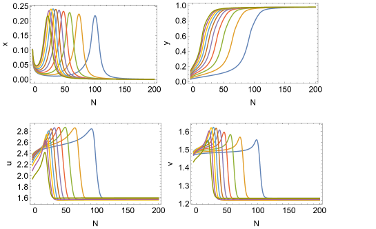
Figure 5: Numerical evolution of the autonomous equations for the critical point $M_{0}$ with $k=3,q=-2,n=3,\alpha=0.015$. The dynamical parameters $x$, $y$, $u$, and $v$ have been evolved numerically with ten different initial conditions. The ten different colored lines in each of these panels represent the evolution of these parameters with these varied initial conditions. The initial values of each of these parameters can be read from each of the plots at $N=0$.

The critical points $M_{1}$ and $M_{2}$ indicate accelerating solutions with equation of state given by $\omega_{\rm tot}=-0.92$ and $\omega_{\rm tot}=-0.56$, respectively. In these cases, the scalar field density dominates over the matter energy density. However, we found both these points to be saddles. The critical points $M_{3}$ and $M_{4}$ indicate matter domination, $\omega_{\rm tot}\sim 0$, with matter density dominating over the scalar field density. Both of these points turn out to be saddles too. At the fifth critical point, $M_{0}$, the eigenvalues turn out to be zero, the conventional linearization technique is no longer applicable. Hence, the stability for this critical point has to be determined numerically by varying the initial conditions. If $x=0$ initially, $(y,u,v)$ can take any value maintaining the constraint relations $0\leq x^{2}+y^{2}\leq 1$, $0<\xi<1$ and $-1<z\leq 0$. We then evolve the system numerically and the evolution of the dynamical parameters $(x,y,u,v)$ is depicted in the Fig. 5. We show in this figure that, even if we choose the initial values away from the critical point, they converge to $(x,y,u,v)\simeq(0,1,1.6,1.2)$ as time goes by, ensuring a stable solution at late times. We plot the evolution of the cosmological parameters $\omega_{\rm tot}$, $\Omega_{\phi}$ and $\Omega_{m}$ for this critical point in Fig. 6. It is seen that $\omega_{\rm tot}$ tends to $-1$ steadily at later times and the energy density is fully dominated by the scalar field density $\Omega_{\phi}$. Figures 5 and 6 confirm that the critical point $M_{0}$ is stable and yields an accelerating solution with $\omega_{\rm tot}\sim-1$.

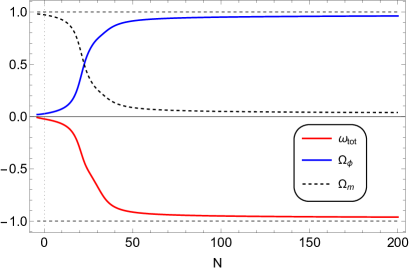
Figure 6: Evolution of cosmological parameters $(\omega_{\rm tot},\ \Omega_{\phi},\ \Omega_{m})$ corresponds to the critical point $M_{0}$ with $k=3,\ q=-2,\ n=3,\ \alpha=0.015$.

V.2 Case II: $n=3,\ k=-1,\ q=0,\ \alpha=0.015$

Here, we consider for illustration the model with $k=-1$ and $q=0$, which correspond to the dissipation coefficient $\Upsilon_{m,2}$ (and therefore $Q_{m,2}$) given in Eq. (29). According to Fig. 2, this dissipation coefficient is responsible for the decay of the quintessence field into matter during late times. We found only one critical point $M_{0}$ for this case. As before, the eigenvalues for this critical point turn out to be zero. Hence, we then resort again to a numerical analysis of the stability for this point. Initially, $(y,u,v)$ can take any value maintaining the constraint relations $0\leq x^{2}+y^{2}\leq 1$, $0<\xi<1$ and $-1<z\leq 0$, with fixed $x=0$. We evolve the system numerically and the corresponding evolution of the dynamical parameters $(x,y,u,v)$ is depicted in Fig. 7. We see that although $x,y$ and $v$ converge at late times, $u$ does not converge to a single value. Still, the system does not diverge and, thus, shows stability at late times. To establish the stability of this point, we further plot the evolution of the cosmological parameters $\omega_{\rm tot}$, $\Omega_{\phi}$ and $\Omega_{m}$ for this critical point in Fig. 8. We see from the result shown in that figure that $\omega_{\rm tot}$ steadily tends to -1 for any initial condition, with scalar field density dominating over matter energy density ($\Omega_{\phi}\sim 1$). Both figures 7 and 8 show that the critical point $M_{0}$ is stable and yields an accelerating solution with $\omega_{\rm tot}\sim-1$.

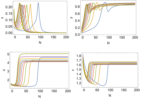
Figure 7: Numerical evolution of the autonomous equations for the critical point $M_{0}$ with $k=-1,q=0,n=3,\alpha=0.015$.The dynamical parameters $x$, $y$, $u$, and $v$ have been evolved numerically with ten different initial conditions. The ten different colored lines in each of these panels represent the evolution of these parameters with these varied initial conditions. The initial values of each of these parameters can be read from each of the plots at $N=0$.

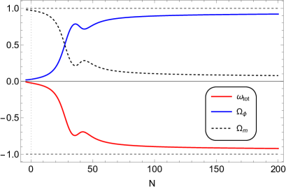
Figure 8: Evolution of cosmological parameters $(\omega_{\rm tot},\ \Omega_{\phi},\ \Omega_{m})$ corresponds to the critical point $M_{0}$ with $k=-1,\ q=0,\ n=3,\ \alpha=0.015$.

V.3 Case III: $n=3,\ k=0,\ q=0,\alpha=0.001$

Here, we consider the model with a constant dissipation, $\Upsilon_{m}=$ constant, which is obtained by setting $k=q=0$. Note that the $x^{2}/\Omega_{m}$ term, which leads to the discontinuity in Eq. (56) and Eq. (57), comes with the factor $k$. Thus, by setting $k=0$, we no longer face the discontinuity in the autonomous equations and Eqs. (54)–(57) yield the critical points for this case. We found no critical point for $\alpha=0.015$. However, after lowering the value to $\alpha$ to 0.001, we found two critical points, both of them indicating accelerating solutions. While $M_{1}$, with $\omega_{\rm tot}=-0.6$, is a saddle point, $M_{0}$ (with $\omega_{\rm tot}=-0.66$) turns out to be stable. We did not find any stable accelerating point with $\omega_{\rm tot}\sim-1$ for this case.

V.4 Case IV: $n=3,\ k=3,\ q=0,\alpha=0.015$

Finally, we consider the model with $k=3$ and $q=0$, which yields a dissipation coefficient like $\Upsilon_{m}\propto\rho_{m}^{3/4}$. We found three critical points for this case as shown in Table 1. The critical point $M_{1}$ shows accelerating characteristics, while $M_{2}$ produces non-accelerating behavior at which matter energy density dominates. Both $M_{1}$ and $M_{2}$ turn out to be saddle points. The critical point $M_{0}$ is studied numerically, like in the first two models. The stability of the system has been evaluated numerically in Fig. 9. We see that the parameters steadily converges to the values $(x,y,u,v)\simeq(0,1,1.6,1.2)$. We plot the evolution of the cosmological parameters $\omega_{\rm tot}$, $\Omega_{\phi}$ and $\Omega_{m}$ for this critical point in Fig. 10, which shows that the model can produce a stable accelerating solution with $\omega_{\rm tot}\sim-1$.

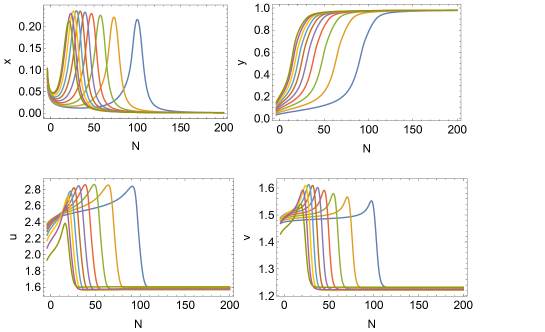
Figure 9: Numerical evolution of the autonomous equations for the critical point $M_{0}$ with $k=3,q=0,n=3,\alpha=0.015$. The dynamical parameters $x$, $y$, $u$, and $v$ have been evolved numerically with ten different initial conditions. The ten different colored lines in each of these panels represent the evolution of these parameters with these varied initial conditions. The initial values of each of these parameters can be read from each of the plots at $N=0$.

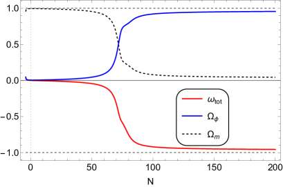
Figure 10: Evolution of cosmological parameters $(\omega_{\rm tot},\ \Omega_{\phi},\ \Omega_{m})$ corresponds to the critical point $M_{0}$ with $k=3,\ q=0,\ n=3,\ \alpha=0.015$.

VI Discussion and Conclusion

In this paper, we have studied a phenomenological model for quintessential inflation that is motivated from warm inflation. At early times, the quintessential scalar inflaton field decays into radiation during warm inflation, while at late times it is allowed to decay into matter, thus realizing a model of dissipative interaction in the dark sector at late times. The construction also makes use of a generalized exponential potential able to realize both phases of accelerated expansion, at early- and late-times. The full dynamical system was analyzed, with a focus on the behavior of the dynamical system at late times. The analysis was exemplified by both analytical and numerical results and for different illustrative values of parameters. The analysis performed here extents and generalizes the results originally obtained in Ref. Lima:2019yyv , where a version of this model was first proposed. The results obtained demonstrate the viability of the model as a quintessential inflation model and in which stable solutions can be obtained. In addition, we have also analyzed the stability of the slow-roll solutions at both early- and late-times, which allowed us to put some constraints in the model parameters.

Appendix A Slow-roll analysis of the dynamical system

In this section, we shall consider the stability of the slow-roll approximated dynamical system of the Warm Quintessential Dark Energy Model following Moss:2008yb . From the set of equations (1), (2) and (3), we see that there are three dynamical quantities $\phi$, $\rho_{r}$ and $\rho_{m}$. We express the radiation energy density $\rho_{r}$ in terms of the entropy density $s$ as $\rho_{r}=(3/4)sT$ and, thus, the above set of equations become

$$\ddot{\phi}+3H(1+Q_{r}+Q_{m})\dot{\phi}+V,_{\phi}=0,$$

$$T\dot{s}+3HTs=3HQ_{r}\dot{\phi}^{2},$$

$$\dot{\rho}_{m}+3H\rho_{m}=3HQ_{m}\dot{\phi}^{2}.$$ (60)

Under the slow-roll conditions, this set of background equations then reduce to

$$3H(1+Q_{r}+Q_{m})\dot{\phi}+V,_{\phi}=0,$$

$$Ts=Q_{r}\dot{\phi}^{2},$$

$$\rho_{m}=Q_{m}\dot{\phi}^{2}.$$ (61)

The leading order slow-roll parameters in this model are Moss:2008yb

$$\epsilon = \frac{1}{16\pi G}\left(\frac{V,_{\phi}}{V}\right)^{2},$$

$$\eta = \frac{1}{8\pi G}\frac{V,_{\phi\phi}}{V},$$

$$\kappa = \frac{1}{8\pi G}\frac{V,_{\phi}}{\phi V},$$

$$\beta = \frac{1}{8\pi G}\frac{V,_{\phi}\Gamma_{r},_{\phi}}{V\Gamma_{r}}=p\kappa,$$

$$\gamma = \frac{1}{8\pi G}\frac{V,_{\phi}\Gamma_{m},_{\phi}}{V\Gamma_{m}}=q\kappa,$$

$$\delta = \frac{TV,_{\phi T}}{V,_{\phi}}.$$ (62)

Here, we have defined an extra slow-roll parameter $\gamma$ in connection with the dissipation to the matter energy density, which is in general not present in standard WI models.

We find it convenient to change the independent variable from cosmic time $t$ to the inflaton field $\phi$ as a clock in the equations of motion. We also define $u\equiv\dot{\phi}$ and, thus, $\frac{d}{dt}=u\frac{d}{d\phi}$. Note that this variable $u$ is different from the dynamical variable $u$ we defined previously in Eq. (51). We also redefine $\rho_{m}\equiv w$. Then, the set of equations given in Eq. (60) can be written as

$$u^{\prime}=-3H-\Gamma_{r}-\Gamma_{m}-V,_{\phi}u^{-1}\equiv f(u,s,w),$$

$$s^{\prime}=-3Hsu^{-1}+T^{-1}\Gamma_{r}u\equiv g(u,s,w),$$

$$w^{\prime}=-3Hwu^{-1}+\Gamma_{u}u\equiv h(u,s,w),$$ (63)

where prime denotes derivative w.r.t. $\phi$. Therefore, the background set of equations can be compactly written as

$$x^{\prime}=F(x),$$ (64)

where

$$x\equiv\left(\begin{array}[]{c}u\\ s\\ w\end{array}\right).$$ (68)

We take a background $\bar{x}$, which satisfies the slow-roll equations, Eq. (61). Then, the linearized perturbations satisfy the equations

$$\delta x^{\prime}=M(\bar{x})\delta x-\bar{x},$$ (69)

where the $M$ matrix is defined as

$$M=\left.\frac{\partial(f,g,h)}{\partial(u,s,w)}\right|_{u=\bar{u},s=\bar{s},w=\bar{w}}.$$ (70)

We find the matrix elements as

$$\frac{\partial f}{\partial u}=\frac{H}{u}\left[-3(1+Q_{r}+Q_{m})-\frac{\epsilon}{(1+Q_{r}+Q_{m})^{2}}\right]\equiv\mathcal{A},$$

$$\frac{\partial f}{\partial s}=\frac{H}{s}\left[-cQ_{r}-\frac{Q_{r}\epsilon}{(1+Q_{r}+Q_{m})^{2}}\right.$$

$$\left.\;\;\;\;\;\;\;\;+\delta(1+Q_{r}+Q_{m})\frac{}{}\right]\equiv\mathcal{B},$$

$$\frac{\partial f}{\partial w}=\frac{H}{w}\left[-\frac{3k}{4}Q_{m}-\frac{Q_{m}\epsilon}{(1+Q_{r}+Q_{m})^{2}}\right]\equiv\mathcal{E},$$

$$\frac{\partial g}{\partial u}=\frac{Hs}{u^{2}}\left[6-\frac{\epsilon}{(1+Q_{r}+Q_{m})^{2}}\right]\equiv{\mathcal{C}},$$

$$\frac{\partial g}{\partial s}=\frac{H}{u}\left[c-4-\frac{Q_{r}\epsilon}{(1+Q_{r}+Q_{m})^{2}}\right]\equiv{\mathcal{D}},$$

$$\frac{\partial g}{\partial w}=\frac{Hs}{uw}\left[-\frac{Q_{m}\epsilon}{(1+Q_{r}+Q_{m})^{2}}\right]\equiv{\mathcal{F}},$$

$$\frac{\partial h}{\partial u}=\frac{Hw}{u^{2}}\left[6-\frac{\epsilon}{(1+Q_{r}+Q_{m})^{2}}\right]\equiv{\mathcal{G}},$$

$$\frac{\partial h}{\partial s}=\frac{Hw}{su}\left[-\frac{Q_{r}\epsilon}{(1+Q_{r}+Q_{m})^{2}}\right]\equiv{\mathcal{H}},$$

$$\frac{\partial h}{\partial w}=\frac{H}{u}\left[-3+\frac{3k}{4}-\frac{Q_{m}\epsilon}{(1+Q_{r}+Q_{m})^{2}}\right]\equiv{\mathcal{I}}.$$ (71)

The matrix $M$ can then be read as

$$M=\left(\begin{array}[]{ccccccc}{\mathcal{A}}&&\mathcal{B}&&{\mathcal{E}}\\ {\mathcal{C}}&&{\mathcal{D}}&&{\mathcal{F}}\\ {\mathcal{G}}&&{\mathcal{H}}&&{\mathcal{I}}\end{array}\right).$$ (75)

The sufficient condition for stability of this slow-roll approximated system is that the $M$ matrix varies slowly, which is justified by having all the three eigenvalues of the diagonalized matrix to be negative. If all the three eigenvalues of the diagonalized matrix are negative, then both $\det(M)$ and ${\rm tr}(M)$ should be negative as well. We find, at leading order (ignoring slow-roll parameters),

$${\rm det}(M) = \frac{9}{4}\left((c-4)(4-k)+(c-4)(4+k)Q_{m}\right.$$

$$\left.+(c+4)(k-4)Q_{r}\right),$$

$${\rm tr}(M) = -7+c+\frac{3k}{4}-3(1+Q_{m}+Q_{r}).$$ (76)

Thus, to have $\det(M)$ negative, we find the conditions $-4<c<4$ and $-4<k<4$. These conditions also make ${\rm tr}(M)$ negative. We can see it explicitly that these conditions yield three negative eigenvalues of the matrix $M$ in three different physical situations:

1. Strong dissipative inflationary regime ($Q_{r}\gg 1$ and $Q_{m}\ll 1$): During slow-roll, with these limits, we find three eigenvalues of the matrix $M$ as $\lambda_{1}=(3/4)(-4+k)$, $\lambda_{2}=2c-3Q_{r}$ and $\lambda_{3}=-4-c$. We note that the three eigenvalues can be simultaneously negative only if $-4<c<4$ and $-4<k<4$.

2. Weak dissipative inflationary regime ($Q_{r}\ll 1$ and $Q_{m}\ll 1$): In this case, we find the three eigenvalues as $\lambda_{1}=-3$, $\lambda_{2}=-4+c$ and $\lambda_{3}=(3/4)(-4+k)$. Here also, we note that the conditions to get all the three eigenvalues negative are $-4<c<4$ and $-4<k<4$.

3. Quintessence driven Dark Energy dominated regime ($Q_{r}\ll 1$ and $Q_{m}\gg 1$): Here the three eigenvalues turn out to be $\lambda_{1}=-4+c$, $\lambda_{2}=(3/2)(k-2Q_{m})$ and $\lambda_{3}=-(3/4)(4+k)$. Like in the previous two cases, in this case too, the conditions to get all the three eigenvalues negative are $-4<c<4$ and $-4<k<4$.

Therefore, we see that for the system to be stabilized, the form of the dissipative coefficients $\Upsilon_{r}$ and $\Upsilon_{m}$ must involve the powers $c$ and $k$ satisfying the conditions $-4<c<4$ and $-4<k<4$.

- (1) D. Kazanas, “Dynamics of the Universe and Spontaneous Symmetry Breaking,” Astrophys. J. Lett. 241, L59-L63 (1980) doi:10.1086/183361
- (2) A. H. Guth, The Inflationary Universe: A Possible Solution to the Horizon and Flatness Problems, Phys. Rev. D 23, 347-356 (1981) doi:10.1103/PhysRevD.23.347
- (3) K. Sato, Cosmological Baryon Number Domain Structure and the First Order Phase Transition of a Vacuum, Phys. Lett. B 99, 66-70 (1981) doi:10.1016/0370-2693(81)90805-4
- (4) K. Sato, “First Order Phase Transition of a Vacuum and Expansion of the Universe,” Mon. Not. Roy. Astron. Soc. 195, 467-479 (1981) NORDITA-80-29.
- (5) A. D. Linde, A New Inflationary Universe Scenario: A Possible Solution of the Horizon, Flatness, Homogeneity, Isotropy and Primordial Monopole Problems, Phys. Lett. B 108, 389-393 (1982) doi:10.1016/0370-2693(82)91219-9
- (6) A. Albrecht and P. J. Steinhardt, Cosmology for Grand Unified Theories with Radiatively Induced Symmetry Breaking, Phys. Rev. Lett. 48, 1220-1223 (1982) doi:10.1103/PhysRevLett.48.1220
- (7) S. Perlmutter et al. [Supernova Cosmology Project], Measurements of and from 42 high redshift supernovae, Astrophys. J. 517, 565-586 (1999) doi:10.1086/307221 [arXiv:astro-ph/9812133 [astro-ph]].
- (8) A. G. Riess et al. [Supernova Search Team], Observational evidence from supernovae for an accelerating universe and a cosmological constant, Astron. J. 116, 1009-1038 (1998) doi:10.1086/300499 [arXiv:astro-ph/9805201 [astro-ph]].
- (9) P. J. E. Peebles and B. Ratra, “Cosmology with a Time Variable Cosmological Constant,” Astrophys. J. Lett. 325, L17 (1988) doi:10.1086/185100
- (10) B. Ratra and P. J. E. Peebles, “Cosmological Consequences of a Rolling Homogeneous Scalar Field,” Phys. Rev. D 37, 3406 (1988) doi:10.1103/PhysRevD.37.3406
- (11) K. Bamba, S. Capozziello, S. Nojiri and S. D. Odintsov, Dark energy cosmology: the equivalent description via different theoretical models and cosmography tests, Astrophys. Space Sci. 342, 155-228 (2012) doi:10.1007/s10509-012-1181-8 [arXiv:1205.3421 [gr-qc]].
- (12) S. Tsujikawa, Quintessence: A Review, Class. Quant. Grav. 30, 214003 (2013) doi:10.1088/0264-9381/30/21/214003 [arXiv:1304.1961 [gr-qc]].
- (13) J. de Haro and L. A. Saló, A Review of Quintessential Inflation, Galaxies 9, no.4, 73 (2021) doi:10.3390/galaxies9040073 [arXiv:2108.11144 [gr-qc]].
- (14) D. Bettoni and J. Rubio, “Quintessential Inflation: A Tale of Emergent and Broken Symmetries,” Galaxies 10, no.1, 22 (2022) doi:10.3390/galaxies10010022 [arXiv:2112.11948 [astro-ph.CO]].
- (15) L. H. Ford, Gravitational Particle Creation and Inflation, Phys. Rev. D 35, 2955 (1987) doi:10.1103/PhysRevD.35.2955
- (16) E. J. Chun, S. Scopel and I. Zaballa, Gravitational reheating in quintessential inflation, JCAP 07, 022 (2009) doi:10.1088/1475-7516/2009/07/022 [arXiv:0904.0675 [hep-ph]].
- (17) G. N. Felder, L. Kofman and A. D. Linde, Instant preheating, Phys. Rev. D 59, 123523 (1999) doi:10.1103/PhysRevD.59.123523 [arXiv:hep-ph/9812289 [hep-ph]].
- (18) A. H. Campos, H. C. Reis and R. Rosenfeld, Preheating in quintessential inflation, Phys. Lett. B 575, 151-156 (2003) doi:10.1016/j.physletb.2003.09.064 [arXiv:hep-ph/0210152 [hep-ph]].
- (19) B. Feng and M. z. Li, Curvaton reheating in nonoscillatory inflationary models, Phys. Lett. B 564, 169-174 (2003) doi:10.1016/S0370-2693(03)00589-6 [arXiv:hep-ph/0212213 [hep-ph]].
- (20) J. C. Bueno Sanchez and K. Dimopoulos, Curvaton reheating allows TeV Hubble scale in NO inflation, JCAP 11, 007 (2007) doi:10.1088/1475-7516/2007/11/007 [arXiv:0707.3967 [hep-ph]].
- (21) K. Dimopoulos and T. Markkanen, Non-minimal gravitational reheating during kination, JCAP 06, 021 (2018) doi:10.1088/1475-7516/2018/06/021 [arXiv:1803.07399 [gr-qc]].
- (22) D. Bettoni and J. Rubio, Phys. Lett. B 784, 122-129 (2018) doi:10.1016/j.physletb.2018.07.046 [arXiv:1805.02669 [astro-ph.CO]].
- (23) T. Opferkuch, P. Schwaller and B. A. Stefanek, Ricci Reheating, JCAP 07, 016 (2019) doi:10.1088/1475-7516/2019/07/016 [arXiv:1905.06823 [gr-qc]].
- (24) A. Berera, Warm inflation, Phys. Rev. Lett. 75, 3218-3221 (1995) doi:10.1103/PhysRevLett.75.3218 [arXiv:astro-ph/9509049 [astro-ph]].
- (25) V. Kamali, M. Motaharfar and R. O. Ramos, Recent Developments in Warm Inflation, Universe 9, no.3, 124 (2023) doi:10.3390/universe9030124 [arXiv:2302.02827 [hep-ph]].
- (26) A. Berera, The warm inflation story, [arXiv:2305.10879 [hep-ph]].
- (27) H. Ooguri, E. Palti, G. Shiu and C. Vafa, Distance and de Sitter Conjectures on the Swampland, Phys. Lett. B 788, 180-184 (2019) doi:10.1016/j.physletb.2018.11.018 [arXiv:1810.05506 [hep-th]].
- (28) S. K. Garg and C. Krishnan, Bounds on Slow Roll and the de Sitter Swampland, JHEP 11, 075 (2019) doi:10.1007/JHEP11(2019)075 [arXiv:1807.05193 [hep-th]].
- (29) P. Agrawal, G. Obied, P. J. Steinhardt and C. Vafa, On the Cosmological Implications of the String Swampland, Phys. Lett. B 784, 271-276 (2018) doi:10.1016/j.physletb.2018.07.040 [arXiv:1806.09718 [hep-th]].
- (30) W. H. Kinney, S. Vagnozzi and L. Visinelli, Class. Quant. Grav. 36, no.11, 117001 (2019) doi:10.1088/1361-6382/ab1d87 [arXiv:1808.06424 [astro-ph.CO]].
- (31) S. Das, Note on single-field inflation and the swampland criteria, Phys. Rev. D 99, no.8, 083510 (2019) doi:10.1103/PhysRevD.99.083510 [arXiv:1809.03962 [hep-th]].
- (32) M. Motaharfar, V. Kamali and R. O. Ramos, Warm inflation as a way out of the swampland, Phys. Rev. D 99, no.6, 063513 (2019) doi:10.1103/PhysRevD.99.063513 [arXiv:1810.02816 [astro-ph.CO]].
- (33) S. Das, Warm Inflation in the light of Swampland Criteria, Phys. Rev. D 99, no.6, 063514 (2019) doi:10.1103/PhysRevD.99.063514 [arXiv:1810.05038 [hep-th]].
- (34) A. Berera and J. Calderón-Figueroa, Looking inside the Swampland from Warm Inflation: Dissipative Effects in De Sitter Expansion, Universe 9, no.4, 168 (2023) doi:10.3390/universe9040168
- (35) E. Ó. Colgáin and H. Yavartanoo, Phys. Lett. B 797, 134907 (2019) doi:10.1016/j.physletb.2019.134907 [arXiv:1905.02555 [astro-ph.CO]].
- (36) A. Banerjee, H. Cai, L. Heisenberg, E. Ó. Colgáin, M. M. Sheikh-Jabbari and T. Yang, Phys. Rev. D 103, no.8, L081305 (2021) doi:10.1103/PhysRevD.103.L081305 [arXiv:2006.00244 [astro-ph.CO]].
- (37) N. Aghanim et al. [Planck], Astron. Astrophys. 641, A6 (2020) [erratum: Astron. Astrophys. 652, C4 (2021)] doi:10.1051/0004-6361/201833910 [arXiv:1807.06209 [astro-ph.CO]].
- (38) A. G. Riess, L. M. Macri, S. L. Hoffmann, D. Scolnic, S. Casertano, A. V. Filippenko, B. E. Tucker, M. J. Reid, D. O. Jones and J. M. Silverman, et al. Astrophys. J. 826, no.1, 56 (2016) doi:10.3847/0004-637X/826/1/56 [arXiv:1604.01424 [astro-ph.CO]].
- (39) A. G. Riess, S. Casertano, W. Yuan, L. Macri, B. Bucciarelli, M. G. Lattanzi, J. W. MacKenty, J. B. Bowers, W. Zheng and A. V. Filippenko, et al. Astrophys. J. 861, no.2, 126 (2018) doi:10.3847/1538-4357/aac82e [arXiv:1804.10655 [astro-ph.CO]].
- (40) A. G. Riess, S. Casertano, W. Yuan, L. M. Macri and D. Scolnic, Astrophys. J. 876, no.1, 85 (2019) doi:10.3847/1538-4357/ab1422 [arXiv:1903.07603 [astro-ph.CO]].
- (41) A. Domínguez, R. Wojtak, J. Finke, M. Ajello, K. Helgason, F. Prada, A. Desai, V. Paliya, L. Marcotulli and D. Hartmann, doi:10.3847/1538-4357/ab4a0e [arXiv:1903.12097 [astro-ph.CO]].
- (42) C. G. Park and B. Ratra, Phys. Rev. D 101, no.8, 083508 (2020) doi:10.1103/PhysRevD.101.083508 [arXiv:1908.08477 [astro-ph.CO]].
- (43) W. Lin and M. Ishak, JCAP 05, 009 (2021) doi:10.1088/1475-7516/2021/05/009 [arXiv:1909.10991 [astro-ph.CO]].
- (44) W. L. Freedman, B. F. Madore, T. Hoyt, I. S. Jang, R. Beaton, M. G. Lee, A. Monson, J. Neeley and J. Rich, doi:10.3847/1538-4357/ab7339 [arXiv:2002.01550 [astro-ph.GA]].
- (45) S. Birrer, A. J. Shajib, A. Galan, M. Millon, T. Treu, A. Agnello, M. Auger, G. C. F. Chen, L. Christensen and T. Collett, et al. Astron. Astrophys. 643, A165 (2020) doi:10.1051/0004-6361/202038861 [arXiv:2007.02941 [astro-ph.CO]].
- (46) S. S. Boruah, M. J. Hudson and G. Lavaux, Mon. Not. Roy. Astron. Soc. 507, no.2, 2697-2713 (2021) doi:10.1093/mnras/stab2320 [arXiv:2010.01119 [astro-ph.CO]].
- (47) W. L. Freedman, Astrophys. J. 919, no.1, 16 (2021) doi:10.3847/1538-4357/ac0e95 [arXiv:2106.15656 [astro-ph.CO]].
- (48) Q. Wu, G. Q. Zhang and F. Y. Wang, Mon. Not. Roy. Astron. Soc. 515, no.1, L1-L5 (2022) doi:10.1093/mnrasl/slac022 [arXiv:2108.00581 [astro-ph.CO]].
- (49) S. Cao and B. Ratra, Mon. Not. Roy. Astron. Soc. 513, no.4, 5686-5700 (2022) doi:10.1093/mnras/stac1184 [arXiv:2203.10825 [astro-ph.CO]].
- (50) K. Dimopoulos and L. Donaldson-Wood, Warm quintessential inflation, Phys. Lett. B 796, 26-31 (2019) doi:10.1016/j.physletb.2019.07.017 [arXiv:1906.09648 [gr-qc]].
- (51) J. G. Rosa and L. B. Ventura, Warm Little Inflaton becomes Dark Energy, Phys. Lett. B 798, 134984 (2019) doi:10.1016/j.physletb.2019.134984 [arXiv:1906.11835 [hep-ph]].
- (52) G. B. F. Lima and R. O. Ramos, Unified early and late Universe cosmology through dissipative effects in steep quintessential inflation potential models, Phys. Rev. D 100, no.12, 123529 (2019) doi:10.1103/PhysRevD.100.123529 [arXiv:1910.05185 [astro-ph.CO]].
- (53) R. D’Agostino and O. Luongo, “Cosmological viability of a double field unified model from warm inflation,” Phys. Lett. B 829, 137070 (2022) doi:10.1016/j.physletb.2022.137070 [arXiv:2112.12816 [astro-ph.CO]].
- (54) H. P. de Oliveira and R. O. Ramos, Dynamical system analysis for inflation with dissipation, Phys. Rev. D 57, 741-749 (1998) doi:10.1103/PhysRevD.57.741 [arXiv:gr-qc/9710093 [gr-qc]].
- (55) I. G. Moss and C. Xiong, On the consistency of warm inflation, JCAP 11, 023 (2008) doi:10.1088/1475-7516/2008/11/023 [arXiv:0808.0261 [astro-ph]].
- (56) S. del Campo, R. Herrera, D. Pavón and J. R. Villanueva, On the consistency of warm inflation in the presence of viscosity, JCAP 08, 002 (2010) doi:10.1088/1475-7516/2010/08/002 [arXiv:1007.0103 [astro-ph.CO]].
- (57) M. Bastero-Gil, A. Berera, R. Cerezo, R. O. Ramos and G. S. Vicente, Stability analysis for the background equations for inflation with dissipation and in a viscous radiation bath, JCAP 11, 042 (2012) doi:10.1088/1475-7516/2012/11/042 [arXiv:1209.0712 [astro-ph.CO]].
- (58) X. B. Li, Y. Y. Wang, H. Wang and J. Y. Zhu, Phys. Rev. D 98, no.4, 043510 (2018) doi:10.1103/PhysRevD.98.043510 [arXiv:1804.05360 [gr-qc]].
- (59) Y. L. Bolotin, A. Kostenko, O. A. Lemets and D. A. Yerokhin, Cosmological Evolution With Interaction Between Dark Energy And Dark Matter, Int. J. Mod. Phys. D 24, no.03, 1530007 (2014) doi:10.1142/S0218271815300074 [arXiv:1310.0085 [astro-ph.CO]].
- (60) B. Wang, E. Abdalla, F. Atrio-Barandela and D. Pavon, Dark Matter and Dark Energy Interactions: Theoretical Challenges, Cosmological Implications and Observational Signatures, Rept. Prog. Phys. 79, no.9, 096901 (2016) doi:10.1088/0034-4885/79/9/096901 [arXiv:1603.08299 [astro-ph.CO]].
- (61) L. Amendola, Coupled quintessence, Phys. Rev. D 62, 043511 (2000) doi:10.1103/PhysRevD.62.043511 [arXiv:astro-ph/9908023 [astro-ph]].
- (62) S. Bahamonde, C. G. Böhmer, S. Carloni, E. J. Copeland, W. Fang and N. Tamanini, Dynamical systems applied to cosmology: dark energy and modified gravity, Phys. Rept. 775-777, 1-122 (2018) doi:10.1016/j.physrep.2018.09.001 [arXiv:1712.03107 [gr-qc]].
- (63) C. Q. Geng, M. W. Hossain, R. Myrzakulov, M. Sami and E. N. Saridakis, Quintessential inflation with canonical and noncanonical scalar fields and Planck 2015 results, Phys. Rev. D 92, no.2, 023522 (2015) doi:10.1103/PhysRevD.92.023522 [arXiv:1502.03597 [gr-qc]].
- (64) C. Q. Geng, C. C. Lee, M. Sami, E. N. Saridakis and A. A. Starobinsky, Observational constraints on successful model of quintessential Inflation, JCAP 06, 011 (2017) doi:10.1088/1475-7516/2017/06/011 [arXiv:1705.01329 [gr-qc]].
- (65) S. Ahmad, R. Myrzakulov and M. Sami, Relic gravitational waves from Quintessential Inflation, Phys. Rev. D 96, no.6, 063515 (2017) doi:10.1103/PhysRevD.96.063515 [arXiv:1705.02133 [gr-qc]].
- (66) M. Shahalam, W. Yang, R. Myrzakulov and A. Wang, Late-time acceleration with steep exponential potentials, Eur. Phys. J. C 77, no.12, 894 (2017) doi:10.1140/epjc/s10052-017-5468-3 [arXiv:1802.00326 [gr-qc]].
- (67) S. Das, M. Banerjee and N. Roy, Dynamical System Analysis for Steep Potentials, JCAP 08, 024 (2019) doi:10.1088/1475-7516/2019/08/024 [arXiv:1903.02288 [gr-qc]].
- (68) M. R. Gangopadhyay, S. Myrzakul, M. Sami and M. K. Sharma, Paradigm of warm quintessential inflation and production of relic gravity waves, Phys. Rev. D 103, no.4, 043505 (2021) doi:10.1103/PhysRevD.103.043505 [arXiv:2011.09155 [astro-ph.CO]].
- (69) S. Basak, S. Bhattacharya, M. R. Gangopadhyay, N. Jaman, R. Rangarajan and M. Sami, The paradigm of warm quintessential inflation and spontaneous baryogenesis, JCAP 03, no.03, 063 (2022) doi:10.1088/1475-7516/2022/03/063 [arXiv:2110.00607 [astro-ph.CO]].
- (70) S. Das and R. O. Ramos, Runaway potentials in warm inflation satisfying the swampland conjectures, Phys. Rev. D 102, no.10, 103522 (2020) doi:10.1103/PhysRevD.102.103522 [arXiv:2007.15268 [hep-th]].
- (71) S. Das and R. O. Ramos, Running and Running of the Running of the Scalar Spectral Index in Warm Inflation, Universe 9, no.2, 76 (2023) doi:10.3390/universe9020076 [arXiv:2212.13914 [astro-ph.CO]].