A Simple Data Augmentation for Feature Distribution Skewed Federated Learning

Abstract

Federated learning (FL) facilitates collaborative learning among multiple clients in a distributed manner, while ensuring privacy protection. However, its performance is inevitably degraded as suffering data heterogeneity, i.e., non-IID data. In this paper, we focus on the feature distribution skewed FL scenario, which is widespread in real-world applications. The main challenge lies in the feature shift caused by the different underlying distributions of local datasets. While the previous attempts achieved progress, few studies pay attention to the data itself, the root of this issue. Therefore, the primary goal of this paper is to develop a general data augmentation technique at the input level, to mitigate the feature shift. To achieve this goal, we propose FedRDN, a simple yet remarkably effective data augmentation method for feature distribution skewed FL, which randomly injects the statistics of the dataset from the entire federation into the client’s data. By this, our method can effectively improve the generalization of features, thereby mitigating the feature shift. Moreover, FedRDN is a plug-and-play component, which can be seamlessly integrated into the data augmentation flow with only a few lines of code. Extensive experiments on several datasets show that the performance of various representative FL works can be further improved by combining them with FedRDN, which demonstrates the strong scalability and generalizability of FedRDN. The source code will be released.

1 Introduction

Federated learning [16] (FL) has been a de facto solution for distributed learning from discrete data among different edge devices like mobile phones, which has attracted wide attention involving various communities [25, 11, 3, 2]. It utilizes a credible server to communicate the privacy irrelevant information, e.g., model parameters, thereby collaboratively training the model on multiple distributed data clients, while the local data of each client is invisible to others. Such a design is simple yet can achieve superior performance. However, it is inevitable to suffer data heterogeneity when we deploy FL in real-world applications, which will greatly degrade the performance of FL [7, 17, 21].

Since data heterogeneity is widely common in many real-world cases, many researchers try to address this issue to improve the practicability of FL [7, 17, 5, 26]. However, most of them try to design a robust FL method that can handle different data heterogeneity settings. In fact, this is suboptimal since the discrepancy between different data heterogeneity settings like feature distribution skew and label distribution skew [14]. Hence, some studies try to design special FL algorithms for different settings [35, 37]. In this work, we focus on solving the feature distribution skew problem, a typical data statistical heterogeneity scenario in FL, as the data from discrete clients are always collected from different devices or environments, incurring different underlying distributions among clients’ data. In FL, the client-side only trains the data on its skewed data, resulting in significant local model bias, and a typical manifestation is inconsistent feature distribution across different clients, namely feature shift [18, 37]. To address this problem, FedBN [18] learns the client-specific batch normalization layer parameters for each client instead of learning only a single global model. HarmoFL [6] utilizes the potential knowledge of medical images in the frequency domain to mitigate the feature shift.

While the feature distribution skew has been explored in FL, little attention is paid to the data itself, especially the data augmentation. In FL, the common practice [6, 37, 18] is to integrate some normal operations in centralized learning in the data augmentation flow (e.g., transforms.Compose() in Pytorch) of each client like horizontal and vertical flips. This overlooks the effectiveness of data augmentation at the input level, i.e., data augmentation flow, even though it has shown effectiveness and generalizability in centralized learning, which leaves an alternative space to explore. Considering the root cause of this problem lies in the divergence of data distributions, we ask two questions: 1) why not proactively resolve it by directly addressing the data? 2) can we design an FL-specific data augmentation operation that can be integrated into the data augmentation flow? To answer these, we try to design a plug-and-play input-level data augmentation technique.

Although it may appear straightforward, effectively implementing data augmentation in federated learning poses a significant challenge due to the lack of direct access to the external data of other users. The main challenge lies in how to inject global information into augmented samples, thereby mitigating the distribution bias between different local datasets. To address this, FedMix [31] extends MIXUP to federated learning for label distribution skew by incorporating the mixing of averaged data across multiple clients. However, it is only suitable for the classification task and has not yet demonstrated the effectiveness of addressing feature distribution skew. Furthermore, permitting the exchange of averaged data introduces certain privacy concerns and risks. As for the data augmentation for feature distribution skew, FedFA [37] mitigates the feature shift through feature augmentation based on the statistics of latent features. The approach applies augmentation at the feature level, which lacks versatility and cannot be seamlessly integrated into a comprehensive data augmentation pipeline.

In this work, we propose a novel federated data augmentation technique, called FedRDN. We argue that the local bias is rooted in the model trains on the limited and skewed distribution. In centralized learning, we can collect as many different distributions of data to learn generalized feature representations. This motivates us to augment the data to different underlying distributions, indirectly reducing the difference in their distributions. To achieve this, FedRDN extends the standard data normalization to FL by randomly injecting statistics of local datasets into augmented samples, which is based on the insight that statistics of data are the essential characteristic of data distribution. It enables clients to access a wider range distribution of data, thereby enhancing the generalizability of features.

FedRDN is a remarkably simple yet surprisingly effective method. It is a non-parametric approach that incurs minimal additional computation and communication overhead, seamlessly integrating into the data augmentation pipeline with only a few lines of code. After employing our method, significant improvements have been observed across various typical FL methods. In a nutshell, our contributions are summarized as follows:

• To the best of our knowledge, this is the first work to explore the input-level data augmentation technique for feature distribution skewed FL. This gives some insights into how to understand and solve this problem.

• We propose a novel plug-and-play data augmentation technique, FedRDN, which can be easily integrated into the data augmentation pipeline to mitigate the feature shift for feature distribution skewed FL.

• Extensive experiments on two classification datasets and an MRI segmentation dataset demonstrate the effectiveness and generalization of our method, i.e., it outperforms traditional data augmentation techniques and improves the performance of various typical FL methods.

2 Related Work

Federated Learning with Statistical Heterogeneity  FL allows multiple discrete clients to collaborate in training a global model while preserving privacy. The pioneering work, FedAvg [23], is the most widely used FL algorithm, yielding success in various applications. However, the performance of FedAvg is inevitably degraded when suffering data statistical heterogeneity [17, 7], i.e., non-IID data, posing a fundamental challenge in this field. To address this, a variety of novel FL frameworks have been proposed, with representative examples such as FedProx [17], Scaffold [7], and FedNova [30]. They improved FedAvg by modifying the local training [15, 1] or model aggregation [33, 19] to increase stability in heterogeneous environments. Despite the progress, most of them ignore the differences in various data heterogeneity, like the heterogeneity of label distribution skew and feature distribution skew lies in label and images [16], respectively. Therefore, recent studies attempt to more targeted methods for different data heterogeneity. For example, FedLC [35] addressed the label distribution skew by logits calibration. As for feature distribution skew, the target of this work, FedBN [18] learned the heterogeneous distribution of each client by personalized BN parameters. In addition, HarmoFL [6] investigated specialized knowledge of frequency to mitigate feature shifts in different domains. Although achieving significant progress, they only focus on mitigating the feature shift at the model optimization or aggregation stage, neglecting the data itself which is the root of the feature shift. Different from them, we aim to explore a new data augmentation technique to address this issue. Since operating on the data level, our method can be combined with various FL methods to further improve their performance, which shows stronger generalizability.

Data Augmentation  Data augmentation [9, 10] is a widely used technique in machine learning, which can alleviate overfitting and improve the generalization of the model. For computer vision tasks, the neural networks are typically trained with a data augmentation flow containing various techniques like random flipping, cropping, and data normalization. Different from these early label-preserving techniques [36], label-perturbing techniques are recently popular such as MIXUP [34] and CUTMIX [32]. It augments samples by fusing not only two different images but also their labels. Except for the above input-level augmentation techniques, some feature-level augmentation techniques [12, 13, 29] that make augmentation in feature space have achieved success. Recently, some studies start to introduce data augmentation techniques into FL. For example, FedMix [31] proposed a variant of MIXUP in FL, which shows its effectiveness in label distribution skewed setting. However, it has not been demonstrated the effectiveness to address feature distribution skew. More importantly, FedMix requires sharing averaged local data which increases the risk of privacy. For feature distribution skew, FedFA [37] augmented the features of clients by the statistics of features. However, it operates on the feature level, thereby cannot be treated as a plug-and-play component. Different from FedFA, our proposed augmentation method operates on the input level, which can be seamlessly integrated into the data augmentation flow, showing stronger scalability. In addition, our method can further improve the performance of FedFA due to operating in different spaces.

3 Methodology

3.1 Preliminaries

Federated Learning Supposed that a federated learning system is composed of $K$ clients $\{C_{1},C_{2},\ldots,C_{K}\}$ and a central server. For client $C_{k}$ ($k\in[K]$), there are $n_{k}$ supervised training samples $\{x_{i},y_{i}\}_{i=1}^{n_{k}}$, where image $x_{i}$ and label $y_{i}$ from a joint distribution $(x_{i},y_{i})\sim P_{k}(x,y)$. Besides, each client trains a local model $f(\bm{w}_{k})$ only on its private dataset. The goal of federated learning is to learn a global model by minimizing the summation empirical risk of each client:

$$\min\mathcal{L}=\sum_{k=1}^{K}\gamma_{k}\mathcal{L}_{k},\quad\text{where}\quad\gamma_{k}=\frac{n_{k}}{\sum_{i=1}^{K}n_{i}}.$$ (1)

To achieve this goal, the leading method FedAvg [23] performs $E$ epochs local training and then averages the parameters of all local models to get the global model at each communication round $t\in[T]$, which can be described as:

$$\bm{w}_{G}^{t+1}=\sum_{k=1}^{K}\gamma_{k}\bm{w}_{k}^{t}.$$ (2)

Feature Distribution Skew  The underlying data distribution $P_{k}(x,y)$ can be rewritten as $P_{k}(y|x)P_{k}(x)$, and $P_{k}(x)$ varies across clients while $P_{k}(y|x)$ is consistent for all clients. Moreover, the different underlying data distributions will lead to the inconsistent feature distribution of each client, thereby degrading the performance of the global model.

Data Normalization  Normalization is a popular data augmentation operation, which can transform the data distribution to standard normal distribution. In detail, given an $C$-channel image $x\in\mathbb{R}^{C\times H\times W}$ with spatial size $(H\times W)$, it transforms image as:

$$\hat{x}=\frac{x-\mu}{\sigma},\quad\mu,\sigma\in\mathbb{R}^{C},$$ (3)

where $\mu$ and $\sigma$ are channel-wise means and standard deviation, respectively, and they are usually manually set in experiential or statistical values from the real dataset.

3.2 FedRDN: Federated Random Data Normalization

In this section, we present the detail of the proposed Federated Random Data Normalization (FedRDN) method. Different from the previous FL works, FedRDN focuses on mitigating the distribution discrepancy at the data augmentation stage, thereby it can be easily plugged into various FL works to improve their performance. The goal of the FedRDN is to let each client learn as many distributions as possible instead of self-biased distribution, which is beneficial to feature generalization. To achieve this, it performs implicit data augmentation by manipulating multiple-clients channel-wise data statistics during training at each client. We will introduce the detail of our method in the following.

Data Distribution Statistic  We hypothesize that the images of each client are sampled from a multivariate Gaussian distribution, i.e., $x^{k}\sim\mathcal{N}(\mu^{k},(\sigma^{k})^{2})$, where $\mu^{k}$ and $\sigma^{k}$ are mean and standard deviation, respectively. These statistics can measure the data distribution information of each client. To estimate such underlying distribution information of each client, we compute the channel-wise statistics within each local dataset in client-side before the start of training:

$$\mu^{k}=\sum_{i=1}^{n_{k}}\mu^{k}_{i}\in\mathbb{R}^{C},\quad\sigma^{k}=\sum_{i=1}^{n_{k}}\sigma^{k}_{i}\in\mathbb{R}^{C},$$ (4)

where $\mu^{k}_{i}$ and $\sigma^{k}_{i}$ are sample-level channel-wise statistics, and they can be computed as:

$$\mu^{k}_{i}=\frac{1}{HW}\sum_{h=1}^{H}\sum_{w=1}^{W}x_{i}^{k,(h,w)},\quad\sigma^{k}_{i}=\sqrt{\frac{1}{HW}\sum_{h=1}^{H}\sum_{w=1}^{W}(x_{i}^{k,(h,w)}-\mu^{k}_{i})^{2}},$$ (5)

where $x_{i}^{k,(h,w)}$ represents the image pixel at spatial location $(h,w)$. Following this, all data distribution statistics will be sent to the server and aggregated by the server. The aggregated statistics $\{(\mu^{k},\sigma^{k})\}_{k=1}^{K}$ are shared among clients.

Data Augmentation at Training Phase  After obtaining the statistical information of each client, we utilize them to augment data during training. Considering an image $x^{k}_{i}$, different from the normal data normalization that transforms the image according to a fixed statistic, we transform the image by randomly selecting the mean and standard deviation from statistics $\{(\mu^{k},\sigma^{k})\}_{k=1}^{K}$, which can be described as:

$$\hat{x}^{k}_{i}=\frac{x_{i}^{k}-\mu^{j}}{\sigma^{j}},\quad(\mu^{j},\sigma^{j})\sim\{(\mu^{k},\sigma^{k})\}_{k=1}^{K}.$$ (6)

Notably, the statistic $(\mu^{j},\sigma^{j})$ will be randomly reselected for each image at each training epoch. Therefore, the images will be transformed into multiple distributions after several epochs of training. In this way, we seamlessly inject global information into augmented samples. The local model can learn the distribution information of all clients, thereby making the learned features more generalized.

Data Augmentation at Testing Phase  Random selection will lead to the uncertainty of the prediction. Therefore, similar to the normal data normalization, we transform the images by the corresponding statistic for each client to keep the data consistent between the train and test phases. The above operation can be written as:

$$\hat{x}^{k}_{i}=\frac{x_{i}^{k}-\mu^{k}}{\sigma^{k}}.$$ (7)

The overview of two processes, i.e., statistic computing and data augmentaion, are presented in Algorithm 1 and 2.

Privacy Security The previous input-level augmentation method, i.e., FedMix [31], shares the average images per batch, leading to the increased risk of privacy. Different from it, our method only shares the privacy irrelevant information, i.e., dataset-level mean and standard deviation. In addition, we can not reverse the individual image from the shared information because it is statistical information of the whole dataset. Therefore, our method has a high level of privacy security.

Input: $K$ datasets: $\{P_{1},P_{2},\ldots,P_{K}\}$

1 for client $k=1,2,...,K$ parallelly do

2      

3      for $x_{i}^{k}\sim P_{k}$ do

4             $\mu^{k}_{i}=\frac{1}{HW}\sum_{h=1}^{H}\sum_{w=1}^{W}x_{i}^{k,(h,w)}$

5             $\sigma^{k}_{i}=\sqrt{\frac{1}{HW}\sum_{h=1}^{H}\sum_{w=1}^{W}(x_{i}^{k,(h,w)}-\mu^{k}_{i})^{2}}$

6       end for

7      $\mu^{k}=\sum_{i=1}^{n_{k}}\mu^{k}_{i},\quad\sigma^{k}=\sum_{i=1}^{n_{k}}\sigma^{k}_{i}$

8      

9 end for

10Return $\{(\mu^{k},\sigma^{k})\}_{k=1}^{K}$

Algorithm 1 Compute Statistic

Input: $K$ datasets: $\{P_{1},P_{2},\ldots,P_{K}\}$, Data Statistics $\{(\mu^{k},\sigma^{k})\}_{k=1}^{K}$

1 for $x_{i}^{k}\sim P_{k}$ do

2       if is Train then

3             $(\mu^{j},\sigma^{j})\sim\{(\mu^{k},\sigma^{k})\}_{k=1}^{K}$

4            

5      else

6             $(\mu^{j},\sigma^{j})=(\mu^{k},\sigma^{k})$

7            

8       end if

9      $\hat{x}^{k}_{i}=\frac{x_{i}^{k}-\mu^{j}}{\sigma^{j}}$

       // training or testing

10      

11 end for

Algorithm 2 Data Augmentation

4 Experiment

4.1 Experiment Setup

Datasets  We conduct extensive experiments on three real-world datasets: Office-Caltech-10 [4], DomainNet [24], and ProstateMRI [20], which are widely used in feature distribution skewed FL settings [18, 37, 6]. There are two different tasks including image classification (Office-Caltech-10, DomainNet) and medical image segmentation (ProstateMRI). Following previous work [18, 37], we employ the subsets as clients when conducting experiments on each dataset.

Baselines  To demonstrate the effectiveness of our method, we build four different data augmentation flows: one flow has some basic data augmentation techniques like random flipping, one flow adds the conventional normalization technique, another flow adds the FedMix [31] data augmentation technique, and the rest integrates our proposed augmentation method into basic data augmentation flow. Since it is infeasible to deploy FedMix into segmentation tasks, we only utilize it for image classification tasks. Following, we integrate them into different typical FL methods. In detail, we employ seven state-of-the-art FL methods to demonstrate the generalizability of our method, including FedAvg [23], FedAvgM [5], FedProx [17], Scaffold [7], FedNova [30], FedProto [28], and FedFA [37] for validation of image classification task. Moreover, we select four of them which are general for different tasks to validate the effectiveness of our method on medical image segmentation tasks.

Notably, there are some important hyper-parameters for some FL methods. For instance, the FedProx and FedProto have $\mu$ to control the contribution of an additional loss function. We empirically set $\mu$ to 0.001 for FedProx and 1 for FedProto on all datasets. Besides, FedAvgM has a momentum hyper-parameter to control the momentum update of the global model parameters, which is set to 0.9 for two image classification datasets and 0.01 for ProstateMRI. FedMix also has two hyper-parameters, i.e., the batch of mean images and $\lambda$ to control images fusing. We adopted the best configuration from the original paper.

Metrics  To quantitatively evaluate the performance, we utilize the top-1 accuracy for image classification while the medical segmentation is evaluated with Dice coefficient.

Network Architecture  Following previous work [18, 37], we employ the AlexNet [8] as the image classification model and the U-Net [27] as the medical image segmentation model.

Implementation Details  All methods are implemented by PyTorch, and we conduct all experiments on a single NVIDIA GTX 1080Ti GPU with 11GB of memory. The batch size is 32 for two image classification datasets and 16 for ProstateMRI dataset. We adopt the SGD optimizer with learning rate 0.01 and weight decay 1e-5 for image classification datasets, and the Adam optimizer with learning rate 1e-3 and weight decay 1e-4 for ProstateMRI. Furthermore, we run 100 communication rounds on image classification tasks while the number of rounds for the medical segmentation task is 200, and each round has 5 epochs of local training. More importantly, for a fair comparison, we train all methods in the same environment and ensure that all methods have converged.

Table 1: The test accuracy (%) of all approaches on office-Caltech-10 [4] and DomainNet [24]. For a detailed comparison, we present the test accuracy of each client i.e., Office-Caltech-10: A(Amazon), C(Caltech), D(DSLR), W(Webcam), DomainNet: C(Clipart), I(Infograph), P(Painting), Q(Quickdraw), R(Real), S(Sketch), and the average result. ${\color[rgb]{0,1,0}\uparrow}$ and ${\color[rgb]{1,0,0}\downarrow}$ show the rise and fall of the average result before and after augmentation. We mark our results in bold. (norm.: conventional data normalization)

Method	Office-Caltech-10 [4]					DomainNet [24]
	A	C	D	W	.Avg	C	I	P	Q	R	S	.Avg
FedAvg [23]	$53.12$	$44.88$	$65.62$	$86.44$	$62.51$	$50.38$	$22.83$	$36.99$	$58.10$	$46.09$	$39.53$	$42.32$
FedAvg [23] + norm	$50.52$	$43.55$	$68.75$	$83.05$	$61.46_{\color[rgb]{0.5,0.5,0.41015625}(1.05)}$ ${\color[rgb]{1,0,0}\downarrow}$	$48.28$	$23.28$	$37.80$	$54.20$	$48.97$	$41.69$	$42.37_{\color[rgb]{0.5,0.5,0.41015625}(0.05)}$ ${\color[rgb]{0,1,0}\uparrow}$
FedAvg [23] + FedMix [31]	$49.47$	$41.77$	$75.00$	$88.13$	$63.59_{\color[rgb]{0.5,0.5,0.41015625}(1.08)}$ ${\color[rgb]{0,1,0}\uparrow}$	$48.66$	$23.43$	$38.12$	$55.10$	$49.46$	$41.33$	$42.68_{\color[rgb]{0.5,0.5,0.41015625}(0.36)}$ ${\color[rgb]{0,1,0}\uparrow}$
FedAvg [23] + FedRDN	60.93	45.77	84.37	88.13	$\textbf{69.80}_{\color[rgb]{0.5,0.5,0.41015625}(7.29)}$ ${\color[rgb]{0,1,0}\uparrow}$	48.85	22.67	39.41	60.30	49.46	40.61	$\textbf{43.55}_{\color[rgb]{0.5,0.5,0.41015625}(1.23)}$ ${\color[rgb]{0,1,0}\uparrow}$
FedProx [17]	$53.12$	$45.33$	$62.50$	$86.44$	$61.84$	$52.66$	$23.89$	$35.21$	$56.70$	$46.75$	$41.87$	$42.85$
FedProx [17] + norm	$51.04$	$45.77$	$68.75$	$84.74$	$62.57_{\color[rgb]{0.5,0.5,0.41015625}(0.73)}$ ${\color[rgb]{0,1,0}\uparrow}$	$47.14$	$24.35$	$34.57$	$59.60$	$44.86$	$38.98$	$41.58_{\color[rgb]{0.5,0.5,0.41015625}(1.27)}$ ${\color[rgb]{1,0,0}\downarrow}$
FedProx [17] + FedMix [31]	$47.39$	$38.66$	$78.12$	$91.52$	$63.92_{\color[rgb]{0.5,0.5,0.41015625}(2.08)}$ ${\color[rgb]{0,1,0}\uparrow}$	$47.90$	$22.37$	$37.31$	$53.90$	$48.47$	$43.14$	$42.18_{\color[rgb]{0.5,0.5,0.41015625}(0.67)}$ ${\color[rgb]{1,0,0}\downarrow}$
FedProx [17] + FedRDN	61.45	44.88	84.37	88.13	$\textbf{69.71}_{\color[rgb]{0.5,0.5,0.41015625}(7.87)}$ ${\color[rgb]{0,1,0}\uparrow}$	50.57	24.96	38.77	61.20	51.35	40.97	$\textbf{44.63}_{\color[rgb]{0.5,0.5,0.41015625}(1.78)}$ ${\color[rgb]{0,1,0}\uparrow}$
FedNova [30]	$50.00$	$42.22$	$62.50$	$88.13$	$60.71$	$51.71$	$23.74$	$38.77$	$56.20$	$45.52$	$38.44$	$42.39$
FedNova [30] + norm	$52.08$	$45.33$	$68.75$	$86.44$	$63.15_{\color[rgb]{0.5,0.5,0.41015625}(2.44)}$ ${\color[rgb]{0,1,0}\uparrow}$	$49.23$	$24.35$	$34.24$	$55.80$	$45.52$	$42.23$	$41.90_{\color[rgb]{0.5,0.5,0.41015625}(0.49)}$ ${\color[rgb]{1,0,0}\downarrow}$
FedNova [30] + FedMix [31]	$48.95$	$42.66$	$78.12$	$83.05$	$63.20_{\color[rgb]{0.5,0.5,0.41015625}(2.49)}$ ${\color[rgb]{0,1,0}\uparrow}$	$47.90$	$24.04$	$36.67$	$59.10$	$46.67$	$42.41$	$42.80_{\color[rgb]{0.5,0.5,0.41015625}(0.41)}$ ${\color[rgb]{0,1,0}\uparrow}$
FedNova [30] + FedRDN	63.02	41.33	84.37	89.83	$\textbf{69.63}_{\color[rgb]{0.5,0.5,0.41015625}(8.71)}$ ${\color[rgb]{0,1,0}\uparrow}$	50.57	23.43	40.22	57.30	51.84	40.43	$\textbf{43.96}_{\color[rgb]{0.5,0.5,0.41015625}(1.57)}$ ${\color[rgb]{0,1,0}\uparrow}$
Scaffold [7]	$52.60$	$42.66$	$53.12$	$81.35$	$57.43$	$46.95$	$22.83$	$34.57$	$46.50$	$47.00$	$40.97$	$39.80$
Scaffold [7] + norm	$46.87$	$40.00$	$59.37$	$86.44$	$58.17_{\color[rgb]{0.5,0.5,0.41015625}(0.74)}$ ${\color[rgb]{0,1,0}\uparrow}$	$47.33$	$22.83$	$33.11$	$58.30$	$46.01$	$42.05$	$41.61_{\color[rgb]{0.5,0.5,0.41015625}(1.81)}$ ${\color[rgb]{0,1,0}\uparrow}$
Scaffold [7] + FedMix [31]	$52.08$	$40.88$	$75.00$	$89.83$	$64.45_{\color[rgb]{0.5,0.5,0.41015625}(7.02)}$ ${\color[rgb]{0,1,0}\uparrow}$	$45.24$	$23.28$	$34.73$	$47.50$	$44.78$	$40.97$	$39.42_{\color[rgb]{0.5,0.5,0.41015625}(0.38)}$ ${\color[rgb]{1,0,0}\downarrow}$
Scaffold [7] + FedRDN	65.10	41.77	81.25	86.44	$\textbf{68.64}_{\color[rgb]{0.5,0.5,0.41015625}(11.21)}$ ${\color[rgb]{0,1,0}\uparrow}$	51.52	23.89	37.96	56.20	48.97	38.80	$\textbf{42.89}_{\color[rgb]{0.5,0.5,0.41015625}(3.09)}$ ${\color[rgb]{0,1,0}\uparrow}$
FedAvgM [5]	$48.43$	$45.33$	$62.50$	$83.05$	$59.83$	$45.81$	$22.52$	$37.96$	$50.10$	$48.23$	$41.87$	$41.08$
FedAvgM [5] + norm	$51.04$	$44.88$	$62.50$	$86.44$	$61.21_{\color[rgb]{0.5,0.5,0.41015625}(1.38)}$ ${\color[rgb]{0,1,0}\uparrow}$	$46.95$	$24.96$	$35.86$	$49.70$	$45.43$	$40.43$	$40.55_{\color[rgb]{0.5,0.5,0.41015625}(0.53)}$ ${\color[rgb]{1,0,0}\downarrow}$
FedAvgM [5] + FedMix [31]	$50.00$	$41.77$	$65.62$	$83.05$	$60.11_{\color[rgb]{0.5,0.5,0.41015625}(0.29)}$ ${\color[rgb]{0,1,0}\uparrow}$	$48.28$	$25.87$	$40.06$	$51.50$	$48.56$	$38.62$	$42.15_{\color[rgb]{0.5,0.5,0.41015625}(1.07)}$ ${\color[rgb]{0,1,0}\uparrow}$
FedAvgM [5] + FedRDN	62.50	43.11	84.37	88.13	$\textbf{69.53}_{\color[rgb]{0.5,0.5,0.41015625}(9.70)}$ ${\color[rgb]{0,1,0}\uparrow}$	48.09	22.98	41.03	63.80	49.79	38.08	$\textbf{43.96}_{\color[rgb]{0.5,0.5,0.41015625}(2.88)}$ ${\color[rgb]{0,1,0}\uparrow}$
FedProto [28]	$55.72$	$44.44$	$68.75$	$86.44$	$63.84$	$48.28$	$25.11$	$35.86$	$51.30$	$43.79$	$37.18$	$40.25$
FedProto [28] + norm	$53.64$	$44.88$	$56.25$	$86.44$	$60.30_{\color[rgb]{0.5,0.5,0.41015625}(3.54)}$ ${\color[rgb]{1,0,0}\downarrow}$	$45.81$	$23.43$	$35.70$	$58.30$	$45.27$	$40.79$	$41.55_{\color[rgb]{0.5,0.5,0.41015625}(1.30)}$ ${\color[rgb]{0,1,0}\uparrow}$
FedProto [28] + FedMix [31]	$53.64$	$41.77$	$84.37$	$88.13$	$66.98_{\color[rgb]{0.5,0.5,0.41015625}(3.14)}$ ${\color[rgb]{0,1,0}\uparrow}$	$47.33$	$23.43$	$37.47$	$52.70$	$44.94$	$42.41$	$41.38_{\color[rgb]{0.5,0.5,0.41015625}(1.13)}$ ${\color[rgb]{0,1,0}\uparrow}$
FedProto [28] + FedRDN	66.14	46.22	84.37	89.83	$\textbf{71.64}_{\color[rgb]{0.5,0.5,0.41015625}(7.80)}$ ${\color[rgb]{0,1,0}\uparrow}$	49.42	22.37	41.51	57.90	51.43	38.44	$\textbf{43.51}_{\color[rgb]{0.5,0.5,0.41015625}(3.26)}$ ${\color[rgb]{0,1,0}\uparrow}$
FedFA [37]	$60.93$	$48.44$	$81.25$	$89.83$	$70.11$	$48.09$	$23.74$	$39.58$	$64.20$	$48.06$	$43.14$	$44.47$
FedFA [37] + norm	$60.93$	$50.66$	$81.25$	$84.74$	$69.40_{\color[rgb]{0.5,0.5,0.41015625}(0.71)}$ ${\color[rgb]{1,0,0}\downarrow}$	$49.04$	$24.20$	$38.28$	$60.70$	$45.93$	$42.59$	$43.46_{\color[rgb]{0.5,0.5,0.41015625}(1.01)}$ ${\color[rgb]{1,0,0}\downarrow}$
FedFA [37] + FedMix [31]	$56.25$	$48.44$	$84.37$	$88.13$	$69.30_{\color[rgb]{0.5,0.5,0.41015625}(0.81)}$ ${\color[rgb]{1,0,0}\downarrow}$	$45.81$	$22.52$	$33.11$	$51.10$	$43.13$	$37.90$	$38.93_{\color[rgb]{0.5,0.5,0.41015625}(5.54)}$ ${\color[rgb]{1,0,0}\downarrow}$
FedFA [37] + FedRDN	62.50	48.88	90.62	91.52	$\textbf{73.38}_{\color[rgb]{0.5,0.5,0.41015625}(3.27)}$ ${\color[rgb]{0,1,0}\uparrow}$	52.85	24.50	37.80	61.90	50.45	42.59	$\textbf{45.01}_{\color[rgb]{0.5,0.5,0.41015625}(0.54)}$ ${\color[rgb]{0,1,0}\uparrow}$

Table 2: The dice score (%) of all approaches on ProstateMRI [20]. For a detailed comparison, we present the test result of six clients: BIDMC, HK, I2CVB, BMC, RUNMC, UCL, and the average result. ${\color[rgb]{0,1,0}\uparrow}$ and ${\color[rgb]{1,0,0}\downarrow}$ show the rise and fall of average result before and after augmentation. We emphasize our result in bold. (norm.: conventional data normalization)

Method	ProstateMRI [20]
	BIDMC	HK	I2CVB	BMC	RUNMC	UCL	Average
FedAvg [23]	$84.16$	$94.51$	$94.60$	$88.43$	$92.78$	$52.65$	$90.02$
FedAvg [23] + norm	$86.20$	$92.53$	$94.74$	$89.85$	$92.18$	$87.91$	$90.57_{\color[rgb]{0.5,0.5,0.41015625}(0.55)}$ ${\color[rgb]{0,1,0}\uparrow}$
FedAvg [23] + FedRDN	89.34	94.41	93.85	91.46	94.19	90.65	$\textbf{92.32}_{\color[rgb]{0.5,0.5,0.41015625}(2.30)}$ ${\color[rgb]{0,1,0}\uparrow}$
FedProx [17]	$84.47$	$94.60$	$94.87$	$90.29$	$92.72$	$86.60$	$90.59$
FedProx [17] + norm	$84.47$	$94.48$	$95.06$	$88.79$	$92.90$	$85.35$	$90.18_{\color[rgb]{0.5,0.5,0.41015625}(0.41)}$ ${\color[rgb]{1,0,0}\downarrow}$
FedProx [17] + FedRDN	88.87	94.19	95.09	90.99	93.03	89.17	$\textbf{91.89}_{\color[rgb]{0.5,0.5,0.41015625}(1.30)}$ ${\color[rgb]{0,1,0}\uparrow}$
FedAvgM [5]	$87.02$	$94.32$	$94.29$	$91.35$	$92.83$	$86.75$	$91.09$
FedAvgM [5] + norm	$89.05$	$93.59$	$94.75$	$89.93$	$93.52$	$88.22$	$91.51_{\color[rgb]{0.5,0.5,0.41015625}(0.42)}$ ${\color[rgb]{0,1,0}\uparrow}$
FedAvgM [5] + FedRDN	88.37	94.67	95.40	90.40	93.28	88.39	$\textbf{91.75}_{\color[rgb]{0.5,0.5,0.41015625}(0.66)}$ ${\color[rgb]{0,1,0}\uparrow}$
FedFA [37]	$89.18$	$92.77$	$94.18$	$92.62$	$93.63$	$89.04$	$91.90$
FedFA [37] + norm	$89.12$	$94.40$	$95.22$	$91.95$	$93.42$	$89.28$	$92.23_{\color[rgb]{0.5,0.5,0.41015625}(0.33)}$ ${\color[rgb]{0,1,0}\uparrow}$
FedFA [37] + FedRDN	91.81	94.65	95.67	92.37	94.33	90.19	$\textbf{93.14}_{\color[rgb]{0.5,0.5,0.41015625}(1.24)}$ ${\color[rgb]{0,1,0}\uparrow}$

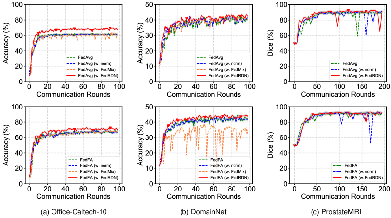
Figure 1: Illustration of test performance versus communication rounds on (a) Office-Caltech-10 [4], (b) DomainNet [24], and (c) ProstateMRI [20].

4.2 Main Results

In this section, we present the overall results on three benchmarks: Office-Caltech-10 and DomainNet in Table 1 and ProstateMRI in Table 2, including two different tasks, i.e., image classification, and medical image segmentation. For a detailed comparison, we present the test accuracy of each client and the average result.

All FL methods yield significant improvements combined with FedRDN consistently over three datasets. As we can see, FedRDN leads to consistent performance improvement for all FL baselines across three benchmarks compared with using the base data augmentation flow. The improvements of FedRDN can be large as 11.21% on Office-Caltech-10, 3.26% on DomainNet, and 1.37% on ProstateMRI, respectively. Especially for FedFA, the state-of-the-art FL method for feature distribution skewed FL setting, can still gain improvements, e.g., 3.27% on Office-Caltech-10. This indicates that input-level augmentation and feature-level augmentation are not contradictory and can be used simultaneously. Moreover, some weaker FL methods can even achieve better performance than others when using FedRDN. For example, after using FedRDN, the accuracy of FedAvg can be significantly higher than all other FL methods except FedFA, and FedProto can be even higher than FedFA. The above results demonstrate the effectiveness of the data-level solution, which can effectively mitigate the feature shift. Besides, compared with other robust FL methods, our method has a stronger scalability and generalization ability.

FedRDN is superior to other input-level data augmentation techniques. As shown in Table 1 and  2, FedRDN shows leading performance compared with conventional data normalization and FedMix, a previous input-level data augmentation technique. Besides, these two augmentation techniques can even decrease the performance of the method in several cases, while FedRDN can achieve consistent improvements. For instance, FedAvg and FedProto yield a drop as large as 1.05% and 3.54% with conventional data normalization on Office-Caltech-10, respectively. FedProx and FedFA show a drop as 0.67% and 5.54% on DomainNet, respectively, when they combined with FedMix. The above results demonstrated the effectiveness of FedRDN, and it has stronger generalizability compared with other data augmentation methods.

4.3 Communication Efficiency

Convergence  To explore the impact of various data augmentation techniques on the convergence, we draw the test performance curve of FedAvg and a state-of-the-art FL method, i.e., FedFA, with different communication rounds on three datasets as shown in Fig. 1. Apparently, FedRDN will not introduce any negative impact on the convergence of the method and even yield a faster convergence at the early training stage (0 $\sim$ 10 rounds) in some cases. As the training goes on, FedRDN achieves a more optimal solution. Besides, compared with other methods, the convergence curves of FedRDN are more stable.

Communication Cost  In addition to the existing communication overhead of FL methods, the additional communication cost in FedRDN is only for statistical information. The dimension of the statistic is so small (mean and standard deviation are $\mathbb{R}^{3}$ for RGB images), that the increased communication cost can be neglected. This is much different from the FedMix, which needs to share the average images per batch. The increased communication cost of FedMix is as large as 156MB on Office-Caltech-10 and 567MB on DomainNet while the batch size of averaged images is 5, even larger than the size of model parameters.

Table 3: Generalization performance of local model on Office-Caltech-10 [4]. We mark the best result in bold.

Source-site	Target-site	FedAvg	FedAvg + norm	FedAvg + FedMix [31]	FedAvg + FedRDN(Ours)
Amazon	Caltech	$48.00$	$48.09$	$42.22$	48.88
	DSLR	$46.87$	$44.41$	$59.37$	81.25
	Webcam	$77.96$	$77.96$	84.74	$83.05$
Caltech	Amazon	$58.33$	$58.85$	$51.56$	63.02
	DSLR	$68.75$	$68.75$	$75.00$	84.37
	Webcam	$83.05$	$83.05$	91.52	$86.35$
DSLR	Amazon	$42.70$	$41.14$	$33.85$	60.93
	Caltech	$33.33$	$35.11$	$35.55$	35.56
	Webcam	$79.66$	$77.96$	$74.57$	84.74
Webcam	Amazon	$53.64$	$55.20$	$47.91$	65.10
	Caltech	$41.33$	$43.55$	$40.00$	48.00
	DSLR	$68.75$	$68.75$	$78.12$	87.50

Table 4: The performance of FedRDN over FedRDN-V on three datasets.

Method	Office-Caltech-10	DomainNet	ProstateMRI [20]
FedAvg [23]	$62.51$	$42.32$	$90.02$
FedAvg [23] + FedRDN-V	$61.46$	$42.99$	$91.14$
FedAvg [23] + FedRDN (ours)	69.80	43.55	92.32

4.4 Cross-site Generalization performance

As stated before, FedRDN augments the data with luxuriant distribution from all clients to learn the generalized model. Therefore, we further explore the generalization performance of local models by cross-site evaluation, and the results are presented in Table 3. As we can see, All local models of FedRDN yield a solid improvement compared with the FedAvg and our method shows better generalization performance compared to other methods. The above results demonstrate that FedRDN can effectively mitigate the domain shift between different local datasets, which is beneficial to model aggregation. This is the reason why our method works.

4.5 Diagnostic Experiment

FedRDN vs. FedRDN-V  To deeply explore FedRDN, we develop a variant, FedRDN-V. Instead of randomly transforming, it transforms the images with the average mean $\hat{u}$ and standard deviation $\hat{\sigma}$ of all clients during training and testing phases:

$$\hat{u}=\sum_{k=1}^{K}\mu_{k},\quad\hat{\sigma}=\sum_{k=1}^{K}\sigma_{k}.$$ (8)

The results of comparison over three datasets are presented in Table 4. Apparently, FedRDN-V yields a significant drop compared with our method. This indicates the effectiveness of our method is not from the traditional data normalization but augmenting samples with the information from the multiple real local distributions. By this, each local model will be more generalized instead of biasing in skewed underlying distribution.

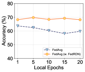
Figure 2: Illustration of test performance versus local epochs on Office-Caltech-10 [4].

Robust to Local Epochs  To explore the robustness of FedRDN for different local epochs, we tune the local epochs from the {1, 5, 10, 15, 20} and evaluate the performance of the learned model. The results are presented in Fig 2. Generally, more epochs of local training will increase the discrepancy under data heterogeneity, leading to slower convergence, which degrades the performance at the same communication rounds. The result of FedAvg validates this. By contrast, our method can obtain consistent improvements with different settings of local epochs. Moreover, our approach has stable performance across different local epoch settings due to effectively addressing the data heterogeneity.

Feature Distribution  To yield more insights about FedRDN, we utilize T-SNE [22] , a popular tool, to visualize the features of the global model before and after augmentation. Specifically, we visualize the features of test samples for each client and the results are shown in Fig 3. Apparently, FedRDN can help learn a more consistent feature distribution for different clients, while the learned feature of FedAvg is obviously biased, e.g., client 2 (DSLR). This validates what we previously stated: FedRDN is beneficial to learn more generalized features.

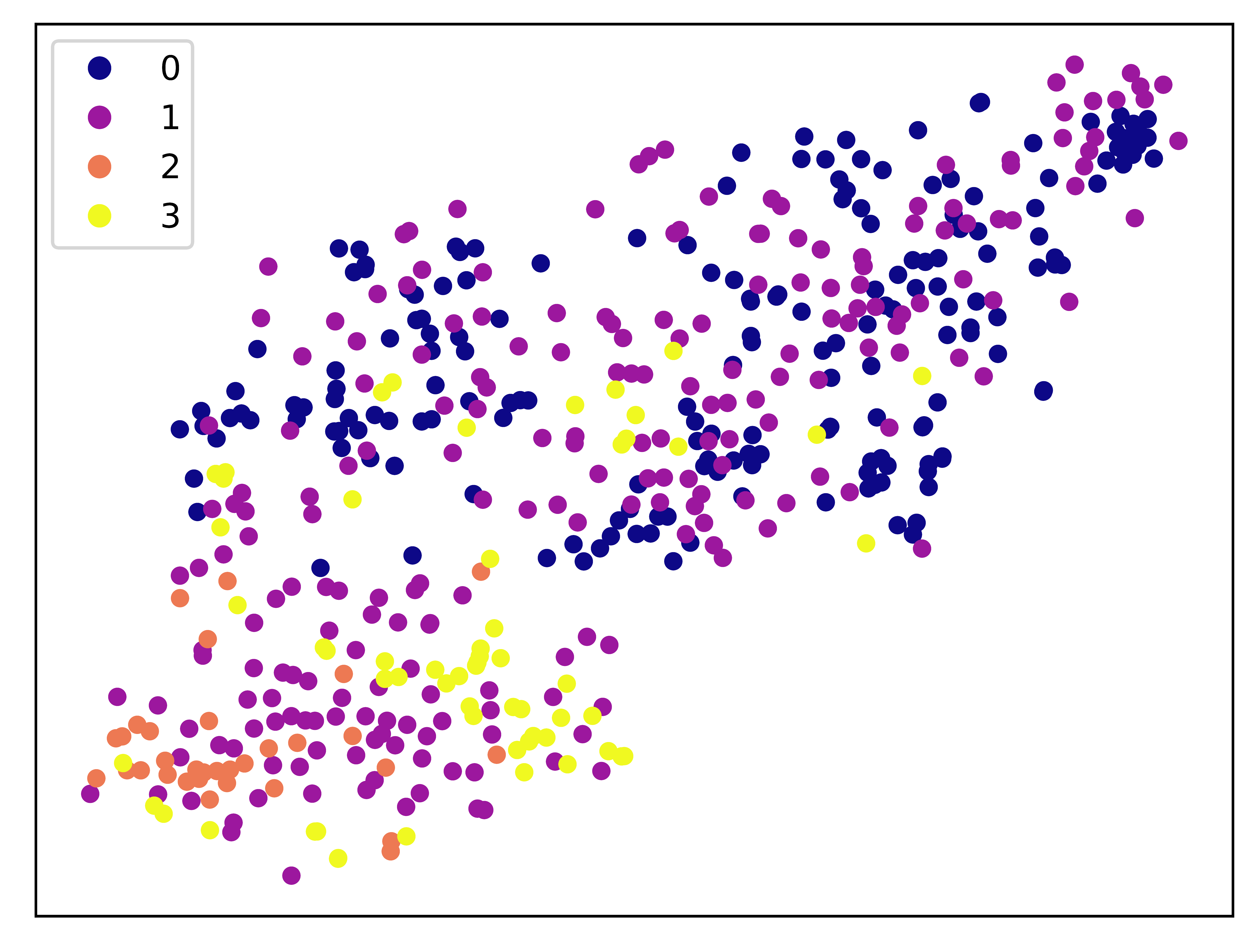
(a) FedAvg (colored by clients)

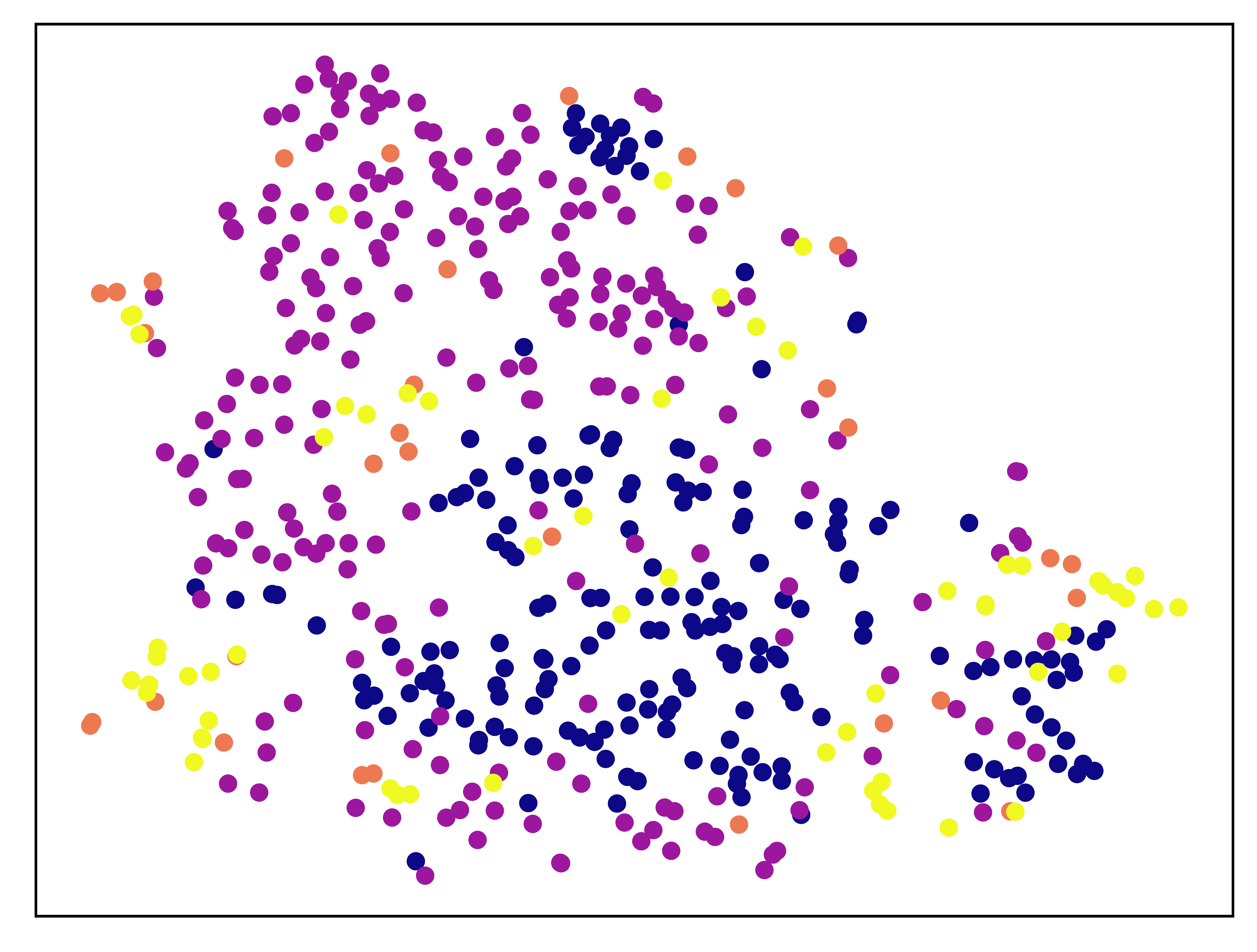
(b) FedAvg + FedRDN (colored by clients)

Figure 3: T-SNE visualization of features on Office-Caltech-10 [4]. The T-SNE is conducted on the test sample features of four clients.

5 Conclusion

In this paper, we focus on addressing the feature distribution skewed FL scenario. Different from the previous insights for this problem, we try to solve this challenge from the input-data level. The proposed novel data augmentation technique, FedRDN, is a plug-and-play component that can be easily integrated into the data augmentation flow, thereby effectively mitigating the feature shift. Our extensive experiments show that FedRDN can further improve the performance of various state-of-the-art FL methods across three datasets, which demonstrates the scalability, generalizability, and effectiveness of our method.

References

- [1] Acar, D.A.E., Zhao, Y., Matas, R., Mattina, M., Whatmough, P., Saligrama, V.: Federated learning based on dynamic regularization. In: International Conference on Learning Representations
- [2] Dong, J., Wang, L., Fang, Z., Sun, G., Xu, S., Wang, X., Zhu, Q.: Federated class-incremental learning. In: Proceedings of the IEEE/CVF Conference on Computer Vision and Pattern Recognition. pp. 10164–10173 (2022)
- [3] Fang, X., Ye, M.: Robust federated learning with noisy and heterogeneous clients. In: Proceedings of the IEEE/CVF Conference on Computer Vision and Pattern Recognition. pp. 10072–10081 (2022)
- [4] Gong, B., Shi, Y., Sha, F., Grauman, K.: Geodesic flow kernel for unsupervised domain adaptation. In: 2012 IEEE conference on computer vision and pattern recognition. pp. 2066–2073. IEEE (2012)
- [5] Hsu, T.M.H., Qi, H., Brown, M.: Measuring the effects of non-identical data distribution for federated visual classification. arXiv preprint arXiv:1909.06335 (2019)
- [6] Jiang, M., Wang, Z., Dou, Q.: Harmofl: Harmonizing local and global drifts in federated learning on heterogeneous medical images. In: Proceedings of the AAAI Conference on Artificial Intelligence. vol. 36, pp. 1087–1095 (2022)
- [7] Karimireddy, S.P., Kale, S., Mohri, M., Reddi, S., Stich, S., Suresh, A.T.: Scaffold: Stochastic controlled averaging for federated learning. In: International Conference on Machine Learning. pp. 5132–5143. PMLR (2020)
- [8] Krizhevsky, A., Sutskever, I., Hinton, G.E.: Imagenet classification with deep convolutional neural networks. Communications of the ACM 60(6), 84–90 (2017)
- [9] Kukačka, J., Golkov, V., Cremers, D.: Regularization for deep learning: A taxonomy. arXiv preprint arXiv:1710.10686 (2017)
- [10] Kumar, T., Turab, M., Raj, K., Mileo, A., Brennan, R., Bendechache, M.: Advanced data augmentation approaches: A comprehensive survey and future directions. arXiv preprint arXiv:2301.02830 (2023)
- [11] Lee, G., Jeong, M., Shin, Y., Bae, S., Yun, S.Y.: Preservation of the global knowledge by not-true distillation in federated learning. Advances in Neural Information Processing Systems (2021)
- [12] Li, B., Wu, F., Lim, S.N., Belongie, S., Weinberger, K.Q.: On feature normalization and data augmentation. In: Proceedings of the IEEE/CVF Conference on Computer Vision and Pattern Recognition. pp. 12383–12392 (2021)
- [13] Li, P., Li, D., Li, W., Gong, S., Fu, Y., Hospedales, T.M.: A simple feature augmentation for domain generalization. In: Proceedings of the IEEE/CVF International Conference on Computer Vision. pp. 8886–8895 (2021)
- [14] Li, Q., Diao, Y., Chen, Q., He, B.: Federated learning on non-iid data silos: An experimental study. In: 2022 IEEE 38th International Conference on Data Engineering (ICDE). pp. 965–978. IEEE (2022)
- [15] Li, Q., He, B., Song, D.: Model-contrastive federated learning. In: Proceedings of the IEEE/CVF International Conference on Computer Vision. pp. 10713–10722 (2021)
- [16] Li, T., Sahu, A.K., Talwalkar, A., Smith, V.: Federated learning: Challenges, methods, and future directions. IEEE signal processing magazine 37(3), 50–60 (2020)
- [17] Li, T., Sahu, A.K., Zaheer, M., Sanjabi, M., Talwalkar, A., Smith, V.: Federated optimization in heterogeneous networks. Proceedings of Machine Learning and Systems 2, 429–450 (2020)
- [18] Li, X., Jiang, M., Zhang, X., Kamp, M., Dou, Q.: Fedbn: Federated learning on non-iid features via local batch normalization. arXiv preprint arXiv:2102.07623 (2021)
- [19] Lin, T., Kong, L., Stich, S.U., Jaggi, M.: Ensemble distillation for robust model fusion in federated learning. Advances in Neural Information Processing Systems 33, 2351–2363 (2020)
- [20] Liu, Q., Dou, Q., Yu, L., Heng, P.A.: Ms-net: multi-site network for improving prostate segmentation with heterogeneous mri data. IEEE transactions on medical imaging 39(9), 2713–2724 (2020)
- [21] Luo, M., Chen, F., Hu, D., Zhang, Y., Liang, J., Feng, J.: No fear of heterogeneity: Classifier calibration for federated learning with non-iid data. Advances in Neural Information Processing Systems 34, 5972–5984 (2021)
- [22] Van der Maaten, L., Hinton, G.: Visualizing data using t-SNE. Journal of Machine Learning Research 9(11) (2008)
- [23] McMahan, B., Moore, E., Ramage, D., Hampson, S., y Arcas, B.A.: Communication-efficient learning of deep networks from decentralized data. In: Artificial intelligence and statistics. pp. 1273–1282. PMLR (2017)
- [24] Peng, X., Bai, Q., Xia, X., Huang, Z., Saenko, K., Wang, B.: Moment matching for multi-source domain adaptation. In: Proceedings of the IEEE/CVF international conference on computer vision. pp. 1406–1415 (2019)
- [25] Peng, X., Huang, Z., Zhu, Y., Saenko, K.: Federated adversarial domain adaptation. In: International Conference on Learning Representations
- [26] Reisizadeh, A., Farnia, F., Pedarsani, R., Jadbabaie, A.: Robust federated learning: The case of affine distribution shifts. Advances in Neural Information Processing Systems 33, 21554–21565 (2020)
- [27] Ronneberger, O., Fischer, P., Brox, T.: U-net: Convolutional networks for biomedical image segmentation. In: Medical Image Computing and Computer-Assisted Intervention–MICCAI 2015: 18th International Conference, Munich, Germany, October 5-9, 2015, Proceedings, Part III 18. pp. 234–241. Springer (2015)
- [28] Tan, Y., Long, G., Liu, L., Zhou, T., Lu, Q., Jiang, J., Zhang, C.: Fedproto: Federated prototype learning across heterogeneous clients. In: Proceedings of the AAAI Conference on Artificial Intelligence. vol. 36, pp. 8432–8440 (2022)
- [29] Venkataramanan, S., Kijak, E., Amsaleg, L., Avrithis, Y.: Alignmixup: Improving representations by interpolating aligned features. In: Proceedings of the IEEE/CVF Conference on Computer Vision and Pattern Recognition (CVPR). pp. 19174–19183 (June 2022)
- [30] Wang, J., Liu, Q., Liang, H., Joshi, G., Poor, H.V.: Tackling the objective inconsistency problem in heterogeneous federated optimization. Advances in Neural Information Processing Systems 33 (2020)
- [31] Yoon, T., Shin, S., Hwang, S.J., Yang, E.: Fedmix: Approximation of mixup under mean augmented federated learning. arXiv preprint arXiv:2107.00233 (2021)
- [32] Yun, S., Han, D., Oh, S.J., Chun, S., Choe, J., Yoo, Y.: Cutmix: Regularization strategy to train strong classifiers with localizable features. In: Proceedings of the IEEE/CVF international conference on computer vision. pp. 6023–6032 (2019)
- [33] Yurochkin, M., Agarwal, M., Ghosh, S., Greenewald, K., Hoang, N., Khazaeni, Y.: Bayesian nonparametric federated learning of neural networks. In: International conference on machine learning. pp. 7252–7261. PMLR (2019)
- [34] Zhang, H., Cisse, M., Dauphin, Y.N., Lopez-Paz, D.: mixup: Beyond empirical risk minimization. In: International Conference on Learning Representations
- [35] Zhang, J., Li, Z., Li, B., Xu, J., Wu, S., Ding, S., Wu, C.: Federated learning with label distribution skew via logits calibration. In: International Conference on Machine Learning. pp. 26311–26329. PMLR (2022)
- [36] Zhong, Z., Zheng, L., Kang, G., Li, S., Yang, Y.: Random erasing data augmentation. In: Proceedings of the AAAI conference on artificial intelligence. vol. 34, pp. 13001–13008 (2020)
- [37] Zhou, T., Konukoglu, E.: Fedfa: Federated feature augmentation. International Conference on Learning Representations (2023)