Causal Classification of Spatiotemporal Quantum Correlations

Abstract

From correlations in measurement outcomes alone, can two otherwise isolated parties establish whether such correlations are atemporal? That is, can they rule out that they have been given the same system at two different times? Classical statistics says no, yet quantum theory disagrees. Here, we introduce the necessary and sufficient conditions by which such quantum correlations can be identified as atemporal. We demonstrate the asymmetry of atemporality under time reversal, and reveal it to be a measure of spatial quantum correlation distinct from entanglement. Our results indicate that certain quantum correlations possess an intrinsic arrow of time, and enable classification of general quantum correlations across space-time based on their (in)compatibility with various underlying causal structures.

I Introduction

Consider Alice and Bob, situated in their own laboratories. In each round, they each receive correlated random variables $A$ and $B$. The correlations were distributed via one of three possible causal mechanisms: (i) spatially such that $A$ and $B$ share a common cause, (ii) temporally such that measurement outcomes of $A$ are communicated to $B$ or vice versa, and (iii) some combination of the above (see Fig. 1). Alice and Bob record these correlations. With only this recording, can we rule out one of the causal mechanisms above? Classical statistics says no. The observed correlations will always be compatible with all possible scenarios. Thus the idiom ‘correlation does not imply causation’.

Quantum correlations can exhibit remarkable differences from classical ones. Suppose Alice and Bob each receive a single qubit each round, which they then measure in some Pauli basis. The correlations between their measurement outcomes can lie outside what a density operator describes. Such aspatial correlations cannot be explained purely by a common cause (see Fig. 1a), leading to quantum correlations that can indeed imply causation [1, 2]. There is thus significant interest in quantum causal inference  [1, 3, 4, 5, 2, 6], due to its stark departure from classical statistics.

Here we ask, do certain quantum correlations require a common cause? We answer in the affirmative by formalizing the notion of atemporal quantum correlations – correlations between Alice and Bob’s qubit measurements that cannot be explained by purely temporal means (i.e., as two measurements on a qubit communicated by some quantum channel between Alice and Bob, see Fig. 1b). We demonstrate computable necessary and sufficient indicators for atemporality and demonstrate that (1) it is asymmetric under time-reversal and thus reveals the existence of correlations possessing an intrinsic arrow of time, and (2) it represents a new operational form of non-classical correlations distinct from entanglement. This induces a framework for causal classification – classifying general spatiotemporal quantum correlations based on their compatibility with various causal distribution mechanisms. Our results thus provide new mathematical tools and concepts for understanding how quantum correlations can infer causal structure in ways without classical analogs.

II Results

Framework. Returning to the opening scenario where Alice and Bob are in their own laboratories, we label the qubits Alice and Bob each possess respectively by $A$ and $B$. We assume that the qubit pair is prepared in the same way in each round. Such a preparation scheme may be:

• Spatially distributed, such that $A$ and $B$ correspond to two parts of some bipartite state $\bm{\rho}_{AB}$ (see Fig. 1a).

• Temporally distributed, such that $B$ is the output of $A$ subject to some fixed quantum channel (completely-positive trace-preserving map) $\mathcal{E}$, or vice versa (see Fig. 1b).

• Neither purely spatially nor temporally distributed, such as when $A$ evolves to $B$ via non-Markovian evolution [7], or, more generally, when $A$ and $B$ are related by general process matrices [8] (see Fig. 1c).

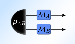
(a) Spatially distributed

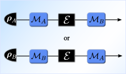
(b) Temporally distributed

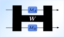
(c) General spatiotemporally distributed

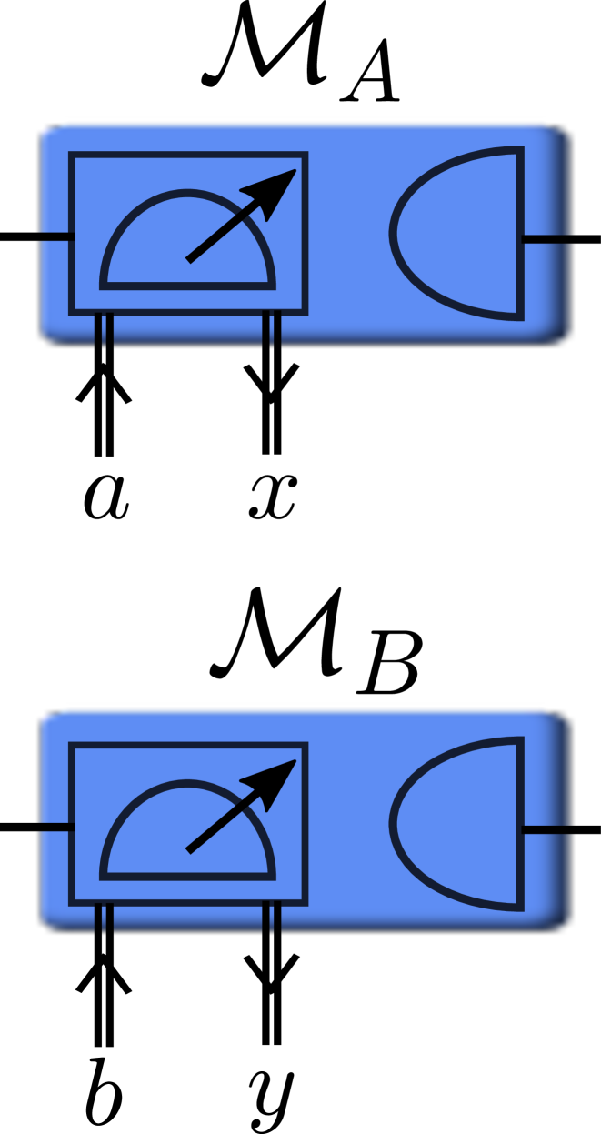
Figure 1: Correlations distribution mechanisms. Consider Alice and Bob that makes respective projective measurements $\mathcal{M}_{A}$ and $\mathcal{M}_{B}$ on respective quantum systems $A$ and $B$ (blue boxes). We divide potential mechanisms of correlating these measurements into three categories: (a) purely spatially-distributed mechanisms involving $A$ and $B$ being two aims of some bipartite state $\rho_{AB}$, reflecting the case of common cause, (b) purely temporally-distributed such that $A$ and $B$ represent the input and output of some quantum channel $\mathcal{E}$, reflecting the case of direct cause, or (c) some combination of both, representing general non-Markovian evolution or cases of indefinite causal order [8]. We refer to correlations that are incompatible with (a) as aspatial and those incompatible with (b) as atemporal.

Let $\bm{\sigma}_{0}=\mathbf{I}$, $\bm{\sigma}_{1}=\mathbf{X}$, $\bm{\sigma}_{2}=\mathbf{Y}$, $\bm{\sigma}_{3}=\mathbf{Z}$ be the identity and the three standard Pauli operators . Let $\Pr(x,y|a,b)$ then denote the probability of Alice getting outcome $x$ and Bob getting outcome $y$ when Alice chooses to measure in basis $\bm{\sigma}_{a}$ and Bob in $\bm{\sigma}_{b}$. Alice and Bob do not perform any other interventions. By choosing appropriate Pauli measurements over a large number of rounds, Alice and Bob can determine the expectation values $\expectationvalue{\bm{\sigma}_{a},\bm{\sigma}_{b}}=\sum_{x,y}xy\Pr(x,y|a,b)$ describing how their measurement outcomes correlate in various Pauli basis to any desired level of accuracy. Alice and Bob then pass this information to us. Using this information, what can we conclude about the causal mechanism behind the preparation of $A$ and $B$?

Given Pauli correlations $\expectationvalue{\bm{\sigma}_{a},\bm{\sigma}_{b}}$ for each $a,b\in\{0,1,2,3\}$, we can describe the information received concisely via the pseudo-density operator (PDO)

$$\mathbf{R}_{AB}\equiv\sum_{a,b=0}^{3}\frac{\expectationvalue{\bm{\sigma}_{a},\bm{\sigma}_{b}}}{4}\bm{\sigma}_{a}\otimes\bm{\sigma}_{b}.$$

Such PDOs were initially proposed to identify quantum correlations that imply causality [2] and have seen various uses towards building quantum information theories that place space and time on equal footing [6, 10, 11]. They contain all the information about $\expectationvalue{\bm{\sigma}_{a},\bm{\sigma}_{b}}$, since the latter can be retrieved directly via $\expectationvalue{\bm{\sigma}_{a},\bm{\sigma}_{b}}=\tr[\mathbf{R}_{AB}(\bm{\sigma}_{a}\otimes\bm{\sigma}_{b})]$. Thus our capacity to infer causal mechanisms from the Pauli correlations coincides with our capacity to infer causal mechanisms from the corresponding PDO. Also note that when qubits $A$ and $B$ are spatially distributed, $\mathbf{R}_{AB}$ reduces to a standard density operator. Meanwhile, their marginal distributions are always positive and describe local measurement statistics for Alice and Bob.
Spatial and temporal compatibility. We introduce two distinct criteria on PDOs: We say that $\mathbf{R}_{AB}$ is spatially compatible, or belongs to $\mathcal{S}$ if its statistics can be generated via a spatial distribution mechanism (i.e., as in Fig. 1a). Similarly, we say that $\mathbf{R}_{AB}$ is temporally compatible, or belongs to $\mathcal{T}$ if its statistics can be generated via a temporal distribution mechanism (i.e., as in Fig. 1b). We will often use the terms spatial and temporal for brevity, but we stress that they only mean compatible with a spatially or temporally distributed structure. PDOs that lie outside of $\mathcal{S}$ are referred to as aspatial, and those that lie outside of $\mathcal{T}$ are referred to as atemporal.

We then divide the set of all PDOs using a Venn diagram into four separate classes based on their spatial-temporal compatibility: Those that (a) lie in $\mathcal{S}$ and $\mathcal{T}$ and are thus compatible with any distribution mechanism, (b) lie in $\mathcal{S}$ but not $\mathcal{T}$ and thus rule out purely temporal distribution mechanisms, (c) lie in $\mathcal{T}$ but not $\mathcal{S}$ and thus rule out purely spatial distribution mechanisms and (d) those that lie outside $\mathcal{S}$ and $\mathcal{T}$ that cannot be explained by either purely spatial or temporal distribution scheme but rather, rely on a more complicated combination of spatial and temporal mechanisms. All classical states (those with positive, diagonal PDOs) lie within (a). We cannot infer anything conclusive about the causal mechanism in alignment with classical statistics. Quantum correlations, however, permit PDOs in each of (b), (c), and (d), where certain causal mechanisms can be ruled out (see Fig. 2).

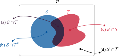
Figure 2: Venn diagram of all spatial–temporal compatibility. The set $\mathcal{P}$ of observed spatiotemporal quantum correlations (as described by PDOs) is divided into four mutually exclusive subsets: (a) $\mathcal{S}\cap\mathcal{T}$ represent correlations that are compatible with pure spatially and pure temporal causal mechanisms. Examples include all classical correlations and separable Werner states [12], (b) $\mathcal{S}\cap\mathcal{T}^{c}$ represents correlations that rule out purely temporal distribution mechanisms. Examples include Bell and entangled Werner states, (c) $\mathcal{S}^{c}\cap\mathcal{T}$ represents correlations that rule out purely spatial causal mechanisms such as two coexisting qubits measured separately, and (d) $\mathcal{S}^{c}\cap\mathcal{T}^{c}$ designates correlations that require a combination of causal distribution mechanisms to explain. An example is the application of two different temporal PDOs conditioned on some external degree of freedom. Note that unlike $\mathcal{S}$, $\mathcal{T}$ does not form a convex set (see 5 in Methods).

To better understand what PDOs lie within each class, we need a necessary and sufficient criterion for aspatiality and atemporality. Past studies of causality have focused on the former, showing that the negativity of $\mathbf{R}_{AB}$ is necessary and sufficient for aspatiality. We will derive analogous conditions for when a PDO is atemporal, and thus build a full picture of spatial-temporal compatibility.

Certifying atemporality. Given $\mathbf{R}_{AB}$, our goal is to determine identifiers of atemporality that rule out compatibility with temporal distribution mechanisms. Consider first a forward atemporality measure $\overrightarrow{f}$ that is zero if and only if $\mathbf{R}_{AB}$ has statistics consistent with a temporal distribution mechanism from $A$ to $B$; and a reverse atemporality measure $\overleftarrow{f}$ that is zero if and only if $\mathbf{R}_{AB}$ has statistics consistent with a temporal distribution mechanism from $B$ to $A$. Together they naturally induce a general atemporality measure $f=\mathrm{min}(\overrightarrow{f},\overleftarrow{f})$ that is zero if and only if $\mathbf{R}_{AB}$ lies in $\mathcal{T}$.

We then introduce pseudo-channels, a temporal analogue of pseudo-density operators. Recall that the Choi–Jamiołkowski isomorphism [13] allows us to represent each qubit channel $\Lambda$ by a Choi operator

$$\bm{{\mathchoice{\raisebox{0.0pt}{$\displaystyle\chi$}}{\raisebox{0.0pt}{$\textstyle\chi$}}{\raisebox{0.0pt}{$\scriptstyle\chi$}}{\raisebox{0.0pt}{$\scriptscriptstyle\chi$}}}}_{\Lambda}\equiv(\mathcal{I}\otimes\Lambda)\ket{\phi^{+}}\!\bra{\phi^{+}},$$

describing the output state when $\Lambda$ is applied to one arm of a Bell state $\ket{\phi^{+}}=\frac{1}{\sqrt{2}}(\ket{00}+\ket{11})$, where $\mathcal{I}$ denotes the identity channel. This output, however, does not need to be a valid spatial quantum state if $\Lambda$ is not a valid quantum channel. More generally, let $\bm{{\mathchoice{\raisebox{0.0pt}{$\displaystyle\chi$}}{\raisebox{0.0pt}{$\textstyle\chi$}}{\raisebox{0.0pt}{$\scriptstyle\chi$}}{\raisebox{0.0pt}{$\scriptscriptstyle\chi$}}}}_{\Lambda}$ be a PDO with non-zero negativity $\mathcal{N}(\bm{{\mathchoice{\raisebox{0.0pt}{$\displaystyle\chi$}}{\raisebox{0.0pt}{$\textstyle\chi$}}{\raisebox{0.0pt}{$\scriptstyle\chi$}}{\raisebox{0.0pt}{$\scriptscriptstyle\chi$}}}}_{\Lambda})$ (absolute sum of its negative eigenvalues). In such scenarios, $\Lambda$ remains trace-preserving and linear, but is no longer completely positive. We say that $\Lambda$ is a pseudo-channel, and $\mathcal{N}(\bm{{\mathchoice{\raisebox{0.0pt}{$\displaystyle\chi$}}{\raisebox{0.0pt}{$\textstyle\chi$}}{\raisebox{0.0pt}{$\scriptstyle\chi$}}{\raisebox{0.0pt}{$\scriptscriptstyle\chi$}}}}_{\Lambda})$ provides a necessary and sufficient indicator of its non-physicality.

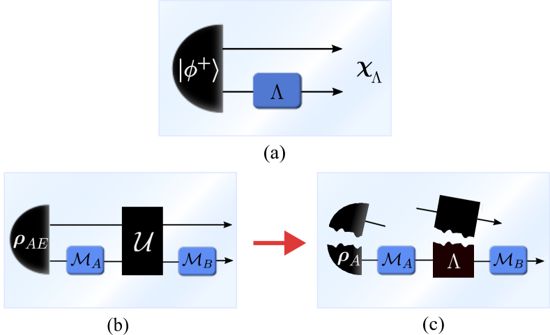
Figure 3: Choi operator and pseudo-channels. (a) The Choi operator of a quantum channel $\Lambda$ describes the resulting state when we apply $\Lambda$ on one arm of the Bell state $\ket{\phi^{+}}\equiv\frac{1}{\sqrt{2}}(\ket{00}+\ket{11})$. (b) In cases where the resulting correlations $\mathbf{R}_{AB}$ between $A$ and $B$ are atemporal such as that of non-Markovian evolution, there is no valid quantum channel from $A$ to $B$. (c) Nevertheless, we can identify a pseudo-channel $\Lambda$ that forcibly interprets the dynamics as though it is a Markovian map. The resulting $\Lambda$ is non-physical, which is reflected by the negativity of its Choi operator. We show that this negativity is a necessary and sufficient condition for the forward atemporality of $\mathbf{R}_{AB}$.

Such pseudo-channels provide a natural means to define $\overrightarrow{f}$ (and thus $\overleftarrow{f}$ and $f$). Given $\mathbf{R}_{AB}$, we first assert that it describes correlations resulting from some quantum channel $\overrightarrow{\Lambda}$ with input system $A$ and output system $B$. Such a $\overrightarrow{\Lambda}$ would then satisfy

$$\mathbf{R}_{AB}=\left(\mathcal{I}_{A}\otimes\overrightarrow{\Lambda}\right)\mathbf{K}_{AB}$$ (1)

where $\mathbf{K}_{AB}\equiv\left\{\bm{\rho}_{A}\otimes\frac{\mathbf{I}_{B}}{2},\mathbf{S}_{AB}\right\}$ with $\bm{\rho}_{A}\equiv\tr_{B}\mathbf{R}_{AB}$ being the first marginal, $\{\cdot,\cdot\}$ the anti-commutator, $\mathbf{I}$ the identity operator, and $\mathbf{S}$ the swap operator [6, 14]. When $\mathbf{R}_{AB}$ is incompatible with a temporal distribution mechanism from $A$ to $B$, no such valid quantum channels exist. However, we can drop the complete-positivity requirements on $\overrightarrow{\Lambda}$. This allows us to interpret any spatiotemporal correlations as resulting from a pseudo-channel $\overrightarrow{\Lambda}$ acting on $A$ to generate $B$ (see Fig. 3). The minimal non-physicality of such a channel then motivates our definition for forward atemporality:

$$\overrightarrow{f}(\mathbf{R}_{AB})\equiv\min_{\overrightarrow{\Lambda}}~{}\mathcal{N}(\bm{{\mathchoice{\raisebox{0.0pt}{$\displaystyle\chi$}}{\raisebox{0.0pt}{$\textstyle\chi$}}{\raisebox{0.0pt}{$\scriptstyle\chi$}}{\raisebox{0.0pt}{$\scriptscriptstyle\chi$}}}}_{\overrightarrow{\Lambda}}),$$ (2)

where the minimization is over all forward pseudo-channels $\overrightarrow{\Lambda}$ that is compatible with $\mathbf{R}_{AB}$. Similarly, we define the reverse atemporality $\overleftarrow{f}$ by interchanging the roles of $A$ and $B$, thus also defining the general atemporality $f=\mathrm{min}(\overrightarrow{f},\overleftarrow{f})$. For example, the entangled Bell state $\frac{1}{\sqrt{2}}(\ket{01}-\ket{10})$ has forward, reverse and total atemporality of $0.5$ (its corresponding pseudo-channel being the non-physical universal-NOT gate [15]). This then leads to one of our key results:

Result 1.

Given spatiotemporal correlations described by a PDO $\mathbf{R}_{AB}$, let

$$\overrightarrow{f}(\mathbf{R}_{AB})\equiv\min_{\overrightarrow{\Lambda}}~{}\mathcal{N}(\bm{{\mathchoice{\raisebox{0.0pt}{$\displaystyle\chi$}}{\raisebox{0.0pt}{$\textstyle\chi$}}{\raisebox{0.0pt}{$\scriptstyle\chi$}}{\raisebox{0.0pt}{$\scriptscriptstyle\chi$}}}}_{\overrightarrow{\Lambda}}),$$ (3)

where the minimization is over all forward pseudo-channels $\overrightarrow{\Lambda}$ that is compatible with $\mathbf{R}_{AB}$ (i.e., those that satisfy Eq. (1)). Then $f>0$ is a necessary and sufficient condition for atemporality. Moreover, we have a systematic algorithm (see below) to compute $\overrightarrow{f}$ for any $\mathbf{R}_{AB}$.

To establish the above, first observe that $f>0$ implies that no physical channel is compatible with $\mathbf{R}_{AB}$ by definition. Meanwhile, $\mathbf{R}_{AB}$ being atemporal necessitating $f>0$ requires each $\mathbf{R}_{AB}$ to have at least one compatible forward pseudo-channel (see 1 in Methods). We establish this by introducing a systematic method to identify such compatible pseudo-channels $\overrightarrow{\Lambda}$ (as expressed by their Choi operator). When $\mathbf{R}_{AB}$ has full rank marginals, $\overrightarrow{\Lambda}$ is unique and the algorithm that returns its Choi operator $\textstyle\chi$ is particularly simple (see Algorithm 1). From this, the forward atemporality can be directly computed.

Algorithm 1 Choi operator of pseudo-channel construction

1:$2$-qubit PDO $\mathbf{R}_{AB}$

2:$\bm{\rho}_{A}\leftarrow\tr_{B}\mathbf{R}_{AB}$

3:$\mathbf{L}\leftarrow\left(\bm{\rho}_{A}-\frac{\mathbf{I}}{2}\right)\otimes\tr_{A}\left[\left(\frac{1}{2}\bm{\rho}_{A}^{-1}\otimes\mathbf{I}\right)\mathbf{R}_{AB}\right]+\frac{\mathbf{I}}{2}\otimes\tr_{A}\left[\left((\mathbf{I}-\frac{1}{2}\bm{\rho}_{A}^{-1})\otimes\mathbf{I}\right)\mathbf{R}_{AB}\right]$

4:$\bm{{\mathchoice{\raisebox{0.0pt}{$\displaystyle\chi$}}{\raisebox{0.0pt}{$\textstyle\chi$}}{\raisebox{0.0pt}{$\scriptstyle\chi$}}{\raisebox{0.0pt}{$\scriptscriptstyle\chi$}}}}\leftarrow(T\otimes\mathcal{I})(\mathbf{R}_{AB}-\mathbf{L})$ $\triangleright$ $T$ denotes the transpose map

5:return $\textstyle\chi$

When the first marginal $\bm{\rho}_{A}$ is rank-deficient (i.e., some pure state $\outerproduct{\phi}{\phi}$), the pseudo-channels compatible with $\mathbf{R}_{AB}$ are no longer unique. This is because any such causal interpretation corresponds to Alice being given a system in $\ket{\phi}$, such that measured statistics do not contain the resulting state $\bm{\tau}$ when $\Lambda$ acts on state $\ket{\smash{\phi^{\perp}}}$ perpendicular to $\ket{\phi}$. In Methods, we generalize the above algorithm to identify all compatible pseudo-channels, and a semi-definite program to find the minimum non-physicality among them. Thus, we can systematically evaluate the forward atemporality $\overrightarrow{f}$ for all two-qubit PDOs. Interchanging roles of $A$ and $B$ enables evaluation of the reverse atemporality $\overleftarrow{f}$ and thus overall atemporality $f$.

Properties of atemporality. The computability of atemporality offers efficient means to study its properties. Here, we survey key results (see Supplementary Information A and B for further details). The first is time-reversal asymmetry. Unlike classical correlations, certain quantum correlations admit temporal causal mechanisms in only one temporal direction.

Result 2.

Forward atemporality does not imply reverse atemporality or vice versa.

Consider a PDO describing a single qubit undergoing probabilistic dephasing (see Fig. 4). Clearly, its forward atemporality is $0$ by construction. However, $\overleftarrow{f}(\mathbf{R}_{AB})>0$ for all $p\neq 0,1$. Thus, quantum correlations not only can imply causality as previously suggested [2, 1], but can also only imply causality in a particular temporal direction.

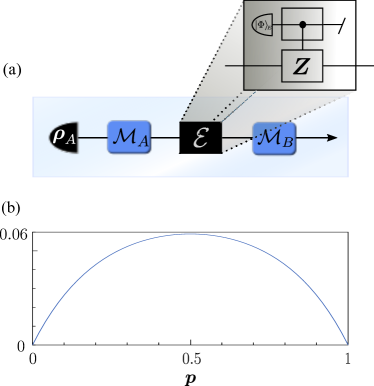
Figure 4: Time-reversal asymmetry of atemporality. (a) Consider a quantum circuit where a qubit $A$ initially in state $\bm{\rho}_{A}=\frac{1}{4}\ket{+}\!\bra{+}+\frac{3}{4}\ket{-}\!\bra{-}$ is subject to a quantum channel $\mathcal{E}(\bm{\rho}):=p\bm{\rho}+(1-p)\mathbf{Z}\bm{\rho}\mathbf{Z}^{\dagger}$, the output of which we label qubit $B$. One can implement this temporal process by a controlled-$Z$ gate with an ancillary system $E$, prepared in a state $\ket{\Phi}_{E}=\sqrt{p}\ket{0}+\sqrt{1-p}\ket{1}$. Clearly, the correlations between $A$ and $B$ admit a temporal distribution mechanism from $A$ to $B$. (b) However, its reverse atemporality is non-zero and thus has no causal interpretation from $B$ to $A$.

The interplay of temporal and spatial compatibility is also a natural point of interest. Specifically, let us restrict ourselves to density operators (i.e., correlations that lie in $\mathcal{S}$). In Supplementary Information A, we show that all classically correlated states (i.e., those with zero discord  [16, 17, 18]) have zero atemporality – in agreement with our understanding that classical statistics cannot rule out any causal mechanism without active intervention.

Given the above, one might speculate that entanglement implies atemporality. Indeed, in Methods we show whenever $\mathbf{R}\in\mathcal{S}$ is pure or its marginals are given by the maximally mixed state (see 3 in Methods), that non-zero atemporality coincides with non-zero entanglement. However, this does not hold in more general conditions:

Result 3.

Entanglement does not imply atemporality: Certain entangled states are temporally compatible.

Consider the parameterized family of biased Werner states $\bm{\rho}_{p,q}^{\text{B.W.}}\equiv(1-p)\bm{\rho}^{\text{Werner}}_{q}+p\ket{00}\!\bra{00}$, achieved by mixing a standard Werner state $\bm{\rho}^{\text{Werner}}_{q}$ with the state $\outerproduct{00}{00}$ (see Fig. 5). Here, $\bm{\rho}_{0.5,0.25}^{\text{B.W.}}$ has zero atemporality, but non-zero entanglement negativity ($\approx 0.0087$) [20]. Nevertheless, sufficiently strong entanglement does guarantee atemporality. In Methods (see Eq. 6 in Methods) we prove the following:

Result 4.

Any temporally compatible $2$-qubit state must have entanglement negativity of at most $\frac{1}{2}(\sqrt{2}-1)$.

Indeed a scatter plot of atemporality vs. entanglement negativity for 1000 randomly PDOs suggest that two concepts are heavily correlated but not the same – with atemporality looking to be a stronger notion of non-classical correlations than entanglement (see Supplementary Information A). Thus we anticipate that future study of atemporality could well lead to a new and finer-grained understanding of quantum correlations.

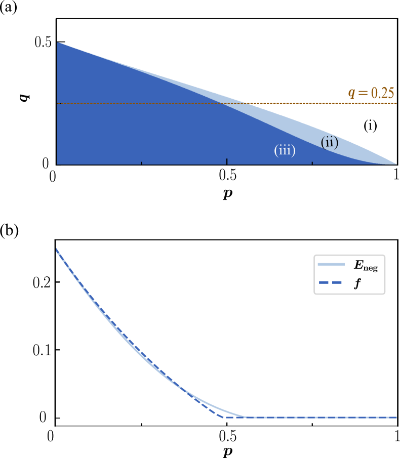
Figure 5: Entanglement and atemporality. The family of biased Werner states $\bm{\rho}_{p,q}^{\text{B.W.}}\equiv(1-p)\bm{\rho}^{\text{Werner}}_{q}+p\ket{00}\!\bra{00}$ illustrates the differences between entanglement and atemporality. (a) depicts a colour map depicting entanglement and atemporality of $\bm{\rho}_{p,q}^{B.W.}$ for various values of $p$ and $q$. While (i) all separable states are not atemporal, (ii) there exist entangled states that nevertheless admit temporal distribution mechanisms. Notwithstanding, (iii) most entangled states within the family are atemporal. (b) Indeed, at $q=0.25$, there is a region where the entanglement negativity $E_{\text{neg}}$ of $\bm{\rho}_{p,q}^{\text{B.W.}}$ is non-zero and atemporality $f$ is zero.

III Discussion

Spatiotemporal quantum correlations differ crucially from classical counterparts in that they can be fundamentally incompatible with certain underlying causal mechanisms. In this article, we showed that such correlations between various Pauli measurements on two qubits $A$ and $B$ can be atemporal, such that their explanation necessitates some common cause. We provided a necessary and sufficient indicator of atemporality and a systematic algorithm to compute it. In studying atemporality, we illustrated (1) the existence of temporal asymmetry – whereby certain correlations admit purely causal explanations in only one temporal direction and (2) that atemporality induces a notion of quantum correlations distinct from entanglement. Combined with prior work showing quantum correlations can also be aspatial – such that they cannot be purely explained by a common cause – our results enable a framework to classify quantum correlations based on their compatibility with spatial and temporal causal mechanisms.

This classification opens a number of interesting directions. Like spatial correlations, a complete understanding of atemporality will be a highly involved affair. Conceptually, atemporality between $A$ and $B$ measures how non-physical’ a quantum channel from $A$ and $B$ (or vice versa) must be to generate the correlations observed. Here we analyzed one particular mathematical definition of non-physicality (negativity of their corresponding Choi operator). This choice is not unique; other definitions of non-physical maps and quantifiers of non-physicality have been proposed in the context of understanding non-Markovianity [21, 22, 23, 24, 25, 26, 27] (Indeed, Atemporality can also be considered as a marker of non-Markovianity). More generally, PDOs simply describe one possible set of measurement statistics between two observers at different points in space-time. We can certainly consider other measurement statistics (e.g. quadrature correlations between optical modes with a recently proposed PDO analogue [28]), and thus anticipate a plethora of possible atemporality measures and indicators that mirror the diversity of current works studying spatial quantum correlations. S

Meanwhile, the relation between atemporality and spatial quantum correlations also yields fascinating insights. We proved that some forms of quantum correlation are required for a standard bipartite quantum system to be temporal and sufficient entanglement guarantees atemporality. Still, many open questions remain. Some entangled states are not atemporal, so is atemporality a strictly stronger notion of quantum correlations? And if so, is it guaranteed by steering or Bell non-locality [29]? We also have no proof that atemporality guarantees entanglement, and thus could atemporality persist in more robust forms of quantum correlations [18]? Whatever the case, atemporality has a clear operational interpretation and introduces an entirely new category to the existing hierarchy of quantum correlations, and answering such questions will help us better understand the uniquely quantum incompatibility between spatial and temporal correlations.

IV Methods

Temporal PDOs. Imagine that Alice and Bob have qubit systems, $A$ and $B$, respectively, and they had been temporally distributed where measurements on the system $A$ occur before measurements on the system $B$. Namely, the system $A$ is initially prepared in some state $\bm{\rho}_{A}$ and the system $B$ is the result of acting some fixed quantum channel $\mathcal{E}$ on the post-measurement state of the qubit $A$. Each round, Alice and Bob implement Pauli measurements in their choices $a,b$ of basis. In this scenario, the joint probability $\Pr(xy|ab)$ to obtain the measurement outcome $x,y$ is given by

$$\Pr(xy|ab)=\tr[\mathcal{E}\bigl{(}\bm{\Pi}_{x|a}\bm{\rho}_{A}\bm{\Pi}_{x|a}\bigr{)}\bm{\Pi}_{y|b}\Bigr{]},$$

where $\bm{\Pi}_{x|a},\bm{\Pi}_{y|b}$ denotes the projection operator to $x,y$ of the Pauli operator $\bm{\sigma}_{a},\bm{\sigma}_{b}$, respectively. From this we have expectation values $\expectationvalue{\bm{\sigma}_{a},\bm{\sigma}_{b}}$:

$$\begin{aligned} \expectationvalue{\bm{\sigma}_{a},\bm{\sigma}_{b}}&\equiv\sum_{xy}xy\cdot\Pr(xy|ab)\\ &=\sum_{xy}xy\cdot\tr[\mathcal{E}\bigl{(}\bm{\Pi}_{x|a}\bm{\rho}_{A}\bm{\Pi}_{x|a}\bigr{)}\bm{\Pi}_{y|b}\Bigr{]}\\ &=\tr\left[\mathcal{E}\left(\sum_{x}x\cdot\bm{\Pi}_{x|a}\bm{\rho}_{A}\bm{\Pi}_{x|a}\right)\left(\sum_{y}y\cdot\bm{\Pi}_{y|b}\right)\right]\\ &=\tr[\mathcal{E}\bigl{(}\left\{\bm{\rho}_{A},\bm{\sigma}_{a}\right\}\bigr{)}\bm{\sigma}_{b}\Bigr{]},\end{aligned}$$

where the curly bracket denotes the anti-commutator, i.e., $\{\mathbf{A},\mathbf{B}\}=\mathbf{A}\mathbf{B}+\mathbf{B}\mathbf{A}$. The last equation holds due to the fact that $\bm{\sigma}_{a}=\sum_{x}x\cdot\bm{\Pi}_{x|a}$ and $\bm{\Pi}_{x|a}=\frac{1}{2}\left(\mathbf{I}+x\bm{\sigma}_{a}\right)$. By using $\bm{\Pi}_{x|a}=\frac{1}{2}\left(\mathbf{I}+x\bm{\sigma}_{a}\right)$, we indeed have $\bm{\Pi}_{1|a}\bm{\rho}_{A}\bm{\Pi}_{1|a}-\bm{\Pi}_{-1|a}\bm{\rho}_{A}\bm{\Pi}_{-1|a}=\bm{\rho}_{A}\bm{\sigma}_{a}+\bm{\sigma}_{a}\bm{\rho}_{A}$. Then it is led to the following equation by virtue of the swap operator $\mathbf{S}\equiv\frac{1}{2}\sum_{k=0}^{3}\bm{\sigma}_{k}\otimes\bm{\sigma}_{k}$:

$$\mathbf{R}_{AB}=\left(\mathcal{I}\otimes\mathcal{E}\right)\mathbf{K},\qquad\mathrm{where}\,\,\mathbf{K}\equiv\left\{\bm{\rho}_{A}\otimes\frac{\mathbf{I}}{2},\mathbf{S}\right\}.$$

Note that $\bm{\rho}_{A}$ is a density operator that satisfies $\bm{\rho}_{A}=\tr_{B}\mathbf{R}_{AB}$ and $\mathcal{E}$ is a completely positive and trace-preserving map. The original derivation can be found in Appendix A in Ref. [14].

Existence of pseudo-channels. Eq. 3 states that $f$ is a necessary and sufficient condition for atemporality. By definition, $f>0$ implies that $\mathbf{R}_{AB}$ is atemporal, that is, no physical channel is compatible with $\mathbf{R}_{AB}$. Meanwhile, $\mathbf{R}_{AB}$ being atemporal implying $f>0$ requires each $\mathbf{R}_{AB}$ to have at least one compatible forward and reverse pseudo-channel. This is guaranteed by the following theorem:

Theorem 1.

Any $2$-qubit PDO $\mathbf{R}_{AB}$ has at least one compatible forward (reverse) pseudo-channel.

Let $\mathbf{R}_{AB}$ be any PDO such that $\mathbf{R}_{AB}=\frac{1}{4}\sum_{i,j}r_{ij}\bm{\sigma}_{i}\otimes\bm{\sigma}_{j}$ for $r_{ij}\in\mathbb{R}$ with $r_{00}=1$. We first can define a linear Hermiticity-preserving map $\Lambda$ with scalar multiplication as $\Lambda\bigl{(}\left\{\bm{\rho}_{A},\bm{\sigma}_{i}\right\}\bigr{)}\equiv\sum_{k}r_{ik}\bm{\sigma}_{k},$ where $\left\{\cdot,\cdot\right\}$ denotes the anti-commutator and $\bm{\rho}_{A}\equiv\tr_{B}\mathbf{R}_{AB}$. We then prove the theorem in Supplementary Information B by showing that (1) $\Lambda$ is a (forward) pseudo-channel compatible with $\mathbf{R}_{AB}$, i.e., satisfying $\mathbf{R}_{AB}=(\mathcal{I}\otimes\Lambda)\mathbf{K}$, (2) $\Lambda$ is well-defined, and that (3) $\Lambda$ is a trace-preserving map.

Identifying compatible pseudo-channels. Here, we present the technical details underlying Algorithm 1 and outline how to extend it to find the set of forward pseudo-channels compatible with a PDO $\mathbf{R}_{AB}$. Recall any arbitrary PDO $\mathbf{R}_{AB}$ can be written with its (forward) pseudo-channel $\overrightarrow{\Lambda}$ as

$$\begin{aligned} \mathbf{R}_{AB}&=\left(\mathcal{I}\otimes\overrightarrow{\Lambda}\right)\mathbf{K}\\ &=\frac{1}{4}\sum_{k=0}^{3}\left\{\bm{\rho}_{A},\bm{\sigma}_{k}\right\}\otimes\overrightarrow{\Lambda}(\bm{\sigma}_{k})\\ &=\frac{1}{4}\sum_{k}\bm{\sigma}_{k}\otimes\overrightarrow{\Lambda}(\bm{\sigma}_{k})\\ &+\left(\bm{\rho}_{A}-\frac{\mathbf{I}}{2}\right)\otimes\overrightarrow{\Lambda}\left(\frac{\mathbf{I}}{2}\right)+\frac{\mathbf{I}}{2}\otimes\overrightarrow{\Lambda}\left(\bm{\rho}_{A}-\frac{\mathbf{I}}{2}\right)\end{aligned}$$ (4)

where $\bm{\rho}_{A}$ denotes the first marginal of $\mathbf{R}_{AB}$, i.e., $\bm{\rho}_{A}\equiv\tr_{B}\mathbf{R}_{AB}$. We achieve the last equation by using $\bm{\rho}_{A}=\frac{1}{2}\sum_{j}\tr[\bm{\rho}_{A}\bm{\sigma}_{j}]\bm{\sigma}_{j}$ and the anti-commutation relation of Pauli operators, i.e., $\left\{\bm{\sigma}_{j},\bm{\sigma}_{k}\right\}=2\delta_{jk}\mathbf{I},~{}\forall j\neq 0,~{}k\neq 0$. We can then derive four simultaneous equations:

$$\begin{aligned} \overrightarrow{\Lambda}&(\mathbf{X})+\tr[\bm{\rho}_{A}\mathbf{X}\bigr{]}\overrightarrow{\Lambda}(\mathbf{I})=2\tr_{A}\bigl{[}\left(\mathbf{X}\otimes\mathbf{I}\right)\mathbf{R}_{AB}\bigr{]},\\ \overrightarrow{\Lambda}&(\mathbf{Y})+\tr[\bm{\rho}_{A}\mathbf{Y}\bigr{]}\overrightarrow{\Lambda}(\mathbf{I})=2\tr_{A}\bigl{[}\left(\mathbf{Y}\otimes\mathbf{I}\right)\mathbf{R}_{AB}\bigr{]},\\ \overrightarrow{\Lambda}&(\,\mathbf{Z})+\tr[\bm{\rho}_{A}\,\mathbf{Z}\bigr{]}\overrightarrow{\Lambda}(\mathbf{I})=2\tr_{A}\bigl{[}\left(\,\mathbf{Z}\otimes\mathbf{I}\right)\mathbf{R}_{AB}\bigr{]},\\ \overrightarrow{\Lambda}&(\bm{\rho}_{A})=\tr_{A}\mathbf{R}_{AB}.\end{aligned}$$ (5)

As the Pauli operators and the identity operator form a complete basis for the space of linear operators, the left-hand side of the last equation can be expanded in this basis $\overrightarrow{\Lambda}(\bm{\sigma}_{i})$’s as $\overrightarrow{\Lambda}(\bm{\rho}_{A})=\frac{1}{2}\sum_{i}\tr[\bm{\rho}_{A}\bm{\sigma}_{i}]\overrightarrow{\Lambda}\left(\bm{\sigma}_{i}\right)$. Then one may notice that we have four unknown operators $\overrightarrow{\Lambda}(\bm{\sigma}_{i})$ and four simultaneous equations for them. If we can solve the equations to obtain $\overrightarrow{\Lambda}(\bm{\sigma}_{i})$, these would in turn completely determine the action of the pseudo-channel $\overrightarrow{\Lambda}$.

(1) Indeed, if the first marginal $\bm{\rho}_{A}$ of $\mathbf{R}_{AB}$ has full rank, there is a unique solution; that is, there is only one (forward) pseudo-channel $\overrightarrow{\Lambda}$ from $A$ to $B$ compatible with $\mathbf{R}_{AB}$. This unique pseudo-channel $\overrightarrow{\Lambda}$ can be constructed efficiently from $\mathbf{R}_{AB}$. Consequently, we can express $\overrightarrow{\Lambda}(\mathbf{I})$ in terms of the known operators $\mathbf{R}_{AB}$ and $\bm{\rho}_{A}$. Then we show that we can identify the terms in the last line of Eq. (4) with an operator $\mathbf{L}\equiv\left(\bm{\rho}_{A}-\frac{\mathbf{I}}{2}\right)\otimes\tr_{A}\left[\left(\frac{1}{2}\bm{\rho}_{A}^{-1}\otimes\mathbf{I}\right)\mathbf{R}_{AB}\right]+\frac{\mathbf{I}}{2}\otimes\tr_{A}\left[\left((\mathbf{I}-\frac{1}{2}\bm{\rho}_{A}^{-1})\otimes\mathbf{I}\right)\mathbf{R}_{AB}\right]$. By noting that $(T\otimes\mathcal{I})\bm{{\mathchoice{\raisebox{0.0pt}{$\displaystyle\chi$}}{\raisebox{0.0pt}{$\textstyle\chi$}}{\raisebox{0.0pt}{$\scriptstyle\chi$}}{\raisebox{0.0pt}{$\scriptscriptstyle\chi$}}}}_{\overrightarrow{\Lambda}}\equiv\frac{1}{4}\sum_{k}\bm{\sigma}_{k}\otimes\overrightarrow{\Lambda}(\bm{\sigma}_{k})$, we eventually achieve the Choi operator $\bm{{\mathchoice{\raisebox{0.0pt}{$\displaystyle\chi$}}{\raisebox{0.0pt}{$\textstyle\chi$}}{\raisebox{0.0pt}{$\scriptstyle\chi$}}{\raisebox{0.0pt}{$\scriptscriptstyle\chi$}}}}_{\overrightarrow{\Lambda}}$ of $\overrightarrow{\Lambda}$:

$$\bm{{\mathchoice{\raisebox{0.0pt}{$\displaystyle\chi$}}{\raisebox{0.0pt}{$\textstyle\chi$}}{\raisebox{0.0pt}{$\scriptstyle\chi$}}{\raisebox{0.0pt}{$\scriptscriptstyle\chi$}}}}_{\overrightarrow{\Lambda}}=(T\otimes\mathcal{I})(\mathbf{R}_{AB}-\mathbf{L}),$$

where $T$ denotes the transpose map.

(2) Meanwhile, if the first marginal $\bm{\rho}_{A}$ is rank-deficient, there are infinitely many pseudo-channels compatible with $\mathbf{R}_{AB}$. Note that in the qubit case, which is what we currently consider, the rank deficiency of $\bm{\rho}_{A}$ implies that it is pure. So we denote $\bm{\rho}_{A}$ by $\psi$ for some normalized vector $\psi$, i.e., $\bm{\rho}_{A}\equiv\ket{\psi}\!\bra{\psi}$. In contrast to the full-rank case, here $\mathbf{R}_{AB}$ does not determine how the pseudo-channel $\overrightarrow{\Lambda}$ acts on a state $\smash{\psi^{\perp}}$ orthogonal to $\psi$. This leads the four simultaneous equations above to be reduced to three equations, so there is a continuous family of solutions: one for each arbitrary Hermitian operator $\bm{\tau}=:\overrightarrow{\Lambda}(\ket{\smash{\psi^{\perp}}}\!\bra{\smash{\psi^{\perp}}})$ of trace one that is assigned to the undetermined output ; let us denote this solution by $\overrightarrow{\Lambda}_{\bm{\tau}}$. We demonstrate through an example where $\ket{\psi}=\ket{0}$. In this case, the third and fourth of the equations in Eq. (5) turn out to be equivalent:

$$\begin{aligned} &\overrightarrow{\Lambda}\left(\ket{0}\!\bra{0}\right)=\tr_{A}\mathbf{R}_{AB}\\ \Leftrightarrow&\overrightarrow{\Lambda}\left(\mathbf{Z}\right)+\overrightarrow{\Lambda}(\mathbf{I})=2\tr_{A}\mathbf{R}_{AB}\\ \Leftrightarrow&\overrightarrow{\Lambda}\left(\mathbf{Z}\right)+\tr[\ket{0}\!\bra{0}\mathbf{Z}\bigr{]}\overrightarrow{\Lambda}(\mathbf{I})=2\tr_{A}\bigl{[}\left(\mathbf{Z}\otimes\mathbf{I}\right)\mathbf{R}_{AB}\bigr{]}.\end{aligned}$$

We have only three independent conditions but four unknown operators. Now, we assign an arbitrary Hermitian operator $\bm{\tau}$ to $\overrightarrow{\Lambda}(\ket{1}\!\bra{1})$, and then the resulting pseudo-channel $\overrightarrow{\Lambda}_{\bm{\tau}}$ satisfies

$$\begin{aligned} \overrightarrow{\Lambda}_{\bm{\tau}}&\left(\mathbf{X}\right)+\tr[\ket{0}\!\bra{0}\mathbf{X}\bigr{]}\overrightarrow{\Lambda}_{\bm{\tau}}(\mathbf{I}):=2\tr_{A}\bigl{[}\left(\mathbf{X}\otimes\mathbf{I}\right)\mathbf{R}_{AB}\bigr{]},\\ \overrightarrow{\Lambda}_{\bm{\tau}}&\left(\mathbf{Y}\right)+\tr[\ket{0}\!\bra{0}\mathbf{Y}\bigr{]}\overrightarrow{\Lambda}_{\bm{\tau}}(\mathbf{I}):=2\tr_{A}\bigl{[}\left(\mathbf{Y}\otimes\mathbf{I}\right)\mathbf{R}_{AB}\bigr{]},\\ \overrightarrow{\Lambda}_{\bm{\tau}}&\left(\,\mathbf{Z}\right)+\tr[\ket{0}\!\bra{0}\,\mathbf{Z}\bigr{]}\overrightarrow{\Lambda}_{\bm{\tau}}(\mathbf{I}):=2\tr_{A}\bigl{[}\left(\,\mathbf{Z}\otimes\mathbf{I}\right)\mathbf{R}_{AB}\bigr{]},\\ \overrightarrow{\Lambda}_{\bm{\tau}}&\left(\ket{0}\!\bra{0}\right):=\tr_{A}\mathbf{R}_{AB},\\ \overrightarrow{\Lambda}_{\bm{\tau}}&\left(\ket{1}\!\bra{1}\right):=\bm{\tau}.\end{aligned}$$

These now completely determine the action of the map $\overrightarrow{\Lambda}_{\bm{\tau}}$. We can determine $\overrightarrow{\Lambda}(\mathbf{I})$ by linearity, as the sum of $\overrightarrow{\Lambda}(\ket{0}\!\bra{0})=\tr_{A}\mathbf{R}_{AB}$ (which follows by the basic definition of a PDO) and $\overrightarrow{\Lambda}(\ket{1}\!\bra{1})=\bm{\tau}$ (by our assignment), and determine $\overrightarrow{\Lambda}(\mathbf{X}),\overrightarrow{\Lambda}(\mathbf{Y}),$ and $\overrightarrow{\Lambda}(\mathbf{Z})$ accordingly. Essentially the same procedure works for an arbitrary $\psi$.

Now we seek for a PDO with a full-ranked marginal whose unique pseudo-channel is given specifically by $\overrightarrow{\Lambda}_{\bm{\tau}}$. Indeed, we can show that an operator $\mathbf{R}_{AB}^{\prime}$, defined as

$$\begin{aligned} \mathbf{R}_{AB}^{\prime}&:=\mathbf{R}_{AB}+\left(\frac{\mathbf{I}}{2}-\bm{\rho}_{A}\right)\otimes\frac{1}{2}\biggl{(}\bm{\tau}+\tr_{A}\mathbf{R}_{AB}\biggr{)}\\ &+\frac{\mathbf{I}}{2}\otimes\frac{1}{2}\biggl{(}\bm{\tau}-\tr_{A}\mathbf{R}_{AB}\biggr{)},\end{aligned}$$

is a PDO whose marginal is $\frac{\mathbf{I}}{2}$ and pseudo-channel is $\Lambda_{\tau}$. This enables us to use the same procedure that we used for full-ranked case, so we can readily obtain the desired pseudo-channel $\overrightarrow{\Lambda}_{\bm{\tau}}$. In fact, the Choi operator $\bm{{\mathchoice{\raisebox{0.0pt}{$\displaystyle\chi$}}{\raisebox{0.0pt}{$\textstyle\chi$}}{\raisebox{0.0pt}{$\scriptstyle\chi$}}{\raisebox{0.0pt}{$\scriptscriptstyle\chi$}}}}_{\overrightarrow{\Lambda}_{\bm{\tau}}}$ can be achieved by simply taking a partial transpose of $\mathbf{R}_{AB}^{\prime}$.

2 summarizes the procedure of recovering pseudo-channels from a given PDO, and provides a closed form expression of the uniquely determined pseudo-channel for the case of PDOs with a full-ranked marginal.

Theorem 2.

For any PDO $\mathbf{R}_{AB}$, there exists a systematic pseudo-channel recovering method that returns the set $\overrightarrow{\mathcal{C}}(\mathbf{R}_{AB})$ of the corresponding Choi operators of forward pseudo-channels compatible with $\mathbf{R}_{AB}$. In particular, if the associated initial state, namely, $\bm{\rho}_{A}=\tr_{B}\mathbf{R}_{AB}$ has full rank, the unique element $\textstyle\chi$ in $\overrightarrow{\mathcal{C}}(\mathbf{R}_{AB})$ is given by the following closed-form expression,

$$\bm{{\mathchoice{\raisebox{0.0pt}{$\displaystyle\chi$}}{\raisebox{0.0pt}{$\textstyle\chi$}}{\raisebox{0.0pt}{$\scriptstyle\chi$}}{\raisebox{0.0pt}{$\scriptscriptstyle\chi$}}}}=\left(T\otimes\mathcal{I}\right)\left(\mathbf{R}_{AB}-\mathbf{L}_{AB}\right),$$

where $T$ denotes the transpose map and

$$\begin{aligned} \mathbf{L}_{AB}&\equiv\left(\bm{\rho}_{A}-\frac{\mathbf{I}}{2}\right)\otimes\tr_{A}\left[\Bigl{(}\frac{1}{2}\bm{\rho}_{A}^{-1}\otimes\mathbf{I}\Bigr{)}\mathbf{R}_{AB}\right]\\ &+\frac{\mathbf{I}}{2}\otimes\tr_{A}\left[\Bigl{(}\bigl{(}\mathbf{I}-\frac{1}{2}\bm{\rho}_{A}^{-1}\bigr{)}\otimes\mathbf{I}\Bigr{)}\mathbf{R}_{AB}\right].\end{aligned}$$

Else if $\bm{\rho}_{A}$ is rank deficient, $\overrightarrow{\mathcal{C}}(\mathbf{R}_{AB})$ is given by

$$\overrightarrow{\mathcal{C}}(\mathbf{R}_{AB}) =\Big{\{}(T\otimes\mathcal{I})\mathbf{R}_{\bm{\tau}}:\tr\bm{\tau}=1,\bm{\tau}\text{ is Hermitian}\Big{\}},$$

where $\mathbf{R}_{\bm{\tau}}:=\mathbf{R}_{AB}+\left(\frac{\mathbf{I}}{2}-\bm{\rho}_{A}\right)\otimes\frac{1}{2}\left(\bm{\tau}+\tr_{A}\mathbf{R}_{AB}\right)+\frac{\mathbf{I}}{2}\otimes\frac{1}{2}\left(\bm{\tau}-\tr_{A}\mathbf{R}_{AB}\right)$.

Sufficient condition for atemporality and entanglement negativity to coincide (3).

Theorem 3.

Let $\mathbf{R}_{AB}$ be a density operator. Its atemporality is equal to its entanglement negativity, $f(\mathbf{R}_{AB})=E_{\text{neg}}(\mathbf{R}_{AB})$, whenever $\mathbf{R}_{AB}$ is pure or marginals of $\mathbf{R}_{AB}$ are given by the maximally mixed state.

When marginals of a given density operator $\mathbf{R}_{AB}$ are given by the maximally mixed state, the result simply follows because the operator $\mathbf{L}$ vanishes. When $\mathbf{R}_{AB}$ is pure, we first represent this pure state with its Schmidt coefficients $\psi_{0},\psi_{1}$ [31]. If it has one nonzero Schmidt coefficient, this implies that the pure state is a product state, thus it is trivial that both $E_{\text{neg}}(\mathbf{R}_{AB})$ and $f(\mathbf{R}_{AB})$ equal to zero. Else if it has two nonzero Schmidt coefficients, we solve each of the relevant characteristic equations for $E_{\text{neg}}$ and $f$ because they both are induced by the trace norm. From eigenvalues obtained by solving each of the characteristic equations, we compute the sum of negative eigenvalues. We then observe that both quantities coincide with $\absolutevalue{\psi_{0}}\absolutevalue{\psi_{1}}$, although not all eigenvalues are the same.

Upper bound of entanglement negativity for spatial and temporal PDOs (Eq. 6).

Theorem 4.

Let $\mathbf{R}_{AB}$ be a density operator that is temporally compatible, i.e., $\mathbf{R}_{AB}\in\mathcal{S}\cap\mathcal{T}$. Then,

$$\max_{\mathbf{R}_{AB}\in\mathcal{S}\cap\mathcal{T}}E_{\text{neg}}(\mathbf{R}_{AB})\leq\frac{\sqrt{2}-1}{2}.$$ (6)

We prove Eq. 6 based on the following two facts: $\max_{\mathbf{R}_{AB}\in\mathcal{S}\cap\mathcal{T}}E_{\text{neg}}(\mathbf{R}_{AB})\leq\max_{\mathbf{R}_{AB}\in\mathcal{T}}E_{\text{neg}}(\mathbf{R}_{AB})$ and any temporal PDO $\mathbf{R}_{AB}$ can be written as $\mathbf{R}_{AB}=\left(\mathcal{I}\otimes\mathcal{E}\right)\left\{\bm{\rho}_{A}\otimes\frac{\mathbf{I}_{B}}{2},\mathbf{S}_{AB}\right\}$ for some CPTP map $\mathcal{E}$ with $\bm{\rho}_{A}=\tr_{B}\mathbf{R}_{AB}$. For an arbitrary channel $\mathcal{E}$ and state $\bm{\rho}_{A}$, we need to show that $||\left(T\otimes\mathcal{E}\right)\left\{\bm{\rho}_{A}\otimes\frac{\mathbf{I}_{B}}{2},\mathbf{S}_{AB}\right\}||_{\tr}\leq\sqrt{2}$, in order to complete the proof. The degree of freedom induced by $\mathcal{E}$, however, can be canceled out because $\mathcal{E}$ is a CPTP map, which leads to $||\left(T\otimes\mathcal{E}\right)\left\{\bm{\rho}_{A}\otimes\frac{\mathbf{I}_{B}}{2},\mathbf{S}_{AB}\right\}||_{\tr}\leq||\left(T\otimes\mathcal{I}\right)\left\{\bm{\rho}_{A}\otimes\frac{\mathbf{I}_{B}}{2},\mathbf{S}_{AB}\right\}||_{\tr}$. Thus what we essentially show in the actual proof is that $||\left(T\otimes\mathcal{I}\right)\left\{\bm{\rho}_{A}\otimes\frac{\mathbf{I}_{B}}{2},\mathbf{S}_{AB}\right\}||_{\tr}\leq\sqrt{2}$ for any density operator $\bm{\rho}_{A}$.

Examples. In what follows, we list various examples for each subsets $\mathcal{S}\cap\mathcal{T}^{c}$, $\mathcal{S}^{c}\cap\mathcal{T}$, $\mathcal{S}\cap\mathcal{T}$, and $\mathcal{S}^{c}\cap\mathcal{T}^{c}$ (see Supplementary Information A for the proofs).

Example 1.

Maximally entangled states are spatial but atemporal.

Example 2.

Let $\mathbf{R}_{AB}$ be the PDO constructed from temporally distributed quantum systems, $A$ and $B$, with its associated map being the noiseless quantum channel $\mathcal{I}$ from $A$ to $B$. Then, the PDO $\mathbf{R}_{AB}$ is temporal but aspatial.

Example 3.

Product states are both spatial and temporal.

Example 4.

Let $\mathbf{R}_{AB}$ be a separable quantum state such that $\mathbf{R}_{AB}=\sum_{i=0}^{1}p_{i}\ket{e_{i}}\!\bra{e_{i}}\otimes\bm{\tau}_{i}$, where $\sum_{i}p_{i}=1$, $p_{i}\geq 0$, and $\{\ket{e_{i}}\}_{i}$ is an orthonormal basis of Hilbert space $\mathcal{H}_{A}$ of the system $A$. Then, $\mathbf{R}_{AB}$ is both spatial and temporal.

Example 5.

Consider two forward-temporal processes : (i) the initial system is prepared in the state $\ket{0}$ in the Z-basis and the intervening channel is given by the noiseless channel $\mathcal{I}$. We denote its PDO by $\mathbf{R}_{\ket{0},\mathcal{I}}$. (ii) the initial system is prepared in the state $\ket{+}\equiv\frac{1}{\sqrt{2}}(\ket{0}+\ket{1})$ and the intervening channel is given by a noise quantum channel $\mathcal{N}$ such that $\mathcal{N}(\bm{\rho})=\tr[\bm{\rho}]\frac{\mathbf{I}}{2}$. We denote its PDO by $\mathbf{R}_{\ket{+},\mathcal{N}}$. Then, a probabilistic mixture of these two temporal PDOs with probability $p=\frac{1}{2}$, i.e. $\mathbf{R}=\frac{1}{2}(\mathbf{R}_{\ket{0},\mathcal{I}}+\mathbf{R}_{\ket{+},\mathcal{N}})$, is no longer temporal as we observe from numerical data that $f(\mathbf{R})\approx 0.0785$. This is a counter example for the set $\mathcal{T}$ (as well as its forward and reverse subsets) being convex. Note that $\mathbf{R}$ is also not spatial either, as it has a negative eigenvalue. Thus, mixing two forward-temporal (or two reverse-temporal) PDOs can already result in a PDO in $\mathcal{S}^{c}\cap\mathcal{T}^{c}$.

Example 6.

Given a Werner state $\mathbf{R}_{AB}\in\mathcal{S}$, $\mathbf{R}_{AB}$ is separable if and only if $\mathbf{R}_{AB}$ is temporal.

Example 7.

Let $\mathbf{R}_{AB}$ be a forward temporal PDO, and $\bm{\rho}_{A}$ the associated initial state. If a unitary channel $\mathcal{U}$ is a forward pseudo-channel for $\mathbf{R}_{AB}$, then $\mathbf{R}_{AB}$ is reverse temporal with the adjoint channel $\mathcal{U}^{\dagger}$ as its reverse pseudo-channel and $\mathcal{U}(\bm{\rho}_{A})$ as its associated initial state.

Example 8.

Let $\mathbf{R}_{AB}$ be a PDO constructed from the following temporally distributed quantum systems: a quantum system $A$ prepared in a state $\bm{\rho}_{A}=\frac{1}{4}\ket{+}\!\bra{+}+\frac{3}{4}\ket{-}\!\bra{-}$ evolves to a system $B$ via a quantum channel $\mathcal{E}_{p}:\bm{\rho}\mapsto p\bm{\rho}+(1-p)\mathbf{Z}\bm{\rho}\mathbf{Z}^{\dagger}$ for $p\in(0,1)$. By construction $\mathbf{R}_{AB}$ is forward temporal, however it is not reverse temporal as we have verified by explicit computation of the reverse atemporality (see Fig. 4).

Example 9.

Let $\mathbf{R}_{AB}$ be a PDO given by a biased Werner state $\mathbf{R}=\frac{1}{2}(\bm{\rho}^{\text{Werner}}_{q=0.25}+\ket{00}\!\bra{00})$. Then, it has different values for atemporality $f$ and entanglement negativity $E_{\text{neg}}$. More precisely, $f(\mathbf{R})=0$ and $E_{\text{neg}}(\mathbf{R})\approx 0.0087$.

Acknowledgements. This work is supported by the National Research Foundation, Singapore, and Agency for Science, Technology and Research (A*STAR) under its QEP2.0 programme (NRF2021-QEP2-02-P06), the Singapore Ministry of Education Tier 1 Grants RG77/22, the Singapore Ministry of Education Tier 2 Grant MOE-T2EP50221-0005, grant no. FQXi-RFP-1809 (The Role of Quantum Effects in Simplifying Quantum Agents) from the Foundational Questions Institute and Fetzer Franklin Fund (a donor-advised fund of Silicon Valley Community Foundation) and TJE is supported by a University of Manchester Dame Kathleen Ollerenshaw Fellowship. VN acknowledges support from the Lee Kuan Yew Endowment Fund (Postdoctoral Fellowship).

Supplementary Information A Examples

Recall that we focus on two-level bipartite quantum systems, and that we often use the terms spatial (respectively, temporal) for brevity, but they only mean compatible with a spatially (resp. temporally) distributed structure. $\mathcal{S}$ denotes the set of all spatial PDOs and $\mathcal{T}$ denotes that of all temporal PDOs.

See 1

Proof.

Maximally entangled states are represented by density operators so it is trivial that they belong to $\mathcal{S}$. Observe that the marginals of maximally entangled states are the maximally mixed state. By using 3, we observe nonzero atemporalities, which implies that maximally entangled states do not belong to $\mathcal{T}$.

Hence, we conclude that maximally entangled states belong to $\mathcal{S}\cap\mathcal{T}^{c}$. ∎

See 2

Proof.

It is trivial that the PDO $\mathbf{R}_{AB}$ belongs to $\mathcal{T}$, so we only need to show that $\mathbf{R}_{AB}\notin\mathcal{S}$. We will prove this by showing that $\mathbf{R}_{AB}$ has a negative eigenvalue. With an arbitrary initial state $\bm{\rho}_{A}\equiv\dfrac{1}{2}\begin{bmatrix}1+p&c\\ c^{*}&1-p\end{bmatrix}$ where $p\in\mathbb{R}$ and $c\in\mathbb{C}$ and the noiseless quantum channel $\mathcal{I}$ such that $\mathcal{I}(\mathbf{X})=\mathbf{X}$ for any linear operators $\mathbf{X}$, the PDO $\mathbf{R}_{AB}$ has its matrix form in the canonical basis as follows,

$$\mathbf{R}_{AB} = (\mathcal{I}\otimes\mathcal{I})\left\{\bm{\rho}_{A}\otimes\frac{\mathbf{I}_{B}}{2},\mathbf{S}\right\}$$ (7)

$$= \frac{1}{4}\begin{bmatrix}2+2p&c&c&0\\ c^{*}&0&2&c\\ c^{*}&2&0&c\\ 0&c^{*}&c^{*}&2-2p\end{bmatrix},$$ (8)

where $(\cdot)^{*}$ denotes the complex conjugate. Note that $\mathbf{S}$ denotes the swap operator, i.e., $\mathbf{S}=\frac{1}{2}\sum_{k=0}^{3}\bm{\sigma}_{k}\otimes\bm{\sigma}_{k}$, or equivalently $\mathbf{S}=\sum_{i,j=0}^{1}\outerproduct{i}{j}\otimes\outerproduct{j}{i}$. To gain the eigenvalues of $\mathbf{R}_{AB}$, we compute the characteristic equation $\det(\mathbf{R}_{AB}-\lambda\mathbf{I})=0$:

$$0 = \det(\mathbf{R}_{AB}-\lambda\mathbf{I})$$ (9)

$$= \det\frac{1}{4}\begin{bmatrix}2+2p-4\lambda&c&c&0\\ c^{*}&-4\lambda&2&c\\ c^{*}&2&-4\lambda&c\\ 0&c^{*}&c^{*}&2-2p-4\lambda\end{bmatrix}$$ (10)

$$= \det\frac{1}{4}\begin{bmatrix}2+2p-4\lambda&c&c&0\\ c^{*}&-4\lambda&2&c\\ 0&2+4\lambda&-4\lambda-2&0\\ 0&c^{*}&c^{*}&2-2p-4\lambda\end{bmatrix}$$ (11)

$$= \left(\lambda-\frac{1}{2}\right)\left(\lambda+\frac{1}{2}\right)\left(\lambda^{2}-\lambda-\frac{1}{4}\left(\absolutevalue{p}^{2}+\absolutevalue{c}^{2}-1\right)\right).$$ (12)

We obtain four eigenvalues of $\mathbf{R}_{AB}$; $-\frac{1}{2},\frac{1}{2},\frac{1}{2}(1\pm\sqrt{|p|^{2}+|c|^{2}})$, and observe that it always has at least one negative eigenvalue $-\frac{1}{2}$. In fact, it has only one negative value because the positivity of the initial state leads $|p|^{2}+|c|^{2}\leq 1$ and thus $\frac{1}{2}\left(1\pm\sqrt{|p|^{2}+|c|^{2}}\right)$ are always nonnegative.

Hence, we conclude that $\mathbf{R}_{AB}$ belongs to $\mathcal{S}^{c}\cap\mathcal{T}$ for any initial states. ∎

See 3

Proof.

As product states are density operators, it is left to show that product states belongs to $\mathcal{T}$. Let $\bm{\rho}\otimes\bm{\tau}$ be a product state for some density operators $\bm{\rho},\bm{\tau}$. Now consider temporally distributed quantum systems of which the initial state is given by $\bm{\rho}$ and the associated quantum channel is given by the constant channel $\mathcal{E}$ such that $\mathcal{E}(\cdot)=\tr[\cdot]\bm{\tau}$. By using the property of temporal PDOs, it is easily shown that the PDO $\mathbf{R}$, representing these temporally distributed quantum systems, coincides with $\bm{\rho}\otimes\bm{\tau}$:

$$\mathbf{R} = (\mathcal{I}\otimes\mathcal{E})\left\{\bm{\rho}\otimes\frac{\mathbf{I}}{2},\mathbf{S}\right\}$$ (13)

$$= \frac{1}{4}\sum_{k}\left\{\bm{\rho},\bm{\sigma}_{k}\right\}\otimes\mathcal{E}(\bm{\sigma}_{k})$$ (14)

$$= \frac{1}{4}\sum_{k}\left\{\bm{\rho},\bm{\sigma}_{k}\right\}\otimes 2\delta_{k,0}\bm{\tau}$$ (15)

$$= \bm{\rho}\otimes\bm{\tau}.$$ (16)

Hence, we conclude that $\bm{\rho}\otimes\bm{\tau}$ belong to $\mathcal{S}\cap\mathcal{T}$. ∎

See 4

Proof.

Consider a CPTP map $\mathcal{E}:\bm{\rho}\mapsto\sum_{i=0}^{1}\tr\left[\bm{\rho}\ket{e_{i}}\!\bra{e_{i}}\right]\bm{\tau}_{i}$. Now we show that $\mathcal{E}$ is a pseudo-channel compatible with $\mathbf{R}_{AB}=\sum_{i=0}^{1}p_{i}\ket{e_{i}}\!\bra{e_{i}}\otimes\bm{\tau}_{i}$. To this end, it suffices to show that $\mathcal{E}$ satisfies

$$\mathbf{R}_{AB}=\frac{1}{4}\sum_{k}\left\{\bm{\rho}_{A},\bm{\sigma}_{k}\right\}\otimes\mathcal{E}(\bm{\sigma}_{k}),$$ (17)

where $\bm{\rho}_{A}\equiv\tr_{B}\mathbf{R}_{AB}$, i.e., $\bm{\rho}_{A}=\sum_{i}p_{i}\ket{e_{i}}\!\bra{e_{i}}$.

Indeed,

$$\frac{1}{4}\sum_{k}\left\{\bm{\rho}_{A},\bm{\sigma}_{k}\right\}\otimes\mathcal{E}(\bm{\sigma}_{k}) = \frac{1}{4}\sum_{k}\left\{\bm{\rho}_{A},\bm{\sigma}_{k}\right\}\otimes\sum_{i}\tr[\bm{\sigma}_{k}\ket{e_{i}}\!\bra{e_{i}}\bigr{]}\bm{\tau}_{i}$$ (18)

$$= \frac{1}{2}\sum_{i}\left\{\bm{\rho}_{A},\biggl{(}\frac{1}{2}\sum_{k}\tr[\bm{\sigma}_{k}\ket{e_{i}}\!\bra{e_{i}}\bigr{]}\bm{\sigma}_{k}\biggr{)}\right\}\otimes\bm{\tau}_{i}$$ (19)

$$= \frac{1}{2}\sum_{i}\bigl{\{}\bm{\rho}_{A},\ket{e_{i}}\!\bra{e_{i}}\bigr{\}}\otimes\bm{\tau}_{i}$$ (20)

$$= \frac{1}{2}\sum_{i}\left\{\sum_{j}p_{j}\ket{e_{j}}\!\bra{e_{j}},\ket{e_{i}}\!\bra{e_{i}}\right\}\otimes\bm{\tau}_{i}$$ (21)

$$= \frac{1}{2}\sum_{i,j}p_{j}\delta_{i,j}\left(\outerproduct{e_{j}}{e_{i}}+\outerproduct{e_{i}}{e_{j}}\right)\otimes\bm{\tau}_{i}$$ (22)

$$= \frac{1}{2}\sum_{i}2p_{i}\ket{e_{i}}\!\bra{e_{i}}\otimes\bm{\tau}_{i}$$ (23)

$$= \sum_{i}p_{i}\ket{e_{i}}\!\bra{e_{i}}\otimes\bm{\tau}_{i}=\mathbf{R}_{AB}.$$ (24)

The third equation holds due to the fact that Pauli operators and the identity operator form a complete basis for all linear operators and so $\ket{e_{i}}\!\bra{e_{i}}=\frac{1}{2}\sum_{k}\tr[\bm{\sigma}_{k}\ket{e_{i}}\!\bra{e_{i}}]\bm{\sigma}_{k},\forall i$.

Hence, we conclude that any separable states of zero discord belong to $\mathcal{S}\cap\mathcal{T}$. ∎

It is noteworthy that 4 is consistent with the known result in Ref. [32]. Imagine that the initial state between the system of interest $A$ and an environmental system $E$ is prepared in a zero discord state as above, the system after Alice’s observation is subject to the swap operation, and Bob receive the system. Then the collective state of the composite system $AB$ coincides with the initial zero discord state. In such manner, the collective state of the composite system $AB$ can be interpreted as that of the composite system $AE$. In proof, we showed that the zero discord of the initial state always induces the reduced dynamic which is represented by a CPTP map. This provides a comprehensive understanding how vanishing quantum discord in the initial correlation between the system and the environmental system is related to complete positivity of reduced dynamics, by constructing the reduced dynamics explicitly.

See 5

See 6

Proof.

Werner states are one of the well-studied classes of quantum states, and their mathematical definition were explicitly given in Ref. [12]. A two-qubit Werner state $\mathbf{R}_{q}$ is parameterized by $q\in[0,1]$ as

$$\mathbf{R}_{q}=\frac{q}{3}\mathbf{P}_{s}+(1-q)\mathbf{P}_{a},$$ (25)

where $\mathbf{P}_{s},\mathbf{P}_{a}$ are the projectors onto the symmetric space, the antisymmetric space, respectively. That is,

$$\mathbf{P}_{s} = \frac{1}{2}\bigl{(}\mathbf{I}\otimes\mathbf{I}+\mathbf{S}\bigr{)},$$ (26)

$$\mathbf{P}_{a} = \frac{1}{2}\bigl{(}\mathbf{I}\otimes\mathbf{I}-\mathbf{S}\bigr{)},$$ (27)

where $\mathbf{S}=\dfrac{1}{2}\sum\limits_{i=0}^{3}\bm{\sigma}_{i}\otimes\bm{\sigma}_{i}$. As marginals of a Werner state are always the maximally mixed state, we observe that $E_{\text{neg}}(\mathbf{R}_{q})=f(\mathbf{R}_{q})$ for all Werner states by using 3.

Hence, we conclude that a Werner state $\mathbf{R}_{q}$ is separable if and only if $\mathbf{R}_{q}\in\mathcal{T}$. ∎

Fig. 6 illustrates the identity of entanglement and atemporality in the class of Werner states. We observe that not only the presence or absence of atemporality and atemporality coincide, but their quantities also coincide.

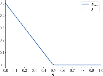
Figure 6: The graph of the entanglement negativity $E_{\text{neg}}$ of Werner states $\bm{\rho}_{q}^{\text{Werner}}$ parameterized by $q\in[0,1]$ against the parameter $q$ is plotted by the light blue solid line, and the graph of the atemporality, $f$ is plotted by the blue dashed line.

See 7

Proof.

Since $\mathbf{R}_{AB}$ is a forward temporal PDO with its first marginal being $\bm{\rho}_{A}$ and its pseudo-channel being $\mathcal{U}$, we have

$$\mathbf{R}_{AB}=\left(\mathcal{I}\otimes\mathcal{U}\right)\left\{\bm{\rho}_{A}\otimes\frac{\mathbf{I}}{2},\mathbf{S}\right\}.$$ (28)

Now, we consider its swapped PDO $\mathbf{R}^{\prime}_{BA}$, i.e., $\mathbf{R}^{\prime}=\mathbf{S}\mathbf{R}\mathbf{S}^{\dagger}$. We also note that $\left\{\bm{\rho}_{A}\otimes\frac{\mathbf{I}}{2},\mathbf{S}\right\}=\left\{\frac{\mathbf{I}}{2}\otimes\bm{\rho}_{A},\mathbf{S}\right\}$:

$$\left\{\frac{\mathbf{I}}{2}\otimes\bm{\rho}_{A},\mathbf{S}\right\} = \left(\frac{\mathbf{I}}{2}\otimes\bm{\rho}_{A}\right)\mathbf{S}+\mathbf{S}\left(\frac{\mathbf{I}}{2}\otimes\bm{\rho}_{A}\right)$$ (29)

$$= \mathbf{S}\mathbf{S}\left(\frac{\mathbf{I}}{2}\otimes\bm{\rho}_{A}\right)\mathbf{S}+\mathbf{S}\left(\frac{\mathbf{I}}{2}\otimes\bm{\rho}_{A}\right)\mathbf{S}\mathbf{S}$$ (30)

$$= \mathbf{S}\left(\bm{\rho}_{A}\otimes\frac{\mathbf{I}}{2}\right)+\left(\bm{\rho}_{A}\otimes\frac{\mathbf{I}}{2}\right)\mathbf{S}$$ (31)

$$= \left\{\bm{\rho}_{A}\otimes\frac{\mathbf{I}}{2},\mathbf{S}\right\},$$ (32)

where we used $\mathbf{S}\mathbf{S}=\mathbf{I}$. The swapped PDO $\mathbf{R}^{\prime}$ can be written as $\mathbf{R}^{\prime}=\left(\mathcal{U}\otimes\mathcal{I}\right)\left\{\frac{\mathbf{I}}{2}\otimes\bm{\rho}_{A},\mathbf{S}\right\}$ by switching $A$ and $B$ as the action of the swap operation on $\mathbf{R}$. By using the above observation, we have $\mathbf{R}^{\prime}=\left(\mathcal{U}\otimes\mathcal{I}\right)\left\{\bm{\rho}_{A}\otimes\frac{\mathbf{I}}{2},\mathbf{S}\right\}$. Thus, we show that $\mathbf{R}^{\prime}$ can be expressed as follows:

$$\mathbf{R}^{\prime} = \left(\mathcal{U}\otimes\mathcal{I}\right)\left\{\bm{\rho}_{A}\otimes\frac{\mathbf{I}}{2},\mathbf{S}\right\}$$ (33)

$$= \left\{\left(\mathcal{U}\otimes\mathcal{I}\right)\left(\bm{\rho}_{A}\otimes\frac{\mathbf{I}}{2}\right),\left(\mathcal{U}\otimes\mathcal{I}\right)\left(\mathbf{S}\right)\right\}$$ (34)

$$= \left\{\mathcal{U}\left(\bm{\rho}_{A}\right)\otimes\frac{\mathbf{I}}{2},\left(\mathcal{I}\otimes\mathcal{U}^{\dagger}\right)\left(\mathbf{S}\right)\right\}$$ (35)

$$= \left(\mathcal{I}\otimes\mathcal{U}^{\dagger}\right)\left\{\mathcal{U}\left(\bm{\rho}_{A}\right)\otimes\frac{\mathbf{I}}{2},\mathbf{S}\right\}.$$ (36)

The third equation holds due to the fact that $(\mathbf{I}\otimes\mathbf{M})\ket{\Phi^{+}}=(\mathbf{M}^{T}\otimes\mathbf{I})\ket{\Phi^{+}}$ for any linear operator $\mathbf{M}$, where $\ket{\Phi^{+}}$ denotes the maximally entangled state and $(\cdot)^{T}$ denotes the transpose map.

Hence we conclude that $\mathbf{R}_{AB}$ is reverse temporal with the adjoint channel $\mathcal{U}^{\dagger}$ as its reverse pseudo-channel and $\mathcal{U}(\bm{\rho})$ as its associated initial state. ∎

See 8

Fig. 7 shows the asymmetry of atemporality on randomly sampled density operators. The discrepancy between forward atemporality $\overrightarrow{f}$ and reverse atemporality $\overleftarrow{f}$ is plotted outside of the x-y line. In particular, those on the y-axis indicate the existence of temporal PDOs from the point of view that the system $A$ occurs before the system $B$ but they are not temporal in the reverse point of view. This shows that the forward atemporality does not imply the reverse atemporality, and vice versa.

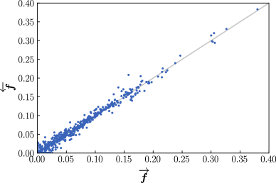
Figure 7: The graph of $\overrightarrow{f}$ against $\overleftarrow{f}$ for 1000 uniformly random PDO $\mathbf{R}\in\mathcal{S}$. The grey line represents the $x=y$ line.

See 9

Fig. 8 is the graph of entanglement negativity [20] against atemporality plotted on randomly sampled density operators.

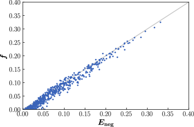
Figure 8: The graph of the entanglement negativity $E_{\text{neg}}$ against the atemporality $f$ for 1000 uniformly random PDO $\mathbf{R}\in\mathcal{S}$. The grey line represents the $x=y$ line.

Supplementary Information B Proofs of technical results

Imagine that Alice and Bob have qubit systems, $A$ and $B$, respectively, and they had been temporally distributed where measurements on the system $A$ occurs before measurements on the system $B$, namely, the system $A$ is initially prepared in some state $\bm{\rho}_{A}$ and the system $B$ is the result of acting some physical time evolution $\mathcal{E}$ on the post-measurement state of the qubit $A$. Each round, Alice and Bob implement Pauli measurements in their choices $a,b$ of basis. In this scenario, the joint probability $\Pr(xy|ab)$ to obtain the measurement outcome $x,y$ is given by

$$\Pr(xy|ab)=\tr[\mathcal{E}\left(\bm{\Pi}_{x|a}\bm{\rho}_{A}\bm{\Pi}_{x|a}\right)\bm{\Pi}_{y|b}\bigr{]},$$ (37)

where $\bm{\Pi}_{x|a},\bm{\Pi}_{y|b}$ denotes the projection operator to $x,y$ of the Pauli operator $\bm{\sigma}_{a},\bm{\sigma}_{b}$, respectively.

According to the known results in [6, 14], it was shown that the corresponding PDO $\mathbf{R}_{AB}$ can be written by its associated initial state $\bm{\rho}_{A}$ of the system $A$ and its associated physical time evolution $\mathcal{E}:A\to B$ as

$$\mathbf{R}_{AB}=\left(\mathcal{I}\otimes\mathcal{E}\right)\mathbf{K},\qquad\mathrm{where}\,\,\mathbf{K}=\left\{\bm{\rho}_{A}\otimes\frac{\mathbf{I}}{2},\mathbf{S}\right\}.$$ (38)

Here $\mathbf{S}$ denotes the swap operator, i.e., $\mathbf{S}\equiv\frac{1}{2}\sum_{k=0}^{3}\bm{\sigma}_{k}\otimes\bm{\sigma}_{k}$, and the curly bracket denotes the anti-commutator, i.e., $\{\mathbf{A},\mathbf{B}\}=\mathbf{A}\mathbf{B}+\mathbf{B}\mathbf{A}$. For notational shorthand, we denote $\left\{\bm{\rho}_{A}\otimes\frac{\mathbf{I}}{2},\mathbf{S}\right\}$ by $\mathbf{K}$ in what follows. Note that $\bm{\rho}_{A}$ is a density operator that $\bm{\rho}_{A}=\tr_{B}\mathbf{R}_{AB}$ and $\mathcal{E}$ is a completely positive (CP) and trace-preserving (TP) map.

Indeed, from Eq. (37), we have expectation values $\expectationvalue{\bm{\sigma}_{a},\bm{\sigma}_{b}}$:

$$\expectationvalue{\bm{\sigma}_{a},\bm{\sigma}_{b}} \equiv \sum_{xy}xy\cdot\Pr(xy|ab)$$ (39)

$$= \sum_{xy}xy\cdot\tr\left[\mathcal{E}(\bm{\Pi}_{x|a}\bm{\rho}_{A}\bm{\Pi}_{x|a})\bm{\Pi}_{y|b}\right]$$ (40)

$$= \tr[\mathcal{E}\left(\sum_{x}x\cdot\bm{\Pi}_{x|a}\bm{\rho}_{A}\bm{\Pi}_{x|a}\right)\left(\sum_{y}y\cdot\bm{\Pi}_{y|b}\right)\bigr{]}$$ (41)

$$= \tr\left[\mathcal{E}\left(\frac{1}{2}\left\{\bm{\rho}_{A},\bm{\sigma}_{a}\right\}\right)\bm{\sigma}_{b}\right].$$ (42)

The last equation holds due to the fact that $\bm{\sigma}_{a}=\sum_{x}x\cdot\bm{\Pi}_{x|a}$ and $\bm{\Pi}_{x|a}=\frac{1}{2}\left(\mathbf{I}+x\bm{\sigma}_{a}\right)$. By using $\bm{\Pi}_{x|a}=\frac{1}{2}\left(\mathbf{I}+x\bm{\sigma}_{a}\right)$, we indeed have $\sum_{x=-1,+1}x\cdot\bm{\Pi}_{x|a}\bm{\rho}_{A}\bm{\Pi}_{x|a}=\frac{1}{2}(\bm{\rho}_{A}\bm{\sigma}_{a}+\bm{\sigma}_{a}\bm{\rho}_{A})$ (recall that the curly bracket here represents the anti-commutator). Then it is led to Eq. 38 by virtue of the cyclic property of the trace and the fact that $\frac{1}{2}\sum_{k}\tr\left[\left\{\bm{\rho}_{A},\bm{\sigma}_{a}\right\}\bm{\sigma}_{k}\right]\bm{\sigma}_{k}=\left\{\bm{\rho}_{A},\bm{\sigma}_{a}\right\}$:

$$\mathbf{R}_{AB} \equiv \frac{1}{4}\sum_{ab}\expectationvalue{\bm{\sigma}_{a},\bm{\sigma}_{b}}\bm{\sigma}_{a}\otimes\bm{\sigma}_{b}$$ (43)

$$= \frac{1}{4}\sum_{ab}\tr[\mathcal{E}\left(\frac{1}{2}\left\{\bm{\rho}_{A},\bm{\sigma}_{a}\right\}\right)\bm{\sigma}_{b}\biggr{]}\bm{\sigma}_{a}\otimes\bm{\sigma}_{b}$$ (44)

$$= \frac{1}{8}\sum_{ab}\frac{1}{2}\sum_{k}\tr[\left\{\bm{\rho}_{A},\bm{\sigma}_{a}\right\}\bm{\sigma}_{k}\bigr{]}\cdot\tr[\mathcal{E}\left(\bm{\sigma}_{k}\right)\bm{\sigma}_{b}\bigr{]}\bm{\sigma}_{a}\otimes\bm{\sigma}_{b}$$ (45)

$$= \frac{1}{16}\sum_{ab}\sum_{k}\tr[\left\{\bm{\rho}_{A},\bm{\sigma}_{k}\right\}\bm{\sigma}_{a}\bigr{]}\cdot\tr[\mathcal{E}\left(\bm{\sigma}_{k}\right)\bm{\sigma}_{b}\bigr{]}\bm{\sigma}_{a}\otimes\bm{\sigma}_{b}$$ (46)

$$= \frac{1}{16}\sum_{k}\sum_{ab}\tr[\bigl{(}\left\{\bm{\rho}_{A},\bm{\sigma}_{k}\right\}\otimes\mathcal{E}\left(\bm{\sigma}_{k}\right)\bigr{)}\bm{\sigma}_{a}\otimes\bm{\sigma}_{b}\Bigr{]}\bm{\sigma}_{a}\otimes\bm{\sigma}_{b}$$ (47)

$$= \frac{1}{4}\sum_{k}\left\{\bm{\rho}_{A},\bm{\sigma}_{k}\right\}\otimes\mathcal{E}\left(\bm{\sigma}_{k}\right).$$ (48)

The original proof was provided in Appendix A of the literature [14]. Or equivalently, $\mathbf{R}_{AB}$ can be written as

$$\mathbf{R}_{AB} = \frac{1}{4}\sum_{ab}\tr\left[\frac{1}{2}\mathcal{E}\bigl{(}\left\{\bm{\rho}_{A},\bm{\sigma}_{a}\right\}\bigr{)}\bm{\sigma}_{b}\right]\bm{\sigma}_{a}\otimes\bm{\sigma}_{b}$$ (49)

$$= \frac{1}{4}\sum_{a}\bm{\sigma}_{a}\otimes\left(\frac{1}{2}\sum_{b}\tr[\mathcal{E}\bigl{(}\left\{\bm{\rho}_{A},\bm{\sigma}_{a}\right\}\bigr{)}\bm{\sigma}_{b}\Bigr{]}\bm{\sigma}_{b}\right)$$ (50)

$$= \frac{1}{4}\sum_{a}\bm{\sigma}_{a}\otimes\mathcal{E}\bigl{(}\left\{\bm{\rho}_{A},\bm{\sigma}_{a}\right\}\bigr{)}$$ (51)

$$= \left(\frac{1}{4}\sum_{a\neq 0}\bm{\sigma}_{a}\otimes\mathcal{E}\bigl{(}\left\{\bm{\rho}_{A},\bm{\sigma}_{a}\right\}\bigr{)}\right)+\left(\frac{\mathbf{I}}{2}\otimes\mathcal{E}\left(\bm{\rho}_{A}\right)\right)$$ (52)

$$= \left(\frac{1}{4}\sum_{a\neq 0}\bm{\sigma}_{a}\otimes\mathcal{E}\bigl{(}\bm{\sigma}_{a}+\tr[\bm{\rho}_{A}\bm{\sigma}_{a}]\mathbf{I}\right)\bigr{)}+\left(\frac{\mathbf{I}}{2}\otimes\mathcal{E}\left(\bm{\rho}_{A}\right)\right)$$ (53)

$$= \left(\frac{1}{4}\sum_{a\neq 0}\bm{\sigma}_{a}\otimes\mathcal{E}\left(\bm{\sigma}_{a}\right)+\frac{1}{4}\sum_{a\neq 0}\tr[\bm{\rho}_{A}\bm{\sigma}_{a}]\bm{\sigma}_{a}\otimes\mathcal{E}\left(\mathbf{I}\right)\right)+\left(\frac{\mathbf{I}}{2}\otimes\mathcal{E}\left(\bm{\rho}_{A}\right)\right)$$ (54)

$$= \left(\frac{1}{4}\sum_{a}\bm{\sigma}_{a}\otimes\mathcal{E}\left(\bm{\sigma}_{a}\right)\right)+\left(\bm{\rho}_{A}-\frac{\mathbf{I}}{2}\right)\otimes\mathcal{E}\left(\frac{\mathbf{I}}{2}\right)+\frac{\mathbf{I}}{2}\otimes\mathcal{E}\left(\bm{\rho}_{A}-\frac{\mathbf{I}}{2}\right).$$ (55)

In the fifth equation, we used the following:

$$\forall a\in\left\{1,2,3\right\},\quad\left\{\bm{\rho}_{A},\bm{\sigma}_{a}\right\} = \frac{1}{2}\sum_{k}\tr\left[\bm{\rho}_{A}\bm{\sigma}_{k}\right]\left\{\bm{\sigma}_{k},\bm{\sigma}_{a}\right\},$$ (56)

$$= \bm{\sigma}_{a}+\frac{1}{2}\sum_{k\neq 0}\tr\left[\bm{\rho}_{A}\bm{\sigma}_{k}\right]\left\{\bm{\sigma}_{k},\bm{\sigma}_{a}\right\},$$ (57)

$$= \bm{\sigma}_{a}+\frac{1}{2}\sum_{k\neq 0}\tr\left[\bm{\rho}_{A}\bm{\sigma}_{k}\right]\left(2\delta_{k,a}\mathbf{I}\right),$$ (58)

$$= \bm{\sigma}_{a}+\tr[\bm{\rho}_{A}\bm{\sigma}_{a}]\mathbf{I},$$ (59)

where $\delta_{i,j}$ denotes the Kronecker delta.

In summary, we have three different versions of representing a PDO, which we will vastly make use of:

$$\bullet\quad\mathbf{R}_{AB} = \frac{1}{4}\sum_{a}\bm{\sigma}_{a}\otimes\mathcal{E}\bigl{(}\left\{\bm{\rho}_{A},\bm{\sigma}_{a}\right\}\bigr{)},$$ (60)

$$\bullet\quad\mathbf{R}_{AB} = \left(\frac{1}{4}\sum_{a\neq 0}\bm{\sigma}_{a}\otimes\mathcal{E}\bigl{(}\bm{\sigma}_{a}+\tr[\bm{\rho}_{A}\bm{\sigma}_{a}]\mathbf{I}\bigr{)}\right)+\frac{\mathbf{I}}{2}\otimes\mathcal{E}\left(\bm{\rho}_{A}\right),$$ (61)

$$\bullet\quad\mathbf{R}_{AB} = \left(\frac{1}{4}\sum_{a}\bm{\sigma}_{a}\otimes\mathcal{E}\left(\bm{\sigma}_{a}\right)\right)+\left(\bm{\rho}_{A}-\frac{\mathbf{I}}{2}\right)\otimes\mathcal{E}\left(\frac{\mathbf{I}}{2}\right)+\frac{\mathbf{I}}{2}\otimes\mathcal{E}\left(\bm{\rho}_{A}-\frac{\mathbf{I}}{2}\right).$$ (62)

We will use different representations specific to respective contexts.

1 provides a way to apply the above construction to general cases; any PDOs can be represented as though its subsystems were temporally distributed.

See 1

Proof.

Recall that a forward pseudo-channel of a 2-qubit PDO $\mathbf{R}_{AB}$ is defined as a linear trace preserving map $\Lambda$ that satisfies

$$\mathbf{R}_{AB}=\left(\mathcal{I}_{A}\otimes\Lambda\right)\mathbf{K},\qquad\mathrm{where}\,\,\mathbf{K}=\left\{\bm{\rho}_{A}\otimes\frac{\mathbf{I}}{2},\mathbf{S}\right\}\,\,\mathrm{and}\,\,\bm{\rho}_{A}=\tr_{B}\mathbf{R}_{AB}.$$ (63)

Observe that if there exists such map satisfying above equation, it follows that

$$\tr_{A}\bigl{[}\left(\bm{\sigma}_{i}\otimes\mathbf{I}\right)\mathbf{R}_{AB}\bigr{]}=\Lambda\bigl{(}\left\{\bm{\rho}_{A},\bm{\sigma}_{i}\right\}\bigr{)}.$$ (64)

Let $\mathbf{R}_{AB}$ be any PDO such that $\mathbf{R}_{AB}=\frac{1}{4}\sum_{i,j}r_{ij}\bm{\sigma}_{i}\otimes\bm{\sigma}_{j}$ for $r_{ij}\in\mathbb{R}$ where $r_{00}=1$. Based on the above observation, we can construct a linear (Hermiticity-preserving) map with scalar multiplication as

$$\Lambda\bigl{(}\left\{\bm{\rho}_{A},\bm{\sigma}_{i}\right\}\bigr{)} \equiv \tr_{A}\bigl{[}\left(\bm{\sigma}_{i}\otimes\mathbf{I}\right)\mathbf{R}_{AB}\bigr{]}$$ (65)

$$= \sum_{k}r_{ik}\bm{\sigma}_{k},$$ (66)

where $\bm{\rho}_{A}$ denotes the first marginal of $\mathbf{R}_{AB}$, i.e., $\bm{\rho}_{A}\equiv\tr_{B}\mathbf{R}_{AB}$.

We will prove that, (1) $\Lambda$ indeed satisfies that $\mathbf{R}_{AB}=(\mathcal{I}\otimes\Lambda)\mathbf{K}$, (2) $\Lambda$ is well-defined, and that (3) $\Lambda$ is a trace-preserving map.

(1) Firstly, we show that the map $\Lambda$ satisfies that $\mathbf{R}_{AB}=(\mathcal{I}\otimes\Lambda)\mathbf{K}$. As Pauli operators and the identity operator span the space of Hermitian operators and $\mathbf{R}_{AB}$ is a Hermitian operator, we can instead show that $\tr[\bm{\sigma}_{i}\otimes\bm{\sigma}_{j}\mathbf{R}_{AB}]=\tr\left[\bm{\sigma}_{i}\otimes\bm{\sigma}_{j}(\mathcal{I}\otimes\Lambda)\mathbf{K}\right]$ for any $\bm{\sigma}_{i},\bm{\sigma}_{j}$. Thus we have

$$\tr\left[\bm{\sigma}_{i}\otimes\bm{\sigma}_{j}(\mathcal{I}\otimes\Lambda)\mathbf{K}\right] = \frac{1}{4}\sum_{k}\tr[\bm{\sigma}_{i}\left\{\bm{\rho}_{A},\bm{\sigma}_{k}\right\}\bigr{]}\cdot\tr[\bm{\sigma}_{j}\Lambda\left(\bm{\sigma}_{k}\right)\bigr{]}$$ (67)

$$= \frac{1}{4}\sum_{k}\tr[\left\{\bm{\sigma}_{i},\bm{\rho}_{A}\right\}\bm{\sigma}_{k}\bigr{]}\cdot\tr[\bm{\sigma}_{j}\Lambda\left(\bm{\sigma}_{k}\right)\bigr{]}$$ (68)

$$= \frac{1}{2}\tr\left[\bm{\sigma}_{j}\cdot\Lambda\left(\frac{1}{2}\sum_{k}\tr[\bm{\sigma}_{k}\left\{\bm{\rho}_{A},\bm{\sigma}_{i}\right\}\bigr{]}\bm{\sigma}_{k}\right)\right]$$ (69)

$$= \frac{1}{2}\tr[\bm{\sigma}_{j}\cdot\Lambda\bigl{(}\left\{\bm{\rho}_{A},\bm{\sigma}_{i}\right\}\bigr{)}\Bigr{]}$$ (70)

$$= \frac{1}{2}\tr\left[\bm{\sigma}_{j}\sum_{k}r_{ik}\bm{\sigma}_{k}\right]$$ (71)

$$= \frac{1}{2}\sum_{k}r_{ik}\tr\left[\bm{\sigma}_{j}\bm{\sigma}_{k}\right]$$ (72)

$$= \frac{1}{2}\sum_{k}r_{ik}2\delta_{j,k}=r_{ij}=\tr[\bm{\sigma}_{i}\otimes\bm{\sigma}_{j}\mathbf{R}].$$ (73)

Recall that $\mathbf{K}=\frac{1}{4}\sum_{k}\{\bm{\rho}_{A},\bm{\sigma}_{k}\}\otimes\bm{\sigma}_{k}$. The fourth equation holds because Pauli operators and the identity operator form the complete basis of the space of all linear operators and thus $\left\{\bm{\rho}_{A},\bm{\sigma}_{i}\right\}=\frac{1}{2}\sum_{k}\tr[\bm{\sigma}_{k}\left\{\bm{\rho}_{A},\bm{\sigma}_{i}\right\}]\bm{\sigma}_{k}$. By definition of the map $\Lambda$, the fifth equation follows.

(2) Secondly, we will show that the map $\Lambda$ is a well-defined map on the space spanned by $\left\{\bm{\rho}_{A},\bm{\sigma}_{i}\right\},~{}\forall i$. To verify whether the map $\Lambda$ is well defined on such space, we need to prove that if $\left\{\bm{\rho}_{A},\bm{\sigma}_{i_{1}}\right\}=\left\{\bm{\rho}_{A},\bm{\sigma}_{i_{2}}\right\}$, then $\Lambda\left(\left\{\bm{\rho}_{A},\bm{\sigma}_{i_{1}}\right\}\right)=\Lambda\left(\left\{\bm{\rho}_{A},\bm{\sigma}_{i_{2}}\right\}\right)$. Assume that $\left\{\bm{\rho}_{A},\bm{\sigma}_{i_{1}}\right\}=\left\{\bm{\rho}_{A},\bm{\sigma}_{i_{2}}\right\}$.

(2a) If $i_{1}\neq 0$ and $i_{2}\neq 0$,

$$\left\{\bm{\rho}_{A},\bm{\sigma}_{i_{1}}\right\}=\left\{\bm{\rho}_{A},\bm{\sigma}_{i_{2}}\right\} \Rightarrow \sum_{j}\frac{r_{j,0}}{2}\left\{\bm{\sigma}_{j},\bm{\sigma}_{i_{1}}\right\}=\sum_{j}\frac{r_{j,0}}{2}\left\{\bm{\sigma}_{j},\bm{\sigma}_{i_{2}}\right\}$$ (74)

$$\Rightarrow \bm{\sigma}_{i_{1}}+r_{i_{1},0}\mathbf{I}=\bm{\sigma}_{i_{2}}+r_{i_{2},0}\mathbf{I}$$ (75)

Note that $\bm{\rho}_{A}=\sum_{j}\dfrac{r_{j,0}}{2}\bm{\sigma}_{j}$ and $r_{00}=1$. Multiplying both hand sides of Eq. (75) by $\bm{\sigma}_{i_{1}}$ and taking a trace of the entire term, we have $i_{1}=i_{2}$ because $2=\tr[\bm{\sigma}_{i_{1}}\bm{\sigma}_{i_{2}}]$. It follows that

$$\Lambda\left(\left\{\bm{\rho}_{A},\bm{\sigma}_{i_{1}}\right\}\right) = \Lambda\left(\left\{\bm{\rho}_{A},\bm{\sigma}_{i_{2}}\right\}\right).$$ (76)

(2b) Otherwise, without loss of generality, let $i_{1}=0$.

It is trivial that if $i_{2}=i_{1}=0$, $\Lambda\left(\left\{\bm{\rho}_{A},\bm{\sigma}_{i_{1}}\right\}\right)=\Lambda\left(\left\{\bm{\rho}_{A},\bm{\sigma}_{i_{2}}\right\}\right)$. Now assume that $i_{2}\neq 0$, and see if the equation $\Lambda\left(\left\{\bm{\rho}_{A},\bm{\sigma}_{i_{1}}\right\}\right)=\Lambda\left(\left\{\bm{\rho}_{A},\bm{\sigma}_{i_{2}}\right\}\right)$ still holds. The initial assumption of $\left\{\bm{\rho}_{A},\bm{\sigma}_{i_{1}}\right\}=\left\{\bm{\rho}_{A},\bm{\sigma}_{i_{2}}\right\}$ implies that $\bm{\rho}_{A}=\frac{1}{2}(\mathbf{I}+\bm{\sigma}_{i_{2}})$. Let $\mathbf{\Pi}_{x|a}$ denote the projector of a Pauli operator $\bm{\sigma}_{a}$ associated with its eigenvalue $x$, that is, $\bm{\sigma}_{a}=\sum_{x=\pm 1}x\mathbf{\Pi}_{x|a}$, and we note that $\mathbf{\Pi}_{x|a}=\frac{1}{2}(\mathbf{I}+x\bm{\sigma}_{a})$. Thus, $\bm{\rho}_{A}$ can be rewritten as $\bm{\rho}_{A}=\mathbf{\Pi}_{+1|i_{2}}$, and furthermore

$$\tr_{A}[\left(\mathbf{\Pi}_{-1|i_{2}}\otimes\mathbf{I}\right)\mathbf{R}_{AB}] = \frac{1}{4}\tr\left[\left\{\bm{\rho}_{A},\bm{\sigma}_{k}\right\}\mathbf{\Pi}_{-1|i_{2}}\right]\Lambda(\bm{\sigma}_{k})$$ (77)

$$= \frac{1}{4}\tr\left[\left\{\bm{\rho}_{A},\mathbf{\Pi}_{-1|i_{2}}\right\}\bm{\sigma}_{k}\right]\Lambda(\bm{\sigma}_{k})$$ (78)

$$= \mathbf{0},$$ (79)

where $\mathbf{0}$ denotes the zero operator whose elements are all zero. The second equality holds due to the cyclic property of the trace, and the last equality holds because $\mathbf{\Pi}_{+1|i_{2}}\cdot\mathbf{\Pi}_{-1|i_{2}}=\mathbf{\Pi}_{-1|i_{2}}\cdot\mathbf{\Pi}_{+1|i_{2}}=\mathbf{0}$. Together with the fact that $\mathbf{\Pi}_{-1|i_{2}}=\frac{1}{2}(\mathbf{I}-\bm{\sigma}_{a})$, this leads us to $\tr_{A}\mathbf{R}=\tr_{A}[\left(\bm{\sigma}_{i_{2}}\otimes\mathbf{I}\right)\mathbf{R}]$, i.e., $\sum_{k}r_{0,k}\bm{\sigma}_{k}=\sum_{k}r_{i_{2},k}\bm{\sigma}_{k}$:

$$\mathbf{0}=\tr_{A}[\left(\mathbf{\Pi}_{-1|i_{2}}\otimes\mathbf{I}\right)\mathbf{R}_{AB}] \Leftrightarrow \mathbf{0}=\tr_{A}\left[\left(\frac{\mathbf{I}-\bm{\sigma}_{i_{2}}}{2}\otimes\mathbf{I}\right)\mathbf{R}_{AB}\right]$$ (80)

$$\Leftrightarrow \tr_{A}\mathbf{R}_{AB}=\tr_{A}\bigl{[}\left(\bm{\sigma}_{i_{2}}\otimes\mathbf{I}\right)\mathbf{R}_{AB}\bigr{]}.$$ (81)

By using $\sum_{k}r_{0,k}\bm{\sigma}_{k}=\sum_{k}r_{i_{2},k}\bm{\sigma}_{k}$, we have

$$\Lambda\bigl{(}\left\{\bm{\rho}_{A},\bm{\sigma}_{i_{1}}\right\}\bigr{)} = \Lambda\bigl{(}\left\{\bm{\rho}_{A},\bm{\sigma}_{0}\right\}\bigr{)}$$ (82)

$$= \sum_{k}r_{0,k}\bm{\sigma}_{k}$$ (83)

$$= \sum_{k}r_{i_{2},k}\bm{\sigma}_{k}$$ (84)

$$= \Lambda\bigl{(}\left\{\bm{\rho}_{A},\bm{\sigma}_{i_{2}}\right\}\bigr{)}.$$ (85)

(3) Lastly, we check if the map $\Lambda$ is trace-preserving: the trace of $\left\{\bm{\rho}_{A},\bm{\sigma}_{i}\right\}$ is given by

$$\tr\left\{\bm{\rho}_{A},\bm{\sigma}_{i}\right\} = 2\tr[\bm{\rho}_{A}\bm{\sigma}_{i}]$$ (86)

$$= \sum_{j}r_{j,0}\tr[\bm{\sigma}_{j}\bm{\sigma}_{i}]$$ (87)

$$= 2r_{i,0},$$ (88)

and the trace of $\Lambda\bigl{(}\left\{\bm{\rho}_{A},\bm{\sigma}_{i}\right\}\bigr{)}$ is given by

$$\tr\Lambda\bigl{(}\left\{\bm{\rho}_{A},\bm{\sigma}_{i}\right\}\bigr{)} = \sum_{k}r_{ik}\tr\bm{\sigma}_{k}$$ (89)

$$= \sum_{k}r_{i,k}2\delta_{k,0}$$ (90)

$$= 2r_{i,0}.$$ (91)

We have verified that the map $\Lambda$ is trace-preserving by observing that $\tr\left\{\bm{\rho}_{A},\bm{\sigma}_{i}\right\}=\tr\Lambda(\left\{\bm{\rho}_{A},\bm{\sigma}_{i}\right\})$ for $i$.

In a very similar way, we can prove the existence of a reverse pseudo-channel, its well-definedness, and its trace-preserving property.

Hence, we conclude that for any PDO $\mathbf{R}_{AB}$ there exists a forward pseudo-channel and a reverse pseudo-channel. ∎

Although we could prove that the map, defined as Eq. (66), is trace-preserving (TP), what was proven is that it is TP on the domain that $\{\bm{\rho}_{A},\bm{\sigma}_{i}\}_{i}$ spans (here the curly bracket is the normal bracket that is used to represent sets). Thus, the condition in Eq. (66) is equivalent to trace-preserving requirement on the domain of all linear operators, if $\bm{\rho}_{A}$ has full rank. It is because $\{\bm{\rho}_{A},\bm{\sigma}_{i}\}_{i}$ spans the set of all linear operators, if $\bm{\rho}_{A}$ has full rank. Thus, for the cases where $\bm{\rho}_{A}$ does not have full rank, we impose the condition of trace-preserving in addition to Eq. (66).

The following theorem underlies Algorithm 1 in the main text.

See 2

Proof.

Let $\mathbf{R}_{AB}$ be a PDO and $\bm{\rho}_{A}$ its first marginal, i.e., $\bm{\rho}_{A}\equiv\tr_{B}\mathbf{R}_{AB}$. As it is clear that we are only concerned a forward pseudo-channel in this proof, we omit the symbol $\rightarrow$ from the pseudo-channels for brevity.

(1) Suppose that $\bm{\rho}_{A}$ has full rank. Then $\bm{\rho}_{A}$ is invertible, so there exists its inverse $\bm{\rho}_{A}^{-1}$. By 1, $\mathbf{R}_{AB}$ has the unique pseudo-channel $\Lambda$ that satisfies $\mathbf{R}_{AB}=(\mathcal{I}\otimes\Lambda)\mathbf{K}=\frac{1}{4}\sum_{k}\left\{\bm{\rho}_{A},\bm{\sigma}_{k}\right\}\otimes\Lambda(\bm{\sigma}_{k})$. In turn, we show that the Choi state $\bm{{\mathchoice{\raisebox{0.0pt}{$\displaystyle\chi$}}{\raisebox{0.0pt}{$\textstyle\chi$}}{\raisebox{0.0pt}{$\scriptstyle\chi$}}{\raisebox{0.0pt}{$\scriptscriptstyle\chi$}}}}_{\Lambda}$ of this unique pseudo-channel $\Lambda$ is given by $\bm{{\mathchoice{\raisebox{0.0pt}{$\displaystyle\chi$}}{\raisebox{0.0pt}{$\textstyle\chi$}}{\raisebox{0.0pt}{$\scriptstyle\chi$}}{\raisebox{0.0pt}{$\scriptscriptstyle\chi$}}}}_{\Lambda}=\left(T\otimes\mathcal{I}\right)\left(\mathbf{R}_{AB}-\mathbf{L}_{AB}\right)$, where

$$\begin{aligned} \mathbf{L}_{AB}\equiv\left(\bm{\rho}_{A}-\frac{\mathbf{I}}{2}\right)\otimes\tr_{A}\left[\left(\frac{1}{2}\bm{\rho}_{A}^{-1}\otimes\mathbf{I}\right)\mathbf{R}_{AB}\right]+\frac{\mathbf{I}}{2}\otimes\tr_{A}\left[\left((\mathbf{I}-\frac{1}{2}\bm{\rho}_{A}^{-1})\otimes\mathbf{I}\right)\mathbf{R}_{AB}\right].\end{aligned}$$ (92)

Firstly, we show that

$$\tr_{A}\Bigl{[}\left(\bm{\rho}_{A}^{-1}\otimes\mathbf{I}\right)\mathbf{R}_{AB}\Bigr{]}=\Lambda(\mathbf{I})$$ (93)

and

$$\tr_{A}\mathbf{R}_{AB}=\Lambda(\bm{\rho}_{A}),$$ (94)

then it follows that

$$\mathbf{L}_{AB}=\left(\bm{\rho}_{A}-\frac{\mathbf{I}}{2}\right)\otimes\Lambda\left(\frac{\mathbf{I}}{2}\right)+\frac{\mathbf{I}}{2}\otimes\Lambda\left(\bm{\rho}_{A}-\frac{\mathbf{I}}{2}\right).$$ (95)

Indeed, Eq. (93) and Eq. (94) hold:

$$\tr_{A}\left[\left(\bm{\rho}_{A}^{-1}\otimes\mathbf{I}\right)\mathbf{R}_{AB}\right] = \tr_{A}\left[\left(\bm{\rho}_{A}^{-1}\otimes\mathbf{I}\right)\left(\frac{1}{4}\sum_{k}\{\bm{\rho}_{A},\bm{\sigma}_{k}\}\otimes\Lambda(\bm{\sigma}_{k})\right)\right]$$ (96)

$$= \frac{1}{4}\sum_{k}\tr\left[\bm{\rho}_{A}^{-1}\{\bm{\rho}_{A},\bm{\sigma}_{k}\})\right]\Lambda(\bm{\sigma}_{k})$$ (97)

$$= \frac{1}{4}\sum_{k}2\tr[\bm{\sigma}_{k}]\Lambda(\bm{\sigma}_{k})$$ (98)

$$= \frac{1}{2}\sum_{k}2\delta_{k,0}\Lambda(\bm{\sigma}_{k})$$ (99)

$$= \Lambda(\mathbf{I}),$$ (100)

and

$$\tr_{A}\mathbf{R}_{AB} = \tr_{A}\left[\frac{1}{4}\sum_{k}\{\bm{\rho}_{A},\bm{\sigma}_{k}\}\otimes\Lambda(\bm{\sigma}_{k})\right]$$ (101)

$$= \sum_{k}\frac{\tr[\bm{\rho}_{A}\bm{\sigma}_{k}]}{2}\Lambda(\bm{\sigma}_{k})$$ (102)

$$= \Lambda\left(\sum_{k}\frac{\tr[\bm{\rho}_{A}\bm{\sigma}_{k}]}{2}\bm{\sigma}_{k}\right)$$ (103)

$$= \Lambda(\bm{\rho}_{A}).$$ (104)

Thus, we have $\mathbf{L}_{AB}=\left(\bm{\rho}_{A}-\frac{\mathbf{I}}{2}\right)\otimes\Lambda\left(\frac{\mathbf{I}}{2}\right)+\frac{\mathbf{I}}{2}\otimes\Lambda\left(\bm{\rho}_{A}-\frac{\mathbf{I}}{2}\right)$. Now let us recall Eq. (62) that a PDO $\mathbf{R}_{AB}$ can be written with its pseudo-channel $\Lambda$ and its marginal $\bm{\rho}_{A}$ as

$$\mathbf{R}_{AB}=\left(\frac{1}{4}\sum_{a}\bm{\sigma}_{a}\otimes\Lambda\left(\bm{\sigma}_{a}\right)\right)+\left(\bm{\rho}_{A}-\frac{\mathbf{I}}{2}\right)\otimes\Lambda\left(\frac{\mathbf{I}}{2}\right)+\frac{\mathbf{I}}{2}\otimes\Lambda\left(\bm{\rho}_{A}-\frac{\mathbf{I}}{2}\right).$$ (105)

Namely, we have

$$\mathbf{R}_{AB}=\bm{{\mathchoice{\raisebox{0.0pt}{$\displaystyle\chi$}}{\raisebox{0.0pt}{$\textstyle\chi$}}{\raisebox{0.0pt}{$\scriptstyle\chi$}}{\raisebox{0.0pt}{$\scriptscriptstyle\chi$}}}}_{\Lambda}^{T_{A}}+\mathbf{L}_{AB},$$ (106)

where $(\cdot)^{T_{A}}$ denote the partial transpose on the first system $A$. Recall that the Choi state $\bm{{\mathchoice{\raisebox{0.0pt}{$\displaystyle\chi$}}{\raisebox{0.0pt}{$\textstyle\chi$}}{\raisebox{0.0pt}{$\scriptstyle\chi$}}{\raisebox{0.0pt}{$\scriptscriptstyle\chi$}}}}_{\Lambda}$ is defined as $\bm{{\mathchoice{\raisebox{0.0pt}{$\displaystyle\chi$}}{\raisebox{0.0pt}{$\textstyle\chi$}}{\raisebox{0.0pt}{$\scriptstyle\chi$}}{\raisebox{0.0pt}{$\scriptscriptstyle\chi$}}}}_{\Lambda}\equiv\frac{1}{4}\sum_{a}(\bm{\sigma}_{a})^{T}\otimes\Lambda\left(\bm{\sigma}_{a}\right)$, with the transpose map $(\cdot)^{T}$. We then observe that the Choi state $\bm{{\mathchoice{\raisebox{0.0pt}{$\displaystyle\chi$}}{\raisebox{0.0pt}{$\textstyle\chi$}}{\raisebox{0.0pt}{$\scriptstyle\chi$}}{\raisebox{0.0pt}{$\scriptscriptstyle\chi$}}}}_{\Lambda}$ of the pseudo-channel $\Lambda$ is obtained by $\mathbf{R}_{AB}^{T_{A}}-\mathbf{L}_{AB}^{T_{A}}$.

(2) Now suppose that $\bm{\rho}_{A}$ does not have full rank, that is, it is pure. The proof is divided into two parts: We show (2a) conditions that a pseudo-channel of $\mathbf{R}_{AB}$ must satisfy, (2b) that there are infinitely many pseudo-channels compatible with $\mathbf{R}_{AB}$, and (2c) how we can systematically find these pseudo-channels.

(2a) We recall Eq. (61) that $\mathbf{R}_{AB}$ can be written as

$$\mathbf{R}_{AB}=\left(\frac{1}{4}\sum_{a\neq 0}\bm{\sigma}_{a}\otimes\Lambda\left(\bm{\sigma}_{a}+\tr[\bm{\rho}_{A}\bm{\sigma}_{a}]\mathbf{I}\right)\right)+\frac{\mathbf{I}}{2}\otimes\Lambda\left(\bm{\rho}_{A}\right).$$ (107)

From this, we can derive four simultaneous equations that a pseudo-channel $\Lambda$ of $\mathbf{R}_{AB}$ must satisfy:

$$\begin{aligned} \forall k\in\left\{1,2,3\right\},\quad\tr_{A}\bigl{[}\left(\bm{\sigma}_{k}\otimes\mathbf{I}\right)\mathbf{R}_{AB}\bigr{]}&=\left(\frac{1}{4}\sum_{a\neq 0}\tr\left[\bm{\sigma}_{k}\bm{\sigma}_{a}\right]\Lambda\bigl{(}\bm{\sigma}_{a}+\tr[\bm{\rho}_{A}\bm{\sigma}_{a}]\mathbf{I}\bigr{)}\right)+\tr\left[\frac{\bm{\sigma}_{k}}{2}\right]\Lambda\left(\bm{\rho}_{A}\right)\\ &=\frac{1}{4}\sum_{a\neq 0}\left(2\delta_{k,a}\right)\cdot\Lambda\bigl{(}\bm{\sigma}_{a}+\tr[\bm{\rho}_{A}\bm{\sigma}_{a}]\mathbf{I}\bigr{)}\\ &=\frac{1}{2}\Lambda\bigl{(}\bm{\sigma}_{k}+\tr[\bm{\rho}_{A}\bm{\sigma}_{k}]\mathbf{I}\bigr{)},\end{aligned}$$ (108)

and

$$\begin{aligned} \tr_{A}\mathbf{R}_{AB}&=\left(\frac{1}{4}\sum_{a\neq 0}\tr\left[\bm{\sigma}_{a}\right]\cdot\Lambda\bigl{(}\bm{\sigma}_{a}+\tr[\bm{\rho}_{A}\bm{\sigma}_{a}]\mathbf{I}\bigr{)}\right)+\tr\left[\frac{\mathbf{I}}{2}\right]\Lambda\left(\bm{\rho}_{A}\right)\\ &=\Lambda\left(\bm{\rho}_{A}\right).\end{aligned}$$ (109)

Here we used $\tr[\bm{\sigma}_{i}\bm{\sigma}_{j}]=2\delta_{ij},~{}\forall i,j$ and the traceless property of Pauli operators. By rearranging Eqs. (108) and Eq. (109), we have the following equations as in Methods of the main text:

$$\Lambda (\mathbf{X})+\tr[\ket{\psi}\!\bra{\psi}\mathbf{X}\bigr{]}\Lambda(\mathbf{I})=2\tr_{A}\bigl{[}(\mathbf{X}\otimes\mathbf{I})\mathbf{R}_{AB}\bigr{]},$$ (110)

$$\Lambda (\mathbf{Y})+\tr[\ket{\psi}\!\bra{\psi}\mathbf{Y}\bigr{]}\Lambda(\mathbf{I})=2\tr_{A}\bigl{[}(\mathbf{Y}\otimes\mathbf{I})\mathbf{R}_{AB}\bigr{]},$$ (111)

$$\Lambda (\,\mathbf{Z})+\tr[\ket{\psi}\!\bra{\psi}\,\mathbf{Z}\bigr{]}\Lambda(\mathbf{I})=2\tr_{A}\bigl{[}(\,\mathbf{Z}\otimes\mathbf{I})\mathbf{R}_{AB}\bigr{]},$$ (112)

$$\Lambda \left(\ket{\psi}\!\bra{\psi}\right)=\tr_{A}\mathbf{R}_{AB},$$ (113)

where we denote $\bm{\rho}_{A}$ by $\ket{\psi}\!\bra{\psi}$ for some unit vector $\psi$, because it is pure.

(2b) As the Pauli operators and the identity operator form a complete basis for the space of linear operators, the left hand side of the last equation can be expanded in this basis $\Lambda(\bm{\sigma}_{i})$’s. Consequently, the last equation become

$$\frac{1}{2}\sum_{i}\tr[\ket{\psi}\!\bra{\psi}\bm{\sigma}_{i}\bigr{]}\Lambda(\bm{\sigma}_{i})=\tr_{A}\mathbf{R}_{AB}.$$ (114)

To solve the above simultaneous equations, we plug Eqs. (110,111,112) into Eq. (114). Then we observe that Eq. (114) is redundant, that is, in the rank-deficient cases, we have only three simultaneous equations and four unknown operators $\Lambda(\mathbf{X}),\Lambda(\mathbf{Y}),\Lambda(\mathbf{Z}),$ and $\Lambda(\mathbf{I})$:

$$\frac{1}{2}\Lambda(\mathbf{I})+\frac{1}{2}\left(\sum_{i\neq 0}\tr[\ket{\psi}\!\bra{\psi}\bm{\sigma}_{i}\bigr{]}\Bigl{(}2\tr_{A}\bigl{[}\left(\bm{\sigma}_{i}\otimes\mathbf{I}\right)\mathbf{R}_{AB}\bigr{]}-\tr[\ket{\psi}\!\bra{\psi}\bm{\sigma}_{i}\bigr{]}\Lambda\left(\mathbf{I}\right)\Bigr{)}\right)=\tr_{A}\mathbf{R}_{AB},$$ (115)

$$\Leftrightarrow \Lambda(\mathbf{I})+2\tr_{A}\left[\Biggl{(}\biggl{(}\sum_{i\neq 0}\tr[\ket{\psi}\!\bra{\psi}\bm{\sigma}_{i}]\bm{\sigma}_{i}\biggr{)}\otimes\mathbf{I}\Biggr{)}\mathbf{R}_{AB}\right]-\sum_{i\neq 0}\bigl{(}\tr\left[\ket{\psi}\!\bra{\psi}\bm{\sigma}_{i}\right]\bigr{)}^{2}\Lambda(\mathbf{I})=2\tr_{A}\mathbf{R}_{AB},$$ (116)

$$\Leftrightarrow \Lambda(\mathbf{I})+2\tr_{A}\Bigl{[}\bigl{(}\left(2\ket{\psi}\!\bra{\psi}-\mathbf{I}\right)\otimes\mathbf{I}\bigr{)}\mathbf{R}_{AB}\Bigr{]}-\Lambda(\mathbf{I})=2\tr_{A}\mathbf{R}_{AB},$$ (117)

$$\Leftrightarrow 4\tr_{A}\bigl{[}\left(\ket{\psi}\!\bra{\psi}\otimes\mathbf{I}\right)\mathbf{R}_{AB}\bigr{]}-2\tr_{A}\mathbf{R}_{AB}=2\tr_{A}\mathbf{R}_{AB},$$ (118)

$$\Leftrightarrow 2\tr_{A}\mathbf{R}_{AB}=2\tr_{A}\mathbf{R}_{AB}$$ (119)

$$\Leftrightarrow \mathbf{0}=\mathbf{0}.$$ (120)

Here we used $\sum_{i\neq 0}\tr[\ket{\psi}\!\bra{\psi}\bm{\sigma}_{i}]\bm{\sigma}_{i}=2\ket{\psi}\!\bra{\psi}-\mathbf{I}$, and due to the purity of $\ket{\psi}\!\bra{\psi}$, we used $\sum_{i\neq 0}\left(\tr[\ket{\psi}\!\bra{\psi}\bm{\sigma}_{i}]]\right)^{2}=1$. We also used $\tr_{A}\left[\left(\ket{\psi}\!\bra{\psi}\otimes\mathbf{I}\right)\mathbf{R}_{AB}\right]=\tr_{A}[\mathbf{R}_{AB}]$. This can be verified by noting that $\mathbf{R}_{AB}=\frac{1}{4}\sum_{j=0}^{3}\left\{\ket{\psi}\!\bra{\psi},\bm{\sigma}_{j}\right\}\otimes\Lambda(\bm{\sigma}_{j})$ and the cyclic property of the trace:

$$\tr_{A}\bigl{[}\left(\ket{\psi}\!\bra{\psi}\otimes\mathbf{I}\right)\mathbf{R}_{AB}\bigr{]} = \tr_{A}\left[\Biggl{(}\ket{\psi}\!\bra{\psi}\otimes\mathbf{I}\Biggr{)}\Biggl{(}\frac{1}{4}\sum_{j=0}^{3}\left\{\ket{\psi}\!\bra{\psi},\bm{\sigma}_{j}\right\}\otimes\Lambda(\bm{\sigma}_{j})\Biggr{)}\right],$$ (121)

$$= \frac{1}{4}\sum_{j=0}^{3}\tr[\ket{\psi}\!\bra{\psi}\cdot\bigl{\{}\ket{\psi}\!\bra{\psi},\bm{\sigma}_{j}\bigr{\}}\Bigr{]}\Lambda(\bm{\sigma}_{j}),$$ (122)

$$= \frac{1}{4}\sum_{j=0}^{3}\tr[\ket{\psi}\!\bra{\psi}\bigl{(}\ket{\psi}\!\bra{\psi}\bm{\sigma}_{j}+\bm{\sigma}_{j}\ket{\psi}\!\bra{\psi}\bigr{)}\Bigr{]}\Lambda(\bm{\sigma}_{j}),$$ (123)

$$= \frac{1}{4}\sum_{j=0}^{3}\tr[\ket{\psi}\!\bra{\psi}\bm{\sigma}_{j}+\bm{\sigma}_{j}\ket{\psi}\!\bra{\psi}\Bigr{]}\Lambda(\bm{\sigma}_{j}),$$ (124)

$$= \frac{1}{4}\sum_{j=0}^{3}\tr\{\ket{\psi}\!\bra{\psi},\bm{\sigma}_{j}\bigr{\}}\Lambda(\bm{\sigma}_{j}),$$ (125)

$$= \tr_{A}\left[\frac{1}{4}\sum_{j=0}^{3}\bigl{\{}\ket{\psi}\!\bra{\psi},\bm{\sigma}_{j}\bigr{\}}\otimes\Lambda(\bm{\sigma}_{j})\right]=\tr_{A}\mathbf{R}_{AB}.$$ (126)

In rank-deficient cases, we do not know the action of $\Lambda$ on the perpendicular state $\smash{\psi^{\perp}}$ to $\psi$, that is, we do not know $\Lambda(\ket{\smash{\psi^{\perp}}}\!\bra{\smash{\psi^{\perp}}})$. Let us denote $\Lambda(\ket{\smash{\psi^{\perp}}}\!\bra{\smash{\psi^{\perp}}})$ by some operator $\bm{\tau}$. Because of this unknown operator $\bm{\tau}$, we cannot determine $\Lambda(\mathbf{X}),\Lambda(\mathbf{Y}),\Lambda(\mathbf{Z}),$ and $\Lambda(\mathbf{I})$, and consequently cannot determine $\Lambda$. As pseudo-channels are defined to be Hermiticity-preserving and trace-preserving, we can only consider $\bm{\tau}$ which are Hermitian operators of trace one. By assigning $\bm{\tau}$ to $\Lambda(\ket{\smash{\psi^{\perp}}}\!\bra{\smash{\psi^{\perp}}})$, we can specify one pseudo-channel among all pseudo-channels, and we denote this particular pseudo-channel by $\Lambda_{\bm{\tau}}$. That is, by construction, $\Lambda_{\bm{\tau}}$ is a linear trace-preserving map that satisfies

$$\Lambda_{\bm{\tau}} (\mathbf{X})+\tr[\ket{\psi}\!\bra{\psi}\mathbf{X}\bigr{]}\Lambda_{\bm{\tau}}(\mathbf{I})=2\tr_{A}\bigl{[}\left(\mathbf{X}\otimes\mathbf{I}\right)\mathbf{R}_{AB}\bigr{]},$$ (127)

$$\Lambda_{\bm{\tau}} (\mathbf{Y})+\tr[\ket{\psi}\!\bra{\psi}\mathbf{Y}\bigr{]}\Lambda_{\bm{\tau}}(\mathbf{I})=2\tr_{A}\bigl{[}\left(\mathbf{Y}\otimes\mathbf{I}\right)\mathbf{R}_{AB}\bigr{]},$$ (128)

$$\Lambda_{\bm{\tau}} (\,\mathbf{Z})+\tr[\ket{\psi}\!\bra{\psi}\,\mathbf{Z}\bigr{]}\Lambda_{\bm{\tau}}(\mathbf{I})=2\tr_{A}\bigl{[}(\,\mathbf{Z}\otimes\mathbf{I})\,\mathbf{R}_{AB}\bigr{]},$$ (129)

$$\Lambda_{\bm{\tau}} (\ket{\psi}\!\bra{\psi})=\tr_{A}\mathbf{R}_{AB},$$ (130)

$$\Lambda_{\bm{\tau}} (\mathbf{I}-\ket{\psi}\!\bra{\psi})=\bm{\tau}.$$ (131)

Note that $\mathbf{I}-\ket{\psi}\!\bra{\psi}=\ket{\smash{\psi^{\perp}}}\!\bra{\smash{\psi^{\perp}}}$.

(2c) In turn, we provide a systematic way to find the Choi state $\bm{{\mathchoice{\raisebox{0.0pt}{$\displaystyle\chi$}}{\raisebox{0.0pt}{$\textstyle\chi$}}{\raisebox{0.0pt}{$\scriptstyle\chi$}}{\raisebox{0.0pt}{$\scriptscriptstyle\chi$}}}}_{\Lambda_{\bm{\tau}}}$ of $\Lambda_{\bm{\tau}}$. We fist find a PDO $\mathbf{R}_{AB}^{\prime}$ whose associated initial state $\bm{\rho}^{\prime}_{A}\equiv\tr_{A}\mathbf{R}_{AB}^{\prime}$ is $\frac{\mathbf{I}}{2}$ and (unique) pseudo-channel $\Lambda^{\prime}$ is $\Lambda_{\bm{\tau}}$, and then we achieve $\bm{{\mathchoice{\raisebox{0.0pt}{$\displaystyle\chi$}}{\raisebox{0.0pt}{$\textstyle\chi$}}{\raisebox{0.0pt}{$\scriptstyle\chi$}}{\raisebox{0.0pt}{$\scriptscriptstyle\chi$}}}}_{\Lambda_{\bm{\tau}}}$ by taking a partial transpose of $\mathbf{R}_{AB}^{\prime}$. We first recall Eq. (61) that $\mathbf{R}_{AB}$ can be written in terms of its marginal $\bm{\rho}_{A}$ and its pseudo-channel $\Lambda_{\bm{\tau}}$ as

$$\mathbf{R}_{AB}=\left(\frac{1}{4}\sum_{a\neq 0}\bm{\sigma}_{a}\otimes\Lambda_{\bm{\tau}}\bigl{(}\bm{\sigma}_{a}+\tr\left[\bm{\rho}_{A}\bm{\sigma}_{a}\right]\mathbf{I}\bigr{)}\right)+\frac{\mathbf{I}}{2}\otimes\Lambda_{\bm{\tau}}\left(\bm{\rho}_{A}\right).$$ (132)

Also note the following equations that $\Lambda_{\bm{\tau}}$ must satisfy. These are the equations we get from Eqs. (127-131):

$$\forall a\in\left\{1,2,3\right\},\quad \Lambda_{\bm{\tau}} \bigl{(}\bm{\sigma}_{a}+\tr\left[\bm{\rho}_{A}\bm{\sigma}_{a}\right]\mathbf{I}\bigr{)}=2\tr_{A}\bigl{[}\left(\bm{\sigma}_{a}\otimes\mathbf{I}\right)\mathbf{R}_{AB}\bigr{]},$$ (133)

$$\Lambda_{\bm{\tau}} (\bm{\rho}_{A})=\tr_{A}\mathbf{R}_{AB},$$ (134)

$$\Lambda_{\bm{\tau}} (\mathbf{I}-\bm{\rho}_{A})=\bm{\tau}.$$ (135)

That is, we clearly see that

$$\mathbf{R}_{AB}=\frac{1}{4}\sum_{a\neq 0}\bm{\sigma}_{a}\otimes\Bigl{(}2\tr_{A}\bigl{[}\left(\bm{\sigma}_{a}\otimes\mathbf{I}\right)\mathbf{R}_{AB}\bigr{]}\Bigr{)}+\frac{\mathbf{I}}{2}\otimes\tr_{A}\mathbf{R}_{AB}.$$ (136)

In the same manner, $\mathbf{R}_{AB}^{\prime}$ can also be written as

$$\mathbf{R}_{AB}^{\prime} = \left(\frac{1}{4}\sum_{a\neq 0}\bm{\sigma}_{a}\otimes\Lambda^{\prime}\bigl{(}\bm{\sigma}_{a}+\tr\left[\bm{\rho}_{A}^{\prime}\bm{\sigma}_{a}\right]\mathbf{I}\bigr{)}\right)+\frac{\mathbf{I}}{2}\otimes\Lambda^{\prime}\left(\bm{\rho}_{A}^{\prime}\right),$$ (137)

$$= \left(\frac{1}{4}\sum_{a\neq 0}\bm{\sigma}_{a}\otimes\Lambda_{\bm{\tau}}\left(\bm{\sigma}_{a}+\tr\left[\left(\frac{\mathbf{I}}{2}\right)\bm{\sigma}_{a}\right]\mathbf{I}\right)\right)+\frac{\mathbf{I}}{2}\otimes\Lambda_{\bm{\tau}}\left(\frac{\mathbf{I}}{2}\right),$$ (138)

$$= \frac{1}{4}\sum_{a=0}^{3}\bm{\sigma}_{a}\otimes\Lambda_{\bm{\tau}}(\bm{\sigma}_{a}).$$ (139)

Since the Choi state $\bm{{\mathchoice{\raisebox{0.0pt}{$\displaystyle\chi$}}{\raisebox{0.0pt}{$\textstyle\chi$}}{\raisebox{0.0pt}{$\scriptstyle\chi$}}{\raisebox{0.0pt}{$\scriptscriptstyle\chi$}}}}_{\Lambda_{\bm{\tau}}}$ of $\Lambda_{\bm{\tau}}$ is defined as $\frac{1}{4}\sum_{j=0}^{3}\left(\bm{\sigma}_{j}\right)^{T}\otimes\Lambda_{\bm{\tau}}(\bm{\sigma}_{j})$, we note that

$$\bm{{\mathchoice{\raisebox{0.0pt}{$\displaystyle\chi$}}{\raisebox{0.0pt}{$\textstyle\chi$}}{\raisebox{0.0pt}{$\scriptstyle\chi$}}{\raisebox{0.0pt}{$\scriptscriptstyle\chi$}}}}_{\Lambda_{\bm{\tau}}}=\bigl{(}\mathbf{R}_{AB}^{\prime}\bigr{)}^{T_{A}},$$ (140)

where $(\cdot)^{T_{A}}$ denotes the partial transpose on $A$.

It is left to show that $\mathbf{R}_{AB}^{\prime}$ can be written in terms of $\mathbf{R}_{AB}$, its marginal $\bm{\rho}_{A}\equiv\tr_{B}\mathbf{R}_{AB}$, and $\bm{\tau}$:

$$\mathbf{R}_{AB}^{\prime} = \frac{1}{4}\sum_{a\neq 0}\bm{\sigma}_{a}\otimes\Lambda^{\prime}\left(\bm{\sigma}_{a}+\tr[\bm{\rho}_{A}^{\prime}\bm{\sigma}_{a}]\mathbf{I}\right)+\frac{\mathbf{I}}{2}\otimes\Lambda^{\prime}\left(\bm{\rho}_{A}^{\prime}\right),$$ (141)

$$= \frac{1}{4}\sum_{a\neq 0}\bm{\sigma}_{a}\otimes\Lambda_{\bm{\tau}}\bigl{(}\bm{\sigma}_{a}+\tr\left[\frac{\mathbf{I}}{2}\cdot\bm{\sigma}_{a}\right]\mathbf{I}\bigr{)}+\frac{\mathbf{I}}{2}\otimes\Lambda_{\bm{\tau}}\left(\frac{\mathbf{I}}{2}\right),$$ (142)

$$= \frac{1}{4}\sum_{a\neq 0}\bm{\sigma}_{a}\otimes\Lambda_{\bm{\tau}}\left(\bm{\sigma}_{a}+\tr[\left(\bm{\rho}_{A}-\left(\bm{\rho}_{A}-\frac{\mathbf{I}}{2}\right)\right)\cdot\bm{\sigma}_{a}]\mathbf{I}\right)+\frac{\mathbf{I}}{2}\otimes\Lambda_{\bm{\tau}}\left(\left(\bm{\rho}_{A}-\left(\bm{\rho}_{A}-\frac{\mathbf{I}}{2}\right)\right)\right),$$ (143)

$$= \frac{1}{4}\sum_{a\neq 0}\bm{\sigma}_{a}\otimes\Lambda_{\bm{\tau}}\bigl{(}\bm{\sigma}_{a}+\tr\left[\bm{\rho}_{A}\bm{\sigma}_{a}\right]\mathbf{I}\bigr{)}+\frac{\mathbf{I}}{2}\otimes\Lambda_{\bm{\tau}}\left(\bm{\rho}_{A}\right)$$ (145)

$$-\frac{1}{4}\sum_{a\neq 0}\tr[\left(\bm{\rho}_{A}-\frac{\mathbf{I}}{2}\right)\cdot\bm{\sigma}_{a}]\bm{\sigma}_{a}\otimes\Lambda_{\bm{\tau}}\left(\mathbf{I}\right)-\frac{\mathbf{I}}{2}\otimes\Lambda_{\bm{\tau}}\left(\bm{\rho}_{A}-\frac{\mathbf{I}}{2}\right),$$

$$= \frac{1}{4}\sum_{a\neq 0}\bm{\sigma}_{a}\otimes\Lambda_{\bm{\tau}}\bigl{(}\bm{\sigma}_{a}+\tr\left[\bm{\rho}_{A}\bm{\sigma}_{a}\right]\mathbf{I}\bigr{)}+\frac{\mathbf{I}}{2}\otimes\Lambda_{\bm{\tau}}\left(\bm{\rho}_{A}\right)$$ (147)

$$-\left(\bm{\rho}_{A}-\frac{\mathbf{I}}{2}\right)\otimes\Lambda_{\bm{\tau}}\left(\frac{\mathbf{I}}{2}\right)-\frac{\mathbf{I}}{2}\otimes\Lambda_{\bm{\tau}}\left(\bm{\rho}_{A}-\frac{\mathbf{I}}{2}\right)$$

$$= \frac{1}{4}\sum_{a\neq 0}\bm{\sigma}_{a}\otimes\Bigl{(}2\tr_{A}\left[(\bm{\sigma}_{a}\otimes\mathbf{I})\mathbf{R}_{AB}\right]\Bigr{)}+\frac{\mathbf{I}}{2}\otimes\Bigl{(}\tr_{A}\mathbf{R}_{AB}\Bigr{)}$$ (149)

$$+\left(\frac{\mathbf{I}}{2}+\bm{\rho}_{A}\right)\otimes\frac{1}{2}\biggl{(}\bm{\tau}+\tr_{A}\mathbf{R}_{AB}\biggr{)}+\frac{\mathbf{I}}{2}\otimes\frac{1}{2}\biggl{(}\bm{\tau}-\tr_{A}\mathbf{R}_{AB}\biggr{)}.$$

In the last equation, we used Eqs. (133,134,135). Lastly, by using Eq. (136), we have

$$\mathbf{R}_{AB}^{\prime} = \mathbf{R}_{AB}+\left(\frac{\mathbf{I}}{2}-\bm{\rho}_{A}\right)\otimes\frac{1}{2}\biggl{(}\bm{\tau}+\tr_{A}\mathbf{R}_{AB}\biggr{)}+\frac{\mathbf{I}}{2}\otimes\frac{1}{2}\biggl{(}\bm{\tau}-\tr_{A}\mathbf{R}_{AB}\biggr{)}$$ (150)

$$= \mathbf{R}_{AB}-\frac{1}{2}\bm{\rho}_{A}\otimes\tr_{A}\mathbf{R}_{AB}+\frac{1}{2}\bigl{(}\mathbf{I}-\bm{\rho}_{A}\bigr{)}\otimes\bm{\tau}.$$ (151)

Hence we conclude that $\bm{{\mathchoice{\raisebox{0.0pt}{$\displaystyle\chi$}}{\raisebox{0.0pt}{$\textstyle\chi$}}{\raisebox{0.0pt}{$\scriptstyle\chi$}}{\raisebox{0.0pt}{$\scriptscriptstyle\chi$}}}}_{\Lambda_{\bm{\tau}}}$ is readily achievable from $\mathbf{R}_{AB}$. We note that we used a PDO $\mathbf{R}_{AB}^{\prime}$ with full-ranked marginal which is specifically given by $\frac{\mathbf{I}}{2}$, but any PDOs whose (first) marginal has full rank can be used instead. We merely used this PDO for computational simplicity, so the simple partial transpose results in the desired operator $\bm{{\mathchoice{\raisebox{0.0pt}{$\displaystyle\chi$}}{\raisebox{0.0pt}{$\textstyle\chi$}}{\raisebox{0.0pt}{$\scriptstyle\chi$}}{\raisebox{0.0pt}{$\scriptscriptstyle\chi$}}}}_{\Lambda_{\bm{\tau}}}$. ∎

To summarize, (1) if a given PDO $\mathbf{R}_{AB}$ has a full ranked marginal $\bm{\rho}_{A}\equiv\tr_{B}\mathbf{R}_{AB}$, it has a unique pseudo-channel $\Lambda$ and it can be readily found in the form of its associated Choi state $\bm{{\mathchoice{\raisebox{0.0pt}{$\displaystyle\chi$}}{\raisebox{0.0pt}{$\textstyle\chi$}}{\raisebox{0.0pt}{$\scriptstyle\chi$}}{\raisebox{0.0pt}{$\scriptscriptstyle\chi$}}}}_{\Lambda}$ by using the closed-form expression as

$$\bm{{\mathchoice{\raisebox{0.0pt}{$\displaystyle\chi$}}{\raisebox{0.0pt}{$\textstyle\chi$}}{\raisebox{0.0pt}{$\scriptstyle\chi$}}{\raisebox{0.0pt}{$\scriptscriptstyle\chi$}}}}_{\Lambda}=(T\otimes\mathcal{I})\left(\mathbf{R}_{AB}-\mathbf{L}_{AB}\right),$$

with $\mathbf{L}_{AB}\equiv\left(\bm{\rho}_{A}-\frac{\mathbf{I}}{2}\right)\otimes\tr_{A}\left[\left(\frac{1}{2}\bm{\rho}_{A}^{-1}\otimes\mathbf{I}\right)\mathbf{R}_{AB}\right]+\frac{\mathbf{I}}{2}\otimes\tr_{A}\left[\left((\mathbf{I}-\frac{1}{2}\bm{\rho}_{A}^{-1})\otimes\mathbf{I}\right)\mathbf{R}_{AB}\right]$. (2) If $\mathbf{R}_{AB}$ has a rank-deficient marginal instead, it has infinitely many pseudo-channels $\Lambda_{\bm{\tau}}$’s ($\bm{\tau}$ is a Hermitian operator with unit trace of free choice). Each $\Lambda_{\bm{\tau}}$ can be obtained by finding a suitable PDO $\mathbf{R}_{AB}^{\prime}$ whose marginal has full rank and applying the same closed-form expression above to $\mathbf{R}_{AB}^{\prime}$.

See 3

Proof.

Recall the definitions of $E_{\text{neg}}$ and $f$,

$$E_{\text{neg}}(\mathbf{R}_{AB}) \equiv \frac{\norm{\mathbf{R}^{T_{A}}_{AB}}_{\tr}-1}{2},$$

$$f(\mathbf{R}_{AB})\equiv\min\left(\overrightarrow{f}(\mathbf{R}_{AB}),\overleftarrow{f}(\mathbf{R}_{AB})\right),$$

where the forward, reverse Choi atemporalities $\overrightarrow{f},\overleftarrow{f}$ are defined as

$$\overrightarrow{f}(\mathbf{R}_{AB}) \equiv \min_{\bm{{\mathchoice{\raisebox{0.0pt}{$\displaystyle\chi$}}{\raisebox{0.0pt}{$\textstyle\chi$}}{\raisebox{0.0pt}{$\scriptstyle\chi$}}{\raisebox{0.0pt}{$\scriptscriptstyle\chi$}}}}_{\overrightarrow{\Lambda}}\in\overrightarrow{\mathcal{C}}(\mathbf{R}_{AB})}\frac{\norm{\bm{{\mathchoice{\raisebox{0.0pt}{$\displaystyle\chi$}}{\raisebox{0.0pt}{$\textstyle\chi$}}{\raisebox{0.0pt}{$\scriptstyle\chi$}}{\raisebox{0.0pt}{$\scriptscriptstyle\chi$}}}}_{\overrightarrow{\Lambda}}}_{\tr}-1}{2},$$ (152)

$$\overleftarrow{f}(\mathbf{R}_{AB}) \equiv \min_{\bm{{\mathchoice{\raisebox{0.0pt}{$\displaystyle\chi$}}{\raisebox{0.0pt}{$\textstyle\chi$}}{\raisebox{0.0pt}{$\scriptstyle\chi$}}{\raisebox{0.0pt}{$\scriptscriptstyle\chi$}}}}_{\overleftarrow{\Lambda}}\in\overleftarrow{\mathcal{C}}(\mathbf{R}_{AB})}\frac{\norm{\bm{{\mathchoice{\raisebox{0.0pt}{$\displaystyle\chi$}}{\raisebox{0.0pt}{$\textstyle\chi$}}{\raisebox{0.0pt}{$\scriptstyle\chi$}}{\raisebox{0.0pt}{$\scriptscriptstyle\chi$}}}}_{\overleftarrow{\Lambda}}}_{\tr}-1}{2},$$ (153)

respectively. Recall that $\bm{{\mathchoice{\raisebox{0.0pt}{$\displaystyle\chi$}}{\raisebox{0.0pt}{$\textstyle\chi$}}{\raisebox{0.0pt}{$\scriptstyle\chi$}}{\raisebox{0.0pt}{$\scriptscriptstyle\chi$}}}}_{\Lambda}$ denotes the corresponding Choi state to a linear map $\Lambda$, and $\overrightarrow{\mathcal{C}},\overleftarrow{\mathcal{C}}$ denote the sets of Choi states of all forward, reverse pseudo-channels, respectively. Also note that the set $\overleftarrow{\mathcal{C}}(\mathbf{R}_{AB})$ is equal to the set $\overrightarrow{\mathcal{C}}(\mathbf{R}^{\prime}_{BA})$, where $\mathbf{R}^{\prime}_{BA}$ represents the swapped PDO of $\mathbf{R}_{AB}$ , i.e., $\mathbf{R}^{\prime}_{BA}=\mathbf{S}(\mathbf{R}_{AB})\mathbf{S}^{\dagger}$.

Let $\mathbf{R}_{AB}$ be a density operator such that its marginals have full rank.

(1) Firstly, we prove that if marginals of $\mathbf{R}_{AB}$ are given by the maximally mixed state, $f(\mathbf{R}_{AB})=E_{\text{neg}}(\mathbf{R}_{AB})$. Assume that $\tr_{A}\mathbf{R}_{AB}=\tr_{B}\mathbf{R}_{AB}=\frac{\mathbf{I}}{2}$. Since the marginals have full rank, both forward pseudo-channel $\overrightarrow{\Lambda}$ and reverse one $\overleftarrow{\Lambda}$ are unique, and by 2 the Choi states $\bm{{\mathchoice{\raisebox{0.0pt}{$\displaystyle\chi$}}{\raisebox{0.0pt}{$\textstyle\chi$}}{\raisebox{0.0pt}{$\scriptstyle\chi$}}{\raisebox{0.0pt}{$\scriptscriptstyle\chi$}}}}_{\overrightarrow{\Lambda}},\bm{{\mathchoice{\raisebox{0.0pt}{$\displaystyle\chi$}}{\raisebox{0.0pt}{$\textstyle\chi$}}{\raisebox{0.0pt}{$\scriptstyle\chi$}}{\raisebox{0.0pt}{$\scriptscriptstyle\chi$}}}}_{\overleftarrow{\Lambda}}$ of them are obtained by

$$\bm{{\mathchoice{\raisebox{0.0pt}{$\displaystyle\chi$}}{\raisebox{0.0pt}{$\textstyle\chi$}}{\raisebox{0.0pt}{$\scriptstyle\chi$}}{\raisebox{0.0pt}{$\scriptscriptstyle\chi$}}}}_{\overrightarrow{\Lambda}}=(T_{A}\otimes\mathcal{I}_{B})(\mathbf{R}_{AB}-\mathbf{L}_{AB}),$$ (154)

$$\bm{{\mathchoice{\raisebox{0.0pt}{$\displaystyle\chi$}}{\raisebox{0.0pt}{$\textstyle\chi$}}{\raisebox{0.0pt}{$\scriptstyle\chi$}}{\raisebox{0.0pt}{$\scriptscriptstyle\chi$}}}}_{\overleftarrow{\Lambda}}=(T_{B}\otimes\mathcal{I}_{A})(\mathbf{R}^{\prime}_{BA}-\mathbf{L}^{\prime}_{AB}).$$ (155)

Observe that $\mathbf{L}$ and $\mathbf{L}^{\prime}$ both vanish because both marginals of $\mathbf{R}_{AB}$ are maximally mixed states, so we have $\bm{{\mathchoice{\raisebox{0.0pt}{$\displaystyle\chi$}}{\raisebox{0.0pt}{$\textstyle\chi$}}{\raisebox{0.0pt}{$\scriptstyle\chi$}}{\raisebox{0.0pt}{$\scriptscriptstyle\chi$}}}}_{\overrightarrow{\Lambda}}=\mathbf{R}_{AB}^{T_{A}}$ and $\bm{{\mathchoice{\raisebox{0.0pt}{$\displaystyle\chi$}}{\raisebox{0.0pt}{$\textstyle\chi$}}{\raisebox{0.0pt}{$\scriptstyle\chi$}}{\raisebox{0.0pt}{$\scriptscriptstyle\chi$}}}}_{\overleftarrow{\Lambda}}=\mathbf{R}^{\prime T_{B}}_{BA}$, resulting in

$$\overrightarrow{f}(\mathbf{R}) =\dfrac{\norm{\mathbf{R}_{AB}^{T_{A}}}_{\tr}-1}{2},$$ (156)

$$\overleftarrow{f}(\mathbf{R}) =\dfrac{\norm{\mathbf{R}^{\prime T_{B}}_{BA}}_{\tr}-1}{2}.$$ (157)

As $\mathbf{R}^{\prime T_{B}}_{BA}=\mathbf{S}(\mathbf{R}_{AB}^{T_{A}})\mathbf{S}^{\dagger}$ and the swap operation does not change eigenvalues of $\mathbf{R}_{AB}^{T_{A}}$, $\overrightarrow{f}(\mathbf{R}_{AB})=\overleftarrow{f}(\mathbf{R}_{AB})$. So it follows that $f(\mathbf{R}_{AB})=\frac{\norm{\mathbf{R}^{T_{A}}_{AB}}_{\tr}-1}{2}$. Hence, we conclude $f(\mathbf{R}_{AB})=E_{\text{neg}}(\mathbf{R}_{AB})$ for any PDOs whose marginals are given by the maximally mixed state.

(2) Secondly, we prove that if $\mathbf{R}$ is pure, $f(\mathbf{R}_{AB})=E_{\text{neg}}(\mathbf{R}_{AB})$. In the case where a marginal of $\mathbf{R}$ does not have full rank, it is trivial that $\mathbf{R}$ is a product state, consequently, it has no entanglement and it is temporal, i.e., $f(\mathbf{R}_{AB})=E_{\text{neg}}(\mathbf{R}_{AB})=0$. Now, suppose that marginals have full rank. We will show that $\overrightarrow{f}(\mathbf{R}_{AB})=E_{\text{neg}}(\mathbf{R}_{AB})$, and together with the fact that $\overrightarrow{f}(\mathbf{R}_{AB})=\overleftarrow{f}(\mathbf{R}_{AB})$, we will complete the proof.

As $\mathbf{R}_{AB}$ is pure, we denote the PDO by $\ket{\psi}\!\bra{\psi}$ such that $\ket{\psi}=\sum_{i}\psi_{i}\ket{e_{i}}\otimes\ket{f_{i}}$ for some orthonormal bases $\{e_{i}\}_{i},\{f_{i}\}_{i}$, where $\sum_{i}\absolutevalue{\psi_{i}}^{2}=1$. To show $\overrightarrow{f}(\mathbf{R}_{AB})=E_{\text{neg}}(\mathbf{R}_{AB})$, we first compute $E_{\text{neg}}(\mathbf{R}_{AB})$. $E_{\text{neg}}(\mathbf{R}_{AB})$ is equal to the absolute value of the sum over all negative eigenvalues of $\mathbf{R}_{AB}^{T_{A}}$. So we need to solve the characteristic equation of $\mathbf{R}_{AB}^{T_{A}}$ to obtain the eigenvalues of $\mathbf{R}_{AB}^{T_{A}}$:

$$0 = \det(\mathbf{R}_{AB}^{T_{A}}-\lambda\mathbf{I})$$ (158)

$$= \det(\mathbf{U}\left(\mathbf{R}_{AB}^{T_{A}}-\lambda\mathbf{I}\right)\mathbf{U}^{\dagger})$$ (159)

$$= \det(\mathbf{U}\mathbf{R}_{AB}^{T_{A}}\mathbf{U}^{\dagger}-\lambda\mathbf{I}).$$ (160)

Here $\mathbf{U}$ is a unitary such that $\mathbf{U}\equiv\sum_{i,j}\outerproduct{i}{e_{i}^{*}}\otimes\outerproduct{j}{f_{j}}$ where $\{\ket{i}\}_{i}$,$\{\ket{j}\}_{j}$ are the canonical bases and $\bra{e_{i}^{*}}$ is the transpose of $\ket{e_{i}}$. The second equation holds due to the multiplicativity of the determinant and $\det\mathbf{U}\cdot\det\mathbf{U}^{\dagger}=1$. Now we write $\mathbf{U}\mathbf{R}_{AB}^{T_{A}}\mathbf{U}^{\dagger}$ in matrix form in the canonical bases $\{\ket{i}\}_{i},\{\ket{j}\}_{j}$ as follows,

$$\mathbf{U}\mathbf{R}_{AB}^{T_{A}}\mathbf{U}^{\dagger} = \mathbf{U}\left(\sum_{ij}\psi_{i}\psi_{j}^{*}\outerproduct{e_{j}^{*}}{e_{i}^{*}}\otimes\outerproduct{f_{i}}{f_{j}}\right)\mathbf{U}^{\dagger}$$ (161)

$$= \sum_{ij}\psi_{i}\psi_{j}^{*}\outerproduct{j}{i}\otimes\outerproduct{i}{j}$$ (162)

$$= \begin{bmatrix}\absolutevalue{\psi_{0}}^{2}&0&0&0\\ 0&0&\psi_{0}^{*}\psi_{1}&0\\ 0&\psi_{0}\psi_{1}^{*}&0&0\\ 0&0&0&\absolutevalue{\psi_{1}}^{2}\end{bmatrix}.$$ (163)

After some computation, we can readily find the eigenvalues of $\mathbf{R}_{AB}^{T_{A}}$:

$$0 = \det\left(\mathbf{U}\left(\mathbf{R}_{AB}^{T_{A}}-\lambda\mathbf{I}\right)\mathbf{U}^{\dagger}\right)$$ (164)

$$= \det\begin{bmatrix}\absolutevalue{\psi_{0}}^{2}-\lambda&0&0&0\\ 0&-\lambda&\psi_{0}^{*}\psi_{1}&0\\ 0&\psi_{0}\psi_{1}^{*}&-\lambda&0\\ 0&0&0&\absolutevalue{\psi_{1}}^{2}-\lambda\end{bmatrix}$$ (165)

$$= \left(\lambda-\absolutevalue{\psi_{0}}^{2}\right)\left(\lambda-\absolutevalue{\psi_{1}}^{2}\right)\left(\lambda^{2}-\absolutevalue{\psi_{0}}^{2}\absolutevalue{\psi_{1}}^{2}\right).$$ (166)

Then it has four eigenvalues, $\absolutevalue{\psi_{0}}^{2},\absolutevalue{\psi_{1}}^{2},\pm\absolutevalue{\psi_{0}}\absolutevalue{\psi_{1}}$. Thus, we have $E_{\text{neg}}(\mathbf{R}_{AB})=\absolutevalue{\psi_{0}}\absolutevalue{\psi_{1}}$.

In turn, we compute $\overrightarrow{f}(\mathbf{R}_{AB})$. By assumption, the first marginal $\bm{\rho}_{A}$ of $\mathbf{R}_{AB}$ has full rank, thus $\mathbf{R}_{AB}$ has a unique pseudo-channel $\Lambda$ that is given by $\bm{{\mathchoice{\raisebox{0.0pt}{$\displaystyle\chi$}}{\raisebox{0.0pt}{$\textstyle\chi$}}{\raisebox{0.0pt}{$\scriptstyle\chi$}}{\raisebox{0.0pt}{$\scriptscriptstyle\chi$}}}}_{\Lambda}=\mathbf{R}_{AB}^{T_{A}}-\mathbf{L}_{AB}^{T_{A}}$. Now let us calculate the eigenvalues of $\bm{{\mathchoice{\raisebox{0.0pt}{$\displaystyle\chi$}}{\raisebox{0.0pt}{$\textstyle\chi$}}{\raisebox{0.0pt}{$\scriptstyle\chi$}}{\raisebox{0.0pt}{$\scriptscriptstyle\chi$}}}}_{\Lambda}$:

$$0 = \det(\bm{{\mathchoice{\raisebox{0.0pt}{$\displaystyle\chi$}}{\raisebox{0.0pt}{$\textstyle\chi$}}{\raisebox{0.0pt}{$\scriptstyle\chi$}}{\raisebox{0.0pt}{$\scriptscriptstyle\chi$}}}}_{\Lambda}-\lambda\mathbf{I})$$ (167)

$$= \det(\mathbf{R}_{AB}^{T_{A}}-\mathbf{L}_{AB}^{T_{A}}-\lambda\mathbf{I})$$ (168)

$$= \det(\mathbf{U}\left(\mathbf{R}_{AB}^{T_{A}}-\mathbf{L}_{AB}^{T_{A}}-\lambda\mathbf{I}\right)\mathbf{U}^{\dagger}).$$ (169)

Let us write $\mathbf{U}(\mathbf{L}_{AB}^{T_{A}})\mathbf{U}^{\dagger}$ in matrix form in the canonical bases $\{\ket{i}\}_{i},\{\ket{j}\}_{j}$,

$$\mathbf{U}\mathbf{L}_{AB}^{T_{A}}\mathbf{U}^{\dagger} = \mathbf{U}\left(\left(\bm{\rho}_{A}^{T}-\frac{\mathbf{I}}{2}\right)\otimes\tr_{A}\left[\left(\frac{1}{2}\bm{\rho}_{A}^{-1}\otimes\mathbf{I}\right)\mathbf{R}_{AB}\right]+\frac{\mathbf{I}}{2}\otimes\tr_{A}\left[\left(\left(\mathbf{I}-\frac{1}{2}\bm{\rho}_{A}^{-1}\right)\otimes\mathbf{I}\right)\mathbf{R}_{AB}\right]\right)\mathbf{U}^{\dagger}$$ (170)

$$= \mathbf{U}\left(\left(\bm{\rho}_{A}^{T}-\frac{\mathbf{I}}{2}\right)\otimes\tr_{A}\left[\left(\frac{1}{2}\bm{\rho}_{A}^{-1}\otimes\mathbf{I}\right)\mathbf{R}_{AB}\right]+\frac{\mathbf{I}}{2}\otimes\left(\bm{\tau}_{B}-\tr_{A}\left[\left(\frac{1}{2}\bm{\rho}_{A}^{-1}\otimes\mathbf{I}\right)\mathbf{R}_{AB}\right]\right)\right)\mathbf{U}^{\dagger}$$ (171)

$$= \mathbf{U}\left(\left(\sum_{i}\Bigl{(}\absolutevalue{\psi_{i}}^{2}-\frac{1}{2}\Bigr{)}\ket{e_{i}^{*}}\!\bra{e_{i}^{*}}\right)\otimes\frac{\mathbf{I}}{2}+\frac{\mathbf{I}}{2}\otimes\left(\sum_{i}\Bigl{(}\absolutevalue{\psi_{i}}^{2}-\frac{1}{2}\Bigr{)}\ket{f_{i}}\!\bra{f_{i}}\right)\right)\mathbf{U}^{\dagger}$$ (172)

$$= \left(\sum_{i}\Bigl{(}\absolutevalue{\psi_{i}}^{2}-\frac{1}{2}\Bigr{)}\ket{i}\!\bra{i}\right)\otimes\frac{\mathbf{I}}{2}+\frac{\mathbf{I}}{2}\otimes\left(\sum_{i}\Bigl{(}\absolutevalue{\psi_{i}}^{2}-\frac{1}{2}\Bigr{)}\ket{i}\!\bra{i}\right)$$ (173)

$$= \frac{1}{2}\begin{bmatrix}\absolutevalue{\psi_{0}}^{2}-\frac{1}{2}&0&0&0\\ 0&\absolutevalue{\psi_{0}}^{2}-\frac{1}{2}&0&0\\ 0&0&\absolutevalue{\psi_{1}}^{2}-\frac{1}{2}&0\\ 0&0&0&\absolutevalue{\psi_{1}}^{2}-\frac{1}{2}\end{bmatrix}+\frac{1}{2}\begin{bmatrix}\absolutevalue{\psi_{0}}^{2}-\frac{1}{2}&0&0&0\\ 0&\absolutevalue{\psi_{1}}^{2}-\frac{1}{2}&0&0\\ 0&0&\absolutevalue{\psi_{0}}^{2}-\frac{1}{2}&0\\ 0&0&0&\absolutevalue{\psi_{1}}^{2}-\frac{1}{2}\end{bmatrix}$$ (174)

$$= \begin{bmatrix}\absolutevalue{\psi_{0}}^{2}-\frac{1}{2}&0&0&0\\ 0&0&0&0\\ 0&0&0&0\\ 0&0&0&\absolutevalue{\psi_{1}}^{2}-\frac{1}{2}\end{bmatrix},$$ (175)

where $\bm{\rho}_{A}\equiv\tr_{B}\mathbf{R}_{AB}$ and $\bm{\tau}_{B}\equiv\tr_{A}\mathbf{R}_{AB}$, i.e., $\bm{\rho}_{A}=\sum_{i}\absolutevalue{\psi_{i}}^{2}\ket{e_{i}}\!\bra{e_{i}}$, $\bm{\tau}_{B}=\sum_{i}\absolutevalue{\psi_{i}}^{2}\ket{f_{i}}\!\bra{f_{i}}$. Eq. (172) holds because $\bm{\rho}_{A}$ has full rank, so we can find its inverse $\bm{\rho}_{A}^{-1}$ that is given by $\bm{\rho}_{A}^{-1}=\sum_{i}\absolutevalue{\psi_{i}}^{-2}\ket{e_{i}}\!\bra{e_{i}}$:

$$\tr_{A}\left[\Bigl{(}\frac{1}{2}\bm{\rho}_{A}^{-1}\otimes\mathbf{I}\Bigr{)}\mathbf{R}_{AB}\right] = \tr_{A}\left[\left(\Bigl{(}\sum_{k}\frac{1}{2\absolutevalue{\psi_{k}}^{2}}\ket{e_{k}}\!\bra{e_{k}}\Bigr{)}\otimes\mathbf{I}\right)\left(\sum_{ij}\psi_{i}\psi_{j}^{*}\outerproduct{e_{i}}{e_{j}}\otimes\outerproduct{f_{i}}{f_{j}}\right)\right]$$ (176)

$$= \sum_{k}\frac{\absolutevalue{\psi_{k}}^{2}}{2\absolutevalue{\psi_{k}}^{2}}\outerproduct{f_{k}}{f_{k}}=\sum_{k}\frac{1}{2}\outerproduct{f_{k}}{f_{k}}=\frac{\mathbf{I}}{2}.$$ (177)

Thus, we calculate the characteristic equation as follows:

$$0 = \det(\mathbf{U}(\mathbf{R}_{AB}^{T_{A}}-\mathbf{L}_{AB}^{T_{A}}-\lambda\mathbf{I})\mathbf{U}^{+})$$ (178)

$$= \det\left(\begin{bmatrix}\absolutevalue{\psi_{0}}^{2}&0&0&0\\ 0&0&\psi_{0}^{*}\psi_{1}&0\\ 0&\psi_{0}\psi_{1}^{*}&0&0\\ 0&0&0&\absolutevalue{\psi_{1}}^{2}\end{bmatrix}-\begin{bmatrix}\absolutevalue{\psi_{0}}^{2}-\frac{1}{2}&0&0&0\\ 0&0&0&0\\ 0&0&0&0\\ 0&0&0&\absolutevalue{\psi_{1}}^{2}-\frac{1}{2}\end{bmatrix}-\begin{bmatrix}\lambda&0&0&0\\ 0&\lambda&0&0\\ 0&0&\lambda&0\\ 0&0&0&\lambda\end{bmatrix}\right)$$ (179)

$$= \det\begin{bmatrix}\frac{1}{2}-\lambda&0&0&0\\ 0&-\lambda&\psi_{0}^{*}\psi_{1}&0\\ 0&\psi_{0}\psi_{1}^{*}&-\lambda&0\\ 0&0&0&\frac{1}{2}-\lambda\end{bmatrix}$$ (180)

$$= \left(\lambda-\frac{1}{2}\right)\left(\lambda-\frac{1}{2}\right)\biggl{(}\lambda^{2}-\absolutevalue{\psi_{0}}^{2}\absolutevalue{\psi_{1}}^{2}\biggr{)}.$$ (181)

$\bm{{\mathchoice{\raisebox{0.0pt}{$\displaystyle\chi$}}{\raisebox{0.0pt}{$\textstyle\chi$}}{\raisebox{0.0pt}{$\scriptstyle\chi$}}{\raisebox{0.0pt}{$\scriptscriptstyle\chi$}}}}_{\Lambda}$ has four eigenvalues, $\frac{1}{2},\frac{1}{2},\pm\absolutevalue{\psi_{0}}\absolutevalue{\psi_{1}}$, resulting in $\overrightarrow{f}(\mathbf{R}_{AB})=\absolutevalue{\psi_{0}}\absolutevalue{\psi_{1}}$, so we have $\overrightarrow{f}(\mathbf{R}_{AB})=E_{\text{neg}}(\mathbf{R}_{AB})$. Essentially the same procedure works for the swapped PDO $\mathbf{R}^{\prime}_{BA}\equiv\mathbf{S}\left(\ket{\psi}\!\bra{\psi}\right)\mathbf{S}^{\dagger}$, denoted by $\mathbf{R}^{\prime}_{BA}=\ket{\psi^{\prime}}\!\bra{\psi^{\prime}}$, where $\ket{\psi^{\prime}}\equiv\sum_{i}\psi_{i}\ket{f_{i}}\otimes\ket{e_{i}}$. We then gain the same result, namely, $\overrightarrow{f}(\mathbf{R}^{\prime}_{BA})=\absolutevalue{\psi_{0}}\absolutevalue{\psi_{1}}$. Together with the fact $\overleftarrow{f}(\mathbf{R}_{AB})=\overrightarrow{f}(\mathbf{R}^{\prime}_{BA})$, we have $\overleftarrow{f}(\mathbf{R}_{AB})=\overrightarrow{f}(\mathbf{R}_{AB})$, leading to $f(\mathbf{R}_{AB})=\overrightarrow{f}(\mathbf{R}_{AB})$. Thus, we arrive at $f(\mathbf{R}_{AB})=E_{\text{neg}}(\mathbf{R}_{AB})$.

Hence, we conclude that $f(\mathbf{R}_{AB})=E_{\text{neg}}(\mathbf{R}_{AB})$ whenever $\mathbf{R}_{AB}$ is pure or its marginals are given by the maximally mixed state. ∎

See 4

Proof.

We prove the theorem by showing $\max_{\mathbf{R}_{AB}\in\mathcal{T}}E_{\text{neg}}(\mathbf{R}_{AB})\leq\frac{\sqrt{2}-1}{2}$. Together with the fact that $\max_{\mathbf{R}_{AB}\in\mathcal{S}\cap\mathcal{T}}E_{\text{neg}}(\mathbf{R}_{AB})\leq\max_{\mathbf{R}_{AB}\in\mathcal{T}}E_{\text{neg}}(\mathbf{R}_{AB})$, we complete the proof.

Let $\mathbf{R}_{AB}$ be a temporal PDO, and $\bm{\rho}_{A}$ the first marginal of $\mathbf{R}_{AB}$, i.e., $\bm{\rho}_{A}\equiv\tr_{B}\mathbf{R}_{AB}$. Without loss of generality, suppose $\mathbf{R}_{AB}$ is compatible with the temporally distributed structure where measurement on the system $A$ occurs first before that on the system $B$. Then $\mathbf{R}_{AB}$ can be written as $\mathbf{R}_{AB}=(\mathcal{I}\otimes\mathcal{E})\{\bm{\rho}_{A}\otimes\frac{\mathbf{I}}{2},\mathbf{S}\}$ with its associated physical time evolution, that is, a CPTP map $\mathcal{E}$ [6, 14]. Recall that the entanglement negativity $E_{\text{neg}}$ is defined as $E_{\text{neg}}(\mathbf{R}_{AB})=\equiv\frac{\norm{(T\otimes\mathcal{I})\mathbf{R}_{AB}}_{\tr}-1}{2}$. We will thus prove that $\norm{(T\otimes\mathcal{I})\mathbf{R}_{AB}}_{\tr}\leq\sqrt{2}$.

By using the definition of the diamond norm $\norm{\cdot}_{\diamond}$, we have the following inequality,

$$\norm{(T\otimes\mathcal{I})\mathbf{R}_{AB}}_{\tr} = \norm{(T\otimes\mathcal{E})\left\{\bm{\rho}_{A}\otimes\frac{\mathbf{I}}{2},\mathbf{S}\right\}}_{\tr}$$ (182)

$$\leq \norm{\mathcal{E}}_{\diamond}\cdot\norm{(T\otimes\mathcal{I})\left\{\bm{\rho}_{A}\otimes\frac{\mathbf{I}}{2},\mathbf{S}\right\}}_{\tr}$$ (183)

$$\leq \norm{(T\otimes\mathcal{I})\left\{\bm{\rho}_{A}\otimes\frac{\mathbf{I}}{2},\mathbf{S}\right\}}_{\tr}.$$ (184)

The last inequality holds because a CPTP map has unit diamond norm. Now, we represent $\bm{\rho}_{A}$ as a matrix in a canonical basis as

$$\bm{\rho}_{A}=\frac{1}{2}\begin{bmatrix}1-p&c\\ c^{*}&1+p\end{bmatrix},$$ (185)

with a positive real number $0\leq p\leq 1$ and a complex number $c$. In the matrix representation, the operator on the right hand side in Inequality (184) is represented as

$$(T\otimes\mathcal{I})\left\{\bm{\rho}_{A}\otimes\frac{\mathbf{I}}{2},\mathbf{S}\right\}=\frac{1}{4}\begin{bmatrix}2(1-p)&c&c^{*}&2\\ c^{*}&0&0&c^{*}\\ c&0&0&c\\ 2&c&c^{*}&2(1+p)\end{bmatrix}.$$ (186)

After solving the characteristic equation of $(T\otimes\mathcal{I})\{\bm{\rho}_{A}\otimes\frac{\mathbf{I}}{2},\mathbf{S}\}$, we obtain its eigenvalues; $0,0,\frac{1}{2}(1\pm\sqrt{1+|p|^{2}+|c|^{2}})$:

$$0 = \det((T\otimes\mathcal{I})\left\{\bm{\rho}_{A}\otimes\frac{\mathbf{I}}{2},\mathbf{S}\right\}-\lambda\mathbf{I})$$ (187)

$$= \det(\frac{1}{4}\begin{bmatrix}2(1-p)-4\lambda&c&c^{*}&2\\ c^{*}&-4\lambda&0&c^{*}\\ c&0&-4\lambda&c\\ 2&c&c^{*}&2(1+p)-4\lambda\end{bmatrix})$$ (188)

$$= \det\frac{1}{4}\begin{bmatrix}2(1-p)-4\lambda&c&c^{*}&2\\ c^{*}&-4\lambda&0&c^{*}\\ c&0&-4\lambda&c\\ 2p+4\lambda&0&0&2p-4\lambda\end{bmatrix}$$ (189)

$$= -\left(\frac{1}{4}\right)^{4}(2p+4\lambda)\det\begin{bmatrix}c&c^{*}&2\\ -4\lambda&0&c^{*}\\ 0&-4\lambda&c\end{bmatrix}+\left(\frac{1}{4}\right)^{4}(2p-4\lambda)\det\begin{bmatrix}2(1-p)-4\lambda&c&c^{*}\\ c^{*}&-4\lambda&0\\ c&0&-4\lambda\end{bmatrix}$$ (190)

$$= \lambda^{2}\left(\lambda^{2}-\lambda-\frac{1}{4}\left(p^{2}+|c|^{2}\right)\right)$$ (191)

$$\Leftrightarrow\lambda = 0,\frac{1}{2}\left(1\pm\sqrt{1+p^{2}+|c|^{2}}\right).$$ (192)

By the positivity of the quantum state $\bm{\rho}_{A}$, we have $0\leq|p|^{2}+|c|^{2}\leq 1$, which leads to

$$\norm{(T\otimes\mathcal{I})\left\{\bm{\rho}_{A}\otimes\frac{\mathbf{I}}{2},\mathbf{S}\right\}}_{\tr} = \frac{1}{2}\absolutevalue{1+\sqrt{1+|p|^{2}+|c|^{2}}}+\frac{1}{2}\absolutevalue{1-\sqrt{1+|p|^{2}+|c|^{2}}}$$ (193)

$$= \frac{1}{2}\left(1+\sqrt{1+|p|^{2}+|c|^{2}}\right)-\frac{1}{2}\left(1-\sqrt{1+|p|^{2}+|c|^{2}}\right)$$ (194)

$$= \sqrt{1+|p|^{2}+|c|^{2}}$$ (195)

$$\leq \sqrt{1+1}=\sqrt{2}.$$ (196)

It follows that $E_{\text{neg}}(\mathbf{R}_{AB})\leq\frac{\sqrt{2}-1}{2}$ for any temporal $\mathbf{R}_{AB}$.

Hence, we conclude that $\max_{\mathbf{R}\in\mathcal{S}\cap\mathcal{T}}E_{\text{neg}}(\mathbf{R}_{AB})\leq\frac{\sqrt{2}-1}{2}$. ∎

The positivity of PDOs does not change under local unitary operations, and thus aspatiality of PDOs is invariant under such operations. Together with this fact, 5 implies that spatial-temporal compatibility is invariant under local unitary operations.

Proposition 5.

Atemporality is invariant under any local unitary operations acting on a PDO.

Proof.

Let $\mathbf{R}_{AB}$ be a PDO. By 1, $\mathbf{R}_{AB}$ can be expressed with its forward pseudo-channel $\overrightarrow{\Lambda}$ and the associate initial state $\bm{\rho}_{A}=\tr_{B}\mathbf{R}_{AB}$ as

$$\mathbf{R}_{AB}=\left(\mathcal{I}\otimes\overrightarrow{\Lambda}\right)\left\{\bm{\rho}_{A}\otimes\frac{\mathbf{I}}{2},\mathbf{S}\right\}.$$ (197)

Likewise, it can be expressed with its reverse pseudo-channel $\overleftarrow{\Lambda}$ and the associate initial state $\bm{\tau}_{B}=\tr_{A}\mathbf{R}_{AB}$ as

$$\mathbf{R}_{AB}=\left(\overleftarrow{\Lambda}\otimes\mathcal{I}\right)\left\{\frac{\mathbf{I}}{2}\otimes\bm{\tau}_{B},\mathbf{S}\right\}.$$ (198)

We denote by $\overrightarrow{\varDelta}(\mathbf{R}_{AB}),\overleftarrow{\varDelta}(\mathbf{R}_{AB})$ the set of forward, reverse pseudo-channels, respectively, compatible with a given PDO $\mathbf{R}_{AB}$. Now we show that (1) $\overrightarrow{\varDelta}\bigl{(}\left(\mathcal{U}\otimes\mathcal{I}\right)(\mathbf{R}_{AB})\bigr{)}=\left\{\overrightarrow{\Lambda}\circ\mathcal{U}^{\dagger}:\overrightarrow{\Lambda}\in\overrightarrow{\varDelta}(\mathbf{R}_{AB})\right\}$ and (2) $\overleftarrow{\varDelta}\bigl{(}\left(\mathcal{U}\otimes\mathcal{I}\right)(\mathbf{R}_{AB})\bigr{)}=\left\{\mathcal{U}\circ\overleftarrow{\Lambda}:\overleftarrow{\Lambda}\in\overleftarrow{\varDelta}(\mathbf{R}_{AB})\right\}$ for any unitary operation $\mathcal{U}$. Let $\mathcal{U}$ be an arbitrary unitary operation.

(1) For any $\overrightarrow{\Lambda}\in\overrightarrow{\varDelta}(\mathbf{R}_{AB})$, it satisfies Eq. (197). Then we can show that forward pseudo-channels for $\left(\mathcal{U}\otimes\mathcal{I}\right)(\mathbf{R}_{AB})$ are of the form $\overrightarrow{\Lambda}\circ\mathcal{U}^{\dagger}$:

$$\left(\mathcal{U}\otimes\mathcal{I}\right)(\mathbf{R}_{AB}) = \left(\mathcal{I}\otimes\overrightarrow{\Lambda}\right)\left\{\mathcal{U}(\bm{\rho}_{A})\otimes\frac{\mathbf{I}}{2},\left(\mathcal{U}\otimes\mathcal{I}\right)(\mathbf{S})\right\}$$ (199)

$$= \left(\mathcal{I}\otimes\overrightarrow{\Lambda}\right)\left\{\mathcal{U}(\bm{\rho}_{A})\otimes\frac{\mathbf{I}}{2},\left(\mathcal{I}\otimes\mathcal{U}^{\dagger}\right)(\mathbf{S})\right\}$$ (200)

$$= \left(\mathcal{I}\otimes\overrightarrow{\Lambda}\circ\mathcal{U}^{\dagger}\right)\left\{\mathcal{U}(\bm{\rho}_{A})\otimes\frac{\mathbf{I}}{2},\mathbf{S}\right\}.$$ (201)

The first equation follows by 1, and the second equation holds due to the fact that $(\mathbf{I}\otimes\mathbf{M})\ket{\Phi^{+}}=(\mathbf{M}^{T}\otimes\mathbf{I})\ket{\Phi^{+}}$ for any linear operator $\mathbf{M}$, where $\ket{\Phi^{+}}$ denotes the maximally entangled state. Thus, we have shown that $\overrightarrow{\varDelta}\bigl{(}\left(\mathcal{U}\otimes\mathcal{I}\right)(\mathbf{R}_{AB})\bigr{)}=\left\{\overrightarrow{\Lambda}\circ\mathcal{U}^{\dagger}:\overrightarrow{\Lambda}\in\overrightarrow{\varDelta}(\mathbf{R}_{AB})\right\}$. We also observe that the relation between $\overrightarrow{\Lambda}$ and $\overrightarrow{\Lambda}\circ\mathcal{U}^{\dagger}$ is one-to-one correspondence.

(2) For any $\overleftarrow{\Lambda}\in\overleftarrow{\varDelta}(\mathbf{R}_{AB})$, it satisfies Eq. (198). Then it can be simply shown that reverse pseudo-channels for $\left(\mathcal{U}\otimes\mathcal{I}\right)(\mathbf{R}_{AB})$ are of the form $\mathcal{U}\circ\overleftarrow{\Lambda}$:

$$\left(\mathcal{U}\otimes\mathcal{I}\right)(\mathbf{R}_{AB}) = \Bigl{(}\mathcal{U}\otimes\mathcal{I}\Bigr{)}\left(\overleftarrow{\Lambda}\otimes\mathcal{I}\right)\left\{\frac{\mathbf{I}}{2}\otimes\bm{\tau}_{B},\mathbf{S}\right\}$$ (202)

$$= \left(\mathcal{U}\circ\overleftarrow{\Lambda}\otimes\mathcal{I}\right)\left\{\frac{\mathbf{I}}{2}\otimes\bm{\tau}_{B},\mathbf{S}\right\}.$$ (203)

Thus, we have shown that $\overleftarrow{\varDelta}\bigl{(}\left(\mathcal{U}\otimes\mathcal{I}\right)(\mathbf{R}_{AB})\bigr{)}=\left\{\mathcal{U}\circ\overleftarrow{\Lambda}:\overleftarrow{\Lambda}\in\overleftarrow{\varDelta}(\mathbf{R}_{AB})\right\}$.

It is left to show that $f\bigl{(}\left(\mathcal{U}\otimes\mathcal{I}\right)(\mathbf{R}_{AB})\bigr{)}=f(\mathbf{R}_{AB})$:

$$f(\mathbf{R}_{AB}) \equiv \min_{\begin{subarray}{c}\overrightarrow{\Lambda}\in\overrightarrow{\varDelta}(\mathbf{R}_{AB})\\ \overleftarrow{\Lambda}\in\overleftarrow{\varDelta}(\mathbf{R}_{AB})\end{subarray}}\left(\frac{\norm{\bm{{\mathchoice{\raisebox{0.0pt}{$\displaystyle\chi$}}{\raisebox{0.0pt}{$\textstyle\chi$}}{\raisebox{0.0pt}{$\scriptstyle\chi$}}{\raisebox{0.0pt}{$\scriptscriptstyle\chi$}}}}_{\overrightarrow{\Lambda}}}_{\tr}-1}{2},\frac{\norm{\bm{{\mathchoice{\raisebox{0.0pt}{$\displaystyle\chi$}}{\raisebox{0.0pt}{$\textstyle\chi$}}{\raisebox{0.0pt}{$\scriptstyle\chi$}}{\raisebox{0.0pt}{$\scriptscriptstyle\chi$}}}}_{\overleftarrow{\Lambda}}}_{\tr}-1}{2}\right)$$ (204)

$$= \min_{\begin{subarray}{c}\overrightarrow{\Lambda}\in\overrightarrow{\varDelta}(\mathbf{R}_{AB})\\ \overleftarrow{\Lambda}\in\overleftarrow{\varDelta}(\mathbf{R}_{AB})\end{subarray}}\left(\frac{\norm{\bm{{\mathchoice{\raisebox{0.0pt}{$\displaystyle\chi$}}{\raisebox{0.0pt}{$\textstyle\chi$}}{\raisebox{0.0pt}{$\scriptstyle\chi$}}{\raisebox{0.0pt}{$\scriptscriptstyle\chi$}}}}_{\overrightarrow{\Lambda}\circ\mathcal{U}^{\dagger}}}_{\tr}-1}{2},\frac{\norm{\bm{{\mathchoice{\raisebox{0.0pt}{$\displaystyle\chi$}}{\raisebox{0.0pt}{$\textstyle\chi$}}{\raisebox{0.0pt}{$\scriptstyle\chi$}}{\raisebox{0.0pt}{$\scriptscriptstyle\chi$}}}}_{\mathcal{U}\circ\overleftarrow{\Lambda}}}_{\tr}-1}{2}\right)$$ (205)

$$= \min_{\begin{subarray}{c}\overrightarrow{\Lambda}\in\overrightarrow{\varDelta}\bigl{(}\left(\mathcal{U}\otimes\mathcal{I}\right)(\mathbf{R}_{AB})\bigr{)}\\ \overleftarrow{\Lambda}\in\overleftarrow{\varDelta}\bigl{(}\left(\mathcal{U}\otimes\mathcal{I}\right)(\mathbf{R}_{AB})\bigr{)}\end{subarray}}\left(\frac{\norm{\bm{{\mathchoice{\raisebox{0.0pt}{$\displaystyle\chi$}}{\raisebox{0.0pt}{$\textstyle\chi$}}{\raisebox{0.0pt}{$\scriptstyle\chi$}}{\raisebox{0.0pt}{$\scriptscriptstyle\chi$}}}}_{\overrightarrow{\Lambda}}}_{\tr}-1}{2},\frac{\norm{\bm{{\mathchoice{\raisebox{0.0pt}{$\displaystyle\chi$}}{\raisebox{0.0pt}{$\textstyle\chi$}}{\raisebox{0.0pt}{$\scriptstyle\chi$}}{\raisebox{0.0pt}{$\scriptscriptstyle\chi$}}}}_{\overleftarrow{\Lambda}}}_{\tr}-1}{2}\right)$$ (206)

$$\equiv f\bigl{(}\left(\mathcal{U}\otimes\mathcal{I}\right)(\mathbf{R}_{AB})\bigr{)}.$$ (207)

The second equation holds due to the fact that $\norm{\cdot}_{\tr}$ is invariant under any unitary operations. The third equation simply follows from above observations. In a similar manner, we can show that $f\bigl{(}\left(\mathcal{I}\otimes\mathcal{V}\right)\mathbf{R}_{AB}\bigr{)}=f(\mathbf{R}_{AB})$, for any unitary operation $\mathcal{V}$.

Hence, we conclude that atemporality is invariant under any local unitary operations acting on a PDO. ∎

Corollary 6.

Let $\mathbf{R}_{AB}\in\mathcal{S}\cap\mathcal{T}$ be a PDO whose first marginal of $\mathbf{R}_{AB}$ is given by the maximally mixed state so that $\tr_{B}\mathbf{R}_{AB}=\frac{\mathbf{I}}{2}$. The (forward) pseudo-channel for $\mathbf{R}_{AB}$ is an entanglement-breaking channel if and only if $\mathbf{R}_{AB}$ is separable.

Proof.

As $\tr_{B}\mathbf{R}_{AB}=\frac{\mathbf{I}}{2}$, we have $\mathbf{L}_{AB}=\mathbf{0}$. Then it follows that the Choi state $\bm{{\mathchoice{\raisebox{0.0pt}{$\displaystyle\chi$}}{\raisebox{0.0pt}{$\textstyle\chi$}}{\raisebox{0.0pt}{$\scriptstyle\chi$}}{\raisebox{0.0pt}{$\scriptscriptstyle\chi$}}}}_{\Lambda}$ of the (forward) pseudo-channel $\Lambda$ coincides with $\mathbf{R}_{AB}^{T_{A}}$, i.e., $\bm{{\mathchoice{\raisebox{0.0pt}{$\displaystyle\chi$}}{\raisebox{0.0pt}{$\textstyle\chi$}}{\raisebox{0.0pt}{$\scriptstyle\chi$}}{\raisebox{0.0pt}{$\scriptscriptstyle\chi$}}}}_{\Lambda}=\mathbf{R}_{AB}^{T_{A}}$. By definition of an entanglement-breaking channel, $\bm{{\mathchoice{\raisebox{0.0pt}{$\displaystyle\chi$}}{\raisebox{0.0pt}{$\textstyle\chi$}}{\raisebox{0.0pt}{$\scriptstyle\chi$}}{\raisebox{0.0pt}{$\scriptscriptstyle\chi$}}}}_{\Lambda}$ is separable if and only if $\Lambda$ is a entanglement-breaking channel. As $\bm{{\mathchoice{\raisebox{0.0pt}{$\displaystyle\chi$}}{\raisebox{0.0pt}{$\textstyle\chi$}}{\raisebox{0.0pt}{$\scriptstyle\chi$}}{\raisebox{0.0pt}{$\scriptscriptstyle\chi$}}}}_{\Lambda}=\mathbf{R}_{AB}^{T_{A}}$ and we deal with two-level bipartite quantum systems, $\bm{{\mathchoice{\raisebox{0.0pt}{$\displaystyle\chi$}}{\raisebox{0.0pt}{$\textstyle\chi$}}{\raisebox{0.0pt}{$\scriptstyle\chi$}}{\raisebox{0.0pt}{$\scriptscriptstyle\chi$}}}}_{\Lambda}$ is separable iff $\mathbf{R}_{AB}$ is separable. Hence, we conclude that $\mathbf{R}_{AB}$ is separable if and only if $\Lambda$ is a entanglement-breaking channel. ∎

Supplementary Information C Computing atemporality

Here we show that a semidefinite programming (SDP) helps computing atemporality effectively, and provide how to formulate a SDP.

First of all, let us recall the definition of (forward) atemporality:

$$\overrightarrow{f}(\mathbf{R}_{AB})\equiv\min_{\overrightarrow{\Lambda}}~{}\mathcal{N}(\bm{{\mathchoice{\raisebox{0.0pt}{$\displaystyle\chi$}}{\raisebox{0.0pt}{$\textstyle\chi$}}{\raisebox{0.0pt}{$\scriptstyle\chi$}}{\raisebox{0.0pt}{$\scriptscriptstyle\chi$}}}}_{\overrightarrow{\Lambda}}),$$ (208)

where $\mathcal{N}(\mathbf{X})$ denotes a negativity of $\mathbf{X}$, the sum of the absolute values of all negative eigenvalues of $\mathbf{X}$, i.e., $\mathcal{N}(\mathbf{X})\equiv\frac{||\mathbf{X}||_{\tr}-1}{2}$, and $\bm{{\mathchoice{\raisebox{0.0pt}{$\displaystyle\chi$}}{\raisebox{0.0pt}{$\textstyle\chi$}}{\raisebox{0.0pt}{$\scriptstyle\chi$}}{\raisebox{0.0pt}{$\scriptscriptstyle\chi$}}}}_{\overrightarrow{\Lambda}}$ denotes the Choi state $\bm{{\mathchoice{\raisebox{0.0pt}{$\displaystyle\chi$}}{\raisebox{0.0pt}{$\textstyle\chi$}}{\raisebox{0.0pt}{$\scriptstyle\chi$}}{\raisebox{0.0pt}{$\scriptscriptstyle\chi$}}}}_{\overrightarrow{\Lambda}}$ of a pseudo-channel $\overrightarrow{\Lambda}$ that is compatible with $\mathbf{R}_{AB}$. By 1, we can derive the following equations that $\overrightarrow{\Lambda}$ must satisfy

$$\overrightarrow{\Lambda} (\mathbf{X})+\tr[\bm{\rho}_{A}\mathbf{X}]\overrightarrow{\Lambda}(\mathbf{I})=2\tr_{A}[(\mathbf{X}\otimes\mathbf{I})\mathbf{R}_{AB}],$$ (209)

$$\overrightarrow{\Lambda} (\mathbf{Y})+\tr[\bm{\rho}_{A}\mathbf{Y}]\overrightarrow{\Lambda}(\mathbf{I})=2\tr_{A}[(\mathbf{Y}\otimes\mathbf{I})\mathbf{R}_{AB}],$$ (210)

$$\overrightarrow{\Lambda} (\,\mathbf{Z})+\tr[\bm{\rho}_{A}\,\mathbf{Z}]\overrightarrow{\Lambda}(\mathbf{I})=2\tr_{A}[(\,\mathbf{Z}\otimes\mathbf{I})\mathbf{R}_{AB}],$$ (211)

$$\overrightarrow{\Lambda} (\bm{\rho}_{A})=\tr_{A}\mathbf{R}_{AB},$$ (212)

where $\bm{\rho}_{A}\equiv\tr_{B}\mathbf{R}_{AB}$. For cases where $\bm{\rho}_{A}$ is rank-deficient, we additionally introduce a Hermitian operator $\bm{\tau}$ of trace one that satisfy

$$\overrightarrow{\Lambda}(\mathbf{I}-\bm{\rho}_{A}) = \bm{\tau}.$$ (213)

Note that if $\bm{\rho}_{A}$ has full rank, we observe that $\bm{\tau}$ is fixed because Eqs. (209,210,211,212) already determine $\Lambda(\mathbf{X}),\Lambda(\mathbf{Y}),\Lambda(\mathbf{Z})$ and $\Lambda(\mathbf{I})$; otherwise $\bm{\tau}$ remains to be undetermined (see the proof of 2 for the detailed derivation of these equations and the justification for the introduction of $\bm{\tau}$). We will denote by $\overrightarrow{\Lambda}_{\bm{\tau}}$ the pseudo-channel with $\bm{\tau}$ assigned to $\overrightarrow{\Lambda}(\mathbf{I}-\bm{\rho}_{A})$.

We then have the following optimization problem: Given a PDO $\mathbf{R}_{AB}$ and $\bm{\rho}_{A}=\mathbf{R}_{AB}$,

$$\begin{aligned} \text{minimize }&\mathcal{N}(\bm{{\mathchoice{\raisebox{0.0pt}{$\displaystyle\chi$}}{\raisebox{0.0pt}{$\textstyle\chi$}}{\raisebox{0.0pt}{$\scriptstyle\chi$}}{\raisebox{0.0pt}{$\scriptscriptstyle\chi$}}}}_{\overrightarrow{\Lambda}_{\bm{\tau}}}),\\ \text{subject to }&\begin{cases}\tr\bm{\tau}=1,\\ \bm{\tau}\text{ is Hermitian},\\ \overrightarrow{\Lambda}_{\bm{\tau}}(\mathbf{X})+\tr[\bm{\rho}_{A}\mathbf{X}]\overrightarrow{\Lambda}(\mathbf{I})=2\tr_{A}[(\mathbf{X}\otimes\mathbf{I})\mathbf{R}_{AB}],\\ \overrightarrow{\Lambda}_{\bm{\tau}}(\mathbf{Y})+\tr[\bm{\rho}_{A}\mathbf{Y}]\overrightarrow{\Lambda}(\mathbf{I})=2\tr_{A}[(\mathbf{Y}\otimes\mathbf{I})\mathbf{R}_{AB}],\\ \overrightarrow{\Lambda}_{\bm{\tau}}(\,\mathbf{Z})+\tr[\bm{\rho}_{A}\,\mathbf{Z}]\overrightarrow{\Lambda}(\mathbf{I})=2\tr_{A}[(\,\mathbf{Z}\otimes\mathbf{I})\mathbf{R}_{AB}],\\ \overrightarrow{\Lambda}_{\bm{\tau}}(\bm{\rho}_{A})=\tr_{A}\mathbf{R}_{AB},\\ \overrightarrow{\Lambda}_{\bm{\tau}}(\mathbf{I}-\bm{\rho}_{A})=\bm{\tau}\end{cases}.\end{aligned}$$ (214)

Let us recall Eqs. (140,151) that the Choi state $\bm{{\mathchoice{\raisebox{0.0pt}{$\displaystyle\chi$}}{\raisebox{0.0pt}{$\textstyle\chi$}}{\raisebox{0.0pt}{$\scriptstyle\chi$}}{\raisebox{0.0pt}{$\scriptscriptstyle\chi$}}}}_{\overrightarrow{\Lambda}_{\bm{\tau}}}$ of $\overrightarrow{\Lambda}_{\bm{\tau}}$ can be written in terms of $\mathbf{R}_{AB}$ and $\bm{\tau}$ as

$$\bm{{\mathchoice{\raisebox{0.0pt}{$\displaystyle\chi$}}{\raisebox{0.0pt}{$\textstyle\chi$}}{\raisebox{0.0pt}{$\scriptstyle\chi$}}{\raisebox{0.0pt}{$\scriptscriptstyle\chi$}}}}_{\overrightarrow{\Lambda}_{\bm{\tau}}}=\bigl{(}\mathbf{R}_{AB}\bigr{)}^{T_{A}}-\frac{1}{2}\bigl{(}\tr_{B}\mathbf{R}_{AB}\bigr{)}^{T}\otimes\tr_{A}\mathbf{R}_{AB}+\frac{1}{2}\bigl{(}\mathbf{I}-\tr_{B}\mathbf{R}_{AB}\bigr{)}^{T}\otimes\bm{\tau}.$$ (215)

We also note that $\bm{{\mathchoice{\raisebox{0.0pt}{$\displaystyle\chi$}}{\raisebox{0.0pt}{$\textstyle\chi$}}{\raisebox{0.0pt}{$\scriptstyle\chi$}}{\raisebox{0.0pt}{$\scriptscriptstyle\chi$}}}}_{\overrightarrow{\Lambda}_{\bm{\tau}}}$ can be decomposed as $\bm{{\mathchoice{\raisebox{0.0pt}{$\displaystyle\chi$}}{\raisebox{0.0pt}{$\textstyle\chi$}}{\raisebox{0.0pt}{$\scriptstyle\chi$}}{\raisebox{0.0pt}{$\scriptscriptstyle\chi$}}}}_{\overrightarrow{\Lambda}_{\bm{\tau}}}=\mathbf{P}-\mathbf{N}$ with two positive operators $\mathbf{P,N}\geq\mathbf{0}$, and its negativity $\mathcal{N}(\bm{{\mathchoice{\raisebox{0.0pt}{$\displaystyle\chi$}}{\raisebox{0.0pt}{$\textstyle\chi$}}{\raisebox{0.0pt}{$\scriptstyle\chi$}}{\raisebox{0.0pt}{$\scriptscriptstyle\chi$}}}}_{\overrightarrow{\Lambda}_{\bm{\tau}}})$ is then given by the minimum of $\frac{1}{2}\bigl{(}\tr\left[\mathbf{P}+\mathbf{N}\right]-1\bigr{)}$ over all possible decomposition $\mathbf{P},\mathbf{N}$.

Therefore, we formulate the optimization problem as follows: Given a PDO $\mathbf{R}_{AB}$ and $\bm{\rho}_{A}=\mathbf{R}_{AB}$,

$$\begin{aligned} \text{minimize }&\frac{1}{2}\bigl{(}\tr\left[\mathbf{P}+\mathbf{N}\right]-1\bigr{)},\\ \text{subject to }&\begin{cases}\mathbf{P}-\mathbf{N}=\bigl{(}\mathbf{R}_{AB}\bigr{)}^{T_{A}}-\frac{1}{2}\bigl{(}\tr_{B}\mathbf{R}_{AB}\bigr{)}^{T}\otimes\tr_{A}\mathbf{R}_{AB}+\frac{1}{2}\bigl{(}\mathbf{I}-\tr_{B}\mathbf{R}_{AB}\bigr{)}^{T}\otimes\bm{\tau},\\ \mathbf{P},\mathbf{N}\geq\mathbf{0},\\ \tr\bm{\tau}=1,\\ \bm{\tau}\text{ is Hermitian},\\ \overrightarrow{\Lambda}_{\bm{\tau}}(\mathbf{X})+\tr[\bm{\rho}_{A}\mathbf{X}]\overrightarrow{\Lambda}(\mathbf{I})=2\tr_{A}[(\mathbf{X}\otimes\mathbf{I})\mathbf{R}_{AB}],\\ \overrightarrow{\Lambda}_{\bm{\tau}}(\mathbf{Y})+\tr[\bm{\rho}_{A}\mathbf{Y}]\overrightarrow{\Lambda}(\mathbf{I})=2\tr_{A}[(\mathbf{Y}\otimes\mathbf{I})\mathbf{R}_{AB}],\\ \overrightarrow{\Lambda}_{\bm{\tau}}(\,\mathbf{Z})+\tr[\bm{\rho}_{A}\,\mathbf{Z}]\overrightarrow{\Lambda}(\mathbf{I})=2\tr_{A}[(\,\mathbf{Z}\otimes\mathbf{I})\mathbf{R}_{AB}],\\ \overrightarrow{\Lambda}_{\bm{\tau}}(\bm{\rho}_{A})=\tr_{A}\mathbf{R}_{AB},\\ \overrightarrow{\Lambda}_{\bm{\tau}}(\mathbf{I}-\bm{\rho}_{A})=\bm{\tau}\end{cases},\end{aligned}$$ (216)

and this can be computed efficiently by semidefinite programming.

References

Ried et al. [2015]K. Ried, M. Agnew,
L. Vermeyden, D. Janzing, R. W. Spekkens, and K. J. Resch, Nature Physics 11, 414 (2015).
Note [1]Throughout this paper, we denote operators acting on Hilbert
spaces of states by boldface letters.
Marletto et al. [2021]C. Marletto, V. Vedral,
S. Virzì, A. Avella, F. Piacentini, M. Gramegna, I. P. Degiovanni, and M. Genovese, Science Advances 7, eabe4742 (2021).
Marletto et al. [2020]C. Marletto, V. Vedral,
S. Virzì, E. Rebufello, A. Avella, F. Piacentini, M. Gramegna, I. P. Degiovanni, and M. Genovese, Entropy 22, 228 (2020).
Note [2]The Werner states are a well-studied class of quantum states
on bipartite systems with subsystems of equal dimensions. A Werner state
satisfies for all
unitaries . For two qubit case, these states can be
represented parametrically as , where and are the projectors onto the symmetric and the antisymmetric
space, respectively.
Brodutch et al. [2013]A. Brodutch, A. Datta,
K. Modi, A. Rivas, and C. A. Rodríguez-Rosario, Phys. Rev. A 87, 042301 (2013).