Modified gravity and massive neutrinos: constraints from the full shape analysis of BOSS galaxies and forecasts for Stage IV surveys

Abstract

We constrain the growth index $\gamma$ by performing a full-shape analysis of the power spectrum multipoles measured from the BOSS DR12 data. We adopt a theoretical model based on the Effective Field theory of the Large Scale Structure (EFTofLSS) and focus on two different cosmologies: $\gamma$CDM and $\gamma\nu$CDM, where we also vary the total neutrino mass. We explore different choices for the priors on the primordial amplitude $A_{s}$ and spectral index $n_{s}$, finding that informative priors are necessary to alleviate degeneracies between the parameters and avoid strong projection effects in the posterior distributions. Our tightest constraints are obtained with 3$\sigma$ Planck priors on $A_{s}$ and $n_{s}$: we obtain $\gamma=0.647\pm 0.085$ for $\gamma$CDM and $\gamma=0.612^{+0.075}_{-0.090}$, $M_{\nu}<0.30$ for $\gamma\nu$CDM at 68% c.l., in both cases $\sim 1\sigma$ consistent with the $\Lambda$CDM prediction $\gamma\simeq 0.55$. Additionally, we produce forecasts for a Stage-IV spectroscopic galaxy survey, focusing on a DESI-like sample. We fit synthetic data-vectors for three different galaxy samples generated at three different redshift bins, both individually and jointly. Focusing on the constraining power of the Large Scale Structure alone, we find that forthcoming data can give an improvement of up to $\sim 85\%$ in the measurement of $\gamma$ with respect to the BOSS dataset when no CMB priors are imposed. On the other hand, we find the neutrino mass constraints to be only marginally better than the current ones, with future data able to put an upper limit of $M_{\nu}<0.27~{}{\rm eV}$. This result can be improved with the inclusion of Planck priors on the primordial parameters, which yield $M_{\nu}<0.18~{}{\rm eV}$.

1 Introduction

The current concordance model of cosmology, the $\Lambda$CDM model, has been confirmed over the last few decades by increasingly precise observations, spanning from the Cosmic Microwave Background (CMB) [1] to the Large Scale Structure (LSS) [2, 3, 4]. In the standard framework, the gravitational interaction is described by General Relativity (GR) and the energy content of the Universe is composed of matter, which includes cold dark matter (CDM) and baryons, and dark energy in the form of a cosmological constant ($\Lambda$), introduced to explain the observed accelerated expansion of the Universe [5, 6]. Despite the many successes of the model at fitting observations, major fundamental questions concerning the nature of the dark components remain unanswered. Furthermore, the increasing accuracy of recent observations has brought to light tensions in the cosmological parameters when measured from early versus late time probes [7, 8, 9]. This context offers the perfect breeding ground for alternative theories, which can explain the accelerated expansion of the Universe without the need for a dark energy component, or mitigate the tensions in cosmological parameter measurements.

Confirming or disproving the standard picture is the primary goal of ongoing and forthcoming Stage-IV galaxy redshift surveys, such as DESI [10], the Euclid satellite mission [11], Rubin’s Legacy Survey of Space and Time [12] and the Nancy Grace Roman space telescope [13]. These will map the 3D galaxy distribution with unprecedented accuracy over extremely large volumes, delivering high-precision measurements of the cosmological observables. The latter will allow to measure the cosmological parameters to sub-percent precision and disentangle between different gravity models [14, 15]. A crucial element to achieve this goal is the availability of an accurate and reliable theoretical model for the cosmic observables, able to describe the nonlinear regime of structure formation.

The standard approach to describe the impact of nonlinear evolution on clustering observables is based on Perturbation Theory (see [16] for a review), which features contributions to the power spectrum in the form of convolution integrals. If computed with standard integration techniques, such integrals are too computationally expensive to be evaluated over a large number of points in parameter space; for this reason, previous analyses have relied on a template-fitting approach. However, recent advances on the theoretical and numerical fronts have allowed for a full-shape analysis of the summary statistics. On the one hand, the development of the Effective Field Theory of the Large Scale Structure (EFTofLSS, [17, 18, 19]) has allowed to include the impact of unknown small-scale physics on the intermediate scales, thus extending the validity range of the model. On the other hand, the development of FFTlog-based algorithms [20, 21, 22] has sped up the computation of the convolution integrals by orders of magnitude, enabling sampling of the full parameter space.

Constraints on the parameters of the $\Lambda$CDM model obtained from full-shape fits of the clustering measurements of the Baryon Oscillation Spectroscopic Survey (BOSS) have been presented in a number of recent papers, see e.g. [23, 24, 25]. In terms of constraints on beyond-$\Lambda$CDM scenarios from the same dataset, the BOSS collaboration adopted a template-fitting approach [26, 27, 28]. Additionally, a full-shape analysis has been performed in [29, 30, 31, 32, 33, 34] in the context of specific beyond-$\Lambda$CDM models. In this work, we focus instead on a model independent way of checking deviations from base $\Lambda$CDM, the so-called growth index parameterisation [35, 36]. This is a one-parameter extension of the standard model which allows the growth of structures to deviate from the prediction of $\Lambda$CDM by means of the growth index, $\gamma$. Despite the model being purely phenomenological, a measurement of $\gamma$ inconsistent with its $\Lambda$CDM prediction would provide a clear detection of deviations from the standard cosmological model. On the other hand, it has been shown that the growth index parameterisation can provide a good fit for specific modified gravity models, such as the DGP model [37], with $\gamma\simeq 0.67$ [38, 39], and a class of Horndeski theories [40], although in that case a time dependent growth index is required. For this reason a precise measurement of the growth index is among the objectives of forthcoming Stage-IV surveys [10, 14, 41]. In addition to testing the theory of gravity, a key science goal of forthcoming galaxy surveys is a measurement of the neutrino mass. It is well known that massive neutrinos can suppress structure formation below a specific ‘free streaming’ scale, thus leaving a distinct signature on cosmological observables (see [42] for a review). However, current LSS data alone are not sufficiently accurate to constrain the neutrino mass, or even provide competitive upper bounds with respect to CMB measurements. This picture is expected to change with Stage-IV measurements of the LSS, that promise to achieve sufficient precision to allow for a detection of the neutrino mass.

In this work, we perform the full-shape analysis of the galaxy power spectrum as measured from BOSS Data Release 12, providing joint constraints for the growth index and the total neutrino mass. The paper is structured as follows: in Sec. 2 we give an overview of the theoretical model for the power spectrum, and describe the dataset and our analysis setup in Sec. 3. Our main results are presented in Sec. 4, where we also explore the impact on the constraints of different prior choices for the primordial parameters $A_{s}$ and $n_{s}$. Additionally, we present forecasts on $\gamma$ and $M_{\nu}$ for Stage-IV spectroscopic surveys, focusing on a DESI-like galaxy sample. Finally, we summarise our conclusions in Sec. 5.

2 Theoretical model

We model the nonlinear galaxy power spectrum in redshift space using the Effective Field Theory of the Large Scale Structure (EFTofLSS, [17, 18, 43, 44]), which allows to model the effects of unknown small-scale physics on mildly nonlinear scales with the introduction of scale-dependent terms in the theoretical model. In particular, we follow a prescription analogous to the one of [45], but employ an independent implementation [46, 47, 48], whose redshift space modelling for the power spectrum has been validated on N-body simulations in [49, 50]. The model features several ingredients, including loop corrections, EFTofLSS counterterms, a bias prescription and an infrared resummation routine; we outline these below, but refer to [32] for a more detailed description.

2.1 Nonlinear power spectrum

The bias expansion we adopt is based on a perturbative expansion of the galaxy density field $\delta_{g}$ [51, 52, 53, 54], which includes contributions from the underlying matter density field and large-scale tidal fields. Here we only consider terms up to third order in perturbations of $\delta$:

$$\delta_{g}=b_{1}\delta+\frac{b_{2}}{2}\delta^{2}+b_{\mathcal{G}_{2}}\mathcal{G}_{2}+b_{\Gamma_{3}}\Gamma_{3}+\epsilon\,,$$ (2.1)

where $b_{1}$ and $b_{2}$ are respectively the linear and quadratic local bias parameters, $\mathcal{G}_{2}$ and $\Gamma_{3}$ are non-local functions of the density field and $\epsilon$ is a stochastic contribution. The one loop anisotropic galaxy power spectrum can then be written as:

$$P_{gg}(\mbox{\boldmath$k$})= Z_{1}^{2}(\mbox{\boldmath$k$})P_{\rm L}(k)+2\int\mathrm{d}^{3}\mbox{\boldmath$q$}\,\left[Z_{2}(\mbox{\boldmath$q$},\mbox{\boldmath$k$}-\mbox{\boldmath$q$})\right]^{2}P_{\rm L}(q)P_{\rm L}(|\mbox{\boldmath$k$}-\mbox{\boldmath$q$}|)$$

$$+6Z_{1}(\mbox{\boldmath$k$})P_{\rm L}(k)\int\mathrm{d}^{3}\mbox{\boldmath$q$}\,Z_{3}(\mbox{\boldmath$k$},\mbox{\boldmath$q$},-\mbox{\boldmath$q$})P_{\rm L}(q)+P_{\rm ctr}(\mbox{\boldmath$k$})+P_{\epsilon\epsilon}(\mbox{\boldmath$k$})\,,$$ (2.2)

where $P_{\rm L}$ is the linear power spectrum and $Z_{1}(\mbox{\boldmath$k$})$, $Z_{2}(\mbox{\boldmath$k$}_{1},\mbox{\boldmath$k$}_{2})$, $Z_{3}(\mbox{\boldmath$k$}_{1},\mbox{\boldmath$k$}_{2},\mbox{\boldmath$k$}_{3})$ are the redshift-space kernels [57], whose full expressions for the bias basis of Eq. 2.1 can be found in Appendix A of [24]. The integrals in Eq. 2.2 are computed under the assumption that time and scale evolution are fully separable, i.e. we adopt the so-called Einstein-de Sitter approximation. The latter was shown to be better than 1% accurate in $\Lambda$CDM at the redshift of BOSS [58], and allows us to compute the integrals only once per set of cosmological parameters, and then re-scale them using the linear growth factor to get the observables at the desired redshift.

The power spectrum of Eq. 2.2 includes two additional contributions: the EFTofLSS counterterms, and noise. The EFTofLSS counterterms can be written as:

$$P_{\rm ctr}(k,\mu)= -2\tilde{c}_{0}k^{2}P_{L}(k)-2\tilde{c}_{2}k^{2}f\mu^{2}P_{L}(k)-2\tilde{c}_{4}k^{2}f^{2}\mu^{4}P_{L}(k)$$

$$+c_{\nabla^{4}\delta}k^{4}f^{4}\mu^{4}(b_{1}+f\mu^{2})^{2}P_{L}(k)\,,$$ (2.3)

where $\mu$ is the cosine of the angle between the wavevector $k$ and the line of sight. Following [45], we re-define the $k^{2}$-counterterm parameters in order to have separate contributions to each multipole. We model the noise as:

$$P_{\epsilon\epsilon}(k,\mu)=N+e_{0}k^{2}+e_{2}k^{2}\mu^{2}\,,$$ (2.4)

where $N$ is a constant that includes deviations from pure Poisson shot noise, and we have two additional scale-dependent terms. We account for the nonlinear evolution of the BAO peak [59, 60, 61] by means of an infrared resummation routine, applied by splitting the linear power spectrum in a smooth broadband component (computed using the fit of [62]) and a wiggle part. Full details of the approach we use can be found in Sec. 2.2.2 of [32]. In total we have a set of 11 nuisance parameters per redshift bin:

$$\theta=\{b_{1},~{}b_{2},~{}b_{\mathcal{G}_{2}},~{}b_{\Gamma_{3}},~{}N,~{}e_{0},~{}e_{2},~{}c_{0},~{}c_{2},~{}c_{4},~{}c_{\nabla^{4}\delta}\}\,.$$ (2.5)

In our baseline analysis we keep the total neutrino mass fixed to its fiducial value $M_{\nu}=0.06~{}{\rm eV}$. We model the scale-dependent suppression induced by massive neutrinos by computing the cdm+baryon linear power spectrum and using it as input for the theoretical model (instead of the total matter one, which also includes the neutrino contribution). Additionally, we consider a cosmology with free neutrino mass, and we modify the theoretical model as described in more detail in Sec. 2.3.

In order to include the impact of the fiducial cosmology assumed when converting redshifts to distances in the data, we correct wavenumbers and angles by applying Alcock-Paczynski distortions [63]:

$$\bar{k}^{2}=k^{2}\left(\frac{H_{0}^{\rm fid}}{H_{0}}\right)^{2}\left(\left(\frac{H}{H^{\rm fid}}\right)^{2}\mu^{2}+\left(\frac{D_{A}^{\rm fid}}{D_{A}}\right)^{2}(1-\mu^{2})\right)\,,$$ (2.6)

$$\bar{\mu}^{2}=\mu^{2}\left(\frac{H}{H^{\rm fid}}\right)^{2}\left(\left(\frac{H}{H^{\rm fid}}\right)^{2}\mu^{2}+\left(\frac{D_{A}^{\rm fid}}{D_{A}}\right)^{2}(1-\mu^{2})\right)^{-1}\,,$$ (2.7)

as well as re-scaling the power spectrum by a factor

$$A_{\rm AP}=\left(\frac{H_{0}^{\rm fid}}{H_{0}}\right)^{3}\frac{H}{H^{\rm fid}}\left(\frac{D_{A}^{\rm fid}}{D_{A}}\right)^{2}\,,$$ (2.8)

where $H_{0}$ is the Hubble factor today, $D_{A}$ is the angular diameter distance, and ^fid refers to quantities evaluated in the fiducial cosmology. Finally, we project the anisotropic power spectrum to multipoles in the usual way:

$$P_{\ell}(k)=\frac{2\ell+1}{2}\int_{-1}^{1}{\rm d}\mu\,P\left(\bar{k}(k,\mu),\bar{\mu}(k,\mu)\right)\mathcal{P}_{\ell}(\mu)\,,$$ (2.9)

where $\mathcal{P}_{\ell}(\mu)$ is the Legendre polynomial of order $\ell$.

Our implementation allows for bypassing the camb Boltzmann solver [64] in order to use linear power spectrum emulators, namely bacco [65] and CosmoPower [66]. We note that this speeds up the model evaluations by roughly two orders of magnitude.

2.2 The growth index $\gamma$ parameterisation

In order to check for deviations from $\Lambda$CDM, we adopt the phenomenological parameterisation proposed in [35, 36]. Specifically, we compute the growth rate $f={\rm d}\ln D/{\rm d}\ln a$ as:

$$f_{\gamma}(a)=\Omega_{m}(a)^{\gamma}\,,$$ (2.10)

where $\Omega_{m}(a)=\Omega_{m,0}a^{-3}/E^{2}(a)$ is the time dependent matter density parameter, with $E(a)$ the dimensionless Hubble factor. Eq. 2.10 has been shown to be $0.2\%$ accurate for $\Lambda$CDM scenarios, with $\gamma=0.55$ [36]. We compute the linear growth factor $D$ by numerically integrating Eq. 2.10:

$$D_{\gamma}(a)=\exp\left[-\int{\rm d}a^{\prime}~{}\frac{f_{\gamma}(a^{\prime})}{a^{\prime}}\right]\,.$$ (2.11)

We normalise the growth rate to its $\Lambda$CDM value at high redshift, i.e. during matter domination. The growth functions from Eq. 2.10 and 2.11 are then used to re-scale the linear power spectrum computed at redshift $z=0$ and construct the redshift space multipoles as described in Sec. 2.1. An analysis of the behaviour of $\gamma$ over cosmic history can be found in [67, 68], while [40] propose an alternative parameterisation, that extends $\gamma$ to be a function of redshift.

2.3 Massive neutrinos

The scale-dependent suppression in growth induced by massive neutrinos free streaming (see [42] for a review) is modelled following the prescription of [55], which consists in using the cold dark matter + baryon power spectrum $P_{cb}$ instead of the total matter $P_{m}$ to compute the galaxy power spectrum multipoles. While not exact, this approach was shown to be sufficiently accurate for survey volumes similar to that of BOSS in [69], especially for small neutrino masses. For our baseline analysis with fixed $M_{\nu}=0.06~{}{\rm eV}$ we modify the model described in Sec. 2.1 by substituting $\delta$ with $\delta_{cb}$ in Eq. 2.1, and thus $P_{L}$ with $P_{cb}$ in what follows.

For the case where the neutrino mass is varied as a free parameter, given the bigger impact that neutrino masses larger than the minimal one have on the power spectrum, we perform the following modifications to the model:

• we compute the linear $P_{cb}$ twice, once for each effective redshift of the galaxy sample, in order to properly model the scale-dependent suppression introduced by massive neutrinos;

• we modify our infrared resummation routine, since the Eisenstein-Hu prescription we adopt for the broadband power spectrum does not include a dependence on massive neutrinos. We use instead a discrete sine transform approach to perform the wiggle-no wiggle decomposition [70, 71];

• we compute the growth rate of Eq. 2.10 using only the cdm+baryon density $\Omega_{cb}$ [72];

• the resulting growth factor is normalised to its $\Lambda$CDM counterpart at the effective redshift, so that differences in the amplitude only come from the $\gamma$ parameter.

In principle, a more accurate modelling of the impact of massive neutrinos would require a modification of the perturbation theory kernels and the use of a scale dependent growth rate (see e.g. [73, 74, 75, 76, 77]). However, we do not expect any relevant effect for the case of BOSS measurements given the size of the error bars [69].

3 Data and analysis setup

Our main analysis setup and dataset follow the ones described in [32]. We summarise here the main points, but refer to that work for more details.

3.1 Dataset

We use the galaxy power spectrum multipoles of BOSS DR12 [78, 79, 80], which is split in two galaxy samples (CMASS and LOWZ) and covers two different sky cuts (NGC and SGC). The measurements are performed by splitting the sample into two redshift bins, with effective redshift $z_{1}=0.38$ and $z_{3}=0.61$ and widths $\Delta z=0.3$ and $0.25$, respectively. In particular, we use the windowless measurements provided in [81], based on the windowless estimator of [82, 83]. The power spectrum measurements are complemented with BAO measurements of the Alcock-Paczynski parameters $\alpha_{\perp}$, $\alpha_{\parallel}$ obtained from the same BOSS data release and also provided by [81], as well as pre-reconstruction BAO measurements at low redshift (6DF survey [84] and SDSS DR7 MGS [85]) and high redshift measurements of the Hubble factor and angular diameter distance from the Ly-$\alpha$ forest auto and cross-correlation with quasars from eBOSS DR12 [86]. We use a numerical covariance matrix computed from 2048 ‘MultiDark-Patchy’ mock catalogs [87, 88], also provided in its windowless form by [81].

3.2 Analysis setup

We fit all three multipoles of the galaxy power spectrum up to $k_{\rm max}=0.2~{}h~{}{\rm Mpc}^{-1}$. The nonlinear power spectrum is modelled with the EFTofLSS as described in Sec. 2.1, with a custom implementation which takes advantage of the FAST-PT algorithm [20, 21] to compute the convolution integrals of Eq. 2.2 in $\mathcal{O}(10^{-2})$ seconds. The theoretical prediction is then combined with an independently developed likelihood pipeline, where we sample the parameter space by means of the affine-invariant sampler implemented in the emcee package [89], using the integrated auto-correlation time as convergence diagnostic for our MCMC chains [90]. For the Stage-IV forecasts presented in Sec. 4.3 we use the pre-conditioned MonteCarlo method implemented in pocomc [91, 92], which allows for a speed up in the sampling of parameters. We check the two samplers give consistent results.

We marginalise analytically over the nuisance parameters that enter the model linearly [23, 30], namely the EFT counterterm parameters, the noise parameters, and $b_{\Gamma 3}$. The parameter space is thus restricted to 18 free parameters (19 when we also vary the total neutrino mass):

$$\{\omega_{c},~{}\omega_{b},~{}h,~{}n_{s},~{}A_{s},~{}\gamma,~{}(M_{\nu});~{}{\bf b_{1}},~{}{\bf b_{2}},~{}{\bf b_{\mathcal{G}_{2}}}\}\,,$$ (3.1)

where the bias parameters assume different values in each redshift bin and sky cut (e.g. ${\bf b_{1}}=\left[b_{1}^{\rm NGC,z1},~{}b_{1}^{\rm SGC,z1},~{}b_{1}^{\rm NGC,z3},~{}b_{1}^{\rm SGC,z3}\right]$).

Concerning priors, we impose a Gaussian BBN prior on $\omega_{b}$, and broad, flat priors on the cosmological parameters, matching the ranges of parameters allowed by the bacco linear emulator:

$$\Omega_{cb}\in\mathcal{U}(0.06,0.7)\,,\ h\in\mathcal{U}(0.5,0.9)\,,M_{\nu}\in\mathcal{U}(0,1)\,,$$ (3.2)

where and $\Omega_{cb}=\Omega_{c}+\Omega_{b}$. We impose no prior on the other cosmological parameters in our baseline analysis, but we also explore the impact of including Planck priors on the primordial parameters $A_{s}$ and $n_{s}$. In particular, for each cosmology explored ($\gamma$CDM, $\gamma\nu$CDM), we have three options:

• one with no priors on $A_{s}$, $n_{s}$ (labelled baseline);

• one with a $3\sigma$ Gaussian Planck prior on $A_{s}$: $\ln(10^{10}~{}A_{s})\in\mathcal{N}(3.044,0.042)$ (labelled prior $A_{s}$);

• and one with a $3\sigma$ Gaussian Planck prior on both $A_{s}$ and $n_{s}$: $\ln(10^{10}~{}A_{s})\in\mathcal{N}(3.044,0.042)$ and $n_{s}\in\mathcal{N}(0.9649,0.0126)$ (labelled prior $A_{s}$,$n_{s}$).

For both parameters, the Gaussian priors are centered on the best-fit values from [1] and have width corresponding to the 3$\sigma$ error from the same work. For the nuisance parameters, we adopt those of [81]:

$$b_{1}\in\mathcal{U}(0,4)\,,\ b_{2}\in\mathcal{N}(0,1)\,,\ b_{\mathcal{G}_{2}}\in\mathcal{N}(0,1)\,,\ b_{\Gamma_{3}}\in\mathcal{N}\left(\frac{23}{42}(b_{1}-1),1\right)\,,$$

$$N\in\mathcal{N}\left(\frac{1}{\bar{n}},\frac{2}{\bar{n}}\right)\,,\ e_{0}\in\mathcal{N}\left(0,\frac{2}{\bar{n}k_{\rm NL}^{2}}\right)\,,\ e_{2}\in\mathcal{N}\left(0,\frac{2}{\bar{n}k_{\rm NL}^{2}}\right)\,,\ \frac{c_{0}}{[{\rm Mpc}/h]^{2}}\in\mathcal{N}(0,30)\,,$$ (3.3)

$$\frac{c_{2}}{[{\rm Mpc}/h]^{2}}\in\mathcal{N}(30,30)\,,\ \frac{c_{4}}{[{\rm Mpc}/h]^{2}}\in\mathcal{N}(0,30)\,,\ \frac{c_{\nabla^{4}\delta}}{[{\rm Mpc}/h]^{4}}\in\mathcal{N}(500,500)\,.$$

4 Results

4.1 BOSS analysis

Here we present the main results of the analysis of the galaxy power spectrum multipoles measured from the BOSS DR12; we cover the two extensions of the base $\Lambda$CDM scenario discussed in the previous sections: $\gamma$CDM and $\gamma\nu$CDM. For each cosmology, we explore the three options for priors described in Sec. 3.2. We show the posterior distributions for the $\gamma$CDM case with fixed neutrino mass $M_{\nu}=0.06~{}{\rm eV}$ in Fig. 1 and summarise the 68% c.l., mean and best-fit values for the cosmological parameters in Table 1. Plots for the full parameter space can be found in Appendix A. We obtain $\gamma=0.007^{+0.170}_{-0.229}~{}(0.149)$ for the baseline priors, shown by green contours, $\gamma=0.617^{+0.098}_{-0.110}~{}(0.614)$ (prior on $A_{s}$, orange contours) and $\gamma=0.647\pm 0.085~{}(0.655)$ (prior on $A_{s}$ and $n_{s}$, purple contours), where values in parentheses refer to the best-fit values, obtained as the maximum of the analytically marginalised posterior.

We first note that our baseline analysis is affected by strong projection effects (also known as prior volume effects), in particular involving the parameters regulating the amplitude of the power spectrum, $A_{s}$ and $\gamma$: when no CMB priors are imposed, the two-dimensional marginalised posteriors are shifted towards extremely low values of $A_{s}$ and $\gamma$, along the degeneracy between the two. In fact, lowering the primordial amplitude $A_{s}$ or introducing a low value for $\gamma$, which effectively increases the growth factor, result in two opposite effects which can balance out and give the same power spectrum. An analogous behaviour for extensions of the standard model was highlighted in [32], especially for the case of exotic (interacting) dark energy cosmology (see their Fig. 7). Other works focusing on the full-shape analysis of the same dataset also highlighted issues when trying to constrain extended parameter models [96, 34]. In particular in [34] the authors provide constraints on nDGP modified gravity [37] using a similar EFTofLSS-based model, and discuss the presence of projections due to the degeneracy between the primordial amplitude $A_{s}$ and the nDGP $\Omega_{\rm rc}$ parameter. We study the presence of prior volume effects in more detail in Sec. 4.2 by generating and fitting synthetic data, adopting the same covariance matrix used for our main BOSS analysis, and by profiling the posterior.

Imposing a prior on $A_{s}$ breaks these degeneracies and shifts the two-dimensional marginalised posterior closer to the Planck best-fit and $\Lambda$CDM values, as can be seen in the orange contours of Fig. 1. In fact, the other cosmological parameters are mostly unaffected, but the error on $\gamma$ is reduced by $\sim 48\%$. Moreover, adopting a prior on $n_{s}$ yields an additional $\sim 18\%$ improvement on $\gamma$. Both the mean and best-fit values obtained in these cases are slightly larger than the $\Lambda$CDM prediction of $\gamma=0.55$, though still $\sim 1\sigma$ consistent. This slight deviation is likely equivalent to the finding in previous full-shape BOSS analyses of a low value of $A_{s}$ [24, 23, 32] ($\ln(10^{10}~{}A_{s})\simeq 2.8$ as opposed to the Planck value $\ln(10^{10}~{}A_{s})=3.044$): when we impose a prior on $A_{s}$ the model tries to compensate by lowering the amplitude with a larger value for $\gamma$. We also notice that the degeneracy with $A_{s}$ was masking a degeneracy between $\gamma$, $\omega_{c}$ and $n_{s}$, which emerges when we impose a prior on $A_{s}$ and is then broken when we apply a Planck prior on $n_{s}$.

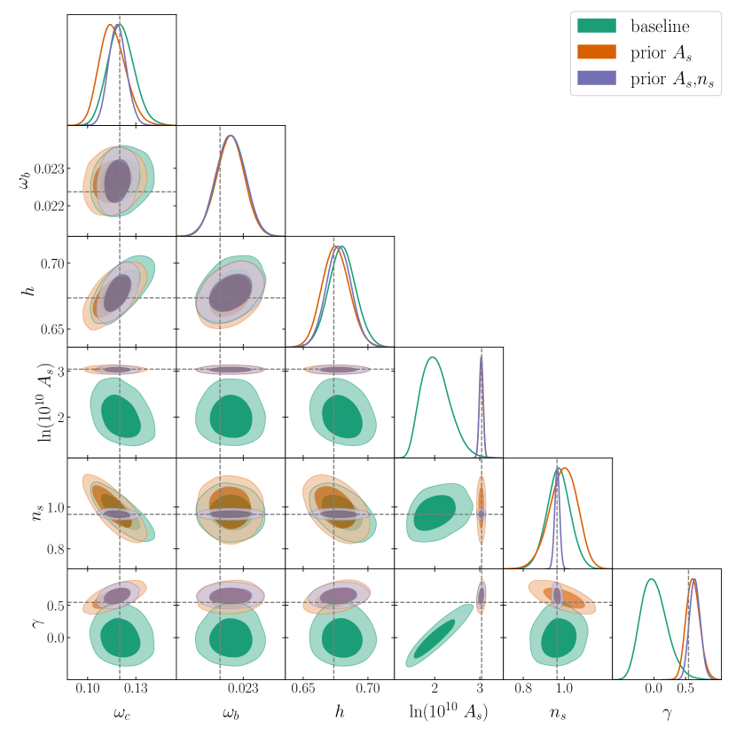
Figure 1: Marginalised posterior distribution for the cosmological parameters for the $\gamma$CDM cosmology and the three prior choices, as detailed in the legend. We fit all three multipoles and use $k_{\rm max}=0.2~{}h~{}{\rm Mpc}^{-1}$. Grey dashed lines mark the Planck best-fit values ($\Lambda$CDM prediction for $\gamma$).

Parameter	baseline	prior on $A_{s}$	prior on $A_{s}$, $n_{s}$
$\omega_{c}$	$0.1208^{+0.0076}_{-0.0086}$	$0.1157^{+0.0072}_{-0.0090}$	$0.1186^{+0.0052}_{-0.0058}$
	(0.1216)	(0.1165)	(0.1196)
$\omega_{b}$	$0.02267\pm 0.00039$	$0.02265\pm 0.00038$	$0.02266\pm 0.00038$
	(0.02298)	(0.02292)	(0.02275)
$h$	$0.680\pm 0.010$	$0.675\pm 0.011$	$0.678\pm 0.010$
	(0.682)	(0.682)	(0.681)
$\ln(10^{10}~{}A_{s})$	$2.030^{+0.248}_{-0.371}$	$3.034\pm 0.042$	$3.033\pm 0.042$
	(2.190)	(3.055)	(3.065)
$n_{s}$	$0.973\pm 0.057$	$0.996^{+0.072}_{-0.062}$	$0.966\pm 0.012$
	(0.970)	(0.994)	(0.970)
$\gamma$	$0.007^{+0.170}_{-0.229}$	$0.617^{+0.098}_{-0.110}$	$0.647\pm 0.085$
	(0.149)	(0.614)	(0.655)
$\sigma_{8}$	$0.498^{+0.047}_{-0.096}$	$0.796\pm 0.030$	$0.801\pm 0.029$
	(0.534)	(0.807)	(0.819)

Table 1: Mean values and 68% c.l. values for $\gamma$CDM with fixed neutrino mass $M_{\nu}=0.06~{}{\rm eV}$ for the three prior choices. We show the best-fit values in parentheses, and include derived constraints on $\sigma_{8}$.

We then open up the parameter space and allow the neutrino mass to vary as a free parameter. It is worth noting that we do not expect to obtain tight constraints on the neutrino mass, as previous analyses already highlighted the inability of BOSS data alone to do so [23, 98, 31]; in fact, as discussed in [23] the precision of BOSS data does not allow to detect the step in the power spectrum which marks the free streaming length of massive neutrinos, restricting detectable signatures only to changes to the overall amplitude. Nevertheless, our goal is to study possible degeneracies between $\gamma$ and $M_{\nu}$, and the impact of massive neutrinos on the constraints on $\gamma$. We modify the theoretical model as described in Sec. 2.3, and explore the same three options for priors as for the $\gamma$CDM case. The marginalised posteriors for $\gamma\nu$CDM are shown in Fig. 2, and the 68% c.l., mean and best-fit values for the cosmological parameters are listed in Table 2.

We first note that the baseline shows a similar shift in the two-dimensional marginalised posteriors for $\gamma$ and $A_{s}$ as the one of Fig. 1. This is again due to the presence of strong degeneracies between the parameters that control the amplitude of the power spectrum. However, the error on $\gamma$ is not affected by the introduction of $M_{\nu}$, and in fact there seems to be no degeneracy between the two. This is actually due to the fact that such degeneracy is mild compared to the others and to the size of the error bars on BOSS data (see e.g. Fig. 12 where we perform forecasts for Stage-IV surveys, an anti-correlation between $\gamma$ and $M_{\nu}$ can clearly be seen).

When we impose Planck priors on the primordial parameters on the other hand we can see a mild degeneracy emerge between $\gamma$ and $M_{\nu}$, which leads to marginally lower values for $\gamma$ with respect to $\gamma$CDM. Concerning neutrinos, as expected the data are not very constraining, and we only provide (somewhat large) upper limits. It is worth commenting on the case with a CMB prior on $A_{s}$, where the model seems to be picking up a large value for $M_{\nu}$: we argue that this is to be ascribed to the model trying to lower the amplitude by exploiting the degeneracy between $M_{\nu}$ and $n_{s}$. More specifically, in the baseline case the amplitude is mostly controlled by $A_{s}$; when that is fixed by the prior, other parameters change to compensate: mostly $\gamma$, but also the neutrino mass, resulting in a looser constraint on $M_{\nu}$ in that case. However, this is only possible if the change in the shape of the power spectrum due to massive neutrinos is compensated by a change in $n_{s}$. When $n_{s}$ is also fixed by the Planck prior, there is less freedom in the shape and thus the constraint on $M_{\nu}$ tightens again.

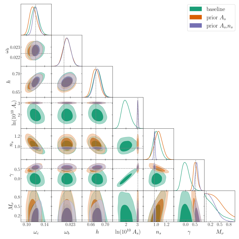
Figure 2: Marginalised posterior distribution for the cosmological parameters for $\gamma\nu$CDM for the three prior choices. We use $k_{\rm max}=0.2~{}h~{}{\rm Mpc}^{-1}$ and a flat prior $M_{\nu}\sim\mathcal{U}(0,1)~{}{\rm eV}$ for the neutrino mass. Grey dashed lines mark the Planck best-fit values (with the $\Lambda$CDM prediction for $\gamma$ and minimal neutrino mass $M_{\nu}=0.06~{}{\rm eV}$).

Parameter	baseline	prior on $A_{s}$	prior on $A_{s}$,$n_{s}$
$\omega_{c}$	$0.1193^{+0.0072}_{-0.0088}$	$0.1146^{+0.0070}_{-0.0090}$	$0.1202^{+0.0054}_{-0.0063}$
	(0.1173)	(0.1184)	(0.1195)
$\omega_{b}$	$0.02266\pm 0.00038$	$0.02265\pm 0.00039$	$0.02267\pm 0.00038$
	(0.02284)	(0.02292)	(0.02264)
$h$	$0.678\pm 0.011$	$0.673\pm 0.011$	$0.6779\pm 0.010$
	(0.675)	(0.683)	(0.681)
$\ln(10^{10}~{}A_{s})$	$2.004^{+0.298}_{-0.412}$	$3.035\pm 0.042$	$3.034\pm 0.042$
	(2.290)	(3.028)	(3.040)
$n_{s}$	$1.009^{+0.061}_{-0.074}$	$1.043\pm 0.079$	$0.967\pm 0.012$
	(0.977)	(1.028)	(0.957)
$\gamma$	$0.001^{+0.165}_{-0.232}$	$0.534^{+0.091}_{-0.12}$	$0.612^{+0.075}_{-0.090}$
	(0.183)	(0.526)	(0.61)
$M_{\nu}$	$<0.372$	$<0.478$	$<0.298$
	(0.038)	(0.362)	(0.016)
$\sigma_{8}$	$0.496^{+0.054}_{-0.108}$	$0.806^{+0.031}_{-0.034}$	$0.809\pm 0.031$
	(0.550)	(0.818)	(0.806)

Table 2: Mean values and 68% c.l. values for $\gamma\nu$CDM for the three prior choices. We show the best-fit values in parentheses, and include derived constraints on $\sigma_{8}$.

In Fig. 3 we plot the one-dimensional marginalised posterior distributions for $\gamma$ for all cases described in this section, to allow for an easier comparison between the constraints we get for this parameter. We mark the best-fit values with dashed lines, following the same color scheme of Fig. 1 and 2, and the $\Lambda$CDM prediction with solid grey lines. As we can see, adopting CMB priors on the primordial parameters shifts the peak of the posterior from (projection affected) negative values to values consistent with the $\Lambda$CDM prediction, albeit slightly larger. Moreover, the difference between the peak of the posterior and the best-fit for the case without CMB-based priors is a hint of the projection which affects the marginalised posteriors.

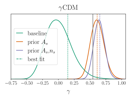
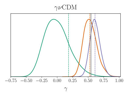
Figure 3: Marginalised one-dimensional posterior distribution for the $\gamma$ parameter for $\gamma$CDM (left) and $\gamma\nu$CDM (right), for the three prior choices as stated in the legend. Dashed vertical lines mark the best-fit values corresponding to the maximum of the marginalised posterior distribution; the solid grey line corresponds to the $\Lambda$CDM prediction.

Our results are broadly consistent with previous analyses of the BOSS data, although an exact comparison is difficult due to different choices in the analysis setup and datasets included. The main novelty of this work is the use of a full-shape approach, as opposed to template fitting adopted in the official BOSS analysis, and the exploration of the impact of priors on the inferred parameters. Moreover, most previous works take advantage of a joint analysis with CMB data, which results in generally tighter constraints. Nevertheless, we report here some of the recent measurements of $\gamma$ that used BOSS galaxies as the main dataset for comparison, highlighting the main differences with respect to this work: [28] found $\gamma=0.566\pm 0.058$ combining BOSS DR12 galaxies with Planck CMB data and SNIa data. Additionally, [27] provides joint constraints on $\gamma$ and the neutrino mass $M_{\nu}$, although they used a previous data release (DR11) and again performed a joint fit with CMB data: they found $\gamma=0.67\pm 0.14$, $M_{\nu}=0.25^{+0.13}_{-0.22}$. A joint analysis with the galaxy bispectrum was performed in [99], finding $\gamma=0.733^{+0.068}_{-0.069}$. All these works are official analyses from the BOSS collaboration, and adopt a fixed template for the power spectrum multipoles. More recently, [100] performed a similar analysis combining data from BOSS, DES and Planck, finding $\gamma=0.633^{+0.025}_{-0.024}$. Also in this case the power spectrum was fitted using a fixed template, as opposed to the full-shape fit we perform in this work.

Overall, our strongest constraints (those where we impose CMB-based priors on the primordial parameters) show a marginal preference for a high value of $\gamma$, consistent for example with [100]. However, in our case the deviation from the $\Lambda$CDM prediction is $\sim 1\sigma$, as opposed to the $\sim 4\sigma$ discrepancy found in that work. In general, our constraints are weaker than those obtained in previous works. This can be attributed to the fact that we only rely on LSS data and include CMB information merely in terms of priors on the primordial parameters: given the degeneracies between the additional parameters of $\gamma$CDM and $\gamma\nu$CDM and the other parameters, some of which are tightly constrained by the CMB, it is no surprise that performing a joint analysis with Planck data can yield tighter constraints. This can also be approximated by including Gaussian priors derived from Planck on all cosmological parameters, see Appendix F of [101] for a comparison.

Another possible way of gaining in constraining power without resorting to CMB information would be to use higher-order statistics such as the galaxy bispectrum. Indeed, the tree-level bispectrum does not depend on $b_{\Gamma_{3}}$, and its inclusion in the analysis can therefore break the degeneracy between $b_{\mathcal{G}_{2}}$ and $b_{\Gamma_{3}}$, leading to improved constraints on the linear bias $b_{1}$ (see [23, 81] for a full-shape joint analysis of BOSS data). While the impact on cosmological parameters is somewhat marginal in the context of $\Lambda$CDM and Stage-III surveys, it can become significant for extended models where there are strong degeneracies between parameters controlling the amplitude: a tighter constraint on $b_{1}$ implies a more precise measurement of $A_{s}$ and therefore of $\gamma$. Some work towards quantifying the impact of including the bispectrum for beyond-$\Lambda$CDM models has already been done in [50] in the context of simulations, where a $\sim 30\%$ improvement was found for a power spectrum and bispectrum joint analysis for an interacting dark energy model. We leave a proper exploration of the impact of the bispectrum in the context of $\gamma$CDM and $\gamma\nu$CDM to a future work.

4.2 Projection effects

In this section we study in more details the prior volume effects found for $\gamma$CDM and $\gamma\nu$CDM when no CMB priors are applied (green contours in Fig. 1 and 2, in particular the $A_{s}$–$\gamma$ plane). The presence of projection effects is already highlighted by the shift between the peak of the one-dimensional marginalised posterior and the best-fit point, see Fig. 3. To better investigate this we adopt two approaches: first we perform a consistency check using synthetic data, then we carry out profiling of the posterior.

For the consistency check we perform the same analysis described in Sec. 4.1 on a synthetic datavector generated with a fiducial cosmology and set of nuisance parameters. We note that the ability of our pipeline to recover the cosmological parameters correctly has been validated with N-body simulations, and we are using the same theoretical model to generate the datavector and fit it, which should lead to perfect agreement between the input and inferred parameters. We use the same covariance computed from the ‘MultiDark-Patchy’ mock catalogues adopted in the BOSS analysis, and include (synthetic) BAO information. As fiducial parameters we adopt the best-fit values of Planck [1], while the nuisance parameters are determined by maximising the BOSS likelihood with cosmology fixed to the Planck values. Our results are plotted in Fig. 4 (purple contours and lines), where we also include the baseline result of Fig. 1 for comparison (green contours and lines).

Figure 4: Posterior distribution for the cosmological parameters for the BOSS data (green) and synthetic data generated with the Planck fiducial cosmology (purple). We fix the total neutrino mass to $M_{\nu}=0.06~{}{\rm eV}$ and use a scale-cut of $k_{\rm max}=0.2~{}h~{}{\rm Mpc}^{-1}$. Grey dashed lines mark the fiducial cosmology used to generate the synthetic data.

The two-dimensional marginalised posteriors for the synthetic data exhibit a very similar behaviour as the one we observed in the BOSS data, with a strong shift in the posterior towards low values of $A_{s}$ and $\gamma$ and almost perfect overlap with the posterior obtained from BOSS data. As discussed above, this effect can be ascribed to the presence of extreme degeneracies in the extended parameter space, which lead to a highly non-Gaussian posterior. As a consequence, the marginalisation process can result in apparent biases in the two-dimensional confidence regions, as discussed thoroughly in [102]. In that work, the author proposes to use profile distributions to assess the impact of marginalisation. As opposed to marginalisation, this profile likelihood (PL) approach allows one to obtain a one-dimensional distribution by evaluating the posterior over a scan of a parameter of interest, $\theta_{i}$, while maximising the posterior with respect to all other parameters $\theta_{k}$, $k\neq i$. This profile distribution is not biased by projection effects, since it is centred on the maximum of the full posterior. For non-Gaussian posteriors, as is the case here, the resulting distribution will be different than the usual marginalised distribution obtained via integration over the marginalised parameters. Depending on the type of non-Gaussianity, this distribution can be broader or narrower over the parameter of interest. This difference between integration and maximisation of the posterior is approximately given by the so-called Laplace term, which accounts for volume effects as explained in Ref. [103].

Ref. [102] suggests performing this profiling step directly on the MCMC samples. However, in addition to resulting in noisy distributions, this is not ideal in our case, since we sample over the analytically marginalised posterior and we therefore expect additional projection due to that pre-marginalisation step. We profile instead the full posterior using the MINOS algorithm implemented in the iminuit package [104]. Our parameter of interest is the growth index $\gamma$, for which we plot the PL in the left panel of Fig. 5, and compare to the one-dimensional marginalised posterior from the MCMC in the right panel. Additionally, we compare the confidence intervals obtained from the MCMC to those obtained from the profiling in Fig. 6.

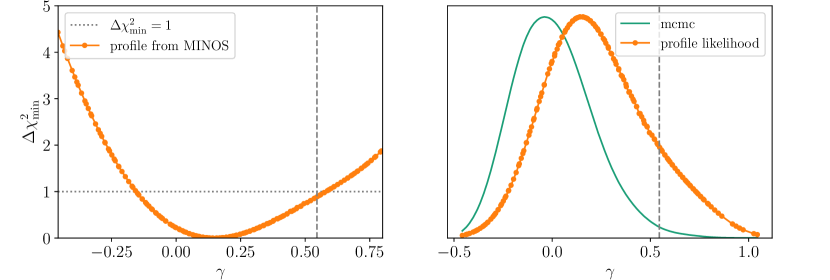
Figure 5: Left: $\Delta\chi^{2}_{\rm min}$ for a set of values for $\gamma$ obtained from profiling the likelihood with MINOS. The horizontal dotted line marks $\Delta\chi^{2}_{\rm min}=1$, which is used to determine confidence intervals. Right: comparison between the marginalised posterior obtained from the mcmc (green curve) and the PL (orange curve and datapoints). The dashed vertical line marks the $\Lambda$CDM prediciton.

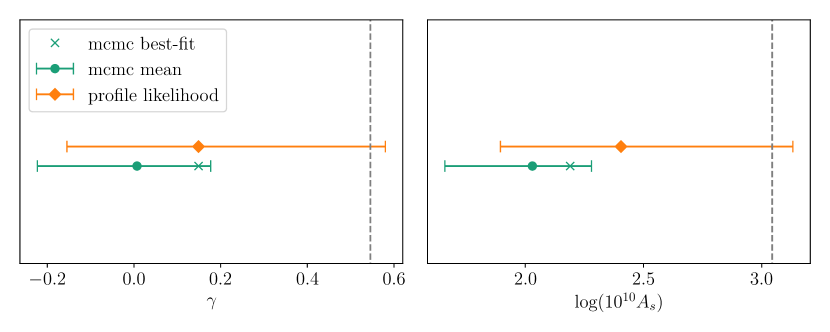
Figure 6: Comparison between the mean values and confidence intervals obtained from the marginalised posterior (green points and error bars) and the PL (orange points and error bars) for $\gamma$ (left) and $\ln(10^{10}~{}A_{s})$ (right). We show the best-fit points obtained from the MCMC with crosses. The dashed vertical line marks the $\Lambda$CDM prediciton.

Fig. 5 shows a clear shift of the PL towards the $\Lambda$CDM prediction with respect to the marginalised posterior. Moreover, the confidence intervals are larger in the case of the PL, making the results consistent with $\Lambda$CDM. We also note how the best-fit points from the MCMC (orange crosses in Fig. 6) are close to the PL results, though still somewhat lower in $A_{s}$. This demonstrates the presence of additional projection effects due to the analytic marginalisation of linear nuisance parameters in the posterior sampled in the MCMC. Overall, the use of the profile likelihood shows a more conservative result, which appears, at least in this case, to reflect better the effect of the large degeneracy between the amplitude parameters on the final one-dimensional constraint on $\gamma$. Note that should the posterior be closer to the Gaussian case, the difference between marginalising and profiling would disappear, so we expect projection effects to disappear with more constraining data.

As mentioned already in Sec 4, the presence of volume (or projection) effects was already highlighted in a number of recent works performing the full-shape analysis of BOSS data in the context of beyond-$\Lambda$CDM models [105, 96, 32, 34]. It is expected that the higher precision of forthcoming data will mitigate this effect, as also suggested by the forecasts we present in Sec. 4.3. However, projections can also be alleviated by the combination with additional probes or the inclusion of higher order correlation functions. In general, we recommend extreme care in the choice of priors, especially when constraining beyond-$\Lambda$CDM models.

4.3 Forecasts for Stage IV surveys

In this section we present forecasts for a Stage-IV spectroscopic galaxy survey, focusing in particular on DESI-like galaxies. Similarly to what described in Sec. 4.2, we generate and fit synthetic datavectors with the same EFTofLSS theoretical model. The aim is twofold: on one hand, we wish to provide forecasted constraints on $\gamma$ and jointly on $\gamma$ and $M_{\nu}$, on the other hand, we can assess the ability of the higher precision measurement of reducing the projection effects. Despite a number of approximations we make in our forecasting strategy, which we highlight below, we expect the results to give a more realistic picture of the outcome of future surveys, as opposed to the standard Fisher matrix approach. The latter, while extremely useful due to its low computational cost, has been shown to be unable to capture complex features in the likelihood, which can arise in the context of strong degeneracies between parameters and highly non-Gaussian posteriors (see e.g. [106, 107, 108, 109]).

We generate three sets of synthetic datavectors, assuming Planck values for the cosmological parameters and simulating the three galaxy samples that are the target of DESI: the bright galaxy sample (BGS), luminous red galaxies (LRGs), and star-forming emission line galaxies (ELG). We follow [10] and compute expected values for the linear bias and number density of the samples, which we list in Table 3 together with the respective effective volume. Specifically, we assume constant values for the combination $b_{1}(z)D(z)$, where $D(z)$ is the linear growth factor evaluated at the central redshift of each bin, and use $b_{\rm LRG}(z)D(z)=1.7$, $b_{\rm ELG}(z)D(z)=0.84$, and $b_{\rm BGS}(z)D(z)=1.34$.

Galaxy sample	$z_{\rm eff}$	$V_{s}~{}[{\rm Gpc}^{3}/h^{3}]$	$b_{1}$	$\bar{n}\,[h^{3}/{\rm Mpc}^{3}]$
BGS	0.2	1.8	1.135	0.013
LRGs	0.8	12	2.56	$3.2\times 10^{-4}$
ELG	1.2	17	1.51	$3.7\times 10^{-4}$

Table 3: Parameters used to generate the synthetic DESI-like datavectors for the forecasts. We follow [10] in computing the effective redshift $z_{\rm eff}$, the volume $V_{s}$ and number density $\bar{n}$, and determine the linear bias $b_{1}$ assuming constant, sample-specific values for the combination $b_{1}(z)D(z)$ as specified in the text.

All redshift bins have size $\Delta z=0.4$ and are centered on the $z_{\rm eff}$ values listed in the table. We compute an analytic covariance matrix, assuming no cross correlation between the redshift bins / samples. Specifically, we use the following [110]:

$$C_{\ell_{1}\ell_{2}}(k_{i},k_{j})=\frac{(2\ell_{1}+1)(2\ell_{2}+1)}{N_{k}}\int_{-1}^{1}{\rm d}\mu~{}\mathcal{L}_{\ell_{1}}(\mu_{i})\mathcal{L}_{\ell_{2}}(\mu_{j})\left[P(\mbox{\boldmath$k$}_{i})+\frac{1}{\bar{n}}\right]\left[P({\mbox{\boldmath$k$}}_{j})+\frac{1}{\bar{n}}\right]\,,$$ (4.1)

where $\mu_{i}$ is the cosine between $\mbox{\boldmath$k$}_{i}$ and the line of sight, $\mathcal{L}_{\ell}$ is the Legendre polynomial of order $\ell$, $\bar{n}$ is the number density and $N_{k}=4\pi k^{2}\Delta k~{}V_{s}/(2\pi)^{3}$ is the number of Fourier modes within a given $k$-bin of size $\Delta k$, $V_{s}$ being the survey volume. For the power spectrum $P(\mbox{\boldmath$k$})$ in Eq. 4.1 we use the Kaiser approximation [111]:

$$P(\mbox{\boldmath$k$})=\left(b_{1}+f\mu^{2}\right)^{2}P_{L}(k)\,.$$ (4.2)

As for priors, we use the same ones we adopted for the baseline BOSS analysis of Sec. 3.2, specifically we impose no prior on the primordial parameters $A_{s}$ and $n_{s}$, both to showcase the constraining power of LSS alone and to assess potential projection effects in the context of Stage-IV surveys. The resulting power spectrum multipoles for the three samples, with corresponding error bars, are shown in Fig. 7.

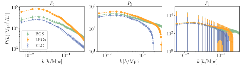
Figure 7: Power spectrum multipoles for the three galaxy samples in our synthetic DESI-like dataset: BGS (green, triangle markers), LRGs (orange, round markers) and ELGs (blue, crosses). The error bars are the square roots of the diagonal elements of the analytic covariance matrix.

We fit the three galaxy samples separately and then combine them, and explore two options for the scale cuts: a pessimistic one with $k_{\rm max}=0.15~{}h~{}{\rm Mpc}^{-1}$ and an optimistic one with $k_{\rm max}=0.25~{}h~{}{\rm Mpc}^{-1}$. Our results for $\gamma$CDM are shown in Fig. 9 (8) for the optimistic (pessimistic) case, and summarised in Table 4. Moreover, we perform the same analysis for $\gamma\nu$CDM and show the results in Fig. 11 (10) for the optimistic (pessimistic) case, while the constraints are listed in Table 5.

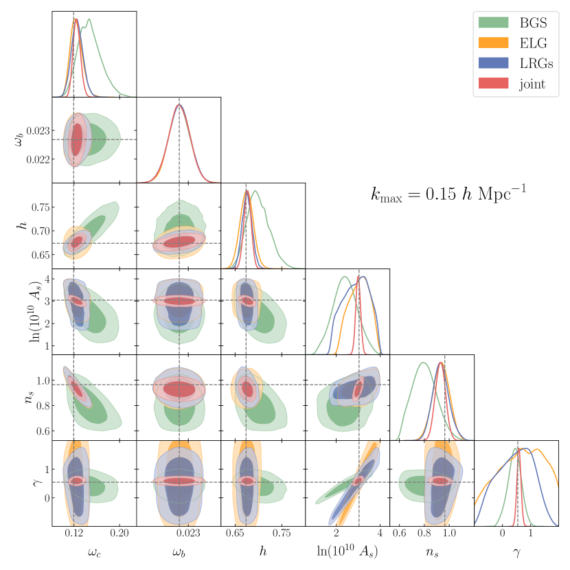
Figure 8: Marginalised posterior for $\gamma$CDM for the pessimistic case with $k_{\rm max}=0.15~{}h~{}{\rm Mpc}^{-1}$. We fit the three samples separately and jointly, as detailed in the legend. Dashed grey lines mark the fiducial values.

Figure 9: Marginalised posterior for $\gamma$CDM for the optimistic case with $k_{\rm max}=0.25~{}h~{}{\rm Mpc}^{-1}$. We fit the three samples separately and jointly, as detailed in the legend. Dashed grey lines mark the fiducial values.

Figure 10: Marginalised posterior for $\gamma\nu$CDM for the pessimistic case with $k_{\rm max}=0.15~{}h~{}{\rm Mpc}^{-1}$. We fit the three samples separately and jointly, as detailed in the legend. Dashed grey lines mark the fiducial values.

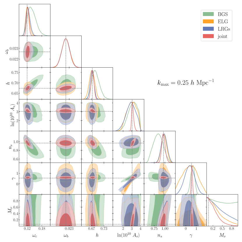
Figure 11: Marginalised posterior for $\gamma\nu$CDM for the optimistic case with $k_{\rm max}=0.25~{}h~{}{\rm Mpc}^{-1}$. We fit the three samples separately and jointly, as detailed in the legend. Dashed grey lines mark the fiducial values.

Parameter	BGS	ELGs	LRGs	joint
Pessimistic $k_{\rm max}=0.15~{}h~{}{\rm Mpc}^{-1}$
$\omega_{c}$	$0.148^{+0.016}_{-0.023}$	$0.1242^{+0.0088}_{-0.012}$	$0.1256^{+0.0095}_{-0.011}$	$0.1250^{+0.0059}_{-0.0069}$
	(0.1352)	(0.1202)	(0.1228)	(0.1212)
$\omega_{b}$	$0.02268\pm 0.00038$	$0.02269\pm 0.00037$	$0.02268\pm 0.00038$	$0.02268\pm 0.00038$
	(0.02255)	(0.02230)	(0.02306)	(0.02303)
$h$	$0.700^{+0.020}_{-0.027}$	$0.675\pm 0.014$	$0.676\pm 0.011$	$0.6765\pm 0.0078$
	(0.688)	(0.671)	(0.679)	(0.676)
$\ln(10^{10}~{}A_{s})$	$2.41\pm 0.55$	$3.06^{+0.56}_{-0.43}$	$2.90^{+0.71}_{-0.55}$	$3.00\pm 0.11$
	(2.27)	(3.26)	(3.27)	(3.04)
$n_{s}$	$0.801^{+0.090}_{-0.11}$	$0.935\pm 0.066$	$0.933^{+0.060}_{-0.069}$	$0.930\pm 0.041$
	(0.752)	(0.955)	(0.950)	(0.950)
$\gamma$	$0.43^{+0.25}_{-0.22}$	$0.64^{+1.1}_{-0.63}$	$0.45^{+0.76}_{-0.58}$	$0.587\pm 0.072$
	(0.37)	(0.94)	(0.81)	(0.57)
$\sigma_{8}$	$0.65^{+0.11}_{-0.19}$	$0.84^{+0.15}_{-0.25}$	$0.80^{+0.15}_{-0.31}$	$0.804\pm 0.037$
	(0.55)	(0.903)	(0.912)	(0.809)
Optimistic $k_{\rm max}=0.25~{}h~{}{\rm Mpc}^{-1}$
$\omega_{c}$	$0.137^{+0.014}_{-0.019}$	$0.1216^{+0.0068}_{-0.0088}$	$0.1231^{+0.0076}_{-0.0098}$	$0.1221^{+0.0048}_{-0.0055}$
	(0.1298)	(0.1175)	(0.1176)	(0.1135)
$\omega_{b}$	$0.02269\pm 0.00038$	$0.02268\pm 0.00038$	$0.02268\pm 0.00037$	$0.02267\pm 0.00038$
	(0.02205)	(0.02245)	(0.02196)	(0.02139)
$h$	$0.688^{+0.016}_{-0.021}$	$0.676\pm 0.013$	$0.6752\pm 0.0087$	$0.6755\pm 0.0067$
	(0.679)	(0.676)	(0.669)	(0.662)
$\ln(10^{10}~{}A_{s})$	$3.04^{+0.57}_{-0.42}$	$3.01^{+0.46}_{-0.51}$	$2.96\pm 0.48$	$3.063\pm 0.074$
	(2.81)	(2.91)	(3.51)	(3.10)
$n_{s}$	$0.80\pm 0.10$	$0.949\pm 0.052$	$0.947\pm 0.056$	$0.947\pm 0.034$
	(0.872)	(0.975)	(0.965)	(0.982)
$\gamma$	$0.68^{+0.22}_{-0.19}$	$0.47\pm 0.75$	$0.47^{+0.57}_{-0.50}$	$0.584\pm 0.058$
	(0.521)	(0.287)	(1.016)	(0.549)
$\sigma_{8}$	$0.85^{+0.17}_{-0.21}$	$0.82^{+0.12}_{-0.25}$	$0.81^{+0.15}_{-0.23}$	$0.822\pm 0.026$
	(0.737)	(0.754)	(1.015)	(0.816)

Table 4: Mean values and 68% c.l. values for $\gamma$CDM with fixed neutrino mass $M_{\nu}=0.06~{}{\rm eV}$ for the three DESI-like galaxy samples fitted separately and jointly. We show the best-fit values in parentheses, and include derived constaints for $\sigma_{8}$.

Parameter	BGS	ELG	LRGs	joint
Pessimistic $k_{\rm max}=0.15~{}h~{}{\rm Mpc}^{-1}$
$\omega_{c}$	$0.149^{+0.016}_{-0.024}$	$0.1243^{+0.0086}_{-0.012}$	$0.1257^{+0.0091}_{-0.011}$	$0.1242^{+0.0060}_{-0.0069}$
	(0.1431 )	(0.1171 )	(0.1181)	(0.1212)
$\omega_{b}$	$0.02269\pm 0.00038$	$0.02269\pm 0.00038$	$0.02268\pm 0.00037$	$0.02268\pm 0.00038$
	(0.02322 )	(0.02274)	(0.02261)	(0.02273)
$h$	$0.701^{+0.020}_{-0.027}$	$0.670\pm 0.015$	$0.672\pm 0.011$	$0.6745\pm 0.0081$
	(0.698 )	(0.676 )	(0.675)	(0.68)
$\ln(10^{10}~{}A_{s})$	$2.47\pm 0.61$	$3.02^{+0.79}_{-0.41}$	$2.85^{+0.96}_{-0.46}$	$3.08^{+0.12}_{-0.19}$
	(1.25 )	(3.32)	(3.25)	(2.99)
$n_{s}$	$0.84\pm 0.11$	$0.967\pm 0.075$	$0.971^{+0.068}_{-0.079}$	$0.958^{+0.043}_{-0.058}$
	(0.816 )	(0.969)	(0.979)	(0.95)
$\gamma$	$0.43\pm 0.23$	$0.51\pm 0.71$	$0.36^{+0.66}_{-0.55}$	$0.590\pm 0.072$
	(-0.07)	(0.04)	(0.81)	(0.563)
$M_{\nu}$	—	$<0.434$	$<0.494$	$<0.314$
	(0.017 )	(0.024)	(0.026)	(0.032)
$\sigma_{8}$	$0.63^{+0.11}_{-0.22}$	$0.79^{+0.22}_{-0.25}$	$0.74^{+0.19}_{-0.30}$	$0.801^{+0.037}_{-0.046}$
	(0.351 )	(0.925)	(0.900)	(0.798 )
Optimistic $k_{\rm max}=0.25~{}h~{}{\rm Mpc}^{-1}$
$\omega_{c}$	$0.1398^{+0.0137}_{-0.0198}$	$0.1216^{+0.0065}_{-0.0087}$	$0.1237^{+0.0072}_{-0.0095}$	$0.1219^{+0.0046}_{-0.0054}$
	(0.1308)	(0.1197)	(0.1208)	(0.1203 )
$\omega_{b}$	$0.02268\pm 0.00038$	$0.02269\pm 0.00038$	$0.02268\pm 0.00037$	$0.02267\pm 0.00037$
	(0.02265)	(0.02278)	(0.02325)	(0.02207)
$h$	$0.690^{+0.016}_{-0.021}$	$0.672\pm 0.013$	$0.673\pm 0.009$	$0.675\pm 0.007$
	(0.684)	(0.678)	(0.683)	(0.671)
$\ln(10^{10}~{}A_{s})$	$3.106^{+0.666}_{-0.393}$	$2.989^{+0.644}_{-0.496}$	$2.893^{+0.615}_{-0.516}$	$3.116^{+0.084}_{-0.145}$
	(2.87)	(3.12)	(3.26)	(3.07)
$n_{s}$	$0.844\pm 0.110$	$0.978^{+0.058}_{-0.065}$	$0.983\pm 0.067$	$0.968^{+0.035}_{-0.045}$
	(0.877)	(0.958)	(0.979)	(0.962)
$\gamma$	$0.655^{+0.202}_{-0.180}$	$0.405\pm 0.668$	$0.366\pm 0.462$	$0.588\pm 0.058$
	(0.539)	(0.748)	(0.795)	(0.598)
$M_{\nu}$	—	$<0.368$	$<0.489$	$<0.270$
	(0.214)	(0.039)	(0.052)	(0.082)
$\sigma_{8}$	$0.817^{+0.181}_{-0.205}$	$0.776^{+0.174}_{-0.250}$	$0.738^{+0.166}_{-0.239}$	$0.815^{+0.026}_{-0.031}$
	(0.732)	(0.841)	(0.910)	(0.822)

Table 5: Mean values and 68% c.l. values for $\gamma\nu$CDM for the three DESI-like galaxy samples fitted separately and jointly. We show the best-fit values in parentheses, and include derived constraints for $\sigma_{8}$.

For the joint analysis in $\gamma$CDM we find $\sigma(\gamma)=0.058~{}(0.072)$ for the optimistic (pessimistic) case, which represents an improvement of $\sim 85\%$ with respect to the BOSS results when no CMB priors are imposed. For $\gamma\nu$CDM we find the same values, despite the introduction of $M_{\nu}$ as a free parameter. As for massive neutrinos, we get $M_{\nu}<0.27~{}(<0.314)$ at 68% c.l. for the optimistic (pessimistic) case, with a very modest improvement with respect to the constraints obtained from BOSS data. Such a dramatic improvement in the constraints on $\gamma$ is due to the combination of the different samples: each sample features a slightly different orientation of the degeneracy between $A_{s}$ and $\gamma$, which is then broken when we perform the joint fit.

Focusing on the projection effects which heavily affected the BOSS analysis, we can clearly see how they are strongly mitigated by the increased precision of the mock data and the combination of multiple samples at different redshifts. In fact, for the joint analysis of the three galaxy samples the deviation between the input and best-fit values for $\gamma$ is $\sim 0.1\sigma$, with the exception of the $\gamma\nu$CDM cosmology in the optimistic case where the deviation is $\sim 0.4\sigma$. On the other hand, some projection is still present in the fits for the single samples, although we can always recover the input value at the 1$\sigma$ level. It is also worth noting how the inclusion of more nonlinear modes can further alleviate the projection. For example, from the BGS sample we obtain $\gamma=0.43^{+0.25}_{-0.22}~{}(0.37)$ in the pessimistic case and $\gamma=0.68^{+0.22}_{-0.19}~{}(0.521)$ in the optimistic case, with the shift between the best-fit point and the input value reduced from $0.37\sigma$ to $0.06\sigma$.

A proper comparison to other forecasts in the literature is complicated, because the results depend strongly on the forecasting strategy. Nonetheless, we try to summarise previous results and highlight the differences with this work. Overall we find weaker constraints on $\gamma$, which can mainly be attributed to the following reasons:

• most works rely on the Fisher matrix formalism, known to be unable to properly describe the likelihood in presence of strong degeneracies in the parameter space;

• most works use a linear model for the power spectrum, with a significantly smaller number of nuisance parameters;

• most works perform a joint analysis with CMB information, which, as discussed above, can tightly constrain some of the parameters which are most degenerate with $\gamma$.

Forecasts for the $\gamma$ parameterisation for Stage-IV surveys can be found in [112]. The authors use a Fisher matrix approach and a linear model for the power spectrum, limiting their analysis at $k_{\rm max}<0.1~{}h~{}{\rm Mpc}^{-1}$, and find an overly optimistic $\sigma(\gamma)=0.0096$ for the case with fixed neutrino mass and dark energy parameter. This result is mainly driven by the differences in the dimensionality of the parameter space considered: their modelling only involves six parameters (nine when they also consider massive neutrinos and evolving dark energy), with only one (linear) bias, and no parameter controlling the overall amplitude of the power spectrum, whose inclusion can undermine the ability to measure $\gamma$.

A more comprehensive collection of forecasts for future experiments can be found in [113], that however still relies on a Fisher matrix approach. All forecasts presented there include Planck CMB and are limited to a linear model for the power spectrum, and can therefore be expected to be more constraining than our analysis. Nonetheless, the authors find $\sigma(\gamma)=0.025$, which is closer to our forecasted $\sigma(\gamma)=0.058$ than the results of [112].

We note that lifting some of the simplifications we make when generating the synthetic dataset could improve our constraints. For example, considering several redshift bins per sample can yield more precise measurements of the cosmological parameters, including $\gamma$ [114, 115], but it also leads to an increased number of nuisance parameters and increased shot-noise per redshift bin. Moreover, some of the effects we are not accounting for are expected to result in reduced constraining power, for example the assumption of a Gaussian covariance, neglecting the convolution with the survey window function and in general additional observational systematics which can increase the size of the error bars on the measurements [116, 117].

We finally comment on our forecasts on massive neutrinos. A measurement of the neutrino mass is one of the main goals of Stage-IV surveys, with predicted errors well below the detection threshold (e.g. [113, 118, 101]). In this sense, our forecasts might seem too pessimistic, given our best case scenario gives $M_{\nu}<0.27~{}{\rm eV}$ at 68% c.l. Once again, most previous forecasts take advantage of a combined analysis with CMB data from Planck, able to put tight constraints on the primordial parameters $A_{s}$ and $n_{s}$. The latter are degenerate with the neutrino mass $M_{\nu}$, as can be seen in Fig. 11 (or equivalently and more clearly in the green contours of Fig. 12): we therefore expect a joint analysis to be extremely beneficial. We do not perform such an analysis here, but we can get a sense of the impact by imposing a 3$\sigma$ Planck prior on the primordial parameters, as done in Sec. 4.1 for the BOSS analysis. We only focus on the combination of the three redshift bins for the optimistic case with $k_{\rm max}=0.25h~{}{\rm Mpc}^{-1}$. Our results are shown in Fig. 12 and Table 6. As expected, the CMB prior on $A_{s}$ and $n_{s}$ breaks the degeneracies and brings the upper limit on the neutrino mass down to $M_{\nu}<0.175~{}{\rm eV}$ at 68% c.l., with a 35% improvement over the case with no priors.

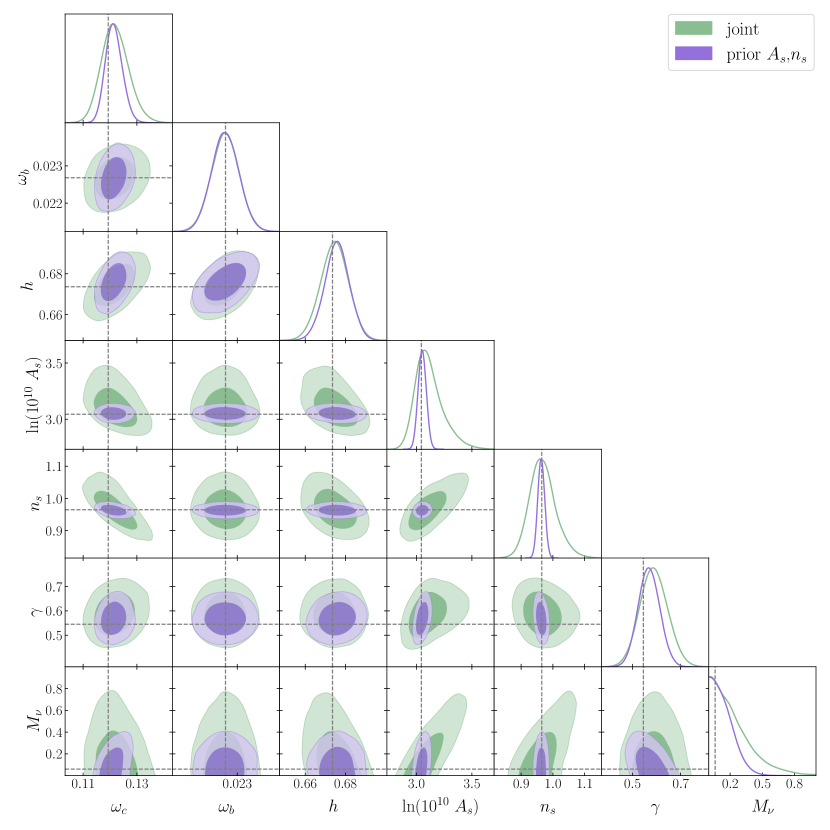
Figure 12: Comparison between the forecast when no CMB prior is imposed (green lines and contours) and the case with 3$\sigma$ Planck priors on $A_{s}$ and $n_{s}$ (purple lines and contours). We use $k_{\rm max}=0.25~{}h~{}{\rm Mpc}^{-1}$.

Parameter	baseline	prior on $A_{s}$,$n_{s}$
$\omega_{c}$	$0.1219^{+0.0046}_{-0.0054}$	$0.1215^{+0.0028}_{-0.0034}$
	(0.1203 )	(0.1211)
$\omega_{b}$	$0.02267\pm 0.00037$	$0.02268\pm 0.00037$
	(0.02207)	(0.02266)
$h$	$0.6746\pm 0.0069$	$0.6758\pm 0.0062$
	(0.6712)	(0.6767)
$\ln(10^{10}~{}A_{s})$	$3.116^{+0.084}_{-0.14}$	$3.052\pm 0.037$
	(3.074 )	(3.016 )
$n_{s}$	$0.968^{+0.035}_{-0.045}$	$0.963\pm 0.011$
	(0.962)	(0.957)
$\gamma$	$0.588\pm 0.058$	$0.568\pm 0.045$
	(0.598)	(0.554)
$M_{\nu}$	$<0.270$	$<0.175$
	(0.082)	(0.033)
$\sigma_{8}$	$0.815^{+0.026}_{-0.031}$	$0.804\pm 0.020$
	(0.822)	(0.807)

Table 6: Best-fit and 68% c.l. values for the DESI forecasts with 3$\sigma$ Planck priors on $A_{s}$,$n_{s}$. We use $k_{\rm max}=0.25~{}h~{}{\rm Mpc}^{-1}$.

Despite being quite large in the context of a detection of the neutrino mass, our results are generally compatible with [69]; there, the authors performed a validation against N-body simulations of a similar 1-loop model for the power spectrum as the one adopted here. For a $25~{}{\rm Gpc}^{3}/h^{3}$ survey, similar in volume to our combined DESI-like mocks, they found $M_{\nu}<0.49~{}{\rm eV}$ at 68% c.l. and conclude that 2-point summary statistics from spectroscopic clustering alone might not be sufficient detect the neutrino mass. Beside the combination with CMB data, we expect the combination with higher order statistics such as the bispectrum to bring significant improvements [119, 120]. We leave the study of the impact of the bispectrum on the determination of the neutrino mass scale to a future work. Further improvement should come from using photometric probes, namely cosmic shear and galaxy-galaxy lensing [41].

5 Conclusions

We presented the full-shape analysis of the power spectrum multipoles measured from BOSS DR12 galaxies with the inclusion of post-reconstruction BAO data. We used the windowless measurements of [81] combined with BAO measurements obtained from a variety of data-sets [81, 84, 85, 86]. We provided constraints on a single parameter extension of $\Lambda$CDM which allows for deviations from the standard scenario in the growth functions, the so-called ‘growth index’ (or $\gamma$) parameterisation. We also explored the case with the total neutrino mass as a free parameter, and provided joint constraints for $\gamma$ and $M_{\nu}$. Our theoretical model for the power spectrum is based on the EFTofLSS and takes advantage of the bacco emulator for the linear power spectrum and the FAST-PT algorithm for a fast evaluation of the likelihood.

We explored different options for the priors on the parameters that determine the primordial power spectrum, $A_{s}$ and $n_{s}$, finding that strong degeneracies in the extended parameter space result in large projection effects, especially concerning the parameters which regulate the amplitude of the power spectrum. For this reason, we applied a 3$\sigma$ Planck prior on $A_{s}$ and on both $A_{s}$ and $n_{s}$, and obtained $\gamma=0.647\pm 0.085$ and $\gamma=0.612^{+0.075}_{-0.090}$, respectively, $\sim 1\sigma$ consistent with the $\Lambda$CDM prediction $\gamma=0.55$. For neutrinos we found $M_{\nu}<0.478~{}{\rm eV}$ (Planck prior on $A_{s}$) and $M_{\nu}<0.298~{}{\rm eV}$ (Planck prior on $A_{s}$, $n_{s}$), consistent with previous EFTofLSS-based studies of the BOSS dataset that did not perform a full joint analysis with CMB data [23, 98].

To assess the presence of projection effects in the case when no priors are imposed on the primordial parameters we generated synthetic datavectors with a fiducial set of cosmological and nuisance parameters, and then fitted them using the same numerical covariance used for the BOSS analysis. We found a similar shift of the posterior in the $A_{s}$–$\gamma$ plane as the one found in our baseline BOSS analysis. Additionally, we performed a profile likelihood analysis, finding the maximum of the PL to be closer to the $\Lambda$CDM prediction than the peak of the marginalised posterior, and the confidence intervals derived from the PL to be larger and consistent with $\gamma=0.55$ at 68% c.l..

Overall, we find the EFTofLSS model complemented with Planck priors to provide constraints on $\gamma$ that are only $\sim 30\%$ larger than the official BOSS analysis [28], despite the fact that we did not perform a full joint analysis with CMB data. Additionally, our theoretical model features a significantly larger number of parameters, which is expected to degrade the constraints to some extent. On the other hand, the full-shape approach allows to provide direct constraints on the cosmological parameters.

In the second part of this work we presented forecasts for a Stage-IV spectroscopic survey, focusing on a DESI-like galaxy sample. We generated three synthetic datavectors at three redshifts using different values for the nuisance parameters, to match the expected BGS, LRGs and ELGs samples that are the target of DESI. We computed Gaussian covariance matrices neglecting the cross-correlation between samples, and adopted two different scale-cuts: $k_{\rm max}=0.15~{}h~{}{\rm Mpc}^{-1}$ (pessimistic) and $k_{\rm max}=0.25~{}h~{}{\rm Mpc}^{-1}$ (optimistic). We performed separate fits for each sample and then combined them in a joint analysis, finding the combination to provide significantly tighter constraints, yielding $\sigma(\gamma)=0.058~{}(0.072)$ in the optimistic (pessimistic) case, with a $\sim 85\%$ improvement with respect to our baseline BOSS analysis without CMB-based priors. Concerning neutrinos, we found that the improvement with respect to Stage-III constraints is only marginal, $M_{\nu}<0.27~{}{\rm eV}$ ($M_{\nu}<0.314~{}{\rm eV}$) in the optimistic (pessimistic) case at 68% c.l..

In order to reduce the error bars on $\gamma$ and $M_{\nu}$, but also to keep the projection effects under control, we advocate the combination with additional observables. For example, a joint analysis with Planck data (or the inclusion of CMB-based priors, at least on the primordial parameters), can have a significant impact on the constraints. We explored this by performing a fit of the synthetic DESI-like data where we adopted 3$\sigma$ Planck priors on $A_{s}$ and $n_{s}$. We obtained a $\sim 20\%$ improvement in the measurement of $\gamma$, and $\sim 35\%$ for $M_{\nu}$ with respect to the case with no priors. Similarly, a combination with weak lensing can alleviate the degeneracies and yield tighter constraints [41]. However, an optimal exploitation of galaxy clustering data alone can already go in this direction: as shown in [50], the ability of the bispectrum to better determine the bias parameters can prove crucial in the context of extended models. We leave the study of the impact of the bispectrum for $\gamma$CDM and $\gamma\nu$CDM to a future work.

Appendix A Full contourplots

We show here the two-dimensional marginalised posteriors for the full parameter space sampled in the BOSS analysis presented in Sec. 4.1. The results for $\gamma$CDM are shown in Fig. 13, corresponding to the constraints on cosmological parameters shown in Fig. 1, while $\gamma\nu$CDM results are plotted in Fig. 14, corresponding to the constraints on cosmolofical parameters shown in Fig. 2. The additional model parameters not shown are the ones we analytically marginalise over, namely $b_{\Gamma_{3}}$, the EFT counterterm parameters and the noise parameters. We follow the same color scheme as the main text for the three prior choices, and mark Planck best-fit values with dashed grey lines.

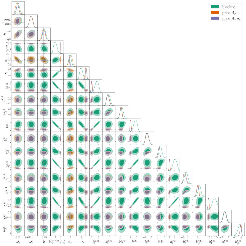
Figure 13: Two-dimensional marginalised posterior for all parameters for the BOSS analysis for $\gamma$CDM and $k_{\rm max}=0.2~{}h~{}{\rm Mpc}^{-1}$ (see Fig. 1). We use the same color scheme as the main text to show the three prior choices. Dashed grey lines mark the Planck best-fit values ($\Lambda$CDM prediction for $\gamma$).

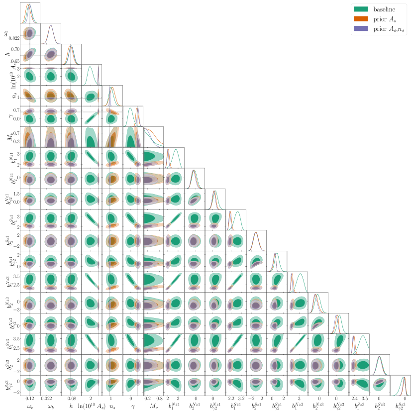
Figure 14: Two-dimensional marginalised posterior for all parameters for the BOSS analysis with $\gamma\nu$CDM and $k_{\rm max}=0.2~{}h~{}{\rm Mpc}^{-1}$ (see Fig. 2). We use the same color scheme as the main text to show the three prior choices. Dashed grey lines mark the Planck best-fit values (with the $\Lambda$CDM prediction for $\gamma$ and minimal neutrino mass $M_{\nu}=0.06~{}{\rm eV}$).

Appendix B Massive neutrinos with fixed $\gamma$

We perform a complementary analysis of the BOSS data with free neutrino mass but with the $\gamma$ parameter fixed to its $\Lambda$CDM value, $\gamma=0.55$. The two-dimensional marginalised posteriors are shown in Fig. 15, and the best-fits are summarised in Table 7. We impose a wide, flat prior on the neutrino mass $\mathcal{U}(0,1)~{}{\rm eV}$, covering the parameter space allowed by the emulator for the linear power spectrum. We explore again the three options for the priors on the primordial parameters, and obtain the following constraints for the total neutrino mass: $M_{\nu}<0.319$, best-fit 0.137 (baseline), $M_{\nu}=0.34^{+0.13}_{-0.28}$, best-fit 0.141 (prior on $A_{s}$), $M_{\nu}=0.29^{+0.12}_{-0.24}$, best-fit 0.111 (prior on $A_{s}$ and $n_{s}$), where values are expressed in eV. Additionally, for the baseline analysis we find a higher value of the amplitude: $\log(10^{10}~{}A_{s})=2.90^{+0.17}_{-0.21}$, as opposed to $\log(10^{10}~{}A_{s})=2.67\pm 0.17$ found in the $\Lambda$CDM analysis of [32] (that used the same pipeline and priors adopted here).

Comparing to previous constraints on the total neutrino mass from the full-shape analysis of BOSS data, we find our results to be in excellent agreement with [98]. There, the authors perform a similar EFT-based analysis of $\Lambda$CDM + massive neutrinos, also finding that having the neutrino mass as a free parameter allows for a slightly larger value of $A_{s}$, closer to the Planck best-fit value, which is then balanced by a peak in the posterior at $M_{\nu}=0.29^{+0.31}_{-0.18}~{}{\rm eV}$. The same EFTofLSS model adopted in this work was also used in [121] to constrain the total neutrino mass from BOSS data. However, in that work the fit is performed jointly with CMB data from Planck, which results in significantly tighter constraints: $M_{\nu}<0.16~{}{\rm eV}$ at 95% c.l..

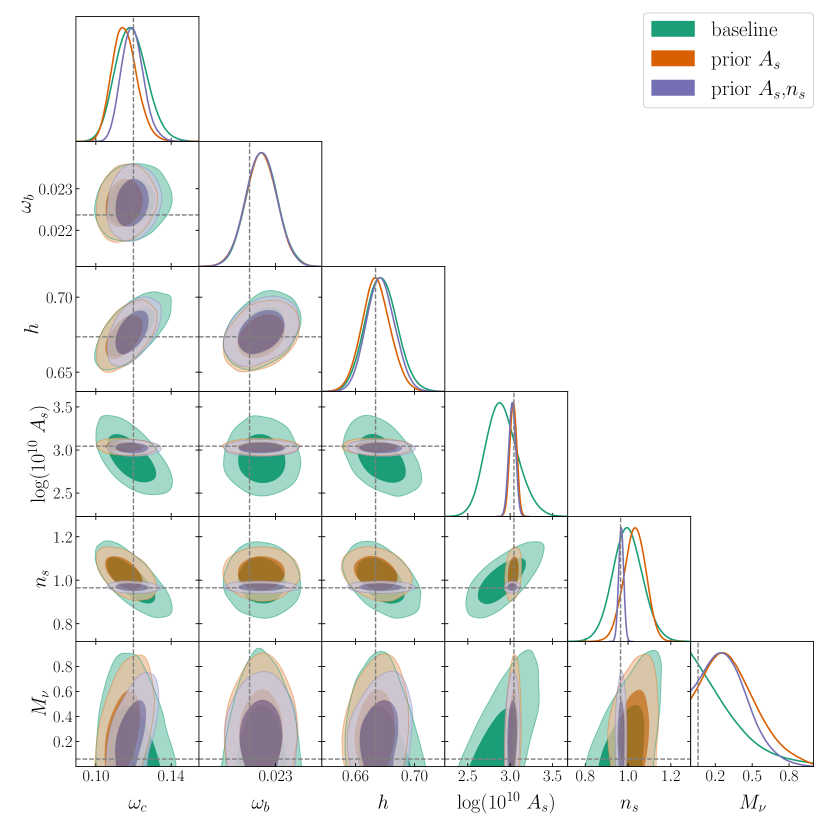
Figure 15: Marginalised posterior distribution for the cosmological parameters for $\Lambda$CDM with massive neutrinos and the three prior choices, as detailed in the legend. We fit all three multipoles and use $k_{\rm max}=0.2~{}h~{}{\rm Mpc}^{-1}$. Grey dashed lines mark the Planck best-fit values.

Parameter	baseline	prior on $A_{s}$	prior on $A_{s}$, $n_{s}$
$\omega_{c}$	$0.1189^{+0.0076}_{-0.0090}$	$0.1153^{+0.0058}_{-0.0072}$	$0.1195^{+0.0053}_{-0.0063}$
	(0.1147)	(0.1099)	(0.1132)
$\omega_{b}$	$0.02267\pm 0.00038$	$0.02265\pm 0.00038$	$0.02266\pm 0.00038$
	(0.02237)	(0.02241)	(0.02260)
$h$	$0.677\pm 0.011$	$0.6739\pm 0.0097$	$0.6770\pm 0.0096$
	(0.675)	(0.676)	(0.676)
$\log(10^{10}~{}A_{s})$	$2.90^{+0.17}_{-0.21}$	$3.037\pm 0.041$	$3.024\pm 0.040$
	(3.00)	(3.07)	(3.04)
$n_{s}$	$0.998\pm 0.071$	$1.032^{+0.054}_{-0.048}$	$0.968\pm 0.012$
	(0.997)	(1.048 )	(0.9691)
$M_{\nu}$	$<0.319$	$0.34^{+0.13}_{-0.28}$	$0.29^{+0.12}_{-0.24}$
	(0.137)	(0.141)	(0.111)
$\sigma_{8}$	$0.763^{+0.049}_{-0.081}$	$0.807^{+0.029}_{-0.033}$	$0.802^{+0.027}_{-0.032}$
	(0.783)	(0.802)	(0.779)

Table 7: Best-fit and 68% c.l. values for the analysis with free neutrino mass and $\gamma=0.55$ for the three prior choices. We also derive best-fit values for $\sigma_{8}$.

References

- [1] Planck Collaboration, N. Aghanim, Y. Akrami, M. Ashdown, J. Aumont, C. Baccigalupi et al., Planck 2018 results. VI. Cosmological parameters, A&A 641 (2020) A6 [1807.06209].
- [2] S. Alam, M. Aubert, S. Avila, C. Balland, J.E. Bautista, M.A. Bershady et al., Completed SDSS-IV extended Baryon Oscillation Spectroscopic Survey: Cosmological implications from two decades of spectroscopic surveys at the Apache Point Observatory, Phys. Rev. D 103 (2021) 083533 [2007.08991].
- [3] C. Heymans, T. Tröster, M. Asgari, C. Blake, H. Hildebrandt, B. Joachimi et al., KiDS-1000 Cosmology: Multi-probe weak gravitational lensing and spectroscopic galaxy clustering constraints, A&A 646 (2021) A140 [2007.15632].
- [4] T.M.C. Abbott, M. Aguena, A. Alarcon, S. Allam, O. Alves, A. Amon et al., Dark Energy Survey Year 3 results: Cosmological constraints from galaxy clustering and weak lensing, Phys. Rev. D 105 (2022) 023520 [2105.13549].
- [5] A.G. Riess, A.V. Filippenko, P. Challis, A. Clocchiatti, A. Diercks, P.M. Garnavich et al., Observational Evidence from Supernovae for an Accelerating Universe and a Cosmological Constant, AJ 116 (1998) 1009 [astro-ph/9805201].
- [6] S. Perlmutter, G. Aldering, G. Goldhaber, R.A. Knop, P. Nugent, P.G. Castro et al., Measurements of and from 42 High-Redshift Supernovae, ApJ 517 (1999) 565 [astro-ph/9812133].
- [7] L. Verde, T. Treu and A.G. Riess, Tensions between the early and late Universe, Nature Astronomy 3 (2019) 891 [1907.10625].
- [8] E. Di Valentino, O. Mena, S. Pan, L. Visinelli, W. Yang, A. Melchiorri et al., In the realm of the Hubble tension-a review of solutions, Classical and Quantum Gravity 38 (2021) 153001 [2103.01183].
- [9] L. Perivolaropoulos and F. Skara, Challenges for CDM: An update, New A Rev. 95 (2022) 101659 [2105.05208].
- [10] DESI Collaboration, A. Aghamousa, J. Aguilar, S. Ahlen, S. Alam, L.E. Allen et al., The DESI Experiment Part I: Science,Targeting, and Survey Design, arXiv e-prints (2016) arXiv:1611.00036 [1611.00036].
- [11] R. Laureijs, J. Amiaux, S. Arduini, J.L. Auguères, J. Brinchmann, R. Cole et al., Euclid Definition Study Report, arXiv e-prints (2011) arXiv:1110.3193 [1110.3193].
- [12] The LSST Dark Energy Science Collaboration, R. Mandelbaum, T. Eifler, R. Hložek, T. Collett, E. Gawiser et al., The LSST Dark Energy Science Collaboration (DESC) Science Requirements Document, arXiv e-prints (2018) arXiv:1809.01669 [1809.01669].
- [13] D. Spergel, N. Gehrels, C. Baltay, D. Bennett, J. Breckinridge, M. Donahue et al., Wide-Field InfrarRed Survey Telescope-Astrophysics Focused Telescope Assets WFIRST-AFTA 2015 Report, arXiv e-prints (2015) arXiv:1503.03757 [1503.03757].
- [14] L. Amendola, S. Appleby, A. Avgoustidis, D. Bacon, T. Baker, M. Baldi et al., Cosmology and fundamental physics with the Euclid satellite, Living Reviews in Relativity 21 (2018) 2 [1606.00180].
- [15] S. Alam et al., Towards testing the theory of gravity with DESI: summary statistics, model predictions and future simulation requirements, JCAP 11 (2021) 050 [2011.05771].
- [16] F. Bernardeau, S. Colombi, E. Gaztañaga and R. Scoccimarro, Large-scale structure of the Universe and cosmological perturbation theory, Phys. Rep. 367 (2002) 1 [astro-ph/0112551].
- [17] D. Baumann, A. Nicolis, L. Senatore and M. Zaldarriaga, Cosmological non-linearities as an effective fluid, J. Cosmology Astropart. Phys. 2012 (2012) 051 [1004.2488].
- [18] J.J.M. Carrasco, M.P. Hertzberg and L. Senatore, The effective field theory of cosmological large scale structures, Journal of High Energy Physics 2012 (2012) 82 [1206.2926].
- [19] M. Pietroni, G. Mangano, N. Saviano and M. Viel, Coarse-grained cosmological perturbation theory, J. Cosmology Astropart. Phys. 2012 (2012) 019 [1108.5203].
- [20] J.E. McEwen, X. Fang, C.M. Hirata and J.A. Blazek, FAST-PT: a novel algorithm to calculate convolution integrals in cosmological perturbation theory, J. Cosmology Astropart. Phys. 2016 (2016) 015 [1603.04826].
- [21] X. Fang, J.A. Blazek, J.E. McEwen and C.M. Hirata, FAST-PT II: an algorithm to calculate convolution integrals of general tensor quantities in cosmological perturbation theory, J. Cosmology Astropart. Phys. 2017 (2017) 030 [1609.05978].
- [22] M. Simonović, T. Baldauf, M. Zaldarriaga, J.J. Carrasco and J.A. Kollmeier, Cosmological perturbation theory using the FFTLog: formalism and connection to QFT loop integrals, J. Cosmology Astropart. Phys. 2018 (2018) 030 [1708.08130].
- [23] G. d’Amico, J. Gleyzes, N. Kokron, K. Markovic, L. Senatore, P. Zhang et al., The cosmological analysis of the SDSS/BOSS data from the Effective Field Theory of Large-Scale Structure, J. Cosmology Astropart. Phys. 2020 (2020) 005 [1909.05271].
- [24] M.M. Ivanov, M. Simonović and M. Zaldarriaga, Cosmological parameters from the BOSS galaxy power spectrum, J. Cosmology Astropart. Phys. 2020 (2020) 042 [1909.05277].
- [25] S.-F. Chen, Z. Vlah and M. White, A new analysis of galaxy 2-point functions in the BOSS survey, including full-shape information and post-reconstruction BAO, J. Cosmology Astropart. Phys. 2022 (2022) 008 [2110.05530].
- [26] F. Beutler, S. Saito, H.-J. Seo, J. Brinkmann, K.S. Dawson, D.J. Eisenstein et al., The clustering of galaxies in the SDSS-III Baryon Oscillation Spectroscopic Survey: testing gravity with redshift space distortions using the power spectrum multipoles, MNRAS 443 (2014) 1065 [1312.4611].
- [27] F. Beutler, S. Saito, J.R. Brownstein, C.-H. Chuang, A.J. Cuesta, W.J. Percival et al., The clustering of galaxies in the SDSS-III Baryon Oscillation Spectroscopic Survey: signs of neutrino mass in current cosmological data sets, MNRAS 444 (2014) 3501 [1403.4599].
- [28] E.-M. Mueller, W. Percival, E. Linder, S. Alam, G.-B. Zhao, A.G. Sánchez et al., The clustering of galaxies in the completed SDSS-III Baryon Oscillation Spectroscopic Survey: constraining modified gravity, MNRAS 475 (2018) 2122 [1612.00812].
- [29] M.M. Ivanov, E. McDonough, J.C. Hill, M. Simonović, M.W. Toomey, S. Alexander et al., Constraining early dark energy with large-scale structure, Phys. Rev. D 102 (2020) 103502 [2006.11235].
- [30] G. D’Amico, L. Senatore and P. Zhang, Limits on wCDM from the EFTofLSS with the PyBird code, J. Cosmology Astropart. Phys. 2021 (2021) 006 [2003.07956].
- [31] A. Semenaite, A.G. Sánchez, A. Pezzotta, J. Hou, A. Eggemeier, M. Crocce et al., Beyond CDM constraints from the full shape clustering measurements from BOSS and eBOSS, arXiv e-prints (2022) arXiv:2210.07304 [2210.07304].
- [32] P. Carrilho, C. Moretti and A. Pourtsidou, Cosmology with the EFTofLSS and BOSS: dark energy constraints and a note on priors, J. Cosmology Astropart. Phys. 2023 (2023) 028 [2207.14784].
- [33] T. Simon, P. Zhang, V. Poulin and T.L. Smith, Updated constraints from the effective field theory analysis of the BOSS power spectrum on early dark energy, Phys. Rev. D 107 (2023) 063505 [2208.05930].
- [34] L. Piga, M. Marinucci, G. D’Amico, M. Pietroni, F. Vernizzi and B.S. Wright, Constraints on modified gravity from the BOSS galaxy survey, J. Cosmology Astropart. Phys. 2023 (2023) 038 [2211.12523].
- [35] P.J.E. Peebles, The large-scale structure of the universe (1980).
- [36] E.V. Linder, Cosmic growth history and expansion history, Phys. Rev. D 72 (2005) 043529 [astro-ph/0507263].
- [37] G.R. Dvali, G. Gabadadze and M. Porrati, 4-D gravity on a brane in 5-D Minkowski space, Phys. Lett. B 485 (2000) 208 [hep-th/0005016].
- [38] E.V. Linder and R.N. Cahn, Parameterized beyond-Einstein growth, Astroparticle Physics 28 (2007) 481 [astro-ph/0701317].
- [39] Y. Gong, Growth factor parametrization and modified gravity, Phys. Rev. D 78 (2008) 123010 [0808.1316].
- [40] Y. Wen, N.-M. Nguyen and D. Huterer, Sweeping Horndeski Canvas: New Growth-Rate Parameterization for Modified-Gravity Theories, arXiv e-prints (2023) arXiv:2304.07281 [2304.07281].
- [41] Euclid Collaboration, A. Blanchard, S. Camera, C. Carbone, V.F. Cardone, S. Casas et al., Euclid preparation. VII. Forecast validation for Euclid cosmological probes, A&A 642 (2020) A191 [1910.09273].
- [42] J. Lesgourgues and S. Pastor, Massive neutrinos and cosmology, Phys. Rep. 429 (2006) 307 [astro-ph/0603494].
- [43] A. Perko, L. Senatore, E. Jennings and R.H. Wechsler, Biased Tracers in Redshift Space in the EFT of Large-Scale Structure, arXiv e-prints (2016) arXiv:1610.09321 [1610.09321].
- [44] L. Fonseca de la Bella, D. Regan, D. Seery and S. Hotchkiss, The matter power spectrum in redshift space using effective field theory, J. Cosmology Astropart. Phys. 2017 (2017) 039 [1704.05309].
- [45] A. Chudaykin, M.M. Ivanov, O.H.E. Philcox and M. Simonović, Nonlinear perturbation theory extension of the Boltzmann code CLASS, Phys. Rev. D 102 (2020) 063533 [2004.10607].
- [46] A. Oddo, E. Sefusatti, C. Porciani, P. Monaco and A.G. Sánchez, Toward a robust inference method for the galaxy bispectrum: likelihood function and model selection, J. Cosmology Astropart. Phys. 2020 (2020) 056 [1908.01774].
- [47] A. Oddo, F. Rizzo, E. Sefusatti, C. Porciani and P. Monaco, Cosmological parameters from the likelihood analysis of the galaxy power spectrum and bispectrum in real space, J. Cosmology Astropart. Phys. 2021 (2021) 038 [2108.03204].
- [48] F. Rizzo, C. Moretti, K. Pardede, A. Eggemeier, A. Oddo, E. Sefusatti et al., The halo bispectrum multipoles in redshift space, J. Cosmology Astropart. Phys. 2023 (2023) 031 [2204.13628].
- [49] P. Carrilho, C. Moretti, B. Bose, K. Markovič and A. Pourtsidou, Interacting dark energy from redshift-space galaxy clustering, J. Cosmology Astropart. Phys. 2021 (2021) 004 [2106.13163].
- [50] M. Tsedrik, C. Moretti, P. Carrilho, F. Rizzo and A. Pourtsidou, Interacting dark energy from the joint analysis of the power spectrum and bispectrum multipoles with the EFTofLSS, MNRAS 520 (2023) 2611 [2207.13011].
- [51] P. McDonald and A. Roy, Clustering of dark matter tracers: generalizing bias for the coming era of precision LSS, J. Cosmology Astropart. Phys. 2009 (2009) 020 [0902.0991].
- [52] V. Assassi, D. Baumann, D. Green and M. Zaldarriaga, Renormalized halo bias, J. Cosmology Astropart. Phys. 2014 (2014) 056 [1402.5916].
- [53] V. Desjacques, D. Jeong and F. Schmidt, Large-scale galaxy bias, Phys. Rep. 733 (2018) 1 [1611.09787].
- [54] M.M. Abidi and T. Baldauf, Cubic halo bias in Eulerian and Lagrangian space, J. Cosmology Astropart. Phys. 2018 (2018) 029 [1802.07622].
- [55] E. Castorina, E. Sefusatti, R.K. Sheth, F. Villaescusa-Navarro and M. Viel, Cosmology with massive neutrinos II: on the universality of the halo mass function and bias, J. Cosmology Astropart. Phys. 2014 (2014) 049 [1311.1212].
- [56] E. Castorina, C. Carbone, J. Bel, E. Sefusatti and K. Dolag, DEMNUni: the clustering of large-scale structures in the presence of massive neutrinos, J. Cosmology Astropart. Phys. 2015 (2015) 043 [1505.07148].
- [57] R. Scoccimarro, H.M.P. Couchman and J.A. Frieman, The Bispectrum as a Signature of Gravitational Instability in Redshift Space, ApJ 517 (1999) 531 [astro-ph/9808305].
- [58] Y. Donath and L. Senatore, Biased tracers in redshift space in the EFTofLSS with exact time dependence, J. Cosmology Astropart. Phys. 2020 (2020) 039 [2005.04805].
- [59] M. Crocce and R. Scoccimarro, Nonlinear evolution of baryon acoustic oscillations, Phys. Rev. D 77 (2008) 023533 [0704.2783].
- [60] L. Senatore and M. Zaldarriaga, The IR-resummed Effective Field Theory of Large Scale Structures, J. Cosmology Astropart. Phys. 2015 (2015) 013 [1404.5954].
- [61] Z. Vlah, U. Seljak, M. Yat Chu and Y. Feng, Perturbation theory, effective field theory, and oscillations in the power spectrum, J. Cosmology Astropart. Phys. 2016 (2016) 057 [1509.02120].
- [62] D.J. Eisenstein and W. Hu, Baryonic Features in the Matter Transfer Function, ApJ 496 (1998) 605 [astro-ph/9709112].
- [63] C. Alcock and B. Paczynski, An evolution free test for non-zero cosmological constant, Nature 281 (1979) 358.
- [64] A. Lewis, A. Challinor and A. Lasenby, Efficient computation of CMB anisotropies in closed FRW models, ApJ 538 (2000) 473 [astro-ph/9911177].
- [65] G. Aricò, R.E. Angulo and M. Zennaro, Accelerating Large-Scale-Structure data analyses by emulating Boltzmann solvers and Lagrangian Perturbation Theory, arXiv e-prints (2021) arXiv:2104.14568 [2104.14568].
- [66] A. Spurio Mancini, D. Piras, J. Alsing, B. Joachimi and M.P. Hobson, CosmoPower: emulating cosmological power spectra for accelerated Bayesian inference from next-generation surveys, Mon. Not. Roy. Astron. Soc. 511 (2022) 1771 [2106.03846].
- [67] R. Calderon, D. Felbacq, R. Gannouji, D. Polarski and A.A. Starobinsky, Global properties of the growth index of matter inhomogeneities in the Universe, Phys. Rev. D 100 (2019) 083503 [1908.00117].
- [68] R. Calderon, D. Felbacq, R. Gannouji, D. Polarski and A.A. Starobinsky, Global properties of the growth index: Mathematical aspects and physical relevance, Phys. Rev. D 101 (2020) 103501 [1912.06958].
- [69] H.E. Noriega, A. Aviles, S. Fromenteau and M. Vargas-Magaña, Fast computation of non-linear power spectrum in cosmologies with massive neutrinos, J. Cosmology Astropart. Phys. 2022 (2022) 038 [2208.02791].
- [70] D. Baumann, D. Green and B. Wallisch, Searching for light relics with large-scale structure, J. Cosmology Astropart. Phys. 2018 (2018) 029 [1712.08067].
- [71] B. Giblin, M. Cataneo, B. Moews and C. Heymans, On the road to per cent accuracy - II. Calibration of the non-linear matter power spectrum for arbitrary cosmologies, MNRAS 490 (2019) 4826 [1906.02742].
- [72] A. Boyle and F. Schmidt, Neutrino mass constraints beyond linear order: cosmology dependence and systematic biases, J. Cosmology Astropart. Phys. 2021 (2021) 022 [2011.10594].
- [73] S. Saito, M. Takada and A. Taruya, Nonlinear power spectrum in the presence of massive neutrinos: Perturbation theory approach, galaxy bias, and parameter forecasts, Phys. Rev. D 80 (2009) 083528 [0907.2922].
- [74] M. Levi and Z. Vlah, Massive neutrinos in nonlinear large scale structure: A consistent perturbation theory, arXiv e-prints (2016) arXiv:1605.09417 [1605.09417].
- [75] L. Senatore and M. Zaldarriaga, The Effective Field Theory of Large-Scale Structure in the presence of Massive Neutrinos, arXiv e-prints (2017) arXiv:1707.04698 [1707.04698].
- [76] A. Aviles and A. Banerjee, A Lagrangian perturbation theory in the presence of massive neutrinos, J. Cosmology Astropart. Phys. 2020 (2020) 034 [2007.06508].
- [77] A. Aviles, A. Banerjee, G. Niz and Z. Slepian, Clustering in massive neutrino cosmologies via Eulerian Perturbation Theory, J. Cosmology Astropart. Phys. 2021 (2021) 028 [2106.13771].
- [78] S. Alam et al., The Eleventh and Twelfth Data Releases of the Sloan Digital Sky Survey: Final Data from SDSS-III, The Astrophysical Journal Supplement Series 219 (2015) 12 [1501.00963].
- [79] H. Gil-Marín, W.J. Percival, J.R. Brownstein, C.-H. Chuang, J.N. Grieb, S. Ho et al., The clustering of galaxies in the SDSS-III Baryon Oscillation Spectroscopic Survey: RSD measurement from the LOS-dependent power spectrum of DR12 BOSS galaxies, MNRAS 460 (2016) 4188 [1509.06386].
- [80] F. Beutler, H.-J. Seo, S. Saito, C.-H. Chuang, A.J. Cuesta, D.J. Eisenstein et al., The clustering of galaxies in the completed SDSS-III Baryon Oscillation Spectroscopic Survey: anisotropic galaxy clustering in Fourier space, MNRAS 466 (2017) 2242 [1607.03150].
- [81] O.H.E. Philcox and M.M. Ivanov, BOSS DR12 full-shape cosmology: CDM constraints from the large-scale galaxy power spectrum and bispectrum monopole, Phys. Rev. D 105 (2022) 043517 [2112.04515].
- [82] O.H.E. Philcox, Cosmology without window functions: Quadratic estimators for the galaxy power spectrum, Phys. Rev. D 103 (2021) 103504 [2012.09389].
- [83] O.H.E. Philcox, Cosmology without window functions. II. Cubic estimators for the galaxy bispectrum, Phys. Rev. D 104 (2021) 123529 [2107.06287].
- [84] F. Beutler, C. Blake, M. Colless, D.H. Jones, L. Staveley-Smith, L. Campbell et al., The 6dF Galaxy Survey: baryon acoustic oscillations and the local Hubble constant, MNRAS 416 (2011) 3017 [1106.3366].
- [85] A.J. Ross, L. Samushia, C. Howlett, W.J. Percival, A. Burden and M. Manera, The clustering of the SDSS DR7 main Galaxy sample - I. A 4 per cent distance measure at z = 0.15, MNRAS 449 (2015) 835 [1409.3242].
- [86] H. du Mas des Bourboux, J. Rich, A. Font-Ribera, V. de Sainte Agathe, J. Farr, T. Etourneau et al., The Completed SDSS-IV Extended Baryon Oscillation Spectroscopic Survey: Baryon Acoustic Oscillations with Ly Forests, ApJ 901 (2020) 153 [2007.08995].
- [87] F.-S. Kitaura, S. Rodríguez-Torres, C.-H. Chuang, C. Zhao, F. Prada, H. Gil-Marín et al., The clustering of galaxies in the SDSS-III Baryon Oscillation Spectroscopic Survey: mock galaxy catalogues for the BOSS Final Data Release, MNRAS 456 (2016) 4156 [1509.06400].
- [88] S.A. Rodríguez-Torres, C.-H. Chuang, F. Prada, H. Guo, A. Klypin, P. Behroozi et al., The clustering of galaxies in the SDSS-III Baryon Oscillation Spectroscopic Survey: modelling the clustering and halo occupation distribution of BOSS CMASS galaxies in the Final Data Release, MNRAS 460 (2016) 1173 [1509.06404].
- [89] D. Foreman-Mackey, D.W. Hogg, D. Lang and J. Goodman, emcee: The MCMC Hammer, PASP 125 (2013) 306 [1202.3665].
- [90] J. Goodman and J. Weare, Ensemble samplers with affine invariance, Communications in Applied Mathematics and Computational Science 5 (2010) 65.
- [91] M. Karamanis, F. Beutler, J.A. Peacock, D. Nabergoj and U. Seljak, Accelerating astronomical and cosmological inference with preconditioned Monte Carlo, MNRAS 516 (2022) 1644 [2207.05652].
- [92] M. Karamanis, D. Nabergoj, F. Beutler, J. Peacock and U. Seljak, pocoMC: A Python package for accelerated Bayesian inference in astronomy and cosmology, The Journal of Open Source Software 7 (2022) 4634 [2207.05660].
- [93] E. Aver, K.A. Olive and E.D. Skillman, The effects of He I 10830 on helium abundance determinations, J. Cosmology Astropart. Phys. 2015 (2015) 011 [1503.08146].
- [94] R.J. Cooke, M. Pettini and C.C. Steidel, One Percent Determination of the Primordial Deuterium Abundance, ApJ 855 (2018) 102 [1710.11129].
- [95] N. Schöneberg, J. Lesgourgues and D.C. Hooper, The BAO+BBN take on the Hubble tension, J. Cosmology Astropart. Phys. 2019 (2019) 029 [1907.11594].
- [96] T. Simon, P. Zhang, V. Poulin and T.L. Smith, On the consistency of effective field theory analyses of BOSS power spectrum, arXiv e-prints (2022) arXiv:2208.05929 [2208.05929].
- [97] G. D’Amico, Y. Donath, M. Lewandowski, L. Senatore and P. Zhang, The BOSS bispectrum analysis at one loop from the Effective Field Theory of Large-Scale Structure, 2206.08327.
- [98] T. Colas, G. d’Amico, L. Senatore, P. Zhang and F. Beutler, Efficient cosmological analysis of the SDSS/BOSS data from the Effective Field Theory of Large-Scale Structure, J. Cosmology Astropart. Phys. 2020 (2020) 001 [1909.07951].
- [99] H. Gil-Marín, W.J. Percival, L. Verde, J.R. Brownstein, C.-H. Chuang, F.-S. Kitaura et al., The clustering of galaxies in the SDSS-III Baryon Oscillation Spectroscopic Survey: RSD measurement from the power spectrum and bispectrum of the DR12 BOSS galaxies, MNRAS 465 (2017) 1757 [1606.00439].
- [100] N.-M. Nguyen, D. Huterer and Y. Wen, Evidence for suppression of structure growth in the concordance cosmological model, arXiv e-prints (2023) arXiv:2302.01331 [2302.01331].
- [101] A. Chudaykin and M.M. Ivanov, Measuring neutrino masses with large-scale structure: Euclid forecast with controlled theoretical error, J. Cosmology Astropart. Phys. 2019 (2019) 034 [1907.06666].
- [102] A. Gómez-Valent, Fast test to assess the impact of marginalization in Monte Carlo analyses and its application to cosmology, Phys. Rev. D 106 (2022) 063506 [2203.16285].
- [103] B. Hadzhiyska, K. Wolz, S. Azzoni, D. Alonso, C. García-García, J. Ruiz-Zapatero et al., Cosmology with 6 parameters in the Stage-IV era: efficient marginalisation over nuisance parameters, 2301.11895.
- [104] F. James and M. Roos, Minuit: A System for Function Minimization and Analysis of the Parameter Errors and Correlations, Comput. Phys. Commun. 10 (1975) 343.
- [105] L. Herold, E.G.M. Ferreira and E. Komatsu, New Constraint on Early Dark Energy from Planck and BOSS Data Using the Profile Likelihood, ApJ 929 (2022) L16 [2112.12140].
- [106] B. Joachimi and A.N. Taylor, Forecasts of non-Gaussian parameter spaces using Box-Cox transformations, MNRAS 416 (2011) 1010 [1103.3370].
- [107] L. Wolz, M. Kilbinger, J. Weller and T. Giannantonio, On the validity of cosmological Fisher matrix forecasts, J. Cosmology Astropart. Phys. 2012 (2012) 009 [1205.3984].
- [108] N. Bellomo, J.L. Bernal, G. Scelfo, A. Raccanelli and L. Verde, Beware of commonly used approximations. Part I. Errors in forecasts, J. Cosmology Astropart. Phys. 2020 (2020) 016 [2005.10384].
- [109] J.L. Bernal, N. Bellomo, A. Raccanelli and L. Verde, Beware of commonly used approximations. Part II. Estimating systematic biases in the best-fit parameters, J. Cosmology Astropart. Phys. 2020 (2020) 017 [2005.09666].
- [110] A. Taruya, T. Nishimichi and S. Saito, Baryon acoustic oscillations in 2D: Modeling redshift-space power spectrum from perturbation theory, Phys. Rev. D 82 (2010) 063522 [1006.0699].
- [111] N. Kaiser, Clustering in real space and in redshift space, MNRAS 227 (1987) 1.
- [112] A. Stril, R.N. Cahn and E.V. Linder, Testing standard cosmology with large-scale structure, MNRAS 404 (2010) 239 [0910.1833].
- [113] A. Font-Ribera, P. McDonald, N. Mostek, B.A. Reid, H.-J. Seo and A. Slosar, DESI and other Dark Energy experiments in the era of neutrino mass measurements, J. Cosmology Astropart. Phys. 2014 (2014) 023 [1308.4164].
- [114] J. Fonseca, J.-A. Viljoen and R. Maartens, Constraints on the growth rate using the observed galaxy power spectrum, J. Cosmology Astropart. Phys. 2019 (2019) 028 [1907.02975].
- [115] J.-A. Viljoen, J. Fonseca and R. Maartens, Constraining the growth rate by combining multiple future surveys, J. Cosmology Astropart. Phys. 2020 (2020) 054 [2007.04656].
- [116] D. Wadekar and R. Scoccimarro, Galaxy power spectrum multipoles covariance in perturbation theory, Phys. Rev. D 102 (2020) 123517 [1910.02914].
- [117] D. Wadekar, M.M. Ivanov and R. Scoccimarro, Cosmological constraints from BOSS with analytic covariance matrices, Phys. Rev. D 102 (2020) 123521 [2009.00622].
- [118] B. Audren, J. Lesgourgues, S. Bird, M.G. Haehnelt and M. Viel, Neutrino masses and cosmological parameters from a Euclid-like survey: Markov Chain Monte Carlo forecasts including theoretical errors, J. Cosmology Astropart. Phys. 2013 (2013) 026 [1210.2194].
- [119] C. Hahn, F. Villaescusa-Navarro, E. Castorina and R. Scoccimarro, Constraining Mν with the bispectrum. Part I. Breaking parameter degeneracies, J. Cosmology Astropart. Phys. 2020 (2020) 040 [1909.11107].
- [120] C. Hahn and F. Villaescusa-Navarro, Constraining Mν with the bispectrum. Part II. The information content of the galaxy bispectrum monopole, J. Cosmology Astropart. Phys. 2021 (2021) 029 [2012.02200].
- [121] M.M. Ivanov, M. Simonović and M. Zaldarriaga, Cosmological parameters and neutrino masses from the final P l a n c k and full-shape BOSS data, Phys. Rev. D 101 (2020) 083504 [1912.08208].
- [122] C.R. Harris, K.J. Millman, S.J. van der Walt, R. Gommers, P. Virtanen, D. Cournapeau et al., Array programming with NumPy, Nature 585 (2020) 357.
- [123] P. Virtanen, R. Gommers, T.E. Oliphant, M. Haberland, T. Reddy, D. Cournapeau et al., SciPy 1.0: Fundamental Algorithms for Scientific Computing in Python, Nature Methods 17 (2020) 261.
- [124] J.D. Hunter, Matplotlib: A 2D Graphics Environment, Computing in Science and Engineering 9 (2007) 90.
- [125] A. Lewis, GetDist: a Python package for analysing Monte Carlo samples, arXiv e-prints (2019) arXiv:1910.13970 [1910.13970].