A9 Intersection Dataset:
All You Need for Urban 3D Camera-LiDAR Roadside Perception

Abstract

Intelligent Transportation Systems (ITS) allow a drastic expansion of the visibility range and decrease occlusions for autonomous driving. To obtain accurate detections, detailed labeled sensor data for training is required. Unfortunately, high-quality 3D labels of LiDAR point clouds from the infrastructure perspective of an intersection are still rare. Therefore, we provide the A9 Intersection Dataset, which consists of labeled LiDAR point clouds and synchronized camera images. Here, we recorded the sensor output from two roadside cameras and LiDARs mounted on intersection gantry bridges. The point clouds were labeled in 3D by experienced annotators. Furthermore, we provide calibration data between all sensors, which allow the projection of the 3D labels into the camera images and an accurate data fusion. Our dataset consists of 4.8k images and point clouds with more than 57.4k manually labeled 3D boxes. With ten object classes, it has a high diversity of road users in complex driving maneuvers, such as left and right turns, overtaking, and U-turns. In experiments, we provided multiple baselines for the perception tasks. Overall, our dataset is a valuable contribution to the scientific community to perform complex 3D camera-LiDAR roadside perception tasks. Find data, code, and more information at https://a9-dataset.com.

TABLE I: Comparison of popular autonomous driving datasets. Here we compare the perspective, the number of frames, the number of classes, the number of labeled objects, the number of tracks, and the license terms. The datasets cover different view perspectives: the vehicle view (V), from the steep elevated view (SE), and from the roadside view (R).

Name	Year	Perspective	# Point Clouds	# Images	# Classes	# 3D Labels	# Tracks	License
KITTI [1]	2013	V	15.4k	15k	8	80k	-	CC BY-NC-SA 3.0
Cityscapes [2]	2016	V	-	25k	30	-	-	Non-Commercial Use
highD [3]	2018	SE	-	1.4M	2	-	20k	Custom
nuScenes[4]	2020	V	400k	1.4M	23	1.4M	-	CC BY-NC-SA 4.0
Waymo [5]	2020	V	200	1M	4	12.6M	7.6M	Custom
inD [6]	2020	SE	-	0.9M	5	-	11.5k	Custom
rounD [7]	2020	SE	-	0.5M	8	-	13.7k	Custom
exiD [8]	2022	SE	-	1.4M	3	-	69k	Custom
MONA [9]	2022	SE	-	11.7M	2	-	702k	Custom
DAIR-V2X∗ [10]	2022	V,R	71k	71k	10	1.2M	-	Non-Commercial Use
IPS300+∗∗ [11]	2022	R	14.1k	14.1k	7	4.5M	-	CC BY-NC-SA 4.0
Rope3D [12]	2022	R	-	50k	13	1.5M	-	Non-Commercial Use
LUMPI [13]	2022	R	90k	200k	6	-	-	CC BY-NC 3.0
A9	2022	R	5.3k	5.4k	10	71.9k	506	CC BY-NC-ND 4.0
- A9 [14]	2022	R	0.5k	0.6k	9	14.5k	-	CC BY-NC-ND 4.0
- A9-I (Ours)	2023	R	4.8k	4.8k	10	57.4k	506	CC BY-NC-ND 4.0
∗ 40% of data from roadside perspective, 60% from vehicle perspective.
∗∗Trucks and buses are sparsely represented which can lead to a limited perception performance.

I INTRODUCTION

The roadside deployment of high-tech sensors to detect road traffic participants offers significant added value for intelligent and autonomous driving. This technology allows the vehicle to react to events and situations that are not covered by the vehicle’s internal sensor range. Thus, the advantage is the drastic expansion of the field of view and the reduction of occlusions. For this reason, we can observe a continuous increase in Intelligent Transportation Systems (ITS) world-wide. It is noticeable that cameras and increasingly LiDARS are used to create a live digital twin of road traffic [15]. To obtain accurate detections with such sensor systems, labeled sensor data is required for training.

Numerous datasets in the field of intelligent and autonomous driving have already been created. Datasets like [1, 4, 2, 5] are taken from the vehicle perspective. In contrast, [3, 16, 7, 8, 9] are recorded from a very steep elevated view from a drone or a high building, so they are more suitable for trajectory prediction and tracking tasks. They are less suitable for 3D object detection because vehicles are far away and are only observed from above. Recently, a few datasets [10, 11, 12, 13, 14] have been acquired from an roadside perspective and are thus suitable for improving perception algorithms for ITS. However, some datasets have deficiencies in their labeling quality, which harm the training of the algorithms (e.g., censored image areas with filled rectangles), or they lack certain vehicle classes (e.g., missing trucks and buses), or the datasets are too small in terms of 3D box labels and attributes.

According to the work mentioned, it can be recognized that high-quality 3D box labels of LiDAR point clouds from the roadside perspective with a wide diversity of traffic participants and scenarios are still rare. Therefore, our A9 Intersection (A9-I) Dataset provides LiDAR point clouds and camera images from a road intersection. The $4.8\text{k}$ labeled point cloud frames, which were labeled by experts, contain complex driving maneuvers such as left and right turns, overtaking maneuvers, and U-turns. With its ten object classes, our dataset has a high variety of road users, including vulnerable road users. Furthermore, we provide synchronized camera images and the extrinsic calibration data between LiDARs and the cameras. These matrices allow the projection of the 3D box labels to the camera images. All in all, our A9-I offers synchronized $4.8\text{k}$ images and $4.8\text{k}$ point clouds with $57.4\text{k}$ 3D box labels with track IDs that were manually labeled. In this work, we show additional comprehensive statistics and the effectiveness of our dataset. Over and beyond, we would like to emphasize that A9-I is an extension of our previous debut the A9 Dataset [14], which covers highway traffic scenarios. Thus, we extend the existing A9 Dataset with additional traffic scenarios on a crowdy intersection and scale it up from $15\text{k}$ labeled 3D box labels to $57.4\text{k}$ including vulnerable road users. In evaluation experiments, we provide multiple baselines for the 3D perception task of 3D object detection with a monocular camera, a LiDAR sensor, and a multi-modal camera-LiDAR setup. Last but not least, we offer our dataset in OpenLABEL format under the Creative Commons License CC BY-NC-ND 4.0 so that it can be widely used by the scientific research community.

In summary, our contributions are:

• A detailed and diverse dataset of $4.8\text{k}$ camera images as well as $4.8\text{k}$ labeled LiDAR point cloud frames. Thereby, we used two synchronized cameras and LiDARS, which cover an intersection from an elevated view of an ITS.

• Extrinsic calibration data between cameras and LiDARs allow an early and late fusion of objects.

• We provide an extensive A9-Devkit to load, transform, split, evaluate and visualize the data.

• $57.4\text{k}$ high-quality manually labeled 3D boxes with $273\text{k}$ attributes for both LiDARS resulting in $38\text{k}$ 3D box labels after data fusion.

• Comprehensive statistics and analysis of the labels, number of points, occlusions, and tracks on the dataset, and the distribution of ten different object classes of road traffic.

• Multiple baselines for the 3D perception task of 3D object detection with a monocular camera, a LiDAR sensor, and a multi-modal camera-LiDAR setup.

II RELATED WORK

As part of the development in the field of autonomous driving and intelligent vehicles, the number of datasets is increasing rapidly. The most popular datasets in this field are KITTI [1], nuScenes [4], Cityscapes [2], and Waymo Open dataset [5]. Except for the Cityscapes, the datasets provide labeled camera images and LiDAR point clouds. These datasets are used to train perception algorithms. Unfortunately, these valuable datasets only contain data from a vehicle’s perspective. Therefore, this ego perspective is suboptimal for transfer learning. Networks trained on a dataset from the vehicle’s perspective do not perform well on data obtained, e.g. from a roadside perspective.

Another sensor perspective is, for example, the elevated view. With this, the scene can ideally be viewed without occlusions. To achieve a high level of perception for this elevated view, training with appropriate datasets is necessary. The focus of the drone dataset family highD [3], inD [16], rounD [7], and exiD [8] is the trajectory of road users in the city as well as in the freeway area. The datasets were recorded by a drone and provide a vast top-down view of the scene. The main limitation is the limited recording time in challenging weather conditions. To overcome this drone-related issue, the MONA [9] dataset provides data that was created with a camera mounted on a building. On the one hand, these datasets are ideal for trajectory research, because they were recorded from a very steep angle to the road. On the other hand, they are less suitable for 3D object detection, because of the missing 3D dimensions.

A dataset, which contains data from an elevated view of an ITS with an angle that is not too steep, is the DAIR-V2X [10]. The main focus of DAIR-V2X is the support of of 3D object detection tasks. It consists of $71\text{k}$ labeled camera images and LiDAR point clouds, $40\%$ of which are from an roadside infrastructure. For this purpose, the dataset covers city roads, highways, and intersections in different weather and lighting conditions. Unfortunately, no exact statistics for this variation or exact sensor specifications are available. As a last point, the quality of the data is further compromised by filled rectangles over privacy-sensitive image areas (e.g., license plates), which can lead to problems during training for object detection. Another dataset from the roadside infrastructure perspective with a camera and LiDAR combination is the IPS300+ [11]. The dataset includes $14\text{k}$ data frames, with an average of $319$ labels per frame. They used $1$ LiDAR and $2$ cameras as a stereo setup with a lens focal length of $4.57~{}\text{mm}$. The dataset was recorded several times a day at one intersection and provides seven different object categories: car, cyclist, pedestrian, tricycle, bus, truck, and engineer car. According to the statistics, unfortunately, there is less representation in the classes of trucks and buses, so that the recognition of these classes will probably be poor. The Roadside Perception 3D dataset (Rope3D) [12] provides $50\text{k}$ images including 3D box labels from an monocular infrastructure camera at an intersection. The missing 3D information of the detected objects in the 2D camera image was added with a LiDAR, which was mounted on a vehicle. In total, the images contain over $1.5\text{M}$ labeled 3D boxes, $670\text{k}$ 2D bounding boxes, in various scenes at different times (daytime, night, dawn/dusk), different weather conditions (sunny, cloudy, rainy), and different traffic densities. Furthermore, the objects are divided into $13$ classes with several attributes. Another roadside infrastructure dataset is LUMPI [13], which was recorded at an intersection in Hanover, Germany. For this purpose, a total of $200\text{k}$ images as well as $90\text{k}$ point clouds were acquired. Three different cameras and five different LiDARs provide several field of views on the scene. Here, different sensor configurations were used for the recordings. The sensor perspective is from a vehicle as well as from the roadside infrastructure. Unfortunately, the number of labels and other detailed information about the labeled objects was not provided. A further contribution in the field of roadside infrastructure data for training perception algorithm is the A9-Dataset [14]. It is our preliminary work and includes $642$ camera images and $456$ LiDAR point clouds. In total, this dataset consists of 1k 3D box labels. The charm is that most camera images contain the same traffic scene from four different viewpoints. Here, we labeled 14k 3D boxes. Moreover, the frames contain $13.17$ 3D box labels in average. For this purpose, we supported the common classes of car, trailer, truck, van, pedestrian, bicycle, bus, and motorcycle in the domain of a highway. The main limitations in our previous work were firstly the small number of labeled LiDAR point clouds and secondly that we only had a simple highway scenario. For this reason, we present an extension to our dataset that addresses these weaknesses.

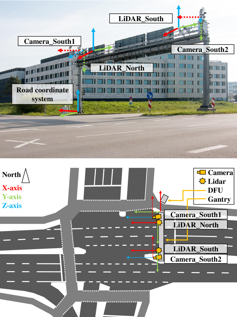
Figure 1: Two cameras and two LiDARs are used to create the A9 Intersection Dataset. The sensors are mounted on a sign gantry and thus record the central intersection area. Then, the Data Fusion Unit (DFU) process the data streams, which results in a fused digital twin of the road traffic. Furthermore, the coordinate systems of the individual sensors and the road coordinate system, which was defined at the northern stem of the bridge, can be taken from the figure.

III A9 INTERSECTION DATASET

In this section, we present the A9 Intersection Dataset. It is an extension of our previous work, the A9-Dataset [14], which covers the highway domain. We describe the sensor setup at our intersection, the data selection and annotation process, and the data structure used. Last, this section contains comprehensive statistics and an introduction to our A9-Devkit.

III-A Sensor Setup

The A9-I Dataset is recorded on the ITS testbed, which was established as part of the Providentia++ project [17, 18]. Here, roadside sensors are set up on a gantry located at the intersection of Schleißheimer Straße (B471) and Zeppelinstraße in Garching near Munich, Germany. For this dataset, we use two cameras and two LiDARs with the following specifications:

• Camera: Basler ace acA1920-50gc, $1920\times 1200$, Sony IMX174, glo. shutter, color, GigE with 8 mm lenses.

• LiDAR: Ouster OS1-64 (gen. 2), 64 vert. layers, $360\text{\textdegree FOV}$, below horizon configuration, $120~{}\text{m}$ range, $1.5-10~{}\text{cm}$ accuracy.

The sensors are mounted side by side on the gantry, as shown in Figure 1. Here, the sensors detect the traffic in the center of the intersection from a height of $7~{}\text{m}$. It is worth mentioning that the cameras and LiDARs are spatiotemporally calibrated. For the temporal calibration, we synchronized the sensors with a Network Time Protocol (NTP) time server, for the extrinsic calibration between the cameras and the LiDARs, we used a targetless extrinsic calibration method, which was inspired by [19].

III-B Data Selection and Annotation

We select the data based on interesting and challenging traffic scenarios like left, right, and U-turns, overtaking maneuvers, tail-gate events, and lane merge scenarios. Furthermore, we take highly diverse and dense traffic situations into account, so that we get an average of over $15$ road users per frame. To cover diverse weather and light conditions in our A9-I Dataset, it consists of $25\%$ nighttime data including heavy rain, and $75\%$ daytime data with sunny and cloudy weather conditions. This enables a good performance of the detector even in challenging weather conditions.

We record camera data at $25\text{ Hz}$ and LiDAR data at $10\text{ Hz}$ into rosbag files. Then we extract the raw data and synchronize the camera and LiDAR frames at $10\text{Hz}$ based on timestamps. Based on the raw data of the LiDAR point clouds, 3D box labels were created by experts. As all four sensors are cross-calibrated, we can also use these 3D box labels from the point cloud to evaluate monocular 3D object detection algorithms. Since the labeling quality of the test sequence is very important, it was reviewed multiple times by us. Here, we improve the labeling quality by using our preliminary proAnno labeling toolbox [20].

III-C Data Structure

Our dataset is divided into subsets S1 through S4, which contain continuous camera and labeled LiDAR recordings. Set S1 and S2 are each 30 seconds long and demonstrate a daytime scenario at dusk. A 120-second long sequence during daytime and sunshine can be found in sequence S3. Sequence S4 contains 30-second data recording at night and in heavy rain. The file structure is given below:

.1 a9-intersection-dataset. .2 a9_dataset_r02_s01. .3 point_clouds. .4 s110_lidar_ouster_north. .5 timestamp_sensor_id.pcd. .4 s110_lidar_ouster_south. .5 timestamp_sensor_id.pcd. .3 images. .4 s110_camera_basler_south1_8mm. .5 timestamp_sensor_id.jpg. .4 s110_camera_basler_south2_8mm. .5 timestamp_sensor_id.jpg. .3 labels. .4 s110_lidar_ouster_north. .5 timestamp_sensor_id.json. .4 s110_lidar_ouster_south. .5 timestamp_sensor_id.json. .2 a9_dataset_r02_s02. .2 a9_dataset_r02_s03. .2 a9_dataset_r02_s04.

All labeled data is in OpenLABEL format [21]. OpenLABEL files are stored in .json format. One file contains all labeled objects of a single frame with 32-bit long unique identifiers (UUIDs), the position, dimensions, rotation, and the attributes like the occlusion level, the body color, the number of trailers, the specific object type, and the number of 3D points. Furthermore, a frame contains properties like the exact epoch timestamp, the weather type, the time of day, and the corresponding image and point cloud file names. In OpenLABEL the label files also contain the calibration data – intrinsic and extrinsic information.

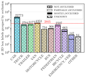
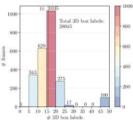
[Object classes including occlusion level. ] [Labeled 3D box labels per frame. ] [Rotations of 3D box labels. ]

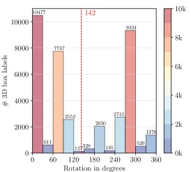
Figure 2: The A9-I Dataset consists of $38,045$ 3D box labels after data fusion, where the CAR class is dominant and $78.2\%$ of the objects are occlusion-free. The 3D box labels show different rotations, which is due to the road traffic in an intersection.

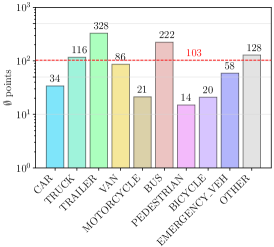
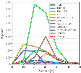
[Average number of points per class. ] [Number of points grouped by distance. ] [Number of points in a 3D box label. ]

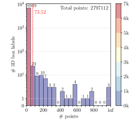
Figure 3: As expected, there is a causality between the dimensions of road users and the number of points. Most classes have the highest number of points at a distance between $10$ to $30$ meters. On average, each 3D box label contains $73.52$ points.

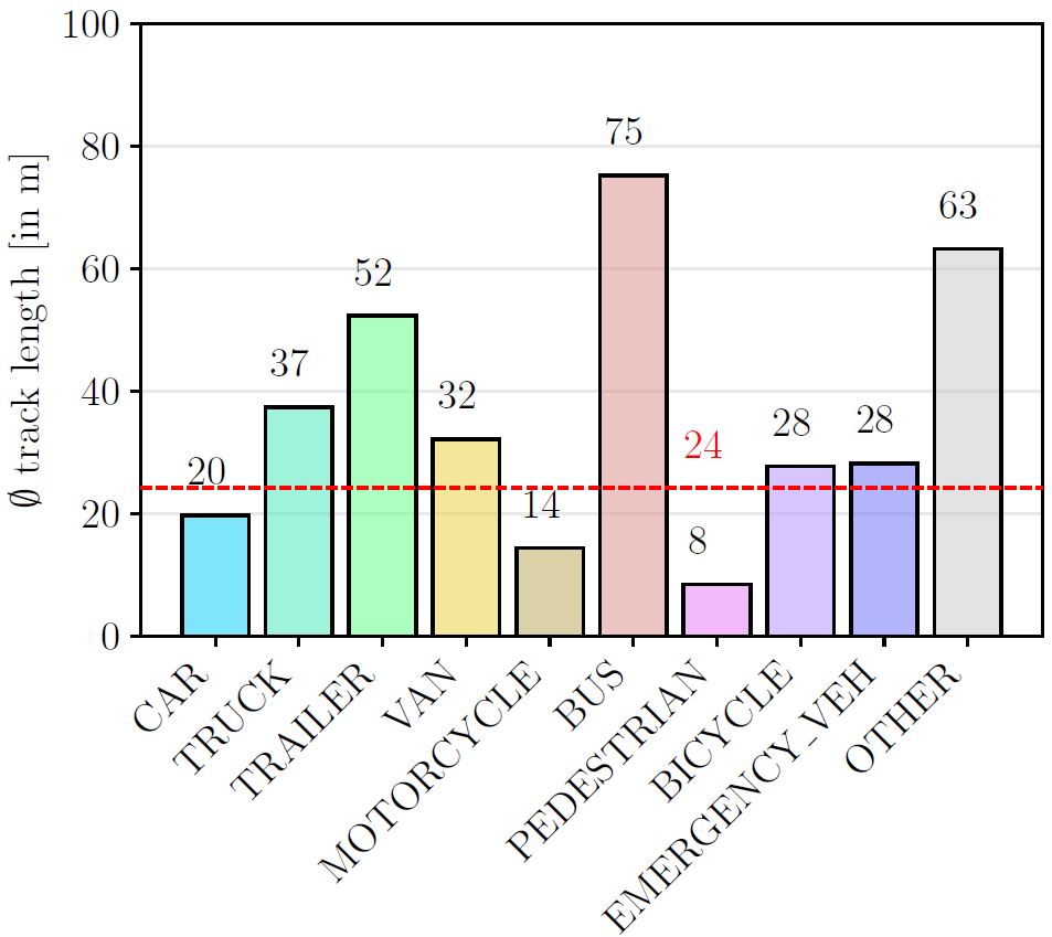
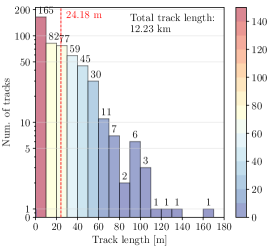
[Average track length per class. ] [Distribution of the several track lengths. ] [Visualization of tracks in BEV. ]

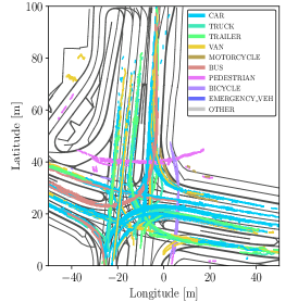
Figure 4: The 3D box label of each traffic participant has always received the same tracking ID in successive frames in a sequence. The average track length is $24.18~{}\text{m}$. In total, our 3D box labels have a track length of $12.23~{}\text{km}$.

We suggest a split into training ($80\%$), validation ($10\%$), and test set ($10\%$). The test set is made up of a continuous sequence with track IDs, as well as randomly sampled frames from four different scenarios and daytimes. We sample frames using stratified sampling to create a balanced dataset among sensor types, weather scenarios, and day times. To prevent overfitting, we do not publish our test set labels.

III-D Data Statistics

In total, we provide $4,800$ labeled LiDAR point cloud frames sampled from four different sequences. Here, $57,406$ 3D objects ($506$ unique objects) were annotated with $273,861$ object attributes. After fusing the labels from both LiDARs we get $38,045$ registered 3D objects ($482$ unique objects) with $171,045$ attributes. The following statistics refer to the fusion result with the complete dataset inclusive of training, validation, and test set. In Table II, we can see an overview of the registered 3D box labels.

TABLE II: The total number of labels, average dimensions in meters, and the average number of 3D LiDAR points among all classes.

Class	#Labels	$\diameter$Length	$\diameter$Width	$\diameter$Height	$\diameter$Points
Car	22,773	4.27	1.91	1.59	34.03
Truck	2,704	3.11	2.90	3.43	116.87
Trailer	3,177	10.19	3.12	3.65	328.36
Van	4,353	6.35	2.52	2.47	86.11
Motorcycle	734	1.90	0.83	1.60	21.23
Bus	908	12.65	2.95	3.27	222.36
Pedestrian	2,507	0.80	0.73	1.72	14.98
Bicycle	663	1.57	0.74	1.72	20.95
Emergency Vehicle	142	6.72	2.35	2.35	58.95
Other	84	5.28	1.92	1.90	128.17
Total	38,045	-	-	-	103.20

A deep dive into distribution of the labels of our A9-I Dataset is provided in Figure 2. Here, the distribution of the ten object classes is shown. The vehicle class CAR is dominant, followed by the classes TRUCK, TRAILER, VAN, and PEDESTRIAN, which occur in roughly the same order of magnitude. The classes MOTORCYCLE, BUS, BICYCLE, EMERGENCY VEHICLES, and OTHER are present in a slightly smaller number. Since we have annotated the occlusion level for each 3D box label, we come to the result that $78.2\%$ were classified as NOT_OCCLUDED, $16.1\%$ as PARTIALLY_OCCLUDED, $0.8\%$ as MOSTLY_OCCLUDED, and $4.9\%$ were classified as UNKNOWN (not labeled). It can also be seen that most of the labeled frames contain between $15$ and $20$ labeled 3D boxes. In 100 frames, there are even between $45$ and $50$ labeled 3D objects. Furthermore, the A9-I includes significantly more variations in the maneuvers of road users at the intersection, as compared to our previous work [14]. We can see three peaks where vehicles are moving to the south, north and east direction of the intersection. Vehicles moving between south and north are indicated by the peaks around $90$ and $270$ degrees. The smaller peaks adjacent to the main peaks correspond to turning maneuvers, such as right or left turns.

The labels are based on the LiDAR point clouds. In Figure 3, we performed a detailed analysis of the points concerning the labeled classes, of the individual distances of the points concerning the labeled classes, and of the distribution of the points. Firstly, as expected, the correlation between the average number of points and the average size of the class can be observed. Here, the TRAILER class, which has the highest height, also has the highest average number of points, followed by the BUS class, which is the longest. Conversely, the PEDESTRIAN class, which has the smallest size, has the lowest average number of points. Second, in general, due to the elevated position of the LiDARs, the field of view only starts to have an effect from about $10~{}\text{m}$ onwards. Most classes have the highest number of points at a distance between $10~{}\text{m}$ to $30~{}\text{m}$. Interestingly, the class TRAILER has the highest average number of points at a distance between $15~{}\text{m}$ and $20~{}\text{m}$. With increasing distance, the average number of points is naturally declining. Lastly, all 3D box labels have a total of $2,797,112$ points. According to the distribution of the number of points per 3D box label, most of the boxes have a maximum of about $50$ points. However, the 3D box labels have on average $73.52$ points per object.

In addition to the statistics about the labels and the underlying point clouds, we also analysed the calculated tracks, see Figure 4. We were able to determine these trivially since the same tracking ID was selected for each consecutive frame when marking the 3D box labels. The average track length in our A9-I Dataset is $24.18~{}\text{m}$. Here, the class BUS is very dominant with an average track length of $75~{}\text{m}$. The reason for this is because, firstly, the buses are very visible, and secondly, completely cross the intersection. All in all, the full dataset contains $506$ unique objects (3D box labels) with a total track length of $12.23~{}\text{km}$ with a maximum track length of $162.87~{}\text{m}$. Thus, our A9 Intersection Dataset can also be used to handle issues regarding tracking that are addressed by [22].

III-E A9-Devkit

To work with our A9-I Dataset, we provide the A9 Development Kit: https://github.com/providentia-project/a9-dev-kit. It contains a dataset loader to load images, point clouds, labels, and calibration data. Furthermore, we provide a converter from OpenLABEL to multiple different dataset formats like KITTI, COCO, YOLO, and the other way round. We follow the .json-based OpenLABEL standard [21] from the ASAM organization for the label structure. Some pre-processing scripts transform and filter the raw point cloud .pcd ASCII data into binary data to reduce the file size and make it compatible with point cloud loaders. In addition, a point cloud registration module can merge multiple point clouds to increase the point density. Finally, we provide a data visualization module to project the point clouds and labels into the camera images.

IV EVALUATION

TABLE III: Evaluation results on the A9-I Dataset test set (N=North, S=South, EF=Early Fusion, LF=Late Fusion).
                                                                                                                                                 We report the $mAP_{3D@0.1}$ results for the following six classes: Car, Truck, Bus, Motorcycle, Pedestrian, Bicycle. According to [23], we crop the dataset into three subsets: A9-I-south1 (Camera_South1), A9-I-south2 (Camera_South2), and A9-I-full (Camera_full).

FOV	Model	Sensor Modality	$\boldsymbol{mAP_{3D}}$
			Easy	Mod.	Hard	Overall
Camera_S1	MonoDet3D[23]	Camera_S1	43.27	13.28	2.16	19.57
Camera_S1	PointPillars⋆[24]	LiDAR_N	76.19	34.58	30.00	46.93
Camera_S1	PointPillars⋆[24]	LiDAR_S	46.35	41.05	24.16	37.18
Camera_S1	PointPillars⋆[24]	EF(LiDAR_N + LiDAR_S)	75.81	47.66	42.16	55.21
Camera_S1	InfraDet3D[23]	LF(Camera_S1 + EF(LiDAR_N + LiDAR_S))	67.08	31.38	35.17	44.55
Camera_S2	MonoDet3D[23]	Camera_S2	16.82	27.87	26.67	23.78
Camera_S2	PointPillars⋆[24]	LiDAR_N	45.26	27.26	26.24	32.92
Camera_S2	PointPillars⋆[24]	LiDAR_S	26.27	38.24	13.16	25.89
Camera_S2	PointPillars⋆[24]	EF(LiDAR_N + LiDAR_S)	38.92	46.60	43.86	43.13
Camera_S2	InfraDet3D[23]	LF(Camera_S2 + EF(LiDAR_N + LiDAR_S))	58.38	19.73	33.08	37.06
Camera_full	MonoDet3D[23]	LF(Camera_S1 + Camera_S2)	19.05	24.12	25.55	22.91
Camera_full	PointPillars⋆[24]	LiDAR_N	76.04	26.03	20.60	40.89
Camera_full	PointPillars⋆[24]	LiDAR_S	38.82	32.83	10.93	27.53
Camera_full	PointPillars⋆[24]	EF(LiDAR_N + LiDAR_S)	70.53	44.20	39.04	51.25
Camera_full	InfraDet3D[23]	LF(LF(Camera_S1+Camera_S2) + LF(LiDAR_N+LiDAR_S))	47.27	26.15	19.71	31.04
Camera_full	InfraDet3D[23]	LF(LF(Camera_S1+Camera_S2) + EF(LiDAR_N+LiDAR_S))	64.30	23.83	26.05	38.06
⋆PointPillars inference score threshold is set to 0.3.

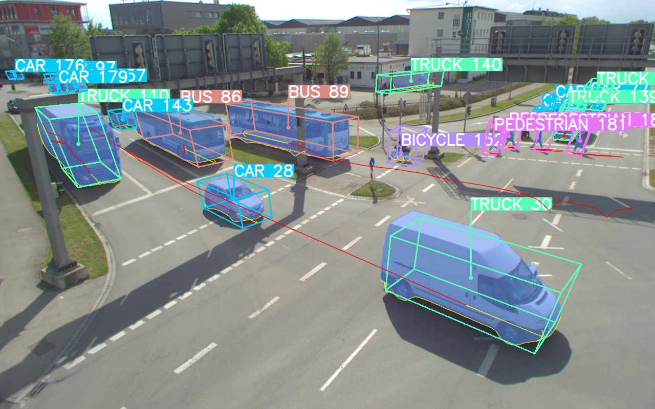
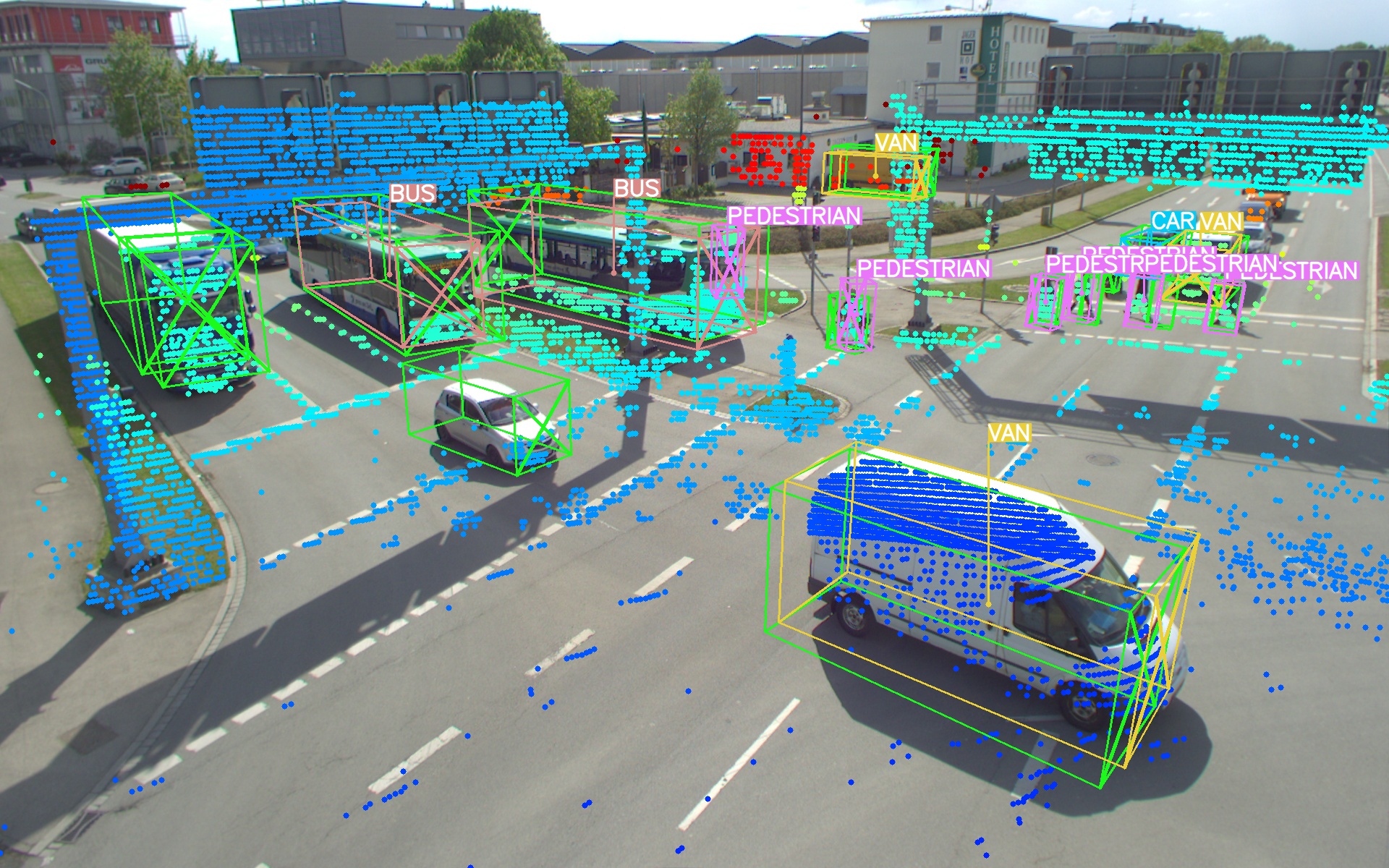
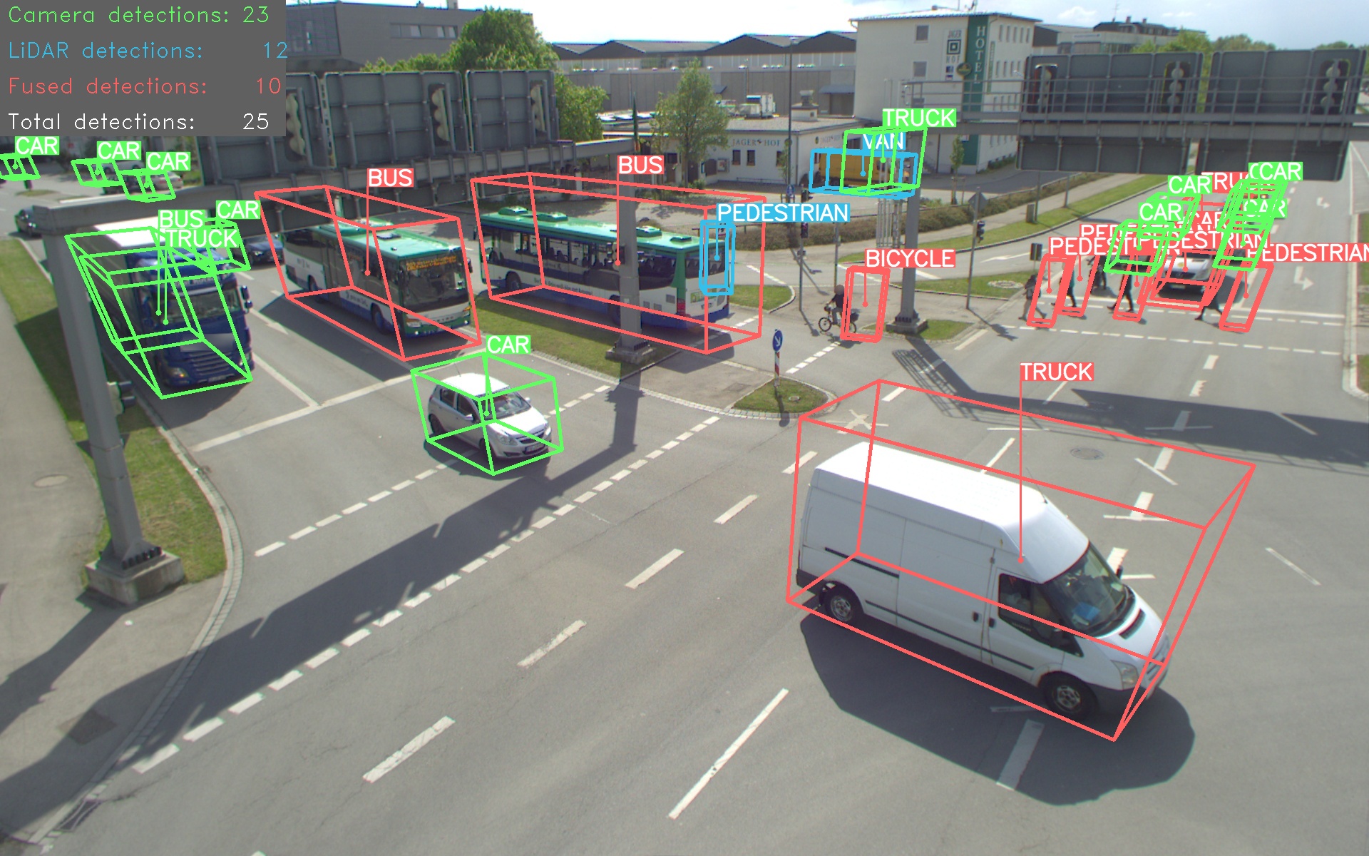
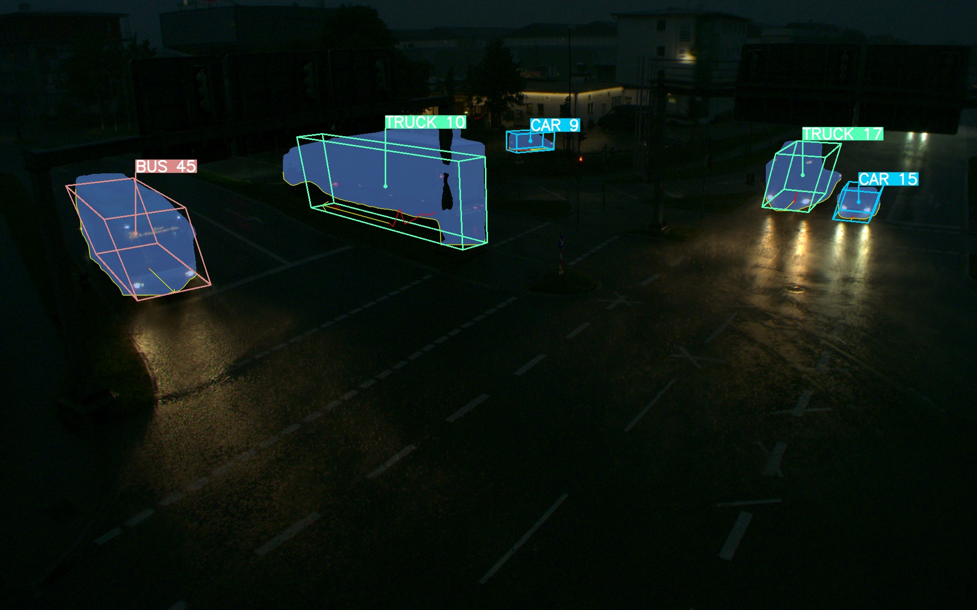
(a) MonoDet3D

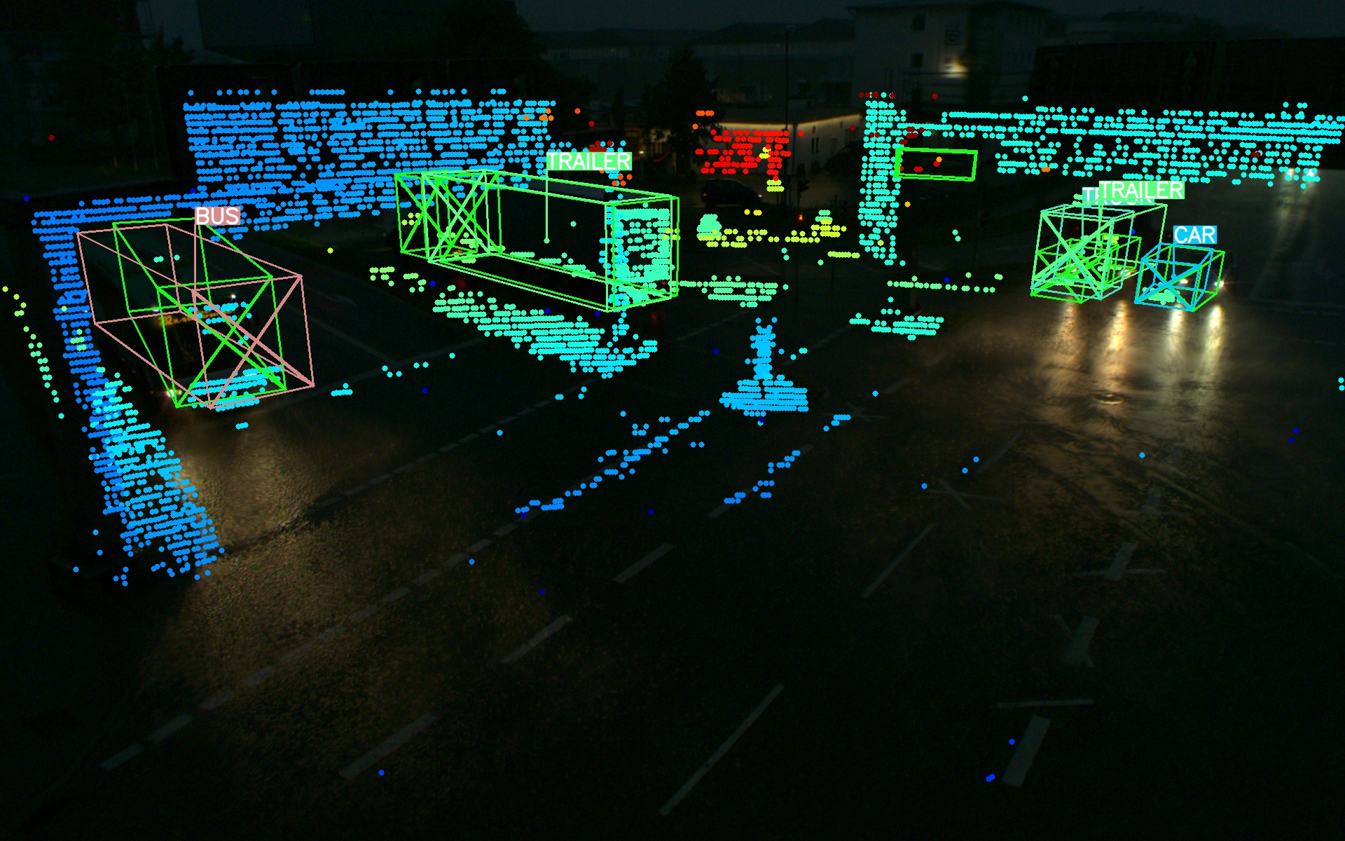
(b) PointPillars

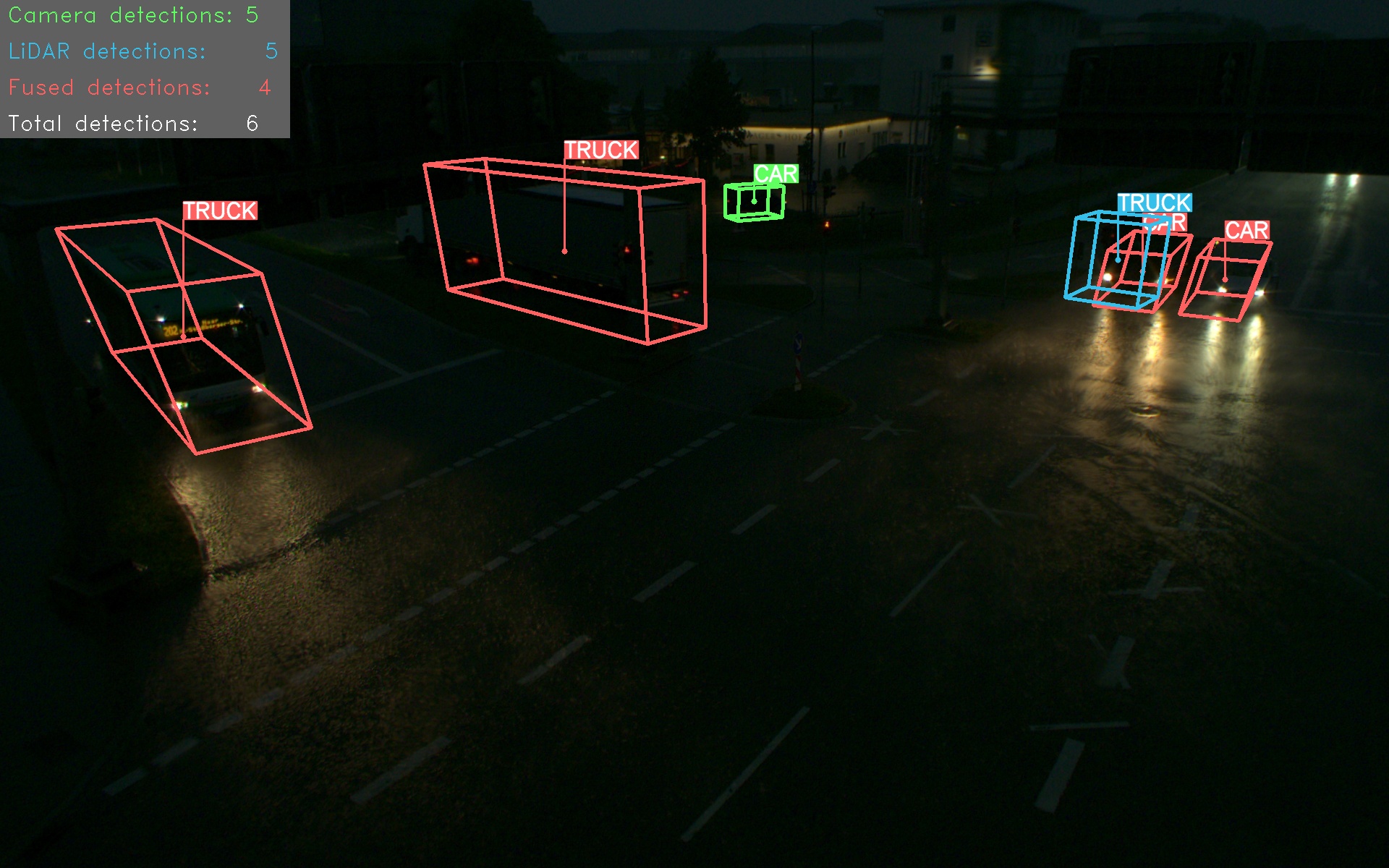
(c) InfraDet3D

Figure 5: Qualitative results on the test sequence of the three baselines: MonoDet3D (camera-only), PointPillars (LiDAR-only) and InfraDet3D (fusion) during the day (top row) and the night time (bottom row). Detections for MonoDet3D and PointPillars are colored by their class color. The fusion results of the InfraDet3D model are shown in red (fused detections), green (unmatched camera detections), and blue (unmatched LiDAR detections).

In our study, we conducted a comparative analysis of monocular camera and LiDAR 3D object detection with early and late fusion. In our first evaluation experiment, we used our MonoDet3D [23] 3D object detector that takes camera images as input. It transforms the 2D instance masks into 3D bottom contours by using extrinsic calibration data. Our augmented L-Shape-Fitting algorithm extracts the dimensions and calculates the rotation for each object. In our second experiment, we used PointPillars [24] and trained the model from scratch on all classes of our camera field of views Camera_south1, Camera_south2, and full. In the last experiment, we evaluate our multi-modal InfraDet3D [23] detector, which incorporates a late fusion approach, leveraging the Hungarian algorithm to establish correspondences between detections obtained from the MonoDet3D and PointPillars baselines. For all these experiments, we provide post-processing scripts in our A9-Devkit for early data fusion, and cropping the point cloud labels to fit the mentioned field of view.

We evaluated each detector on three difficulty levels Easy, Moderate, and Hard, see Table III. The Hard category contains objects with a distance over $50~{}\text{m}$, objects that are mostly occluded, or objects that have less than 20 points within the 3D box. Partially occluded objects with a distance of $40~{}\text{to}~{}50~{}\text{m}$, and 20 to 50 points are part of the Moderate category. Lastly, the Easy category contains objects that are not occluded, less than $40~{}\text{m}$ away, and contain more than 50 points. As a quantitative metric, we used the mean Average Precision (mAP) to evaluate the performance. The overall mAP is the average of Easy, Moderate, and Hard.

The advantage of using a monocular setup is a better detection of small objects such as pedestrians. On the other side, a LiDAR detector can detect objects during nighttime. The combination of LiDAR and the camera through late fusion techniques can significantly enhance the overall performance. In this work, we were able to confirm this assumption in our evaluation. We achieved the best detection results with the LiDAR_North modality and the InfraDet3D model in the Easy difficulty level. Interestingly, the early fusion approach with PointPillars consistently achieves the best performance in all subsets at Moderate difficulty level. The better performance of PointPillars and InfraDet3D over the MonoDet3D shows the strengths of the LiDAR sensor in comparison to a camera. Mostly, the late fusion of LiDAR and the camera provided better overall results than a single LiDAR detector. Moreover, the combination of early fusion between LiDAR sensors with camera sensors via late fusion, which combines the advantages of both sensor modalities, gives consistently robust results. A visual representation of the qualitative results is provided in Figure 5.

V CONCLUSIONS

In this work we extended the A9 Dataset with labeled data of an intersection. We provided 3D box labels from elevated road side sensors. Two synchronized cameras and LiDARs were used to record challenging traffic scenarios. Our data was labeled by experienced experts. As all sensors were calibrated to each other, we can use the 3D bounding box point cloud labels to perform Monocular 3D object detection. In total, our dataset contains $4.8\text{k}$ RGB images and $4.8\text{k}$ LiDAR point cloud frames with $57.4\text{k}$ high-quality labeled 3D boxes, partitioned into ten object classes of traffic participants. We offered a comprehensive statistics of the labels including their occlusion levels, the number of points grouped by class category and distance, and an extensive analysis of the labeled tracks. In our evaluation experiments, we provided three baselines for the perception task of 3D object detection: A camera, a LiDAR and a multi-modal camera-LiDAR combination. With these experiments, we were able to show the potential of our dataset for your 3D perception tasks.

For future work, we plan to create and publish more ground truth labels based on the presented camera images which can support more evaluation methods for our data fusion algorithm. Furthermore, the publication of further labeled sensor data with specific traffic scenarios, e.g. accidents, as well as the usage of other sensor modalities is also on our agenda.

References

- [1] A. Geiger, P. Lenz, C. Stiller, and R. Urtasun, “Vision meets robotics: The kitti dataset,” The International Journal of Robotics Research, vol. 32, no. 11, pp. 1231–1237, 2013.
- [2] Marius Cordts, Mohamed Omran, Sebastian Ramos, Timo Rehfeld, Markus Enzweiler, Rodrigo Benenson, Uwe Franke, Stefan Roth, and Bernt Schiele, “The cityscapes dataset for semantic urban scene understanding.” [Online]. Available: https://www.cv-foundation.org/openaccess/content_cvpr_2016/papers/Cordts_The_Cityscapes_Dataset_CVPR_2016_paper.pdf
- [3] R. Krajewski, J. Bock, L. Kloeker, and L. Eckstein, “The highd dataset: A drone dataset of naturalistic vehicle trajectories on german highways for validation of highly automated driving systems,” in 2018 IEEE Intelligent Transportation Systems Conference. Piscataway, NJ: IEEE, 2018, pp. 2118–2125.
- [4] H. Caesar, V. Bankiti, A. H. Lang, S. Vora, V. E. Liong, Q. Xu, A. Krishnan, Y. Pan, G. Baldan, and O. Beijbom, “nuscenes: A multimodal dataset for autonomous driving,” in Proceedings of the IEEE/CVF conference on computer vision and pattern recognition, 2020, pp. 11 621–11 631.
- [5] P. Sun, H. Kretzschmar, X. Dotiwalla, A. Chouard, V. Patnaik, P. Tsui, J. Guo, Y. Zhou, Y. Chai, B. Caine et al., “Scalability in perception for autonomous driving: Waymo open dataset,” in Proceedings of the IEEE/CVF conference on computer vision and pattern recognition, 2020, pp. 2446–2454.
- [6] J. Bock, R. Krajewski, T. Moers, S. Runde, L. Vater, and L. Eckstein, “The ind dataset: A drone dataset of naturalistic road user trajectories at german intersections,” in 2020 IEEE Intelligent Vehicles Symposium (IV). IEEE, 2020, pp. 1929–1934.
- [7] R. Krajewski, T. Moers, J. Bock, L. Vater, and L. Eckstein, “The round dataset: A drone dataset of road user trajectories at roundabouts in germany,” in 2020 IEEE 23rd International Conference on Intelligent Transportation Systems (ITSC). Piscataway, NJ: IEEE, 2020, pp. 1–6.
- [8] T. Moers, L. Vater, R. Krajewski, J. Bock, A. Zlocki, and L. Eckstein, “The exid dataset: A real-world trajectory dataset of highly interactive highway scenarios in germany,” in 2022 IEEE Intelligent Vehicles Symposium (IV). Piscataway, NJ: IEEE, 2022, pp. 958–964.
- [9] L. Gressenbuch, K. Esterle, T. Kessler, and M. Althoff, “Mona: The munich motion dataset of natural driving,” in 2022 IEEE 25th International Conference on Intelligent Transportation Systems (ITSC). IEEE, 2022, pp. 2093–2100.
- [10] H. Yu, Y. Luo, M. Shu, Y. Huo, Z. Yang, Y. Shi, Z. Guo, H. Li, X. Hu, J. Yuan et al., “Dair-v2x: A large-scale dataset for vehicle-infrastructure cooperative 3d object detection,” in Proceedings of the IEEE/CVF Conference on Computer Vision and Pattern Recognition, 2022, pp. 21 361–21 370.
- [11] H. Wang, X. Zhang, Z. Li, J. Li, K. Wang, Z. Lei, and R. Haibing, “Ips300+: a challenging multi-modal data sets for intersection perception system,” in 2022 International Conference on Robotics and Automation (ICRA). IEEE, 2022, pp. 2539–2545.
- [12] X. Ye, M. Shu, H. Li, Y. Shi, Y. Li, G. Wang, X. Tan, and E. Ding, “Rope3d: The roadside perception dataset for autonomous driving and monocular 3d object detection task,” in Proceedings of the IEEE/CVF Conference on Computer Vision and Pattern Recognition, 2022, pp. 21 341–21 350.
- [13] S. Busch, C. Koetsier, J. Axmann, and C. Brenner, “Lumpi: The leibniz university multi-perspective intersection dataset,” in 2022 IEEE Intelligent Vehicles Symposium (IV). IEEE, 2022, pp. 1127–1134.
- [14] C. Creß, W. Zimmer, L. Strand, M. Fortkord, S. Dai, V. Lakshminarasimhan, and A. Knoll, “A9-dataset: Multi-sensor infrastructure-based dataset for mobility research,” in 2022 IEEE Intelligent Vehicles Symposium (IV), 2022, pp. 965–970.
- [15] C. Creß, Z. Bing, and A. C. Knoll, “Intelligent transportation systems using external infrastructure: A literature survey.” [Online]. Available: https://arxiv.org/pdf/2112.05615
- [16] J. Bock, R. Krajewski, T. Moers, S. Runde, L. Vater, and L. Eckstein, “The ind dataset: A drone dataset of naturalistic road user trajectories at german intersections,” in 2020 IEEE Intelligent Vehicles Symposium (IV). Piscataway, NJ: IEEE, 2020, pp. 1929–1934.
- [17] A. Krämmer, C. Schöller, D. Gulati, V. Lakshminarasimhan, F. Kurz, D. Rosenbaum, C. Lenz, and A. Knoll, “Providentia-a large-scale sensor system for the assistance of autonomous vehicles and its evaluation,” Journal of Field Robotics, pp. 1156–1176, 2022.
- [18] “Projekt providentia++,” 2022. [Online]. Available: https://innovation-mobility.com/projekt-providentia/
- [19] Y. Chongjian, X. Liu, X. Hong, and F. Zhang, “Pixel-level extrinsic self calibration of high resolution lidar and camera in targetless environments,” IEEE Robotics and Automation Letters, vol. PP, pp. 1–1, 07 2021.
- [20] W. Zimmer, A. Rangesh, and M. Trivedi, “3d bat: A semi-automatic, web-based 3d annotation toolbox for full-surround, multi-modal data streams,” in 2019 IEEE Intelligent Vehicles Symposium (IV). IEEE, 2019, pp. 1816–1821.
- [21] N. Hagedorn, “OpenLABEL Concept Paper.” [Online]. Available: https://www.asam.net/project-detail/asam-openlabel-v100/
- [22] L. Strand, J. Honer, and A. Knoll, “Systematic error source analysis of a real-world multi-camera traffic surveillance system,” in 2022 25th International Conference on Information Fusion (FUSION). IEEE, 7/4/2022 - 7/7/2022, pp. 1–8.
- [23] W. Zimmer, J. Birkner, M. Brucker, H. T. Nguyen, S. Petrovski, B. Wang, and A. C. Knoll, “Infradet3d: Multi-modal 3d object detection based on roadside infrastructure camera and lidar sensors,” arXiv preprint arXiv:2305.00314, 2023.
- [24] A. H. Lang, S. Vora, H. Caesar, L. Zhou, J. Yang, and O. Beijbom, “Pointpillars: Fast encoders for object detection from point clouds,” in Proceedings of the IEEE/CVF conference on computer vision and pattern recognition, 2019, pp. 12 697–12 705.