Two sided ergodic singular control and
mean field game for diffusions

Abstract

Consider two independent controlled linear diffusions with the same dynamics and the same ergodic controls, the first corresponding to an individual player, the second to the market. Let us also consider a cost function that depends on the first diffusion and the expectation of the second one. In this framework, we study the mean-field game consisting in finding the equilibrium points where the controls chosen by the player to minimize an ergodic integrated cost coincide with the market controls. We first show that in the control problem, without market dependence, the best policy is to reflect the process within two boundaries. We use these results to get criteria for the optimal and market controls to coincide (i.e., equilibrium existence), and give a pair of nonlinear equations to find these equilibrium points. We also get criteria for the existence and uniqueness of equilibrium points for the mean-field games under study. These results are illustrated through several examples where the existence and uniqueness of the equilibrium points depend on the values of the parameters defining the underlying diffusion.

Keywords: Ergodic singular control, Diffusions, Mean field games, Nash equilibrium

1 Introduction

In recent years, mean-field game theory has emerged as a powerful framework for modeling the behavior of large populations of interacting agents in a stochastic environment. This interdisciplinary field lies at the intersection of mathematics, economics, and engineering, offering deep insights into complex systems characterized by strategic interactions. Mean field game models have found applications in various domains, including for instance, finance, energy systems (Carmona, 2020), or traffic management and social dynamics (Festa and Göttlich, 2018). The study of mean field games typically involves analyzing the behavior of a large number of identical agents who aim to optimize their individual objectives while accounting for the average behavior of the population.

In the present paper we incorporate a mean-field game model in the two-sided ergodic singular control problem for Itô diffusions, giving new insights in the general framework described above. The control problem has been extensively studied and analyzed in the literature, see for example Alvarez and Shepp (1998), Hening, Nguyen, Ungureanu and Wong (2017), and Lande and Engen and Sæther (1994). Regarding applied work, we mention studies focusing on cash flow management that explore optimal dividend distribution, recapitalization, or a combination of both while considering risk neutrality. These investigations also fall under the domain of singular control problems, see for instance Asmussen and Taksar (1997), H$\o$jgaard and Taksar (2001), Jeanblanc-Picqué and Shiryaev (1995), Paulsen (2008), Peura and Keppo (2006), and Shreve et al. (1984). Recently, there have been advances in the more particular case where the nature of the problem makes controls of bounded variation to appear naturally, also called two-sided average singular control ergodic problem, see for example the works by Kunwai et al. (2022) and Alvarez (2018). In this second paper, the author restricted the problem to reflecting barriers, that is, the policies allowed are the ones that reflect in thresholds.

Our main objective is to investigate the interplay between two-sided ergodic singular control and mean field game theory under the framework proposed by Alvarez (2018), considering a class of more general controls. Our results indicate how individual agents can make strategic decisions in the presence of a large population while accounting for the impact of their own control on the average behavior. To achieve our goals, we postulate a verification theorem in the form of a Hamilton-Jacobi-Bellman equation and use the ergodic properties of the controlled processes to turn the mean-field game into an analytic problem. As a consequence, we obtain necessary and sufficient conditions for the existence of mean-field game equilibrium points, and, for more restricted families of cost functions, uniqueness for thresholds strategies. Finally, we define an $N$-player problem and prove that it approximates our ergodic mean field game as the number of players goes to infinity. This means that the mean-field equilibrium is an approximate Nash equilibrium for the $N$-player game.

The rest of the paper is organized as follows. In Section 2 we study the control problem. After introducing the necessary tools, we state and prove the main result of the section, i.e. the optimality of reflecting controls obtained within the class of càdlàg controls. In Section 3 we consider the mean-field game problem. It adds the complexity of a two-variable cost function where the second variable represents the market. The main result consists of a set of conditions for the existence and uniqueness of equilibrium strategies, containing also a particular analysis when the cost function is multiplicative. Section 4 presents three examples that illustrate these results. Section 5 contains approximation results when the market consists of $N$ players. A final appendix includes some auxiliary computations corresponding to the last two sections.

2 Control problem

In this section, we consider the one-player control problem. We first recall results obtained by Alvarez (2018) that play a fundamental rôle along the paper. These results consist in the determination of optimal control levels in an ergodic framework for a diffusion within the class of reflecting controls. After this, we prove that the optimum levels found in Alvarez (2018) give in fact the optimum controls within the wider class of finite variation càdlàg controls.

Let us consider a filtered probability space $(\Omega,P,\{\mathcal{F}_{t}\},\mathcal{F})$ that satisfy the usual assumptions. In order to define the underlying diffusion consider the measurable functions $\mu\colon\mathbb{R}\to\mathbb{R}$ and $\sigma\colon\mathbb{R}\to\mathbb{R}$ assumed to be locally Lipschitz. Under these conditions the stochastic differential equation

$$dX_{t}=\mu(X_{t})dt+\sigma(X_{t})dW_{t},\ X_{0}=x_{0}$$ (1)

has a unique strong solution up to an explosion time, that we denote $X=\{X_{t}\colon t\geq 0\}$ (see Protter (2005, Theorem V.38)). Observe that our framework includes quadratic coefficients. Alternatively, our results can be formulated in the framework of weak solutions as in Alvarez (2018).

As usual, we define the infinitesimal generator of the process $X$ as

$$\mathcal{L}_{X}=\frac{1}{2}\sigma^{2}(x)\frac{\displaystyle d^{2}}{\displaystyle d^{2}x}+\mu(x)\frac{\displaystyle d}{\displaystyle dx}.$$

We denote the density of the scale function $S(x)$ w.r.t the Lebesgue measure as

$$S^{\prime}(x)=\exp\left(-\int^{x}\frac{2\mu(u)}{\sigma^{2}(u)}du\right),$$

and the density of the speed measure $m(x)$ w.r.t the Lebesgue measure as

$$m^{\prime}(x)=\frac{2}{\sigma^{2}(x)S^{\prime}(x)}.$$

As mentioned above, the underlying process is controlled by a pair of processes, the admissible controls, that drive it to a convenient region, defined below.

Definition 2.1.

An admissible control is a pair of non-negative $\{\mathcal{F}_{t}\}$-adapted processes $(D,U)=(\{D_{t}\}_{t\geq 0},\{U_{t}\}_{t\geq 0})$ such that:

• Each process $D,U\colon\Omega\times\mathbb{R}_{+}\rightarrow\mathbb{R}_{+}$ is right continuous and non decreasing almost surely.

• For each $t\geq 0$ the random variables $U_{t}$ and $D_{t}$ have finite expectation.

• For every $x\in\mathbb{R}$ the stochastic differential equation

  $$dX^{(D,U)}_{t}:=\mu(X^{(D,U)}_{t})dt+\sigma(X^{(D,U)}_{t})dW_{t}-dD_{t}+dU_{t},\quad X_{0}=x$$ (2)

  has a unique strong solution with no explosion in finite time.

We denote by $\mathcal{A}$ the set of admissible controls.

Note that condition (iii) is satisfied, for instance, when the coefficients are globally Lipschitz. (See the remark after Theorem V.38 in Protter (2005).) Observe also that condition (ii) is not a real restriction, as, for instance, the integral in the cost function $G(x)$ in (3) that we aim to minimize, in case of having infinite expectations, is infinite. A relevant sub-class of admissible controls is the set of reflecting controls.

Definition 2.2.

For $a<b$ denote by $X^{a,b}=\{X^{a,b}_{t}\colon t\geq 0\}$ the strong solution of the stochastic differential equation with reflecting boundaries at $a$ and $b$:

$$dX^{a,b}_{t}=\mu(X^{a,b}_{t})dt+\sigma(X^{a,b}_{t})dW_{t}-dD^{b}_{t}+dU^{a}_{t},\qquad X_{0}=x.$$

Here $\{D^{b}_{t}\},\{U^{a}_{t}\}$ are non-decreasing processes that increase, respectively, only when the solution visits $a$ or $b$. As the above equation has a strong solution that does not explode in finite time (see (Saisho, 1987, Theorem 5.1)), the pair $(\{U^{a}_{t}\},\{D^{b}_{t}\})$ belongs to $\mathcal{A}$, and are called reflecting controls. If $x\notin(a,b)$ we define the policy by sending the process to a point inside the interval at time $t=0$.

We introduce below the cost function to be considered with some natural assumptions on its behavior.

Assumptions 2.3.

Consider a continuous cost function $c\colon\mathbb{R}\rightarrow\mathbb{R}_{+}$ and two positive values $q_{u},q_{d}$. Assume that

$$c(x) \geq c(0)\geq 0\ \forall x\in\mathbb{R},$$

$$c(x) +K\geq\alpha|x|.$$

where $K$ and $\alpha$ are positive constants. Define the maps

$$\pi_{1}(x)=c(x)+q_{d}\mu(x),\hskip 28.45274pt\pi_{2}(x)=c(x)-q_{u}\mu(x)$$

and assume that:

• There is a unique real number $x_{i}^{0}=\operatorname*{arg\,min}\{\pi_{i}(x)\}$ so that $\pi_{i}(\cdot)$ is decreasing on $(-\infty,x_{i}^{0})$ and increasing on $(x_{i}^{0},\infty)$ for $i=1,2$.

• It hold that

  $$\lim_{x\rightarrow\infty}\pi_{1}(x)=\lim_{x\rightarrow-\infty}\pi_{2}(x)=\infty.$$

Definition 2.4.

We define the ergodic cost function as

$$G(x)=\inf_{(D,U)\in\mathcal{A}}\limsup_{T\to\infty}\frac{1}{T}\operatorname{\mathbf{E}}_{x}\left(\int_{0}^{T}c(X^{D,U}_{s})ds+q_{u}U_{T}+q_{d}D_{T}\right),$$ (3)

where $(D,U)$ is a pair of admissible controls in $\mathcal{A}$.

The existence of a unique pair of optimal controls within the class of reflecting controls was obtained by Alvarez (2018), from where we borrow the notation and assumptions. More precisely the author proved the next two results:

Theorem 2.5 (Alvarez (2018)).

Assume 2.3. Then

(a) If $a<b$ then

$$\limsup_{T\rightarrow\infty}\frac{1}{T}\operatorname{\mathbf{E}}_{x}\left(\int_{0}^{T}c(X_{s}^{a,b})ds+q_{d}dD^{a}_{s}+q_{u}dU^{b}_{s}\right)\\ =\frac{1}{m(a,b)}\left[\int_{a}^{b}c(u)m(du)+\frac{q_{u}}{S^{\prime}(a)}+\frac{q_{d}}{S^{\prime}(b)}\right].$$

(b) There is an unique pair of points $a^{\ast}<b^{\ast}$ that satisfy the equations:

• $\pi_{1}(b^{\ast})=\pi_{2}(a^{\ast})$,

• $\int_{a^{\ast}}^{b^{\ast}}\left(\pi_{1}(t)-\pi_{1}(b^{\ast})\right)m(dt)+\frac{\displaystyle q_{d}+q_{u}}{\displaystyle S^{\prime}(a^{\ast})}=0$.

Furthermore, the pair $(a^{\ast},b^{\ast})$ minimizes the expected long-run average cost within the class of reflecting policies.

Remark 2.6.

Condition (i) is obtained from the fact $X^{a,b}$ is stationary. Regarding equation (ii), it arises after differentiation in order to determine the minimum. Uniqueness of the solution is proved based on the properties of the cost function. See the details in Alvarez (2018).

2.1 Optimality within $\mathcal{A}$

Optimality within the class $\mathcal{A}$ of càdlàg controls requires further analysis. As expected, and mentioned in Alvarez (2018), the optimal controls within class $\mathcal{A}$ are the same controls found in the class of reflecting controls. An analogous result to the one presented below was obtained for non-negative diffusions when considering a maximization problem in which $q_{u}$ and $q_{d}$ have opposite signs in Haoyang et al. (2021) (see also Kunwai et al. (2022)).

More precisely, it is clear that

$$\inf_{a<b}\limsup_{T\rightarrow\infty}\frac{1}{T}\operatorname{\mathbf{E}}_{x}\left(\int_{0}^{T}c(X_{s}^{a,b})ds+q_{d}dD^{a}_{T}+q_{u}dU^{b}_{T}\right)\geq G(x).$$

Then, to establish the optimality within $\mathcal{A}$ it is necessary to obtain the other inequality. This task is carried out with the help of the solution of the free boundary problem (11) below, as done in Haoyang et al. (2021). The mentioned differences with this situation require different hypotheses and slightly different arguments.

Theorem 2.7 (Verification).

Consider a diffusion defined by (1), a pair of controls $(D,U)\in\mathcal{A}$ and a cost function satisfying Assumptions 2.3. Suppose that there exist a constant $\lambda\geq 0$ and a function $u\in C^{2}(\mathbb{R})$ such that

$$(\mathcal{L}_{X}u)(x)+c(x)\geq\lambda,\qquad-q_{u}\leq u^{\prime}(x)\leq q_{d},$$ (4)

and

$$\liminf_{T\rightarrow\infty}\frac{1}{T}\left|\operatorname{\mathbf{E}}_{x}(u(X^{D,U}(T)))\right|=0,\quad\text{for all $x\in\mathbb{R}$}.$$ (5)

Then, the ergodic cost function defined in (3) satisfies

$$G(x)\geq\lambda.$$ (6)

Proof.

Fix $T>0$. For each $n\geq 1$ define the stopping times

$$T_{n}=\inf\{t\geq 0\colon|X^{D,U}_{t}|\geq n\}\wedge T\nearrow T\quad a.s.$$

Using Itô formula for processes with jumps (observe that the diffusion $X$ is continuous but the controls can have jumps, and in consequence the controlled processes $X^{D,U}$ can have jumps),

$$u(X^{D,U}(T_{n})) =u(x)+\int_{0}^{T_{n}}u^{\prime}(X^{D,U}_{s-})dX^{D,U}_{s}$$

$$\quad+\frac{1}{2}\int_{0}^{T_{n}}u^{\prime\prime}(X^{D,U}_{s-})d\langle(X^{D,U})^{c},(X^{D,U})^{c}\rangle_{s}$$

$$\quad+\sum_{s\leq T_{n}}\left(u(X^{D,U}_{s})-u(X^{D,U}_{s-})-u^{\prime}(X^{D,U}_{s-})\bigtriangleup X^{D,U}_{s}\right).$$ (7)

The r.h.s in (2.1) can be rewritten as

$$u(x) +\int_{0}^{T_{n}}(\mathcal{L}_{X}u)(X^{D,U}_{s-})ds-\int_{0}^{T_{n}}\mu(X^{D,U}_{s-})u^{\prime}(X^{D,U}_{s-})ds$$

$$+\int_{0}^{T_{n}}u^{\prime}(X^{D,U}_{s-})dX^{D,U}_{s}$$

$$+\sum_{s\leq T_{n}}\left(u(X^{D,U}_{s})-u(X^{D,U}_{s-})-u^{\prime}(X^{D,U}_{s-})\bigtriangleup X^{D,U}_{s}\right).$$ (8)

Using the fact that $u^{\prime}(X^{D,U}_{s-})=u^{\prime}(X^{D,U}_{s})$ in a set of total Lebesgue measure in $[0,T]$ almost surely, and that $\bigtriangleup X^{D,U}_{s}=\bigtriangleup U_{s}-\bigtriangleup D_{s}$, we rewrite (2.1) as

$$u(x) +\int_{0}^{T_{n}}(\mathcal{L}_{X}u)(X^{D,U}_{s-})ds+\int_{0}^{T_{n}}u^{\prime}(X^{D,U}_{s-})\sigma(X^{D,U}_{s-})dW_{s}$$

$$+\int_{0}^{T_{n}}u^{\prime}(X^{D,U}_{s-})d(U_{s}-D_{s})$$

$$+\sum_{s\leq T_{n}}\left(u(X^{D,U}_{s})-u(X^{D,U}_{s-})-u^{\prime}(X^{D,U}_{s-})(\bigtriangleup U_{s}-\bigtriangleup D_{s})\right).$$ (9)

Therefore, denoting by $U_{s}^{c}$ and $D_{s}^{c}$ the continuous parts of the processes $U_{s}$ and $D_{s}$ respectively, and using the inequalities (4) in the hypothesis, we obtain

$$u(X^{D,U}(T_{n})) \geq u(x)+\lambda T_{n}-\int_{0}^{T_{n}}c(X^{D,U}_{s-})ds$$

$$\quad+\int_{0}^{T_{n}}u(X^{D,U}_{s-})\sigma(X^{D,U}_{s-})dW_{s}-\int_{0}^{T_{n}}q_{u}dU^{c}_{s}$$

$$\quad-\int_{0}^{T_{n}}q_{d}dD^{c}_{s}-\sum_{0\leq s\leq T_{n}}(\bigtriangleup D_{s}q_{d}+\bigtriangleup U_{s}q_{u})$$

$$=u(x)+\lambda T_{n}-\int_{0}^{T_{n}}c(X^{D,U}_{s-})ds+\int_{0}^{T_{n}}u(X^{D,U}_{s-})\sigma(X^{D,U}_{s-})dW_{s}$$

$$\quad-q_{u}U_{T_{n}}-q_{d}D_{T_{n}}.$$

Rearranging the terms above and taking the expectation we obtain

$$\operatorname{\mathbf{E}}_{x}(u(X^{D,U}(T_{n})))-u(x)+\\ \operatorname{\mathbf{E}}_{x}\left(\int_{0}^{T_{n}}c(X^{D,U}_{s-})ds+q_{u}U_{T_{n}}+q_{d}D_{T_{n}}\right)\geq\lambda\operatorname{\mathbf{E}}_{x}(T_{n}).$$ (10)

Taking first limit as $n$ tends to infinity, dividing then by $T$, and finally taking $\liminf$ as $T$ goes to infinity we obtain (6) concluding the proof of the verification theorem. ∎

Consideration of free boundary problems such as (4) in the framework of singular control problems can be found for example in Alvarez (2018), Haoyang et al. (2021), and Kunwai et al. (2022). In Alvarez (2018), the author studied the same problem of this section and used a free boundary problem to find some useful properties of optimal controls within the class of reflecting barriers. More precisely, under the same assumptions as above, to study the ergodic optimal control problem in the class of reflecting controls, the author considered the free boundary problem consisting of finding $a<b,\lambda$ and a function $u$ in $C^{2}(\mathbb{R})$ such that

$$\left\{\begin{aligned} (\mathcal{L}_{X}u)(x)+c(x)&=\lambda,&\text{for all $x\in(a,b)$},\\ u(x)&=q_{d}(x-b)+u(b),&\text{for all $x\geq b$},\\ u(x)&=q_{u}(a-x)+u(a),&\text{for all $x\leq a$}.\end{aligned}\right.$$ (11)

For this problem it is proved (see Remark 2.4 in Alvarez (2018)) that there exists a unique solution such that

$$-q_{d}\leq u^{\prime}(x)\leq q_{u},\ (\mathcal{L}_{X}u)(x)+c(x)\geq\lambda.$$

Here, similar to Kunwai et al. (2022), we use the results obtained in Alvarez (2018) to get a suitable candidate to apply Theorem 2.7.

Theorem 2.8.

Consider a diffusion defined by (1) and a cost function satisfying Assumptions 2.3. Then, the reflecting controls with barriers given in (b) in Theorem 2.5 minimize the ergodic cost in (3) within the set $\mathcal{A}$ of admissible controls.

Proof.

Take $u$ as the solution of the free boundary problem (11) defined above. In view of condition (5), we need to prove that the infimum of the ergodic costs is reached in the set

$$\mathcal{B}:=\left\{(D,U)\in\mathcal{A},\liminf_{T\rightarrow\infty}\frac{1}{T}\left|\operatorname{\mathbf{E}}_{x}(u(X^{D,U}_{T}))\right|=0\right\}.$$

If $(D,U)\notin\mathcal{B}$ then there exists constants $L>0$ and $S>0$ such that

$$\frac{1}{s}\operatorname{\mathbf{E}}_{x}u(X^{D,U}_{s})>L,\quad\text{for all $s\geq S$}.$$

Using the fact that $u$ is a linear function in $(a,b)^{c}$ and that $-q_{u}\leq u^{\prime}(x)\leq q_{d}$ it follows that

$$\frac{1}{s}\operatorname{\mathbf{E}}_{x}|X^{D,U}_{s}|>\frac{L}{q_{d}+q_{u}}-\frac{|u(0)|}{s},\quad\text{for all $s\geq S$}.$$

We conclude that

$$\limsup_{T\to\infty}\frac{1}{T}\operatorname{\mathbf{E}}_{x}\left(\int_{0}^{T}c(X^{D,U}_{s})ds\right)\geq\limsup_{T\to\infty}\frac{1}{T}\int_{S}^{T}\operatorname{\mathbf{E}}_{x}(\alpha|X^{D,U}_{s}|+K)ds\geq\\ \limsup_{T\to\infty}\int_{S}^{T}\alpha(q_{d}+q_{u})^{-1}L\ ds+\frac{(K-|u(0)|)(T-S)}{T}=\infty.$$

Thus in the set $\mathcal{B}^{c}$ the infimum defined in (3) cannot be reached because if we take $\mathcal{B}^{c}$ instead of $\mathcal{A}$ in that equation then $G(x)=\infty$ for all $x\in\mathbb{R}$, concluding the proof. ∎

3 Mean Field Game Problem

As usual in the mean-field formulation, it is assumed that the cost function $C$ depends on two variables, i.e. $C=C(x,\mu)$. The first variable represents the state of the player $x$, and the second one is a probability measure $\mu$ that represents the aggregate of the rest of the players, referred as the market. For this kind of problem, there is a fixed measure valued function $\mu=\{\mu_{t}\}$ and the player tries to choose the best control $\alpha=\{\alpha_{t}\}$ belonging to a set $\mathcal{C}$ of stochastic processes (the set of admissible controls), in order to minimize a target function $J^{\mu}_{\alpha}$, that represents the average cost in the long run. It is common to solve these types of problems with the help of fixed point arguments (see for example Huang (2013) and Huang et al. (2004)) applied to a map of the form

$$\mu\rightarrow\mathcal{L}(X^{\mu}_{\alpha})$$

with $\mathcal{L}(X^{\mu}_{\alpha})$ the law of the state process controlled by $\alpha$ such that

$$\alpha\in\operatorname*{arg\,min}_{\beta\in\mathcal{C}}J^{\mu}_{\beta}.$$

3.1 Market evolution

In the case considered in this paper, we assume that the aggregate of players is modeled by a controlled diffusion $Y^{(D,U)}=\{Y^{(D,U)}_{t}\colon t\geq 0\}$. The definitions of $Y^{(D,U)}$ and $Y^{c,d}$ are analogous to the definitions of $X^{(D,U)}$ and $X^{a,b}$ respectively, in particular the coefficients of the respective stochastic differential equations and the class of admissible controls are the same. We further assume that the driving processes $\{Y_{t}\colon t\geq 0\}$ and $\{X_{t}\colon t\geq 0\}$ are independent.

Comparing this approach with the general formulation, the measure $\mu_{t}$ is the distribution of the random variable $Y^{D,U}_{t}$ that enters the cost function through an expectation, i.e.

$$C(x,\mu)=c\left(x,\int_{\mathbb{R}}f(y)d\mu\right),$$

where $f$ is a measurable function. We can then formulate this situation through the cost $c(x,y)$ that depends on an pair $(x,y)\in\mathbb{R}^{2}$. This allows us to use a more direct approach to find equilibrium points.

More precisely, if the expectation of the market diffusion $\operatorname{\mathbf{E}}_{y}(f(Y^{D,U}_{t}))$ has an ergodic limit $\ell=\operatorname{\mathbf{E}}_{y}(f(Y^{D,U}_{\infty}))$, applying the previous results, we know that the optimal controls for $X$ should be found in the class of reflecting controls (considering a one variable cost function of the form $c(\cdot,\ell)$). This is why we assume that the aggregate market diffusion is also controlled by reflection at some levels $c<d$, and expect to obtain an equilibrium point when the optimal levels $a<b$ that control the player’s diffusion coincide with $c<d$ (see Def. 3.3). Note that the question of the existence of equilibrium strategies beyond the class of reflecting controls is not addressed here.

As mentioned above, we consider a cost function of two variables, respectively the state of the player and the aggregate of players. The proposal to study the existence and uniqueness of equilibrium points begins with the application of Theorem 2.5 when the aggregate state is constant. The cost function becomes one-dimensional and the results in Alvarez (2018) can be applied. The requirements to apply these results in the mean field game formulation follow.

Assumptions 3.1.

Assume that $c\colon\mathbb{R}^{2}\rightarrow\mathbb{R}_{+}$ is a continuous function, and the positive constants $q_{u},q_{d}$ are the cost of the controls. Assume that, for each fixed $y\in\mathbb{R}$ there exist a value $x_{y}$ and positive constants $K_{y}$ and $\alpha_{y}$ such that

$$c(x,y)\geq c(x_{y},y)\geq 0,\qquad\text{for all $x\in\mathbb{R}$},$$

$$c(x,y)+K_{y}\geq\alpha_{y}|x|,\qquad\text{for all $x\in\mathbb{R}$}.$$

Define the maps

$$\pi_{1}(x,y):=c(x,y)+q_{d}\mu(x),\hskip 28.45274pt\pi_{2}(x,y)=c(x,y)-q_{u}\mu(x),$$

and assume that for each fixed $y\in\mathbb{R}$

• There exists a unique real number $x^{y}_{i}=argmin\{\pi_{i}(x,y)\colon x\in\mathbb{R}\}$ so that $\pi_{i}(\cdot,y)$ is decreasing on $(-\infty,x^{y}_{i})$ and increasing on $(x^{y}_{i},\infty)$, where $i=1,2$.

• The following limits hold:

  $$\lim_{x\rightarrow\infty}\pi_{1}(x,y)=\lim_{x\rightarrow-\infty}\pi_{2}(x,y)=\infty.$$ (12)

Remark 3.2.

From a financial viewpoint, the cost function $c$ could be interpreted as a map measuring the cost incurred from operating with an individual stock and $\operatorname{\mathbf{E}}_{x}(f(X_{s}^{a,b}))$ is the effect of the market at time $s$.

3.2 Conditions for optimality and equilibrium

In this setting, we can generalize the results of the section before using some simple ergodic results for diffusions.

Definition 3.3.

We say that $(a^{*},b^{*}),a^{*}\leq b^{*}$ is an equilibrium point if $(D^{b^{\ast}},U^{a^{\ast}})$ belongs to the set

$$\operatorname*{arg\,min}_{(D,U)\in\mathcal{A}}\left\{\limsup_{T\rightarrow\infty}\frac{1}{T}\operatorname{\mathbf{E}}_{x}\left(\int_{0}^{T}c\big{(}X_{s}^{D,U},\operatorname{\mathbf{E}}_{x}(f(Y_{s}^{a^{*},b^{*}}))\big{)}ds+q_{d}dD_{s}+q_{u}dU_{s}\right)\right\}.$$

Theorem 3.4.

Consider the points $a<b$, $c<d$, and $x\in\mathbb{R}$. Then

$$\limsup_{T\rightarrow\infty}\frac{1}{T}\operatorname{\mathbf{E}}_{x}\left(\int_{0}^{T}c(X_{s}^{a,b},\operatorname{\mathbf{E}}_{x}\big{(}f(Y_{s}^{c,d}))\big{)}ds+q_{d}dD^{b}_{s}+q_{u}dU_{s}^{a}\right)\\ =\frac{1}{m(a,b)}\left[\int_{a}^{b}c(u,R(c,d))m(du)+\frac{q_{u}}{S^{\prime}(a)}+\frac{q_{d}}{S^{\prime}(b)}\right],$$ (13)

where

$$R(c,d)=\int_{c}^{d}\frac{f(u)}{m(c,d)}m(du).$$

Proof.

Applying Theorem 2.5 with the cost function $c(\cdot,R(c,d))$ we obtain that

$$\lim_{T\rightarrow\infty}\frac{1}{T}\operatorname{\mathbf{E}}_{x}\left(\int_{0}^{T}c(X_{s}^{a,b},R(c,d))ds+q_{d}dD^{b}_{s}+q_{u}dU_{s}^{a}\right)\\ =\frac{1}{m(a,b)}\left[\int_{a}^{b}c(u,R(c,d))m(du)+\frac{q_{u}}{S^{\prime}(a)}+\frac{q_{d}}{S^{\prime}(b)}\right],$$

i.e. the r.h.s. in (13). It remains then to verify that

$$\limsup_{T\rightarrow\infty}\frac{1}{T}\operatorname{\mathbf{E}}_{x}\left(\int_{0}^{T}|c(X_{s}^{a,b},\operatorname{\mathbf{E}}_{x}(f(X_{s}^{c,d})))-c(X_{s}^{a,b},R(c,d))|ds\right)=0.$$ (14)

In order to do this, define the continuous function $H\colon[c,{b}]\rightarrow\mathbb{R}^{+}$ by

$$H(y)=\max_{u\in[a,b]}|c(u,y)-c(u,R(c,d))|,$$

and observe that the limit in (14) can be bounded by

$$\limsup_{T\rightarrow\infty}\frac{1}{T}\operatorname{\mathbf{E}}_{x}\left(\int_{0}^{T}H(\operatorname{\mathbf{E}}_{x}\big{(}f(Y_{s}^{{c},{d}})))ds\right)=\limsup_{T\rightarrow\infty}\frac{1}{T}\int_{0}^{T}H(\operatorname{\mathbf{E}}_{x}\big{(}f(Y_{s}^{{c},{d}}))\big{)}ds\\ =\limsup_{T\rightarrow\infty}\frac{1}{T}\int_{0}^{T}H\left(\int_{({c},{d})}f(y)d\operatorname{\mathbf{P}}_{s}(x,dy)\right)ds,$$ (15)

with $\operatorname{\mathbf{P}}_{s}(x,dy):=\operatorname{\mathbf{P}}_{x}(Y^{{c},{d}}_{s}\in dy)$. This limit is zero because

$$H\Bigg{(}\bigintsss_{({c},{d})}f(y)d\operatorname{\mathbf{P}}_{s}(x,dy)\Bigg{)}\to H(R({c},{d}))=0,$$

because $H$ is uniformly continuous, bounded and

$$\left\|\operatorname{\mathbf{P}}_{s}(x,\cdot)-m(\cdot)\frac{1}{m({c},{d})}\right\|\rightarrow 0,\qquad\text{as $s\to\infty$},$$

with the norm of total variation (see Theorem 54.5 in Rogers and Williams (2000)). We conclude that (14) holds, concluding the proof. ∎

The existence and uniqueness of minimizers given in (b) in Theorem 2.5 can also be generalized, by noticing that in Theorem 3.4 the second variable in the cost function is fixed. The optimality of refecting controls within the class of càdlàg controls corresponding to Def. 3.3 follows from Theorem 2.8.

Theorem 3.5.

For a fixed $({a},{b})$, the infimum of the ergodic problem is reached only at a pair $(a^{\ast},b^{\ast})$ such that

• $\pi_{1}(b^{\ast},R({a},{b}))=\pi_{2}(a^{\ast},R({a},{b})),$

• $\displaystyle\int_{a^{\ast}}^{b^{\ast}}\left(\pi_{1}(t,R({a},{b}))-\pi_{1}(b^{\ast},R({a},{b}))\right)m(dt)+\frac{\displaystyle q_{d}+q_{u}}{\displaystyle S^{\prime}(a^{\ast})}=0.$

Based on this result we obtain a condition for equilibrium of the mean-field game (see Definition 3.3).

Theorem 3.6.

A pair $(a,b),\ a<b$, is an equilibrium point if and only if

• $\pi_{1}(b,R(a,b))=\pi_{2}(a,R(a,b)),$

• $\displaystyle\int_{a}^{b}\left[\pi_{1}(t,R(a,b))-\pi_{1}(b,R(a,b))\right]m(dt)+\frac{\displaystyle q_{d}+q_{u}}{\displaystyle S^{\prime}(a)}=0.$

3.3 The multiplicative case

In this subsection we assume there are a pair of positive function $h$ continuous and $g$ convex, both with minimum at zero, such that

$$c(x,y)=g(x)h(y).$$

Note that such a multiplicative decomposition is particularly natural when $g(x)$ is interpreted as a standardized representation of the units of a good corresponding to state $x$ and $h(y)$ as the factor modeling the unit costs based in the market. We give a first result that follows from Theorem 3.6 if the cost function is multiplicative. From Theorem 3.6, using condition (i), one of the variables can be obtained as a function of the other. For this purpose, consider the set

$$C_{a}=\{b>a\colon\pi_{1}(b,R(a,b))=\pi_{2}(a,R(a,b))\}.$$ (16)

For the problem not to degenerate, we add the condition $C_{a}\neq\emptyset\Leftrightarrow a\leq 0$. This means that we search for the equilibrium points in a connected set. Furthermore

• for a fixed $a\leq 0$ we denote the infimum of the set (16) as $\rho(a)$.

• For simplicity we denote $L(a)=R(a,\rho(a))$.

Proposition 3.7.

Assume that the hypothesis (12) holds, $c(x,y)=g(x)h(y)$. Suppose there is a point $a_{0}\leq 0$ such that the function $\rho$ defined via (16) is continuous in $(-\infty,a_{0}]$, then:

• If

  $$\int_{a_{0}}^{\rho(a_{0})}(\pi_{1}(t,L(a_{0}))-\pi_{1}(\rho(a_{0}),L(a_{0})))m(dt)+\frac{q_{d}+q_{u}}{S^{\prime}(a_{0})}\geq 0,$$

  then there is at least one equilibrium point.

• Furthermore if in $(-\infty,a_{0}]$,

  $$\pi_{2}(t,L(a_{2}))-\pi_{2}(a_{2},L(a_{2}))<\pi_{2}(t,L(a_{1}))-\pi_{2}(a_{1},L(a_{1}))\\ \forall(a_{2},a_{1},t)\ \text{ s.t, }a_{2}<a_{1}<t\leq a_{0},$$

  $$\pi_{1}(t,L(a_{2}))-\pi_{1}(\rho(a_{2}),L(a_{2}))<\pi_{1}(t,L(a_{1}))-\pi_{1}(\rho(a_{1}),L(a_{1}))\\ \forall(a_{2},a_{1},t)\ \text{ s.t. }\rho(a_{2})>\rho(a_{1})>t\geq a_{0},$$

  and

  $$\int_{r}^{l}(\pi_{1}(t,R(r,l))-\pi_{1}(l,R(r,l)))m(dt)+\frac{q_{d}+q_{u}}{S^{\prime}(r)}>0,\hskip 42.67912pt$$

  $$\forall r\in(a_{0},\rho(a_{0})),l>r,\ \pi_{1}(l,R(r,l))=\pi_{2}(r,R(r,l)),$$ (17)

  then the equilibrium is unique.

Proof.

For the existence of equilibrium points we need to prove

$$\int_{A}^{\rho(A)}(\pi_{1}(t,L(A))-\pi_{1}(\rho(A),L(A)))m(dt)+\frac{q_{d}+q_{u}}{S^{\prime}(A)}<0,$$

for some $A<a_{0}$.
First, observe that, the inequality can be rewritten as:

$$\int_{A}^{0}(\pi_{2}(t,L(A))-\pi_{2}(A,L(A)))m(dt)\\ +\int_{0}^{\rho(A)}(\pi_{1}(t,L(A))-\pi_{1}(\rho(A),L(A)))m(dt)+\frac{q_{d}+q_{u}}{S^{\prime}(0)}<0.$$ (18)

Furthermore, due to the nature of the multiplicative cost, the points $x_{i}^{y},i=1,2$ defined in (3.1) can be taken all equal to $x_{i}^{0}$ for each $i$ respectively. Thus, for $A$ negative enough, both integrands are always negative and tend to $-\infty$ when $A\rightarrow-\infty$.

Finally, for the uniqueness, condition $(C_{2})$ implies that the map defined in $(-\infty,a_{0}]$:

$$a\rightarrow\int_{a}^{\rho(a)}(\pi_{1}(t,L(a))-\pi_{1}(\rho(a),L(a)))m(dt)+\frac{q_{d}+q_{u}}{S^{\prime}(a)}$$

is monotone, thus concluding that the root of this map is unique. ∎

In the particular case of a diffusion without drift, the conditions of the previous proposition are satisfied under the following simple conditions.

Corollary 3.8.

If the cost function $c(x,y)=h(x)g(y)$, both $h$ and $g$ positive, $h$ is unbounded, convex and with minimum at zero and the process has no drift then:

(a) We have

$$\rho(a)=h_{|_{(-\infty,0)}}^{-1}(a),$$

and there exists and equilibrium point.

(b) If the function $g(R(a,\rho(a)))$ is strictly decreasing in the half-negative line, the equilibrium is unique.

Proof.

The form of $\rho$ follows from the fact that the drift vanishes. Taking $a_{0}=0$ part (a) follows from the fact $\rho(0)=0$ and condition $(C_{1})$ above is fulfilled. Condition $(C_{2})$ is verified, the first two statements follow from the monotonicity of $h$ and $a\rightarrow g(a,R(a))$, the third integral condition is automatic as $(a_{0},\rho(a_{0}))=\emptyset$. ∎

4 Examples

We present below several examples where the equations of Theorem 3.6 can be expressed more explicitly and solved numerically. To help the presentation, for each example, we plot in an $(a,b)$ plane the implicit curves defined by these equations. To this end, we write equation (i) in Theorem 3.6 as

$$F(a,b)=\pi_{1}(a,R(a,b))-\pi_{2}(b,R(a,b))=0,$$

and draw in red the set of its solutions. We also draw in purple the set determined by condition (ii). Note that there are cases where there is an intersection of the red and purple curve outside the set $\{a<b\}$, these points are of no interest for our problem. In all examples the function affecting the expectation of the market is $f(x)=x$. Also for ease of exposition we present the conclusions and the plots and defer the computations to the Appendix (see Subsection A.2).

4.1 Examples with multiplicative cost

The cost function now has the form

$$c(x,y)=\max(-\lambda x,x)(1+|y|^{\beta}),\quad\lambda>0,\quad\beta\geq 1.$$

and $q_{d}\lambda=q_{u}$.

Remark 4.1.

In this scenario the value $\max(-\lambda x,x)$ could represent the maintenance cost of certain property done by a third party. This third party will change the price of its services depending on the demand of the market.

We consider a mean reverting process that follows the stochastic differential equation

$$dX_{t}=-\theta X_{t}dt+\sigma(X_{t})dW_{t},$$ (19)

such that $\sigma$ is a function that satisfies the conditions of Section 2. In the particular case when $\sigma$ is constant, we can compute

$$R(a,b)=\sqrt{\frac{\sigma^{2}}{\theta\pi}}\left(\frac{\displaystyle e^{-a^{2}\frac{\theta}{\sigma^{2}}}-e^{-b^{2}\frac{\theta}{\sigma^{2}}}}{\mathrm{erf}\left(\sqrt{\frac{\theta}{\sigma^{2}}}b\right)-\mathrm{erf}\left(\sqrt{\frac{\theta}{\sigma^{2}}}a\right)}\right).$$

As an application of Proposition 3.7, under the condition $q_{d}\theta<1\wedge(\lambda^{-1})$, existence of equilibrium points holds. Furthermore, if $\sigma$ is even then uniqueness also holds. Again, the calculations are in Appendix A.2.2. In the graphical examples below $\sigma$ is a constant $s$.

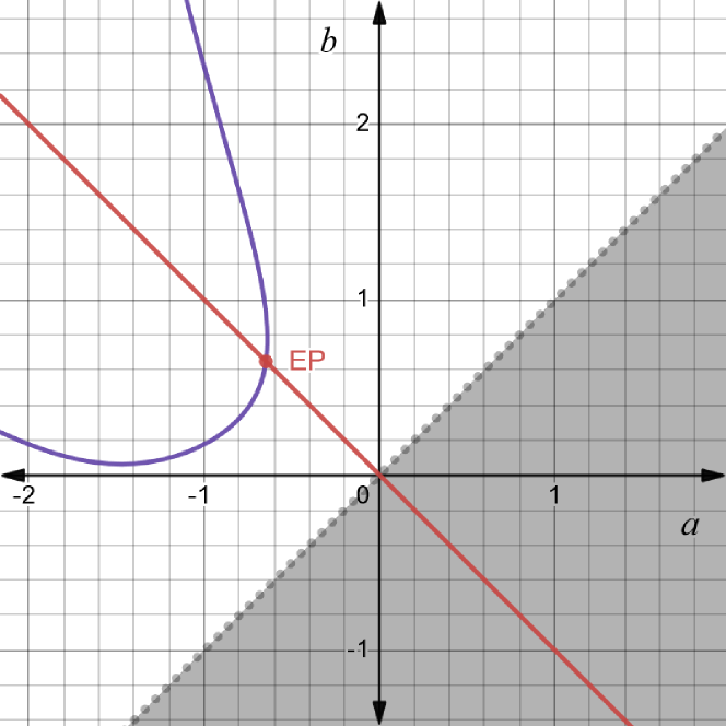
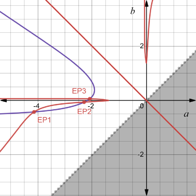
Figure 1: Mean reverting process (19) with constant volatility and multiplicative cost. On the left ($\theta=0.4,q_{d}=0.1,\lambda=1,s=2,\beta=1$) the equilibrium point (EP) is $(-0.646,0.646)$ with value $0.617$. On the right the assumption of Prop. 3.7 does not hold. The equilibrium points EP1 $\sim(-4.141,-0.421)$, EP2 $\sim(-2.297,-0.060)$, EP3 $\sim(-2.089,0.063)$ have respective values $1.391$, $0.1836$ and $0.000$

4.2 “Follow the market” examples

The idea is to introduce a cost function in such a way that the player has incentives to follow the market evolution. The cost function is then

$$c(x,y)=|x-y|.$$

4.2.1 Brownian motion with negative drift

In this case, the driving process is

$$X_{t}=\mu t+W_{t},$$

where $\{W_{t}\}_{t\geq 0}$ is a standard Brownian motion and $\mu<0$. The problem can be reduced to a one variable problem. The conclusions are:

• If there is a positive constant $C$ such that

  $$C(1+e^{2\mu C})(1-e^{2\mu C})^{-1}+(q_{d}+q_{u})\mu+\mu^{-1} =0,$$

  $$\Big{(}\frac{\displaystyle C}{\displaystyle e^{2\mu C}-1}\Big{)}\frac{\displaystyle 2e^{2\mu C}}{\displaystyle\mu}+\frac{\displaystyle-2e^{2\mu C}+2C\mu+1}{\displaystyle 2\mu^{2}}+q_{d}+q_{u} =0,$$

  then every point of the set $\{(a,a+C),a\in\mathbb{R}\}$ is an equilibrium point.

• Otherwise there are no equilibrium points.

The details can be found in the Appendix A.2.1

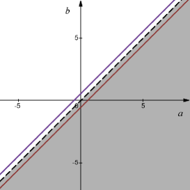
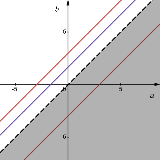
Figure 2: Brownian motion with drift and cost function $c(x,y)=|x-y|$. On the left ($q_{d}+q_{u}=0.1,\mu=-0.89$) the value at equilibrium points is constant $0.848$. On the right ($q_{d}+q_{u}=2,\mu=-1$ ) there are no equilibrium points

4.2.2 Ornstein Uhlenbeck process

In this case, the process $X_{t}$ follows the stochastic differential equation

$$dX_{t}=-\theta X_{t}dt+\sigma dW_{t},$$

We analyze the symmetric case when $q:=q_{d}=q_{u}$. The existence of equilibrium points will hold, but uniqueness not necessarily. Essentially, the equation $\pi_{1}(a,R(a,b))=\pi_{2}(a,R(a,b))$ is satisfied when $a=-b$ by symmetry, so similar arguments as the ones in the multiplicative case hold. However the line $a+b=0$ is not the only set where $\pi_{1}(a,R(a,b))=\pi_{2}(a,R(a,b))$ holds.

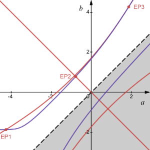
Figure 3: Mean reverting process with $q=0.1$, $\theta=3$, $s=2$, $EP1\sim(-4.26,-1.86)$, $EP2\sim(-0.78,0.78)$, $EP3\sim(1.87,4.27)$ with the values $0.839$, $0.55$ and $0.84$ at each equilibrium point respectively

5 Approximation of the symmetric $N$-player mean field game

5.1 Introduction and notations

In this section, we present an approximation result for ergodic mean-field games with $N$-players and the mean-filed game considered above, when the number of players $N$ tends to infinity. More precisely, we establish that an equilibrium point of the mean-field game defined in (3.3) is an $\epsilon$-Nash equilibrium of the corresponding $N$-player game (see Def. 5.1). These approximation results are now a classical issue in mean field games, and have been studied for instance in Haoyang et al. (2021) and Cao and Guo (2022) and the references therein.

In order to formulate our result we need the following notations.

• A filtered probability space $(\Omega,\mathcal{F},\{\mathcal{F}_{t}\},P)$ that satisfies the usual conditions, where all the processes are defined.

• Adapted independent Brownian motions $W,\{W^{i}\}_{i=1,2,\dots}$, with the corresponding processes $X,\{X^{i}\}_{i=1,2,\dots}$ each of one satisfy equation (1) driven by the respective $W$ or $W^{i}$.

• The set of admissible controls $\mathcal{A}$ of Definition 2.1, that in particular assumes, given an admissible control $(D^{i},U^{i})$, the existence of the controlled process as a solution of

  $$dX^{(D^{i},U^{i})}_{t}=\mu(X^{(D^{i},U^{i})}_{t})dt+\sigma(X^{(D^{i},U^{i})}_{t})dW_{t}-dD^{i}_{t}+dU^{i}_{t},\quad X_{0}=x,$$ (20)

  for each $i=1,2,\dots$

For simplicity and coherence we denote by $X^{i,(a,b)}$ the solution to (20) when the $i$-th player chooses reflecting strategies within $a<b$. As usual, we define the vector of admissible controls

$$\Lambda=((D^{1},U^{1}),\dots,(D^{N},U^{N}))$$

such that $(D^{i},U^{i})$ is an admissible control selected by the player $i$ in a game of $N$ players. Furthermore, we define

$$\Lambda^{-i}:=((D^{1},U^{1}),\dots,(D^{i-1},U^{i-1}),(D^{i+1},U^{i+1}),\dots,(D^{N},U^{N}))$$

and

$$V_{N}^{i}((D^{i},U^{i}),\Lambda^{-i})(x):=\\ \limsup_{T\rightarrow\infty}\frac{1}{T}\operatorname{\mathbf{E}}_{x}\Bigg{\{}\int_{0}^{T}c\bigg{[}X_{s}^{(D^{i},U^{i})},\frac{1}{N-1}\sum_{j\neq i}^{N}f(X_{s}^{(D^{j},U^{j})})\bigg{]}ds\\ +q_{u}dU^{i}_{s}+q_{d}dD^{i}_{s}\Bigg{\}}$$

for a cost function $c(x,y)$ satisfying Assumption 3.1 and a real function $f(x)$, that we assume continuous in this section.

Definition 5.1.

For a fixed $\epsilon>0$ and a fixed $N\in\mathbb{N},$ a vector of admissible controls $\Lambda=((D^{1},U^{1}),\dots,(D^{N},U^{N}))$ is called an $\epsilon$-Nash equilibrium if for every admissible control $\eta=(\overline{D}^{i},\overline{U}^{i})$:

$$V_{N}^{i}((D^{i},U^{i}),\Lambda^{-i})(x)\leq\epsilon+V_{N}(\eta,\Lambda^{-i})(x),\ \forall i=1,\dots,N,\ \forall x\in\mathbb{R}.$$

5.2 Approximation to the ergodic mean-field problem

We are ready to prove that the equilibrium points of the mean-field game are $\epsilon$-equilibrium points for the $N$-player game. It is interesting to notice that the proofs are quite simple due to the fact that the controlled process is bounded.

Theorem 5.2.

Assume that there is a convex increasing function $F\colon\mathbb{R}\rightarrow\mathbb{R}_{+}$ and a continuous function $g\colon\mathbb{R}\rightarrow\mathbb{R}_{+}$ such that the cost function $c(x,y)$ satisfies

$$|c(x,y_{1})-c(x,y_{2})|\leq F(|x|)|g(y_{1})-g(y_{2})|.$$ (21)

Suppose that the point $(D^{b},U^{a})$ is an equilibrium for the problem defined in (3.3) and there is a set $\mathcal{C}\subset\mathcal{A}$ such that the control $(D^{b},U^{a})\in\mathcal{C}$ and the following two conditions hold:

$$\sup_{\eta\in\mathcal{C}}\limsup_{T\rightarrow\infty}\frac{1}{T}\operatorname{\mathbf{E}}_{x}\left(\int_{0}^{T}F(X_{s}^{\eta})ds\right)<\infty\ \forall x\in\mathbb{R},$$ (22)

$$\inf_{\eta\in\mathcal{B}}V_{N}^{i}(\eta,\Lambda^{-i})(x)=\inf_{\eta\in\mathcal{C}}V_{N}^{i}(\eta,\Lambda^{-i})(x),\ \forall N\in\mathbb{N},\ x\in\mathbb{R},$$

where

$$\Lambda:=((D^{b},U^{a}),(D^{b},U^{a})\dots,(D^{b},U^{a})).$$

Then, the vector of controls $\Lambda$ is an $\epsilon_{N}$-Nash equilibrium for the $N$-player game, with $\epsilon_{N}\rightarrow 0$ when $N\rightarrow\infty$.

Remark 5.3.

Note that for the values of the parameters $\lambda>0$, $\beta>0$ and $\alpha\geq 1$, the cost functions

$$(x,y)\rightarrow\{-\lambda x,x\}^{\alpha}(1+|y|^{\beta}),\quad(x,y)\rightarrow|\beta x-y|$$

satisfy condition (21) (see Appendix A.1).

Proof.

First of all define the function

$$V\colon\mathcal{C}\times\{(a,b);a<b\}\times\mathbb{R}\rightarrow\mathbb{R}$$

via

$$V((D,U),(b,a))(x)=\\ \limsup_{T\rightarrow\infty}\frac{1}{T}\operatorname{\mathbf{E}}_{x}\left[\int_{0}^{T}c\big{(}X_{s}^{D,U},\operatorname{\mathbf{E}}_{x}(f(X^{a,b}_{s}))\big{)}ds+q_{u}dU_{T}+q_{d}dD_{T}\right].$$

From now on, as $x$ is fixed along the proof, we omit it. We only need to work with controls in the set $\mathcal{C}$. For a fixed $N$ define

$$\Lambda:=((D^{b},U^{a}),(D^{b},U^{a}),\dots,(D^{b},U^{a})),$$

consider $\eta\in\mathcal{C}$ and observe that

$$V_{N}^{i}(\Lambda) =V_{N}^{i}(\eta,\Lambda^{-i})+\big{(}V_{N}^{i}(\Lambda)-V(\eta,(b,a))\big{)}+\big{(}V(\eta,(b,a))-V_{N}^{i}(\eta,\Lambda^{-i})\big{)}$$

$$\leq V_{N}^{i}(\eta,\Lambda^{-i})+\big{(}V_{N}^{i}(\Lambda)-V((D^{b},U^{a}),(b,a))\big{)}+\big{(}V(\eta,(b,a))-V_{N}^{i}(\eta,\Lambda^{-i})\big{)}.$$

Therefore it is enough to prove that

$$\sup_{\eta\in\mathcal{C}}|V_{N}^{i}(\eta,\Lambda^{-i})-V(\eta,(b,a))|\rightarrow 0,$$ (23)

when $N\rightarrow\infty$, as the other term $|V_{N}^{i}(\Lambda)-V((D^{b},U^{a}),(b,a))|$ is a particular case of (23) when $\eta=(D^{b},U^{a})$. We proceed to prove (23):

$$\limsup_{T\rightarrow\infty}\frac{1}{T}\operatorname{\mathbf{E}}_{x}\left\{\int_{0}^{T}\left[c\left(X_{s}^{\eta},\bigg{(}\frac{1}{N-1}\sum_{j\neq i}^{N}f(X_{s}^{j,(a,b)})\bigg{)}\right)-c\Big{(}X_{s}^{\eta},\operatorname{\mathbf{E}}_{x}\big{(}f(X_{s}^{a,b}))\Big{)}\right]ds\right\}$$

$$\leq\limsup_{T\rightarrow\infty}\operatorname{\mathbf{E}}_{x}\left\{\int_{0}^{T}\Bigg{[}\frac{1}{T}F(X_{s}^{i,\eta})\Bigg{|}g\Big{(}\operatorname{\mathbf{E}}_{x}\big{(}f(X_{s}^{a,b})\big{)}\Big{)}-g\bigg{(}\frac{1}{N-1}\sum_{j\neq i}^{N}f(X_{s}^{j,(a,b)})\bigg{)}\Bigg{|}\Bigg{]}ds\right\}$$

$$=\limsup_{T\rightarrow\infty}\int_{0}^{T}\Bigg{\{}\frac{1}{T}\operatorname{\mathbf{E}}_{x}\Bigg{[}F(X_{s}^{i,\eta})\Bigg{|}g\left(\operatorname{\mathbf{E}}_{x}\big{(}f(X_{s}^{a,b})\big{)}\right)-g\bigg{(}\frac{1}{N-1}\sum_{j\neq i}^{N}f(X_{s}^{j,(a,b)})\bigg{)}\Bigg{|}\Bigg{]}ds\Bigg{\}}.$$ (24)

Define $K:=\max_{x\in[a,b]}g(x)$ and $M:=\sup_{s\in\mathbb{R}^{+},x\in\mathbb{R}}\left\{\sqrt{\text{var}_{x}(f\big{(}X_{s}^{(a,b)})\big{)}}\right\}$ ($\mathrm{var}_{x}$ is the variance of the process started at $x$), let $\epsilon>0$ be arbitrary, $\delta>0$ such that $|g(y_{1})-g(y_{2})|<\epsilon$ if $|y_{1}-y_{2}|<\delta M$ for all $y_{1},y_{2}\in[a,b$] and $N\in\mathbb{N}$. Invoking Chebyshev’s inequality:

$$P\Bigg{(}\bigg{|}\operatorname{\mathbf{E}}_{x}(f\big{(}X_{s}^{a,b})\big{)}-\frac{1}{N-1}\sum_{j\neq i}^{N}f(X_{s}^{j,(a,b)})\bigg{|}\geq M\delta\Bigg{)}\leq\frac{1}{\delta^{2}(N-1)}.$$

Therefore the term (5.2) is smaller or equal than

$$\limsup_{T\rightarrow\infty}\left(\frac{K}{\delta^{2}(N-1)}+\epsilon\right)\left(\int_{0}^{T}\frac{1}{T}\operatorname{\mathbf{E}}_{x}(F(X_{s}^{i,\eta}))ds\right).$$

The integral is uniformly bounded by assumption (22), concluding that the limit is zero because $\epsilon$ is arbitrary. ∎

Statements and Declarations

The second and third authors are supported by CSIC - Proyecto grupos nr. 22620220100043UD, Universidad de la República, Uruguay.

Appendix A Appendix

A.1 Approximation for the cost in examples

First of all notice that

$$\big{|}\ |x-y_{1}|-|x-y_{2}|\ \big{|}\leq|y_{1}-y_{2}|$$

Therefore for the cost $(x,y)\rightarrow|x-y|$ we take $F\equiv 1$ and conclude that the function is trivially on the hypothesis of Theorem 5.2.
For the multiplicative case suppose there is an equilibrium at $(a,b)$ for the mean-field game for a cost function $c(x,y)=f(x)g(y)$ with both $f,g$ non negative, continuous, convex with minimum at zero with $g(0)=1$. We take $F\equiv f$.
Consider $\Lambda$ as in (5.2) (it depends on $N$) and assume there is a sequence $\{N_{K}\}\subset\mathbb{N}$ and a sequence $\{\epsilon_{K}\},\ \epsilon_{K}\rightarrow 0,$ when $K\rightarrow\infty$ such that if a control $\eta_{K}\in\mathcal{B}$ satisfies

$$\inf_{\eta\in\mathcal{B}}V_{N_{K}}^{i}(\eta,\Lambda^{-i})+\epsilon_{K}>V_{N_{K}}^{i}(\eta_{K},\Lambda^{-i})$$

then

$$\limsup_{T\rightarrow\infty}\frac{1}{T}\operatorname{\mathbf{E}}_{x}\left(\int_{0}^{T}f(X_{s}^{\eta,i})ds\right)>K.$$

With that control we get

$$V_{N_{K}}^{i}(\eta_{r},\Lambda^{-i})=\\ \limsup_{T\rightarrow\infty}\frac{1}{T}\operatorname{\mathbf{E}}_{x}\left(\int_{0}^{T}f(X_{s}^{\eta_{K}})g\bigg{(}\frac{1}{N-1}\sum_{j\neq i}^{N}X_{s}^{i,(a,b)}\bigg{)}+\eta_{1,K}(s)q_{d}+\eta_{2,K}(s)q_{u}ds\right)\\ >K_{r}.\hskip 14.22636pt$$ (25)

Therefore the set

$$\bigg{\{}\inf_{\eta\in\mathcal{B}}V_{N}^{i}(\eta,\Lambda^{-i}),\ N\in\mathbb{N}\bigg{\}}$$

is not bounded above. This is absurd because $g$ restricted in $[a,b]$ is bounded and is the only term that depends on $N$.

A.2 Calculations of the examples

A.2.1 Absolute value, Brownian motion with negative drift

In this case (see Borodin and Salminen (2002)),

$$S^{\prime}(x)=\exp(-2\mu x),\ m^{\prime}(x)=2e^{2\mu x}.$$

Therefore

$$R(a,b) =\frac{\displaystyle\int_{a}^{b}2ue^{2\mu u}du}{\displaystyle\int_{a}^{b}2e^{2\mu u}du}=\frac{\displaystyle be^{2\mu b}-ae^{2\mu a}}{\displaystyle e^{2\mu b}-e^{2\mu a}}-\frac{1}{2\mu}.$$

The cost function is $c(x,y)=|x-y|.$ We proceed to analyze the function $\rho$. The notations are the same as Proposition 3.7.

The equation $\pi_{2}(a,R(a,b))=\pi_{1}(b,R(a,b))$ is equivalent to

$$F(a,b)=(b+a)+\frac{1}{\mu}-2\left(\frac{\displaystyle be^{2\mu b}-ae^{2\mu a}}{e^{2\mu b}-e^{2\mu a}}\right)+\mu(q_{u}+q_{d})=0.$$

On one hand, when $a<0$ the equation $F(a,b)=0$ has a solution $b>0$ because

$$a+\mu^{-1}+\mu(q_{d}+q_{u})<0$$

On the other hand when $a\geq 0,$ the equation $F(a,b)=0$ also has a root because $b-2R(a,b)\to-\infty$ when $b\to\infty$.
We compute the partial derivative

$$\frac{\partial F}{\partial b}(a,b)=-1\frac{\displaystyle(e^{2\mu(b-a)})\left(2\mu(a-b)-1+e^{2\mu(b-a)}\right)}{\displaystyle(1-e^{2\mu(b-a)})^{2}}>0.$$

We deduce that the function $\rho$ is well defined in all $\mathbb{R}$ and the roots of $F(a,b)$ are unique for each $a$. Furthermore if $C$ is the positive constant that satisfies the equality

$$C(1+e^{2\mu C})(1-e^{2\mu C})^{-1}=-(q_{d}+q_{u})\mu-\mu^{-1},$$

then $F(a,a+C)=0$. So $\rho(a)=a+C$.

From Theorem 3.5 we know the equilibrium points $(a,b)$ must satisfy the equality:

$$\int_{a}^{b}(|t-R(a,b)|-b+R(a,b))2e^{2\mu t}dt+(q_{d}+q_{u})e^{2\mu a}=0.$$ (26)

More explicity:

$$\int_{a}^{b}\bigg{(}\Big{|}t+\frac{1}{2\mu}-\frac{\displaystyle be^{2\mu b}-ae^{2\mu a}}{\displaystyle e^{2\mu b}-e^{2\mu a}}\Big{|}-b-\frac{1}{2\mu}+ \frac{\displaystyle be^{2\mu b}-ae^{2\mu a}}{\displaystyle e^{2\mu b}-e^{2\mu a}}\bigg{)}2e^{2\mu t}dt$$

$$+(q_{d}+q_{u})e^{2\mu a}=0$$ (27)

With the change of variable $u=t-b$ the equality (A.2.1) is equivalent to:

$$\int_{a-b}^{0}\bigg{(}\Big{|}u-\frac{\displaystyle(b-a)}{\displaystyle e^{2\mu(b-a)}-1}+\frac{1}{2\mu}\Big{|}+\frac{\displaystyle(b-a)}{\displaystyle e^{2\mu(b-a)}-1}-\frac{1}{2\mu}\bigg{)} 2e^{2\mu(u+b-a)}du\ e^{2\mu a}$$

$$+(q_{d}+q_{u})e^{2\mu a}=0.$$ (28)

Therefore if there is a point $(A,B)$ that satisfies (A.2.1) then every point $(a,b)$ such that $b-a=B-A$ also satisfies (A.2.1). To solve the integral define $C\coloneqq b-a$ and $K\coloneqq C(\exp(2\mu C)-1)^{-1}-(2\mu)^{-1}$ so the integral in (A.2.1) becomes

$$\int_{-C}^{0} \bigg{(}\Big{|}u-K\Big{|}+K\bigg{)}2e^{2\mu(C+u)}du=$$

$$2e^{2\mu K}\int_{-C-K}^{-K}|r|e^{2\mu(C+r)}dr+Ke^{2\mu C}\frac{1-e^{-2\mu C}}{\mu}=$$

$$\frac{2}{4\mu^{2}}e^{2\mu(K+C)}\bigg{(}e^{2\mu r}(2\mu r-1)\big{|}^{0}_{-C-K}-e^{2\mu r}(2\mu r-1)\big{|}^{-K}_{0}\bigg{)}$$

$$+Ke^{2\mu C}\frac{1-e^{-2\mu C}}{\mu}=$$

$$\frac{1}{2\mu^{2}}e^{2\mu C}(-e^{-2\mu C}(2\mu(-C-K)-1)-(-2\mu K-1))$$

$$+Ke^{2\mu C}\frac{1-e^{-2\mu C}}{\mu}=$$

$$e^{2\mu C}\Bigg{(}\frac{\displaystyle 4\mu K+1}{\displaystyle 2\mu^{2}}\bigg{)}+\frac{2C\mu+1}{2\mu^{2}}=$$

$$\Big{(}\frac{\displaystyle C}{\displaystyle e^{2\mu C}-1}\Big{)}\frac{\displaystyle 2e^{2\mu C}}{\displaystyle\mu}+\frac{\displaystyle-2e^{2\mu C}+2C\mu+1}{\displaystyle 2\mu^{2}}.$$

Solving the integral in (A.2.1) we conclude that a point $(a,b)$ is an equilibrium point iff $C\coloneqq b-a$ satisfies

$$C(1+e^{2\mu C})(1-e^{2\mu C})^{-1}+(q_{d}+q_{u})\mu+\mu^{-1}=0$$

$$\Big{(}\frac{\displaystyle C}{\displaystyle e^{2\mu C}-1}\Big{)}\frac{\displaystyle 2e^{2\mu C}}{\displaystyle\mu}+\frac{\displaystyle-2e^{2\mu C}+2C\mu+1}{\displaystyle 2\mu^{2}}+q_{d}+q_{u}=0$$

Using 3.4 it can be shown that the value is be the same for all equilibrium points and it is

$$-C\exp(-2\mu C)(1-\exp(-2\mu C))^{-1}-(2\mu)^{-1}+q_{d}\mu$$

A.2.2 Multiplicative cost

Proposition 3.7 is used with $A=0$. We assume $\lambda\geq 1$ (in other cases symmetrical arguments can be used), $c(x,y)=\max(-\lambda x,x)(1+|y|^{\beta})$, $q:=q_{d}=q_{u}\lambda^{-1},\ \beta>0$ and $q_{d}\theta<1\wedge\lambda^{-1}$ so the function $c$ is a cost function.

The equality $\pi_{1}(b,R(a,b))=\pi_{2}(a,R(a,b))$ reads as $-\lambda a=b$ . Furthermore if $\sigma$ is an even function we deduce $R(a,-\lambda a)$ is decreasing in $a$ so:

$$\pi_{2}(t,L(a))-\pi_{2}(a,L(a))=(a-t)(1+R(a,-\lambda a)^{\beta}-q_{d}\lambda\theta)$$

which decreases to $-\infty$ in $a$.

$$\pi_{1}(t,L(a))-\pi_{1}(-\lambda a,L(a))=(t-\lambda a)(1+R(a,-\lambda a)^{\beta}-q_{u}\theta)$$

which decrease to $-\infty$ implying that uniqueness and existence holds.
In the case $1\wedge\lambda^{-1}\geq\theta q_{d}$ the function $c(x,y)$ is not a cost function so existence and uniqueness is not guaranteed.

References

• Alvarez (2018) Alvarez, L.H.R.: A Class of Solvable Stationary Singular Stochastic Control Problems. https://doi.org/10.48550/arXiv.1803.03464 (2018)
• Alvarez and Shepp (1998) Alvarez, L. H. R., Shepp, L. A.: Optimal harvesting of stochastically fluctuating populations. Journal of Mathematical Biology 37, 155–177 (1998)
• Asmussen and Taksar (1997) Asmussen, S., Taksar, M.: Controlled diffusion models for optimal dividend pay-out. Insurance: Mathematics and Economics 20, 1–15 (1998)
• Borodin and Salminen (2002) Borodin, A., Salminen, P.: Handbook on Brownian motion - facts and formulae, 2nd ed. (2nd printing). Birkhäuser, Basel (2002)
• Haoyang et al. (2021) Cao, H., Dianetti, J., Ferrari, G.: Stationary Discounted and Ergodic Mean Field Games of Singular Control. https://doi.org/10.48550/arXiv.2105.07213 (2021)
• Cao and Guo (2022) Cao, H., Guo, X.: MFGs for partially reversible investment. Stochastic Processes and their Applications 150, 995–1014 (2002)
• Carmona (2020) Carmona, R.: Applications of Mean Field Games in Financial Engineering and Economic Theory. https://doi.org/10.48550/arXiv.2012.05237 (2020)
• Festa and Göttlich (2018) Festa, A., Göttlich, S.: A Mean Field Game approach for multi-lane traffic management. IFAC-PapersOnLine 51(32), 793–798 (2018)
• Hening, Nguyen, Ungureanu and Wong (2017) Hening, A., Nguyen, D. H., Ungureanu, S. C., and Wong, T. K.: Asymptotic harvesting of populations in random environments. https://doi.org/10.48550/arXiv.1710.01221 (2017)
• H$\o$jgaard and Taksar (2001) H$\o$jgaard, B., Taksar, M.: Optimal risk control for a large corporation in the presence of returns on investments. Finance and Stochastics 5, 527–547 (2001)
• Huang (2013) Huang, M.: A Mean Field Capital Accumulation Game with HARA Utility. Dynamic Games and Applications 3, 446–472 (2013)
• Huang et al. (2004) Huang, M., Caines, P. E., Malhame, R. P.: Large-population cost-coupled LQG problems: generalizations to non-uniform individuals. 2004 43rd IEEE Conference on Decision and Control, 3453–3458 (2004)
• Jeanblanc-Picqué and Shiryaev (1995) Jeanblanc-Picqué, M. and Shiryaev, A. N.: Optimization of the flow of dividends. Russian Math. Surveys 50, 257–277 (1995)
• Kunwai et al. (2022) Kunwai, K., Xi, F., Yin, G., Zhu, C.: On an Ergodic Two-Sided Singular Control Problem. Applied Mathematics and Optimization 86, 26 (2022)
• Lande and Engen and Sæther (1994) Lande, R., Engen S., Sæther B. E.: Optimal harvesting, economic discounting and extinction risk in fluctuating populations. Nature, 372, 88–90 (1994)
• Paulsen (2008) Paulsen, J.: Optimal dividend payments and reinvestments of diffusion processes with fixed and proportional costs. SIAM Journal on Control and Optimization 47, 2201–2226 (2008)
• Peura and Keppo (2006) Peura, S., Keppo, J. S.: Optimal Bank Capital with Costly Recapitalization. Journal of Business 79, 2163–2201 (2006)
• Protter (2005) Protter, P. E.: Stochastic integration and differential equations, 2nd. edition. Springer, Berlin Heildeberg (2005)
• Rogers and Williams (2000) Rogers, L.C.G., Williams, D.: Diffusions, Markov processes and Martingales, Volume 2: It$\hat{\text{o}}$ Calculus, 2nd edition. Cambridge University Press, Cambridge (2000)
• Saisho (1987) Saisho, Y.: Stochastic differential equations for multidimensional domain with reflecting boundary. Probab. Theory Related Fields 74 (1987), no. 3.
• Shreve et al. (1984) Shreve, S., Lehoczky, J., Gaver, D.: Optimal consumption for general diffusion with absorbing and reflecting barriers. SIAM Journal on Control and Optimization 22, 55–75 (1984)