Fast multi-channel inverse design through augmented partial factorization

Abstract

Computer-automated design and discovery have led to high-performance nanophotonic devices with diverse functionalities. However, massively multi-channel systems such as metasurfaces controlling many incident angles and photonic-circuit components coupling many waveguide modes still present a challenge. Conventional methods require $M_{\rm in}$ forward simulations and $M_{\rm in}$ adjoint simulations—$2M_{\rm in}$ simulations in total—to compute the objective function and its gradient for a design involving the response to $M_{\rm in}$ input channels. By generalizing the adjoint method and the recently proposed augmented partial factorization method, here we show how to obtain both the objective function and its gradient for a massively multi-channel system in a single simulation, achieving over-two-orders-of-magnitude speedup and reduced memory usage. We use this method to inverse design a metasurface beam splitter that separates the incident light to the target diffraction orders for all incident angles of interest, a key component of the dot projector for 3D sensing. This formalism enables efficient inverse design for a wide range of multi-channel optical systems.

I Introduction

Nanoengineered photonic devices can realize versatile and high-performance functionalities in a compact footprint, expanding the limited scope of conventional optical components. Computer-automated inverse design [1, 2, 3, 4, 5, 6, 7] can search a high-dimensional parameter space to discover optimal structures that outperform manual designs or realize new functionalities. With inverse design, the photonic structure is updated iteratively to optimize an objective function $f$ that encapsulates the desired properties. Given the many parameters ${\bf p}=\{p_{k}\}$ used to parametrize the design, efficient optimization typically requires the gradient $\bm{\nabla}_{\bf p}f$ of the objective function with respect to all parameters. The computational efficiency is a critical consideration since full-wave simulations are necessary to model the complex light-matter interactions at the subwavelength scale, and numerous simulations are needed for the many iterations of the search process.

When the objective function $f$ involves the response to just one input (e.g., one incident angle) or one output (e.g., one outgoing angle), the adjoint method can compute the complete gradient $\bm{\nabla}_{\bf p}f$ using only one forward and one adjoint simulations [3, 4, 5]. However, when $f$ involves $M_{\rm in}\gg 1$ inputs, the adjoint method requires $2M_{\rm in}$ simulations ($M_{\rm in}$ forward, $M_{\rm in}$ adjoint) [8]. This prohibits the inverse design of large multi-channel systems. There are many such multi-channel systems including photonic circuits [9] and aperiodic meta-structures for applications in wide-field-of-view metalenses [8, 10, 11, 12], beam combiners [13, 14], angle-multiplexed holograms [15, 16], concentrators [10, 17], thermal emission control [18, 19, 20], image processing [21, 22, 23, 24, 25, 26, 27], optical computing [28, 29], space compression [30, 31, 32], etc. The inverse design of these systems remains challenging.

We recently proposed the “augmented partial factorization” (APF) method, which can solve multi-input electromagnetic forward problems in one shot, offering substantial speed-up and memory usage reduction compared to existing methods [33]. But the inverse problem was unsolved since the formalism of Ref. [33] does not yield the gradient. Here, we generalize APF to enable efficient gradient computation for multi-input problems. We are able to obtain both $f$ and $\bm{\nabla}_{\bf p}f$ in a single or a few computations without a loop over the individual input channels. For a 1-mm-wide metasurface with 2400 inputs, APF achieves $\sim$150 times speed-up and $\sim$30% memory usage reduction compared to the conventional adjoint method. As an example problem, we inverse design a metasurface beam splitter that splits the incident light equally into the $\pm$1 diffraction orders over an incident angular range of 60^∘.

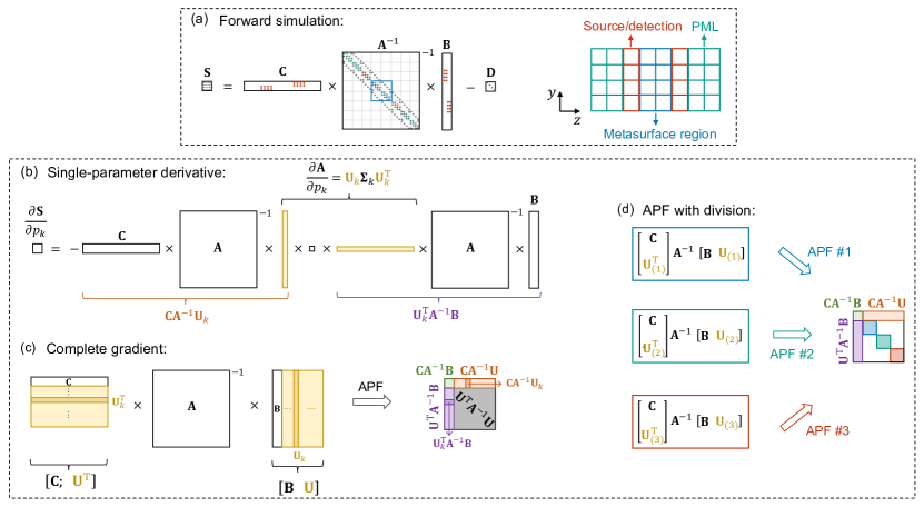
Figure 1: Schematics of using augmented partial factorization (APF) for (a) forward simulation and (b–d) gradient computation. (a) Illustration of $\mathbf{S=CA}^{-1}\mathbf{B-D}$, where the multi-channel response is encapsulated in a generalized scattering matrix $\mathbf{S}$ given in terms of the discretized Maxwell operator matrix $\bf A$, the source profiles $\bf B$, the projection profiles $\bf C$, and the baseline $\bf D$ from the incident field. Dots represent nonzero elements of these sparse matrices, with colors corresponding to different regions of the simulation domain. PML: perfectly matched layer. (b) Illustration of Eqs. (2–3) for a single derivative: after decomposing $\partial\mathbf{A}/\partial p_{k}$ into $\mathbf{U}_{k}{\bm{\Sigma}}_{k}\mathbf{U}_{k}^{\rm T}$ and regrouping the terms, $\mathbf{CA}^{-1}\mathbf{U}_{k}$ and $\mathbf{U}_{k}^{\rm T}\mathbf{A}^{-1}\mathbf{B}$ can be computed to yield $\partial\mathbf{S}/\partial p_{k}$. (c) Illustration of Eq. (4) for the full gradient: by combining $\mathbf{U}_{k}$ for all parameters $\{p_{k}\}$ and augmenting them to $\mathbf{B}$ and $\mathbf{C}$, a single APF computation can yield the complete gradient with respect to all parameters. (d) By dividing $\mathbf{U}$ and performing $N_{\rm sub}$ separate APF computations ($N_{\rm sub}=3$ in this illustration), we can obtain the same $\mathbf{CA}^{-1}\mathbf{B}$, $\mathbf{CA}^{-1}\mathbf{U}$, and $\mathbf{U}^{\rm T}\mathbf{A}^{-1}\mathbf{B}$ with less computing time and memory by evaluating only $1/N_{\rm sub}$ of the unnecessary matrix $\mathbf{U^{\rm T}A}^{-1}\mathbf{U}$ and by storing smaller matrices $\mathbf{CA}^{-1}\mathbf{U}_{(n)}$ and $\mathbf{U}^{\rm T}_{(n)}\mathbf{A}^{-1}\mathbf{B}$ in memory.

II Multi-input gradient computation using APF

The novelty of the APF method lies in encapsulating the linear response of the multi-channel system in a generalized scattering matrix $\mathbf{S=CA}^{-1}\mathbf{B-D}$ and then computing the entire $\mathbf{S}$ in a single shot through the partial factorization of an augmented matrix ${\bf{K}}=\left[{{\bf{A}},{\bf{B}};{\bf{C}},{\bf{D}}}\right]$ that yields its Schur complement $-\mathbf{CA}^{-1}\mathbf{B}$ [33]. Here, the $S_{nm}$ element of the $M_{\rm out}\times M_{\rm in}$ matrix $\mathbf{S}$ is the field amplitude in output channel $n$ given an input in channel $m$ at frequency $\omega$. Matrix $\mathbf{A}$ is the discretized Maxwell differential operator $-(\omega/c)^{2}\varepsilon_{\rm{r}}({\bf{r}})+\nabla\times\nabla\times$ of the structure defined by its relative permittivity profile $\varepsilon_{\rm{r}}({\bf{r}})$, the $M_{\rm in}$ columns of matrix $\mathbf{B}$ contain the $M_{\rm in}$ distinct input source profiles, the $M_{\rm out}$ rows of matrix $\mathbf{C}$ contain the $M_{\rm out}$ output projection profiles, and matrix $\mathbf{D}$ subtracts the baseline contribution from the incident field; they are schematically shown in Fig. 1a. If the number of nonzero elements in matrices $\mathbf{B}$, $\mathbf{C}$, and $\mathbf{S}$ are less than the number of nonzero elements in matrix $\mathbf{A}$, the single-shot computing time and memory usage of APF will be independent of how many input and output channels there are [33]. In the following, we use APF with finite-difference discretization implemented in our open-source software MESTI [34], using the MUMPS package for factorization [35].

Here, we derive a general formulation such that the gradient of any multi-channel objective function can also be computed in a single shot regardless of the number $M_{\rm in}$ of input channels. We use vector $\mathbf{p}=[p_{1},\cdots,p_{N_{p}}]$ to denote the $N_{p}$ real-valued variables parameterizing the photonic design; in the example later, $\{p_{k}\}$ will be the edge positions of the ridges of a metasurface. The objective function $f$ (also called the figure of merit, FoM) that evaluates the performance of the multi-channel device is a function of the generalized scattering matrix $\mathbf{S}$ and the parameters $\mathbf{p}$, namely $f[\mathbf{S}(\mathbf{p}),\mathbf{p}]$. The gradient $df/dp_{k}$ we want follows from the chain rule as

$$\frac{df}{dp_{k}}=\frac{\partial f}{\partial p_{k}}+\sum_{n=1}^{M_{\rm out}}\sum_{m=1}^{M_{\rm in}}2{\rm Re}\left(\frac{\partial f}{\partial S_{nm}}\frac{\partial S_{nm}}{\partial p_{k}}\right).$$ (1)

Note that $S_{nm}$ is complex-valued, and $\partial f/\partial S_{nm}$ is a Wirtinger derivative. Both $\partial f/\partial p_{k}$ and $\partial f/\partial S_{nm}$ can be calculated analytically given the definition of the objective function $f$ for a specific problem. So, the simulations only need to evaluate the derivative of the scattering matrix, $\partial S_{nm}/\partial p_{k}$.

The parameters $\{p_{k}\}$ modify the scattering matrix $\mathbf{S}$ by modifying the photonic structure $\varepsilon_{\rm{r}}({\bf{r}})$ in the Maxwell operator $\mathbf{A}$. Taking the derivative of $\mathbf{S=CA}^{-1}\mathbf{B-D}$ and using the identity $\partial{\bf A}^{-1}/\partial p_{k}=-{\bf A}^{-1}(\partial{\bf A}/\partial p_{k}){\bf A}^{-1}$, we get $\partial\mathbf{S}/\partial p_{k}=-\mathbf{CA}^{-1}(\partial\mathbf{A}/\partial p_{k})\mathbf{A}^{-1}\mathbf{B}$. Here we assume that matrices $\mathbf{B}$, $\mathbf{C}$, and $\mathbf{D}$ do not depend on $\{p_{k}\}$; additional terms can be added if there is such dependence. This generalizes the adjoint method to multi-channel systems: the columns of $\mathbf{A}^{-1}\mathbf{B}$ correspond to $M_{\rm in}$ forward problems, and the rows of $\mathbf{CA}^{-1}$ correspond to $M_{\rm out}$ adjoint problems. To recover the conventional adjoint method, one can substitute $\partial\mathbf{S}/\partial p_{k}$ into Eq. (1) and sum over the output channels for each input, which converts the $M_{\rm out}$ adjoint problems to $M_{\rm in}$ adjoint problems.

A key observation is that the derivative $\partial\mathbf{A}/\partial p_{k}$ above is a low-rank matrix since only a few elements of $\mathbf{A}$ depend on the parameter $p_{k}$. For example, with 2D transverse magnetic (TM) waves at angular frequency $\omega$, matrix $\mathbf{A}$ is the discretized version of $-{\nabla^{2}}-\left(\omega/c\right)^{2}{\varepsilon_{\rm{r}}}\left({\bf{r}}\right)$, and $\partial\mathbf{A}/\partial p_{k}$ is zero everywhere except for the few diagonal elements corresponding to pixels where the relative permittivity profile $\varepsilon_{\rm{r}}(\bf r)$ is modified by $p_{k}$. Matrix $\partial\mathbf{A}/\partial p_{k}$ is also symmetric due to reciprocity. Therefore, we can do a symmetric singular value decomposition

$$\partial\mathbf{A}/\partial p_{k}=\mathbf{U}_{k}\bm{\Sigma}_{k}\mathbf{U}_{k}^{\rm T},$$ (2)

where $\bm{\Sigma}_{k}$ is an $r_{k}$-by-$r_{k}$ diagonal matrix containing the singular values, $r_{k}$ is the rank of $\partial\mathbf{A}/\partial p_{k}$, the $r_{k}$ columns of $\mathbf{U}_{k}$ are the left-singular vectors (which are real-valued and equal the right-singular vectors), and ^T stands for matrix transpose. These singular vectors are zero everywhere except at the pixels where $\varepsilon_{\rm{r}}(\bf r)$ is modified by $p_{k}$.

We then obtain the derivative of the scattering matrix with respect to the $k$-th parameter

$$\partial\mathbf{S}/\partial p_{k}=-(\mathbf{CA}^{-1}\mathbf{U}_{k})\bm{\Sigma}_{k}(\mathbf{U}_{k}^{\rm T}\mathbf{A}^{-1}\mathbf{B}),$$ (3)

as shown in Fig. 1b. To obtain the complete gradient with respect to all $N_{p}$ parameters $\{p_{k}\}$, we combine the singular-vector matrices as $\mathbf{U}\equiv[\mathbf{U}_{1},\cdots,\mathbf{U}_{N_{p}}]$, which has $M_{p}\equiv\sum_{k=1}^{N_{p}}r_{k}$ columns. Computing $\mathbf{CA}^{-1}\mathbf{U}=[\mathbf{CA}^{-1}\mathbf{U}_{1},\cdots,\mathbf{CA}^{-1}\mathbf{U}_{N_{p}}]$ and $\mathbf{U}^{\rm T}\mathbf{A}^{-1}\mathbf{B}=[\mathbf{U}_{1}^{\rm T}\mathbf{A}^{-1}\mathbf{B};\cdots;\mathbf{U}_{N_{p}}^{\rm T}\mathbf{A}^{-1}\mathbf{B}]$ with APF would yield the complete gradient through Eqs. (1–3) with just two APF computations. As shown in Fig. 1c, we can further reduce from two APF computations to one by building new matrices $\mathbf{\tilde{B}=[B,U]}$ and $\mathbf{\tilde{C}=[C;U^{\rm T}]}$ and using APF to compute

$$\mathbf{\tilde{S}}=\mathbf{\tilde{C}A}^{-1}\mathbf{\tilde{B}}=\begin{aligned} \left[\begin{matrix}\mathbf{C}\\ \mathbf{U^{\rm T}}\end{matrix}\right]\mathbf{A}^{-1}\left[\begin{matrix}\mathbf{B}&\mathbf{U}\end{matrix}\right]=\left[\begin{matrix}\mathbf{CA}^{-1}\mathbf{B}&\mathbf{CA}^{-1}\mathbf{U}\\ \mathbf{U^{\rm T}A}^{-1}\mathbf{B}&\mathbf{U^{\rm T}A}^{-1}\mathbf{U}\end{matrix}\right]\end{aligned}$$ (4)

Here, the matrix $\mathbf{\tilde{K}}=\left[{{\bf{A}},\mathbf{\tilde{B}};\mathbf{\tilde{C}},{\bf{0}}}\right]$ is augmented with not only the original $M_{\rm in}$ input and $M_{\rm out}$ output channel profiles $\mathbf{B}$ and $\mathbf{C}$ but also $M_{p}$ additional inputs/outputs being the singular vectors $\mathbf{U}$ and $\mathbf{U}^{\rm T}$ from the design parameters $\{p_{k}\}$. This way, a single-shot APF computation solves all of the $M_{\rm in}$ forward simulations (yielding the scattering matrix ${\bf S}$ from $\mathbf{CA}^{-1}\mathbf{B}$) and also obtains the complete gradient (i.e., $\partial\mathbf{S}/\partial p_{k}$ and $df/dp_{k}$ for all $p_{k}$, from $\mathbf{CA}^{-1}\mathbf{U}$ and $\mathbf{U^{\rm T}A}^{-1}\mathbf{B}$) at the same time.

While a single APF computation suffices, doing so is not necessarily the most computationally efficient. When the number of elements in matrix $\mathbf{\tilde{S}}$, $\mathrm{numel}(\mathbf{\tilde{S}})=(M_{\rm in}+M_{p})(M_{\rm out}+M_{p})$, is less than the number of nonzero elements in the Maxwell operator matrix $\mathbf{A}$, the APF computing time and memory usage are independent of how many inputs and outputs there are (including the singular vectors $\mathbf{U}$), and we can include as many inputs/outputs as we want in a single APF computation. But when $\mathrm{numel}(\mathbf{\tilde{S}})>\mathrm{nnz}(\mathbf{A})$, the APF computing time and memory usage will grow linearly with $\mathrm{numel}(\mathbf{\tilde{S}})$ [33]; this may be the case here since topology optimization often includes a large number of parameters. We can mitigate this increase by avoiding the computation of the $M_{p}$-by-$M_{p}$ matrix $\mathbf{U^{\rm T}A}^{-1}\mathbf{U}$ in Eq. (4) [gray-shaded area in Fig. 1c], which is not needed for either the scattering matrix or the gradient. As illustrated in Fig. 1d, we do so by dividing the singular-vector matrix $\mathbf{U}$ into $N_{\rm sub}$ submatrices, $\mathbf{U}=[\mathbf{U}_{(1)},\cdots,\mathbf{U}_{(N_{\rm sub})}]$ and separating the single APF computation into $N_{\rm sub}$ sub-APF computations, each operating on smaller matrices $\mathbf{\tilde{B}}_{(n)}=[\mathbf{B},\mathbf{U}_{(n)}]$ and $\mathbf{\tilde{C}}_{(n)}=[\mathbf{C};\mathbf{U}_{(n)}^{\rm T}]$. This way, only $1/N_{\rm sub}$ of the unnecessary matrix $\mathbf{U^{\rm T}A}^{-1}\mathbf{U}$ [areas shaded in red, green, and blue in Fig. 1d] is computed, reducing computing time and memory usage. To minimize memory, one can choose $N_{\rm sub}$ to reduce $\mathrm{numel}(\mathbf{\tilde{S}})\approx[M_{\rm in}+(M_{p}/N_{\rm sub})]^{2}$ of each sub-APF computation to the order of magnitude of $\mathrm{nnz}(\mathbf{A})$. One may merge the output of the $N_{\rm sub}$ computations to obtain $\mathbf{CA}^{-1}\mathbf{U}=[\mathbf{CA}^{-1}\mathbf{U}_{(1)},\cdots,\mathbf{CA}^{-1}\mathbf{U}_{(N_{\rm sub})}]$ and similarly $\mathbf{U}^{\rm T}\mathbf{A}^{-1}\mathbf{B}=[\mathbf{U}^{\rm T}_{(1)}\mathbf{A}^{-1}\mathbf{B};\cdots;\mathbf{U}^{\rm T}_{(N_{\rm sub})}\mathbf{A}^{-1}\mathbf{B}]$, but there is no such need: we can directly apply Eq. (3) onto $\mathbf{CA}^{-1}\mathbf{U}_{(n)}$ and $\mathbf{U}^{\rm T}_{(n)}\mathbf{A}^{-1}\mathbf{B}$ without merging them. By storing $\mathbf{CA}^{-1}\mathbf{U}_{(n)}$ instead of the entire $\mathbf{CA}^{-1}\mathbf{U}$, we can further reduce memory usage.

This formalism for computing the gradient of a multi-channel objective function is very general. It applies to any dimension, polarization, discretization scheme, any type of input source profiles and output projection profiles, with any objective function and any set of design variables.

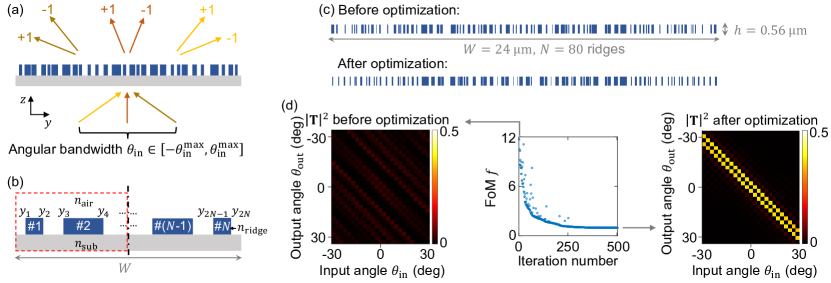
Figure 2: Inverse design of a broad-angle metasurface beam splitter. (a) The desired broad-angle beam-splitting response. (b) Parameter definition and mirror symmetry of the structure. (c) Metasurfaces before and after optimization. (d) Evolution of the FoM of Eq. (5) during optimization and the squared amplitude of the transmission matrices before and after optimization.

As a concrete example, we consider full-wave modeling of the TM fields of a 1200-ridge aperiodic metasurface in 2D with mirror symmetry regarding its central plane ($W=1200\lambda$ wide, $L=0.6\lambda$ thick, discretized with grid size $\Delta x=\lambda/40$ where $\lambda$ is the wavelength), computing its full transmission matrix with $M_{\rm in}=M_{\rm out}=2W/\lambda=2400$ plane-wave channels on each side and the gradient of the transmission matrix with respect to $N_{p}=1200$ parameters being the edge positions of the ridges within half of the metasurface. Here, $\mathrm{nnz}(\mathbf{A})\approx 1.6\times 10^{7}$, and $M_{p}=57600$. Compared to the conventional adjoint method, APF with $N_{\rm sub}=15$ reduces the gradient evaluation time from 1354 minutes to 9.5 minutes and the memory usage from 10 GiB to 7 GiB. Here, the conventional adjoint simulations are also performed with software MESTI [34], which is already optimized by using the efficient MUMPS package [35], utilizing the symmetry of the Maxwell operator matrix ${\bf A}$ and the sparsity of the input profiles. All computations run on a single core on an Intel Xeon 2640v4 node. Details are provided in Sec. 1 of the Supplement 1, Table S1 shows the breakdown of the computing times, and Fig. S1 plots the dependence on $N_{\rm sub}$. We have made our gradient computation code open-source [36], including both the APF version and the conventional adjoint version.

III Inverse design of a broad-angle metasurface beam splitter

As an example, here we inverse design a 2D metasurface beam splitter for TM polarization, composed of ridges with different widths, shown in Fig. 2a. We want the metasurface to split the incident light equally into the $\pm 1$ diffraction orders for any incident angle $\theta_{\rm in}$ within a $2\theta_{\rm in}^{\rm max}$ angular range. Such a broad-angle beam splitter can be used with a vertical-cavity surface-emitting laser (VCSEL) array and a microlens array as a dot projector to generate structured illumination useful for structured illumination microscopy [37, 38], 3D endoscopy [39, 40], and 3D sensing (e.g., facial recognition [41], motion detection [42]). The microlens array collimates the output from the VCSEL array, and the beam splitter increases the number of dots. VCSEL arrays are widely used for dot projectors due to their uniform intensity pattern, high power density, low cost, and simple packaging. However, existing beam splitters based on Dammann gratings [43, 44] or metasurfaces [45, 46, 47] only operate on normal incident light and not the oblique incidence from the off-axis VCSEL units.

We let the metasurface be periodic with the width of one period being $W=24$ µm, which couples transverse angular momenta $k_{y}$ differing by integer multiples of $2\pi/W$. Within the width $W$, we place $N=80$ amorphous-silicon ridges ($n_{\rm ridge}=3.70$) with height $h=0.56$ µm and varying widths and positions, sitting on a silica ($n_{\rm sub}=1.45$) substrate and surrounded by air ($n_{\rm air}=1$), as shown in Fig. 2b,c. The ridge height ensures a sufficient 2$\pi$ range of phase shifts when varying the ridge width (Supplementary Sec. 2 and Fig. S2). Since the desired response is symmetric, we let the structure be mirror symmetric with respect to a central plane at $y=0$ (black dot-dashed line). The operating wavelength is $\lambda=940$ nm, typical for VCSELs. The angular range is $2\theta_{\rm in}^{\rm max}=60^{\circ}$, typical for dot projectors.

To inverse design this broad-angle beam splitter, we minimize the following FoM

$$f[{\bf T}({\bf p}),{\bf p}]=\sum_{n=1}^{M_{\rm out}}\sum_{m=1}^{M_{\rm in}}\left||T_{nm}({\bf p})|^{2}-T_{nm,{\rm target}}^{2}\right|^{2},$$ (5)

where $T_{nm}$ is the transmission coefficient from the $m$-th incident angle to the $n$-th outgoing angle. Here, ${\bf p}=\{p_{k}\}=\{y_{1},\cdots,y_{N}\}$ parameterize the two edge positions of the $N/2$ ridges within half a period of the metasurface [encircled by the red box in Fig. 2b], with $\{y_{N+1},\cdots,y_{2N}\}=-\{y_{N},\cdots,y_{1}\}$ based on symmetry. The target transmission is $T_{nm,{\rm target}}^{2}=0.5$ at the $\pm 1$ diffraction orders and $T_{nm,{\rm target}}^{2}=0$ otherwise. Equation (5) sums over all incident angles within the angular range of interest [i.e., $|k_{y}^{m}|<(2\pi/\lambda)\sin{\theta_{\rm in}^{\rm max}}$ with $2\pi/W$ spacing] and all outgoing angles. With $W=24$ µm, we have $M_{\rm in}=25$ input channels within the $60^{\circ}$ angular range and $M_{\rm out}=51$ output channels. For this specific FoM, $\partial f/\partial p_{k}=0$ and $\partial f/\partial T_{nm}=2(|T_{nm}|^{2}-T_{nm,{\rm target}}^{2})T_{nm}^{*}$ with ^∗ standing for complex conjugation. Here, $\mathrm{nnz}(\mathbf{A})\approx 3.3\times 10^{5}$, and $M_{p}=3840$. Using the APF method above, each objective-plus-gradient evaluation with $N_{\rm sub}=3$ takes 1.6 seconds while using 0.2 GiB of memory when running on one core. To validate that there is no mistake in our derivation and implementation, we show in Fig. S3 that the gradient computed with APF agrees with a brute-force finite-difference evaluation of the FoM in Eq. (5).

To minimize the FoM, we use gradient-based algorithms to update optimization variables $\bf p$ along the opposite direction of the gradient $\bm{\nabla}_{\bf p}f$. The optimizations stop when the change of $f$ is less than $f_{\rm tol}^{\rm abs}=10^{-4}$. After comparing four different algorithms (Supplementary Sec. 4 and Fig. S4), we choose the sequential least-squares quadratic programming (SLSQP) algorithm [48] implemented in the open-source package NLopt [49] since it typically converges the fastest and often to a lower local minimum. During the optimization, the separation between neighboring edges (both the ridge width and the spacing between ridges) is constrained to be at least 40 nm to ensure fabrication feasibility.

We find that randomly sampled configurations of the parameter $\bf p$ have a poor performance with the FoM narrowly distributed between 10 and 20, but SLSQP optimization using those configurations as the initial guess leads to a wide distribution of the optimized FoM (Fig. 3). Since this inverse-design problem is non-convex, there is a sensitive dependence on the initial guess. To find a good final design, we run SLSQP optimizations with 1000 different initial guesses.

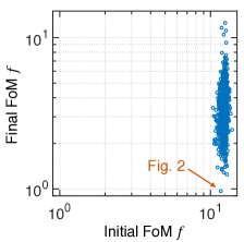
Figure 3: The final FoM and the initial FoM for 1000 randomly generated initial configurations.

Figure 2c,d shows the initial configuration, the final configuration, their corresponding transmission matrices, and the evolution of the FoM for the best case among these optimizations. The optimized metasurface exhibits uniform and near-perfect beam splitting for all incident angles within the $60^{\circ}$ angular range of interest. Here, $|T_{nm}|^{2}$ averages to 0.4 at the $\pm 1$ diffraction orders and to 0.003 away from these angles. Supplementary Video 1 shows how the configuration and the transmission matrix evolve, and Table S2 lists the parameters of the final configuration.

In Sec. 6 and Figs. S6–S7 of the Supplement 1, we consider optimizations where we do not impose a mirror symmetry in the structure. While such a setup is more general, it has a larger-than-necessary design space and yields slightly less optimal results.

IV Outlook

Computer-automated design and discovery unlock numerous possibilities, and the formalism proposed here can be the enabling element for inverse design on a wide range of multi-channel optical systems mentioned in the introduction. Instead of the $N_{\rm sub}$ matrix division employed here, future work may also explore computing the Schur complement of a rectangular augmented matrix to avoid computing the unnecessary matrix $\mathbf{U^{\rm T}A}^{-1}\mathbf{U}$. Advances in the computation method, together with open-source codes, can deliver the next generation of photonic devices.

References

- Jensen and Sigmund [2011] J. S. Jensen and O. Sigmund, Topology optimization for nano-photonics, Laser Photonics Rev. 5, 308 (2011).
- Miller [2012] O. D. Miller, Photonic design: From fundamental solar cell physics to computational inverse design (University of California, Berkeley, 2012).
- Molesky et al. [2018] S. Molesky, Z. Lin, A. Y. Piggott, W. Jin, J. Vucković, and A. W. Rodriguez, Inverse design in nanophotonics, Nat. Photonics 12, 659 (2018).
- Elsawy et al. [2020] M. M. Elsawy, S. Lanteri, R. Duvigneau, J. A. Fan, and P. Genevet, Numerical optimization methods for metasurfaces, Laser Photonics Rev. 14, 1900445 (2020).
- Fan [2020] J. A. Fan, Freeform metasurface design based on topology optimization, MRS Bull. 45, 196 (2020).
- Li et al. [2022] Z. Li, R. Pestourie, Z. Lin, S. G. Johnson, and F. Capasso, Empowering metasurfaces with inverse design: Principles and applications, ACS Photonics 9, 2178 (2022).
- Yang and Vuckovic [2023] K. Yang and J. Vuckovic, Special issue on “Optimized photonics and inverse design”, ACS Photonics 10, 801 (2023).
- Lin et al. [2021] Z. Lin, C. Roques-Carmes, R. E. Christiansen, M. Soljačić, and S. G. Johnson, Computational inverse design for ultra-compact single-piece metalenses free of chromatic and angular aberration, Appl. Phys. Lett. 118, 041104 (2021).
- Bogaerts et al. [2020] W. Bogaerts, D. Pérez, J. Capmany, D. A. Miller, J. Poon, D. Englund, F. Morichetti, and A. Melloni, Programmable photonic circuits, Nature 586, 207 (2020).
- Lin et al. [2018] Z. Lin, B. Groever, F. Capasso, A. W. Rodriguez, and M. Lončar, Topology-optimized multilayered metaoptics, Phys. Rev. Appl. 9, 044030 (2018).
- Li and Hsu [2022] S. Li and C. W. Hsu, Thickness bound for nonlocal wide-field-of-view metalenses, Light Sci. Appl. 11, 338 (2022).
- Li and Hsu [2023] S. Li and C. W. Hsu, Transmission efficiency limit for nonlocal metalenses, arXiv:2303.00726 (2023).
- Cheng et al. [2017] J. Cheng, S. Inampudi, and H. Mosallaei, Optimization-based dielectric metasurfaces for angle-selective multifunctional beam deflection, Sci. Rep. 7, 12228 (2017).
- Liu et al. [2021] Z. Liu, W. Feng, Y. Long, S. Guo, H. Liang, Z. Qiu, X. Fu, and J. Li, A metasurface beam combiner based on the control of angular response, Photonics 8, 489 (2021).
- Kamali et al. [2017] S. M. Kamali, E. Arbabi, A. Arbabi, Y. Horie, M. Faraji-Dana, and A. Faraon, Angle-multiplexed metasurfaces: Encoding independent wavefronts in a single metasurface under different illumination angles, Phys. Rev. X 7, 041056 (2017).
- Jang et al. [2021] J. Jang, G.-Y. Lee, J. Sung, and B. Lee, Independent multichannel wavefront modulation for angle multiplexed meta-holograms, Adv. Opt. Mater. 9, 2100678 (2021).
- Roques-Carmes et al. [2022] C. Roques-Carmes, Z. Lin, R. E. Christiansen, Y. Salamin, S. E. Kooi, J. D. Joannopoulos, S. G. Johnson, and M. Soljacic, Toward 3D-printed inverse-designed metaoptics, ACS Photonics 9, 43 (2022).
- Rodriguez et al. [2011] A. W. Rodriguez, O. Ilic, P. Bermel, I. Celanovic, J. D. Joannopoulos, M. Soljačić, and S. G. Johnson, Frequency-selective near-field radiative heat transfer between photonic crystal slabs: a computational approach for arbitrary geometries and materials, Phys. Rev. Lett. 107, 114302 (2011).
- Rodriguez et al. [2013] A. W. Rodriguez, M. H. Reid, and S. G. Johnson, Fluctuating-surface-current formulation of radiative heat transfer: theory and applications, Phys. Rev. B 88, 054305 (2013).
- Yao et al. [2022] W. Yao, F. Verdugo, R. E. Christiansen, and S. G. Johnson, Trace formulation for photonic inverse design with incoherent sources, Struct. Multidiscip. Optim. 65, 336 (2022).
- Zhu et al. [2017] T. Zhu, Y. Zhou, Y. Lou, H. Ye, M. Qiu, Z. Ruan, and S. Fan, Plasmonic computing of spatial differentiation, Nat. Commun. 8, 15391 (2017).
- Kwon et al. [2018] H. Kwon, D. Sounas, A. Cordaro, A. Polman, and A. Alù, Nonlocal metasurfaces for optical signal processing, Phys. Rev. Lett. 121, 173004 (2018).
- Guo et al. [2018] C. Guo, M. Xiao, M. Minkov, Y. Shi, and S. Fan, Photonic crystal slab Laplace operator for image differentiation, Optica 5, 251 (2018).
- Cordaro et al. [2019] A. Cordaro, H. Kwon, D. Sounas, A. F. Koenderink, A. Alù, and A. Polman, High-index dielectric metasurfaces performing mathematical operations, Nano Lett. 19, 8418 (2019).
- Zhou et al. [2020a] Y. Zhou, H. Zheng, I. I. Kravchenko, and J. Valentine, Flat optics for image differentiation, Nat. Photonics 14, 316 (2020a).
- Zhou et al. [2020b] J. Zhou, S. Liu, H. Qian, Y. Li, H. Luo, S. Wen, Z. Zhou, G. Guo, B. Shi, and Z. Liu, Metasurface enabled quantum edge detection, Sci. Adv. 6, eabc4385 (2020b).
- Xue and Miller [2021] W. Xue and O. D. Miller, High-NA optical edge detection via optimized multilayer films, J. Opt. 23, 125004 (2021).
- Silva et al. [2014] A. Silva, F. Monticone, G. Castaldi, V. Galdi, A. Alù, and N. Engheta, Performing mathematical operations with metamaterials, Science 343, 160 (2014).
- Zangeneh-Nejad et al. [2021] F. Zangeneh-Nejad, D. L. Sounas, A. Alù, and R. Fleury, Analogue computing with metamaterials, Nat. Rev. Mater. 6, 207 (2021).
- Guo et al. [2020] C. Guo, H. Wang, and S. Fan, Squeeze free space with nonlocal flat optics, Optica 7, 1133 (2020).
- Reshef et al. [2021] O. Reshef, M. P. DelMastro, K. K. Bearne, A. H. Alhulaymi, L. Giner, R. W. Boyd, and J. S. Lundeen, An optic to replace space and its application towards ultra-thin imaging systems, Nat. Commun. 12, 3512 (2021).
- Chen and Monticone [2021] A. Chen and F. Monticone, Dielectric nonlocal metasurfaces for fully solid-state ultrathin optical systems, ACS Photonics 8, 1439 (2021).
- Lin et al. [2022] H.-C. Lin, Z. Wang, and C. W. Hsu, Fast multi-source nanophotonic simulations using augmented partial factorization, Nat. Comput. Sci. 2, 815 (2022).
- [34] H.-C. Lin, Z. Wang, and C. W. Hsu, MESTI, https://github.com/complexphoton/MESTI.m.
- Amestoy et al. [2001] P. R. Amestoy, I. S. Duff, J. S. Koster, and J.-Y. L’Excellent, A fully asynchronous multifrontal solver using distributed dynamic scheduling, SIAM J. Matrix Anal. Appl. 23, 15–41 (2001).
- [36] S. Li and C. W. Hsu, APF Inverse Design, https://github.com/complexphoton/APF_inverse_design.
- Gustafsson [2000] M. G. Gustafsson, Surpassing the lateral resolution limit by a factor of two using structured illumination microscopy, J. Microsc. 198, 82 (2000).
- Gustafsson [2005] M. G. Gustafsson, Nonlinear structured-illumination microscopy: wide-field fluorescence imaging with theoretically unlimited resolution, Proc. Natl. Acad. Sci. U.S.A. 102, 13081 (2005).
- Furukawa et al. [2016a] R. Furukawa, Y. Sanomura, S. Tanaka, S. Yoshida, R. Sagawa, M. Visentini-Scarzanella, and H. Kawasaki, 3D endoscope system using DOE projector, in 2016 38th Annual International Conference of the IEEE Engineering in Medicine and Biology Society (EMBC) (IEEE, 2016) pp. 2091–2094.
- Furukawa et al. [2016b] R. Furukawa, H. Morinaga, Y. Sanomura, S. Tanaka, S. Yoshida, and H. Kawasaki, Shape acquisition and registration for 3D endoscope based on grid pattern projection, in Computer Vision–ECCV 2016: 14th European Conference, Amsterdam, The Netherlands, October 11-14, 2016, Proceedings, Part VI 14 (Springer, 2016) pp. 399–415.
- Kwon et al. [2021] J.-M. Kwon, S.-P. Yang, and K.-H. Jeong, Stereoscopic facial imaging for pain assessment using rotational offset microlens arrays based structured illumination, Micro Nano Syst. Lett. 9, 11 (2021).
- Dutta [2012] T. Dutta, Evaluation of the Kinect™ sensor for 3-D kinematic measurement in the workplace, Appl. Ergon. 43, 645 (2012).
- Li et al. [2015] Z. Li, G. Zheng, S. Li, Q. Deng, J. Zhao, Y. Ai, et al., All-silicon nanorod-based Dammann gratings, Opt. Lett. 40, 4285 (2015).
- Yang et al. [2017] S. Yang, C. Li, T. Liu, H. Da, R. Feng, D. Tang, F. Sun, and W. Ding, Simple and polarization-independent Dammann grating based on all-dielectric nanorod array, J. of Opt. 19, 095103 (2017).
- Li et al. [2018] Z. Li, Q. Dai, M. Q. Mehmood, G. Hu, B. L. yanchuk, J. Tao, C. Hao, I. Kim, H. Jeong, G. Zheng, et al., Full-space cloud of random points with a scrambling metasurface, Light Sci. Appl. 7, 63 (2018).
- Song et al. [2018] X. Song, L. Huang, C. Tang, J. Li, X. Li, J. Liu, Y. Wang, and T. Zentgraf, Selective diffraction with complex amplitude modulation by dielectric metasurfaces, Adv. Opt. Mater. 6, 1701181 (2018).
- Ni et al. [2020] Y. Ni, S. Chen, Y. Wang, Q. Tan, S. Xiao, and Y. Yang, Metasurface for structured light projection over 120 field of view, Nano Lett. 20, 6719 (2020).
- Kraft [1994] D. Kraft, Algorithm 733: TOMP–Fortran modules for optimal control calculations, ACM Trans. Math. Softw. 20, 262 (1994).
- [49] S. G. Johnson, The NLopt Nonlinear-Optimization Package, https://github.com/stevengj/nlopt.