On Selecting Distance Metrics in $n$-Dimensional Normed Vector Spaces of Cells: A Novel Criterion and Similarity Measure Towards Efficient and Accurate Omics Analysis

Abstract

Single-cell omics enable the profiles of cells, which contain large numbers of biological features, to be quantified. Cluster analysis, a dimensionality reduction process, is used to reduce the dimensions of the data to make it computationally tractable. In these analyses, cells are represented as vectors in $n$-Dimensional space, where each dimension corresponds to a certain cell feature. The distance between cells is used as a surrogate measure of similarity, providing insight into the cell’s state, function, and genetic mechanisms. However, as cell profiles are clustered in 3D or higher-dimensional space, it remains unknown which distance metric provides the most accurate spatiotemporal representation of similarity, limiting the interpretability of the data. I propose and prove a generalized proposition and set of corollaries that serve as a criterion to determine which of the standard distance measures is most accurate for conveying cell profile heterogeneity. Each distance method is evaluated via statistical, geometric, and topological proofs, which are formalized into a set of criteria. In this paper, I present the putative, first-ever method to elect the most accurate and precise distance metrics with any profiling modality, which are determined to be the Wasserstein distance and cosine similarity metrics, respectively, in general cases. I also identify special cases in which the criterion may select non-standard metrics. Combining the metric properties selected by the criterion, I develop a novel, custom, optimal distance metric that demonstrates superior computational efficiency, peak annotation, motif identification, and footprinting for transcription factor binding sites when compared with leading methods.

1 Introduction

The DNA in mammalian cells is highly condensed through three major hierarchical classifications: a basic, repeating nucleosome subunit that coils into the chromatin complexes, which comprise the chromosome. Chromatin exists in a euchromatin form, which is transcriptionally active, and a heterochromatin form, which cannot be transcribed [1, 2]. Together, these DNA condensation hierarchies are the major determinants of gene regulation [3, 4, 5, 6, 7]. Single-cell analysis technologies are therefore used to study the biological features of individual cells to provide insight into their genetic regulatory activity; they are key to assessing the genome-wide characteristics of these cells for biochemical and epidemiological applications, such as disease state modeling and prediction, therapeutics, and genetic profiling [8, 9, 10, 11, 12]. High-throughput single-cell omics data is often highly heterogeneous, noisy, and sparse, containing multiple features, making dimensionality reduction techniques necessary for visualizing results [13, 14, 15, 16]. Single-cell sequencing methods aim to highlight cellular heterogeneity at large, as observing such differences on a cell-to-cell scale allows for the identification of new and more precise cell subpopulations for the high-fidelity characterization of dense biological data.

Identification of the optimal distance metric allows for several downstream analysis methods, such as identifying global structure and sub-structure from the sequencing, determining biological patterns, and assessing whole-genome etiologies of cellular disease states [17]. The dynamic field of omics technology has continued to streamline the development of techniques to interrogate DNA, chromatin, mRNA, and protein modalities, such as ATAC-Seq and PIP-seq, which rely on quality single-cell clustering to produce accurate cell-cell distances. However, current computational pipelines for calculating intercluster distances do not account for dropout events, sparsity, or obscured dissimilarity, which results in several missing data. Distance metrics, or methods of calculating distance, inform the reliability of biological and epigenetic findings yielded from the recorded cell profiles. Thus, distance effectively serves as a measure of similarity between cells, in which smaller distances indicate higher levels of similarity and vice versa. However, it is currently unknown which metric is best suited to represent the distance between cells within a high-dimensional cluster.

Prior literature has explored the selection of appropriate distances in clustering, but these studies do not offer generalizable conclusions, instead providing selection criteria of a certain distance metric in an isolated context such as gene expression divergence [18, 19] or provide recommendations for a certain class of calculations, such as proportionality-based metrics [20, 21, 22]. There appears to be no consensus within existing literature of the same flavor, however, with each study concluding different types of distance metrics as being the most effective. It has been determined that the structural properties of omics data have an influence on the performance of dimensionality reduction and distance metrics, so it is reasonably inferred that results from previous work do not generalize, which may explain the discrepancy in results [23, 24, 25]. For example, rare cell populations only have minute genetic differences from their abundant, stable counterparts and are therefore often undetected by traditional metrics. A leading solution to these caveats is Optimal Transport (OT), the noncanonical version of the Wasserstein distance, in which distances in high dimensional data are represented as probability distributions, and the OT finds a coupling between them that minimizes transportation cost [26, 27, 28, 29]. However, OT exhibits low-resolution conservation of global structure and cellular features, indicating that while it may be effective in identifying cell-cell similarity, the quality of the molecular profiles of each cell significantly reduces [30, 31, 32, 33, 34]. The lack of an effective selection criterion in single-cell omics workflows has limited the specificity and utility of the findings yielded from cell profiling.

I present a novel distance selection criterion that is able to accurately determine the best distance metric to convey cell-cell similarity while maintaining the maximum amount of feature specificity within the data so as to identify heterogeneity in cell subpopulations, mutation loci in non-coding regions, and functional differences in cells, i.e. the presence of open chromatin. This method uniquely elects distance metrics by considering the structure of the data, applied feature extraction techniques, and the biological modalities being measured. Such a holistic approach results in superior sensitivity, specificity, and accuracy in single-cell omics, enabling a high-resolution view and identification of functional changes at the cellular level across cell types and conditions such as disease states or gene knockout.

In this study, I rigorously prove the mathematical ground truth of this method, then assess the efficiency of my method in comparison with OT. The criterion is applied to data from whole-genome sequenced spinal and cranial motor neurons using the single-cell Assay for Transposase-Accessible Chromatin (scATAC-Seq), which determines cellular chromatin state, a hallmark of cis-regulatory activity [35]. I extrapolate from the chromatin accessibility landscape of each cell to identify subclusters of new cell types and the loci of non-coding mutations in KIF21A (kinesin family member 21A), TUBB3 (tubulin beta 3 class III), MAFB (MAF BZIP Transcription Factor B), and CHN1 (Hchimerin 1) genes, which have been implicated in congenital cranial dysinnervation disorders (CCDDs), a class of neurogenic conditions. These findings provide insights into the genetic causes of CCDDs and their effects on varying neuron types and demonstrate the robustness of the distance selection criterion.

2 Materials and Methods

2.1 Cell Profiling Data

Single-cell ATAC-Seq was performed on a set of 85,089 purified spinal and cranial motor neurons in varying levels of embryonic development, which served as a ground truth for this study. The neurons were sourced from mouse models with two KIF21A, two TUBB3, CHN1, MAFB, and TWIST1 human missense mutations, each corresponding to four CCDD phenotypes: ptosis, Duane Syndrome, congenital fibrosis of the extraocular muscles (CFEOM), and craniocytosis. The dataset also included wild-type lab mice. ATAC-Seq generated 255,804 chromatin-accessible peaks, with high sample-level concordance across biological and technical replicates as well as ground truth data generated from gold standard fluorescence-activated cell sorting (FACS) labels and bulk experiments. I organized the data sequentially by embryonic age.

2.2 Distance Selection Criteria

We annotate the sequenced cells with a unique barcode, tissue type, replicate type, and embryonic age (denoted as time $e$). These data comprise a ‘prefix’ that describes the cell’s identity. For example, a cranial motor neuron 7 with an embryonic age of 11.5 in the third batch of profiling would be denoted CN7-R3-$e$11-5, while its biological and technical replicates would be notated as CN7-R2-$e$11-5 and CN7-R3T-$e$10-5, respectively, where biological replicates represent parallel measurements of biologically distinct samples that capture random biological variation or noise, while technical replicates represent repeated measurements of the same sample, capturing random noise associated with the experiment.

The ground-truth labels within the data demonstrate a high correlation between the biological profiles of replicates—technical replicates and biological replicates are more similar than non-replicates and therefore have closer proximity in clustering—that holds in a generalized context. Thus, I conclude Proposition 2.1:

Proposition 2.1.

Given a cell pair, $\oplus^{\prime}$, of an original cell and its technical replicate, a second cell pair, $\oplus$, of the same original cell and its biological replicate, and a final cell pair, $\succ$, of the same original cell and a non-replicate, $d\left(\oplus^{\prime}\right)<d\left(\oplus\right)<d\left(\succ\right)$.

Proof.

Assume a set $C_{\tau}$ containing all technical replicate pairs, another set $C_{\beta}$ containing all $\oplus$, and a final set $C_{1}$ containing all $\succ$. Assume that $C_{\tau}$, $C_{\beta}$, and $C_{1}$ overlap in all clusters, but are "hard", such that they exhibit distinct pairwise distance patterns that can be related to one another. Therefore, the $m\times n$ similarity matrices of each of the cells in the sets are defined as:

$$S_{{\tau}_{C_{\tau}}}=\begin{bmatrix}S_{{\tau}_{11}}&S_{{\tau}_{12}}&\cdots&S_{{\tau}_{1j}}&\cdots&S_{{\tau}_{1n}}\\ S_{{\tau}_{i1}}&S_{{\tau}_{i2}}&\cdots&S_{{\tau}_{ij}}&\cdots&S_{{\tau}_{in}}\\ S_{{\tau}_{m1}}&S_{{\tau}_{m2}}&\cdots&S_{{\tau}_{mj}}&\cdots&S_{{\tau}_{mn}}\end{bmatrix}\textnormal{, }S_{{\beta}_{C_{\beta}}}=\begin{bmatrix}S_{{\beta}_{11}}&S_{{\beta}_{12}}&\cdots&S_{{\beta}_{1j}}&\cdots&S_{{\beta}_{1n}}\\ S_{{\beta}_{i1}}&S_{{\beta}_{i2}}&\cdots&S_{{\beta}_{ij}}&\cdots&S_{{\beta}_{in}}\\ S_{{\beta}_{m1}}&S_{{\beta}_{m2}}&\cdots&S_{{\beta}_{mj}}&\cdots&S_{{\beta}_{mn}}\end{bmatrix}\textnormal{, }$$

and $S_{{\succ}_{C_{1}}}=\begin{bmatrix}S_{{\succ}_{11}}&S_{{\succ}_{12}}&\cdots&S_{{\succ}_{1j}}&\cdots&S_{{\succ}_{1n}}\\ S_{{\succ}_{i1}}&S_{{\succ}_{i2}}&\cdots&S_{{\succ}_{ij}}&\cdots&S_{{\succ}_{in}}\\ S_{{\succ}_{m1}}&S_{{\succ}_{m2}}&\cdots&S_{{\succ}_{mj}}&\cdots&S_{{\succ}_{mn}}\end{bmatrix}$.

where $S$ is a similarity coefficient, and $i$ and $j$ are features in which $S$ determines similarity. Given that an ordered pair of cells in $\oplus^{\prime}$, $(c_{0},c_{\tau})$, must contain features $i\approxeq j$ more than in $(c_{0},c_{\beta})$, and cells in pair $\oplus$ must contain features $i\approx j$ significantly more than in $\succ$, given their biological properties, we can use the similarity matrices to compare the pairwise distances between the cell pairs. First, we note that the matrix $S_{{\tau}{C{\tau}}}$ contains similarity coefficients between technical replicates, and we assume that each of these coefficients is small. Similarly, we assume that the similarity coefficients between biological replicates in the matrix $S_{{\beta}{C{\beta}}}$ are relatively large.

Next, we note that the matrix $S_{{\succ}{C{1}}}$ contains similarity coefficients between the non-replicate cell and the original cell. We assume that these coefficients are larger than those in $S_{{\tau}{C{\tau}}}$, but smaller than those in $S_{{\beta}{C{\beta}}}$. Using the identity of indiscernibles in a normed vector space, we can show that $d\left(\oplus^{\prime}\right)<d\left(\oplus\right)<d\left(\succ\right)$. This is because the features that are more similar in the technical replicates and biological replicates are smaller in magnitude than those that are more similar in the non-replicate cell and the original cell. Therefore, the distance between the technical replicates is smaller than the distance between the biological replicates, which is in turn smaller than the distance between the non-replicate cell and the original cell. So, $d\left(\oplus^{\prime}\right)<d\left(\oplus\right)<d\left(\succ\right)$ in all general cases. ∎

In any given area within the metric space, $X_{\textnormal{cells}}$, formed by the clustering of sequenced cells, there are $\oplus^{\prime},\oplus,\textnormal{and}\succ$ pairs. Given that generally, the distances between these pairs adhere to a hierarchy of length, several properties describing the clusters in $X_{\textnormal{cells}}$ arise out of Proposition 2.1, which account for global data structure and biological features.

Corollary 1.

In any area of $X_{\textnormal{cells}}$, there are points $c_{0},c_{\tau}$ in the pair $\oplus^{\prime}$, $c_{0},c_{\beta}$ in the pair $\oplus$, and $c_{0},c_{1}$ in the pair $\succ$, where $c_{0}$ and $c_{1}$ are distinct cell types and $c_{\tau},c_{\beta}$ are technical and biological replicates of $c_{0}$. Therefore, $X_{\textnormal{cells}}$ always defines a “weak” complete metric space of points in $\mathbb{R}^{n}$:

$$\begin{split}\forall c_{0}\neq c_{\beta}\neq c_{\tau}\in X_{\textnormal{cells}}.\,\,\exists\,\,c_{1}\in X_{\textnormal{cells}}.\,\,d(c_{0},c_{\tau})<d(c_{0},c_{1})&\wedge d(c_{\tau},c_{\beta})<d(c_{0},c_{\beta})\\ &\wedge d(c_{\beta},c_{1})<d(c_{\tau},c_{1}),\end{split}$$

which forms a topological manifold $M_{\textnormal{cells}}$.

On the manifold $M_{\textnormal{cells}}$, each point is a 0-D manifold. Therefore, at any given point, the geometry in its local neighborhood appears Euclidean [36]. However, other distance metrics can be used to calculate the distance between points on the manifold. Corollary 1 describes the topology of the metric space $X_{\textnormal{cells}}$, from which I obtain a new corollary that describes the extrema of pairwise distances of the manifold.

Corollary 2.

The most precise distance metric, $d_{\textnormal{p}}$ optimizes for the hierarchical ordering of lengths between pairs on $M_{\textnormal{cells}}$, $d\left(\oplus^{\prime}\right)<d\left(\oplus\right)<d\left(\succ\right)$, such that $d_{\textnormal{p}}(\oplus^{\prime})=\textnormal{min}(c_{0},c_{\tau})$ and $d_{\textnormal{p}}(\succ)=\textnormal{max}(c_{0},c_{1}).$

In Corollary 2, the best metric $d$ is said to optimize for the maximum distance between unrelated cells, and the minimum distance between highly related cells. Replicates must also follow some consistent correlation, and an optimal metric can identify such minute differences. I obtain an average function transformation value between biological and technical replicates when converting the distributions of their calculated distances with any modality or distance metric to a Gaussian function, given the dataset follows Proposition 2.1:

Corollary 3.

Comparing coordinates from distance metrics normalized within the bounds [0,1], with a mean value $\mu=0$ and standard deviation $\sigma=0$, a distance $d$ is accurate in relative space
if $d(c_{0},c_{\beta})\approx 1.02d(c_{0},c_{\tau})$. The metric that approaches a function transformation of 0.02 between $\oplus^{\prime}$ and $\oplus$ pairwise distances most closely is called $d_{\textnormal{a}}$.

Remark.

It is possible that $d_{\textnormal{a}}\neq d_{\textnormal{p}}$, however, it is likely that the Pearson correlation $r<0.05$ (positive correlation) between the two distances. Given the high probability of statistically significant correlation between the two distances, it is also likely that $d_{\textnormal{a}}\approx d_{\textnormal{p}}$ or $d_{\textnormal{a}}=d_{\textnormal{p}}$, but there are no cases in which $d_{\textnormal{a}}$ must equal $d_{\textnormal{p}}$.

Finally, I observe the features and dimensions of the selected metrics to ensure the criterion’s robustness to increased resolution and a method of calculating statistical significance that follows the ground truth. Given the relationship between distance and replicate similarity, I confirm the statistical similarity between biological and technical replicates. I then assume that as more features (entries within the probability distribution of distances) are added to the Gaussian functions of $d_{\textnormal{a}}$ and $d_{\textnormal{p}}$, they approach a transformation value of 0.02 across all dimensions more closely:

Corollary 4.

In any n-Dimensional norm-induced metric space, $d_{\textnormal{a}}$ and $d_{\textnormal{p}}$ will have a strong, linear statistical correlation $r\gtrapprox 0.90$. In cases where $d_{\textnormal{a}}\veebar d_{\textnormal{b}}$ is a similarity measure, $d_{\textnormal{a}}$ and $d_{\textnormal{p}}$ will have a Pearson correlation , and therefore highly similar geometries.

Corollary 5.

Given any $n$-Dimensional real-valued vector space inducing a metric space, the $\lim_{n\to\infty}$ $d_{\textnormal{b}}=d_{\textnormal{a}}$ and $\lim_{n\to\infty}d_{\textnormal{a}}=d_{\textnormal{b}}$, where $d_{\textnormal{b}}(\oplus-\oplus^{\prime})\rightarrow 0.02$ and $d_{\textnormal{a}}(\oplus,\oplus^{\prime})\rightarrow(\textnormal{min},\textnormal{max})$, respectively.

2.3 Criteria-Informed Metrics

2.3.1 Pairwise Similarity Tests Establish the Wasserstein Distance and Cosine Similarity as $d_{\textnormal{b}}$ and $d_{\textnormal{a}}$

Here, I utilize the developed criteria to determine which out of 9 standard baseline metrics—cosine similarity [37], the Wasserstein [38], Optimal Transport, and Hamming [39] distances, the Pearson and Spearman correlations, as well as the Minkowski distance’s three emergent cases: the Manhattan [40], Euclidean [41], and Chebyshev [42] distances—behave most closely to $d_{\textnormal{b}}$ and $d_{\textnormal{a}}$ in general cases.

I begin by obtaining new peaks from the ground truth peaks generated in the data set from each standard metric, then constructing a count matrix from the peaks scores to create cluster matrices and their corresponding visualizations, and then performing downstream analysis to characterize TF motifs and open chromatin scores across cells (Figure 1A). From these data, I then compare a subset of all pairwise distances of the sequenced cells from each metric, then iterate through the rows of the scATAC-Seq data directly, calculating the distances of each adjacent cell using each of the spatial coordinates from each standard distance metric. These spatial coordinates represent the clustering of the cells based on their chromatin accessibility, as defined by the sequencing. The clustering coordinates are obtained via Uniform Manifold Approximation and Projection (UMAP) [43]. The UMAP algorithm takes an input of an ATAC-Seq dataset $D$ in a high dimensional space $\mathbb{R}^{n}$ and converts it to its low-dimensional analog $\mathbb{R}^{m}$ via an embedding $\phi$ [44, 45, 46, 47, 48]. Each of these data points is drawn from $M_{\textnormal{cells}}$, such that every point in $D$ is connected to $M_{\textnormal{cells}}$. I then remove the manifold trace and leave only clusters of points from $D$, grouped based on different measures of biological similarity. From these data, I find and plot the differences between coordinate values to further analyze the deviations observed in UMAP. I segment by $\oplus^{\prime},\oplus,\textnormal{and}\succ$, finding the distances between the pairs with each metric and plotting their distributions. Normalization of all distances to the range $[0,1]$ is achieved by min-max feature scaling.

The data confirms Corollary 3, as there are minimal differences in the distributions of distances in biological and technical replicates, independent of the metric being used. Converting the distributions of ${d(\oplus^{\prime})}_{m}$ and ${d(\oplus)}_{m}$ to the functions $f_{\tau}$ and $f_{\beta}$, respectively, I find that in all Wasserstein distances $f_{\tau}=0.0443f_{\beta}$ and in all cosine similarity $f_{\tau}=0.0421f_{\beta}$, following that the average difference in distance between points within all metrics will $\approx 0.04$ (Figure 1B, 1C). Due to 0.04 being within statistically significant proximity to 0.02, I use this data to accurately identify $d_{\textnormal{a}}$. Furthermore, as I decrease feature extraction to include more dimensions, I find that the overall distribution of distances decreases to an average function transformation value $f_{\tau}=0.0279f_{\beta}$, per Corollary 4.

From the normalized distance values in $D$, I create and visualize a new dataset $D_{\textnormal{s}}$, which contains the arithmetic difference of all the values to capture disparities in their calculations. $D_{\textnormal{s}}$ contains all the remainders when each distance value of a certain metric is subtracted from the corresponding distances of all other metrics. Within the difference distributions, I uncover high variation between cosine similarity and the Wasserstein distance from all other distance metrics, whereas the Hamming, Euclidean, Minkowski, and Chebyshev distances in particular adhere to less accurate plot patterns. In the difference graphs, the subtracted distances between the four distance measures are also minimized in the graphs of the Wasserstein distance and cosine similarity (Figure 1D, 1E, 1F), which indicates that they are more closely maintaining the distance hierarchy principle of Proposition 2.1 than all other standard metrics.

I record the mean data by a statistic $\bar{\textbf{x}}$, which represents the average of a set of distance values. I find that on average, the cosine similarity values between technical and biological replicates vary by 0.02216, suggesting that it is $d_{\textnormal{a}}$, and the Wasserstein maximizes the distance between $\oplus^{\prime}$ and $\oplus$ pairs, indicating that it is $d_{\textnormal{p}}$. Performing a two-sided chi-square test at an alpha level $\alpha=0.01$, I obtain a chi-square value $\chi^{2}=0.009752$. Since $\chi^{2}<0.01$, it follows that I am 99% confident that the true relatively accurate distance metric $d_{\textnormal{a}}$ is cosine similarity. Performing another two-sided chi-square test, again at $\alpha=0.05$ for Wasserstein, I find that $\chi^{2}$ is again a statistically significant value of 0.029417. Therefore, I am 95% confident that the true most “correct” distance metric, $d_{\textnormal{b}}$, is the Wasserstein distance. Furthermore, I determine that the cosine similarity and Wasserstein distance have a strong, inversely proportional correlation $r=-0.993\pm 0.0492$ .

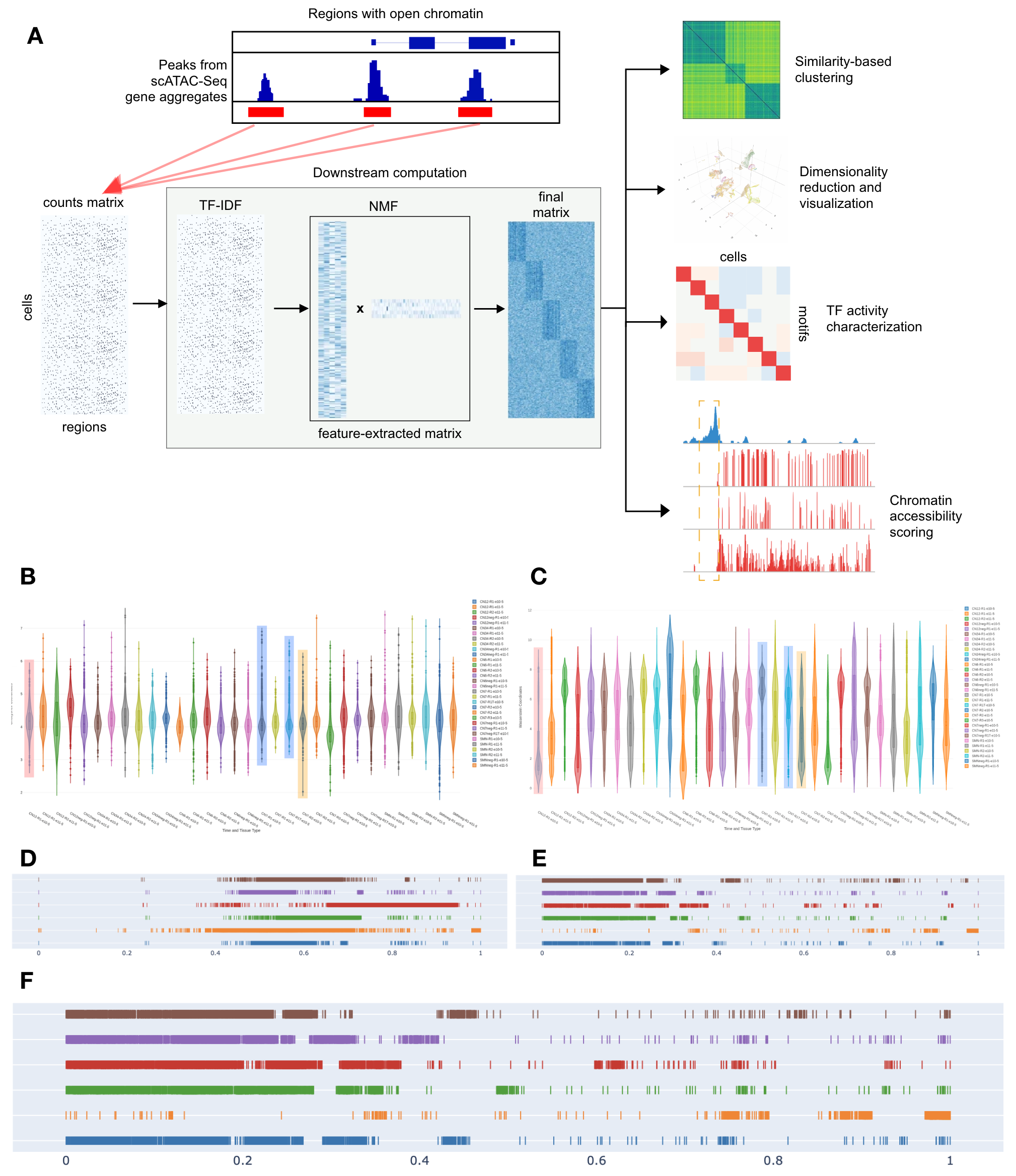
Figure 1: (A) The general ATAC-Seq procedure, where term frequency-inverse document frequency (TF-IDF) and non-negative matrix factorization (NMF) yield a final matrix. (B, C) Violin plots illustrate the distribution of distances in the cosine similarity and Wasserstein distance, respectively. The blue highlight indicates $\oplus^{\prime}$ pairs, the orange represents cells in an $\oplus$ pair, and the red represents cells in a $\succ$ pair. ($\textbf{D},\textbf{E},\textbf{F}$) Arithmetic difference plots of each metric for $d({c_{0},c_{\tau}})$ in $\oplus^{\prime}$, $d({c_{0},c_{\beta}})$ in $\oplus$, and $d({c_{\textnormal{orig}},c_{1}})$ in $\succ$, where the brown is Wasserstein, purple is Hamming, red is Manhattan, green is Euclidean, orange is cosine similarity, and blue is Chebyshev.

I analyze pairwise cell heterogeneity using a variety of data organizations to determine the accuracy of the $d_{\textnormal{a}}$ and $d_{\textnormal{b}}$ metric suspects by parsing the data by the metric-yielded cluster annotation, time, and tissue type. When testing UMAPs ordered by time, cluster, and tissue, the Wasserstein and cosine similarity metrics still yielded the best results, with the Wasserstein having the highest deviation between technical and non-replicates at a normalized $\bar{\textbf{x}}$ value of $\sim 0.7782$, and the cosine similarity metric yielding an average technical and non-replicate distance difference of $\sim 0.6548$ and a function transformation between $d(\oplus^{\prime})$ and $d(\oplus)$ of $\sim$0.0225, whereas the Wasserstein had a shift of $\sim$0.0341, consistent with the aforementioned conclusions on the identity of the $d_{\textnormal{a}}$ and $d_{\textnormal{p}}$ metrics. Furthermore, when the 3-D Wasserstein and cosine similarity normalized UMAPs were placed on top of one another, there were few differences observed in their inverse visual geometries, confirming their high correlation and adherence to Corollary 5.

2.3.2 Unique Geometric and Topological Properties of $d_{\textnormal{b}}$ and $d_{\textnormal{a}}$ UMAPs Confirm Correlation

Current methods to calculate distance within single-cell omics maps do not evaluate the geometric or topological properties of the objects produced by the clustering of cells within a given metric space, and how closely they align with the $n$-Dimensional vector space of the feature extraction itself [49, 50, 51, 52]. As such, methods such as Optimal Transport are not as reliable in general biological settings, as the structure of the embeddings, particularly UMAP, are not considered.

I adopt a novel approach to observe the properties of $d_{\textnormal{a}}$ and $d_{\textnormal{b}}$ concerning their shared geometry. To determine if the cluster maps produced by the Wasserstein distance and cosine similarity fit to $M_{\textnormal{cells}}$, I extract 2-D cross-sections from the images of the UMAP embeddings of single-cell chromatin accessibility profiles produced by each metric, which reflect a similar, inverse geometrical structure (Figure 2D, 2E) when compared to other standard metrics (Figure 2F). Before identifying shared features within the cross-sectional images, I compute the signal-to-noise ratio (SNR) between the pixels of the produced embedding and any ‘background’ pixels in $\widehat{f}$, defined as portions of the original geometry $f$ that do not fit $M_{\textnormal{cells}}$. The larger the proportion of the image that these portions comprise, the lower the SNR value of the distance metric. Therefore, I compute the SNR as an image as in Gonzalez et al.’s root-mean-squared-signal-to-noise ratio [53]:

$$\textnormal{SNR}=\frac{\sum\limits_{x=0}^{M-1}\sum\limits_{y=0}^{N-1}\widehat{f}(x,y)^{2}}{\sum\limits_{x=0}^{M-0}\sum\limits_{y=0}^{N-1}\left[f(x,y)-\widehat{f}(x,y)\right]^{2}}\hskip 14.45377pt$$

This can further be described as the image signal mean $\bar{S}$ subtracted as the image background mean $\bar{B}$ of pixel intensities divided by the standard deviation of the image background $\sigma_{\textnormal{b}}$. From this derivation, I find that in all test cases and across all cell groupings, the SNR is maximized in the Wasserstein distance and cosine similarity. Consequently, less noise (in this case, incorrect geometry) is present when producing clustering images in the metric space (Figure 2A).

Next, using the SNR value as a corrective measure, I truncate the data by cell line and annotation to observe the computed scaled distance values by each metric. Consistent with the aforementioned pairwise similarity tests, I find that the Wasserstein distance one again minimizes the distance between $\oplus^{\prime}$ pairs and maximizes the distance between $\succ$ pairs, while the cosine similarity optimizes for a function transformation of 0.02 between $\oplus^{\prime}$ and $\oplus$ average distance values (Figure 2B). Furthermore, when increasing the precision of the scaled distance values by observing the metrics performance on individual cell lines, the properties of cosine similarity and the Wasserstein distance become more apparent, with the average $d$-function transformation of $\oplus^{\prime}$ and $\oplus$ produced by cosine similarity approaching 0.02 exactly, and the Wasserstein distance reaching its maximal deviation between calculated $d(\oplus^{\prime}$ and $d(\succ)$ values.

Finally, I uncover the shared geometric properties of the cosine similarity and Wasserstein distance, using the Chebyshev distance UMAP cross-sections (Figure 2C) as a reference metric. I find that the cosine similarity and Wasserstein distance share a coil-like shape that descends from the logarithmic spiral. I then confirm this topologically.

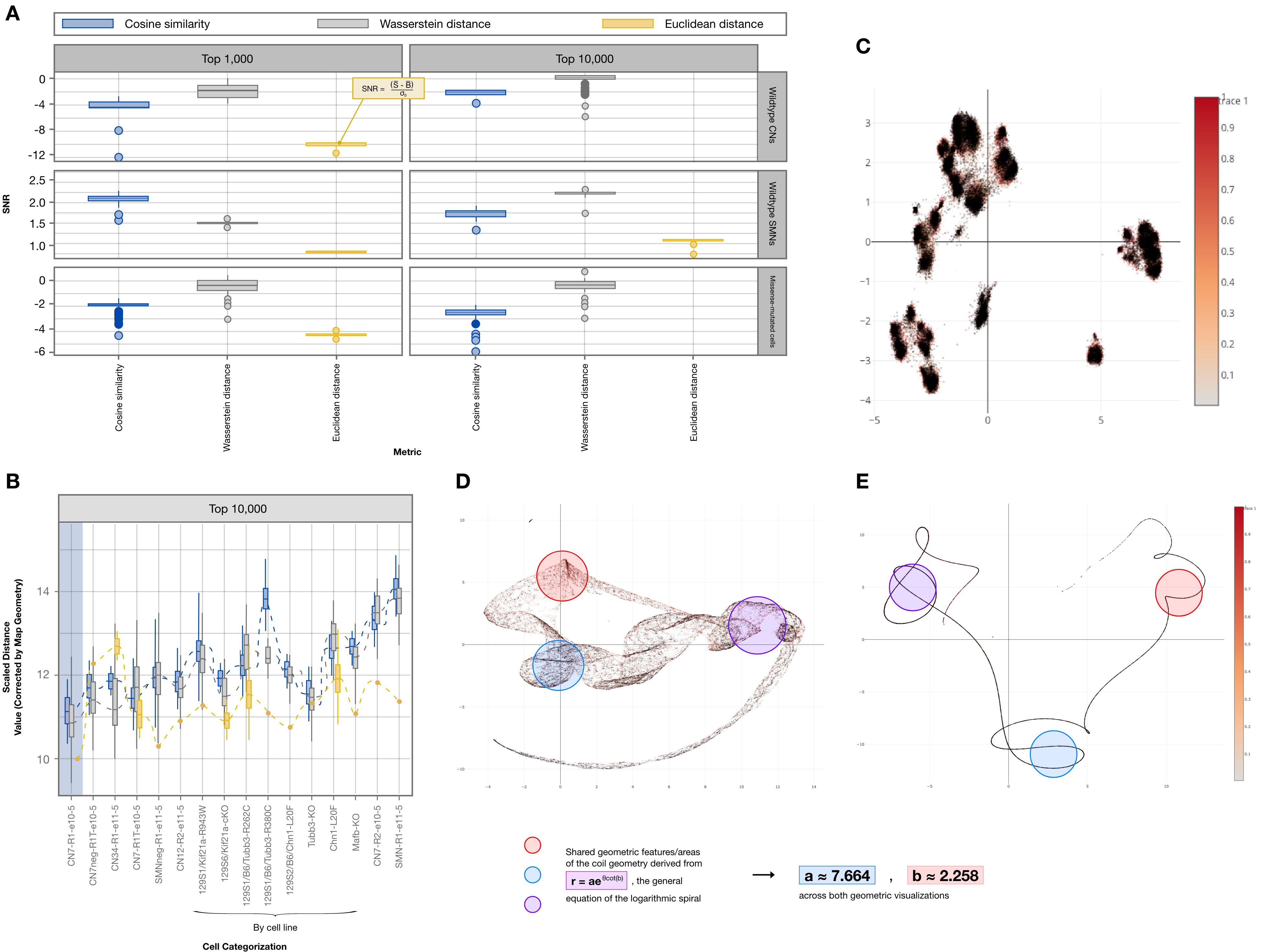
Figure 2: (A) Single-to-noise ratio boxplots yielded from the cosine similarity, Wasserstein distance, and Euclidean distance (standard metric of comparison) metrics, demonstration the statistical distribution of SNR values and overall accuracy of the elected metrics. (B) Boxplots and distributions of corrected scaled distance values for each metric. 2-D UMAP embeddings of (C) the Euclidean distance, (D) the Wasserstein distance, and (E) cosine similarity with similar features shown and the estimated coefficient values of the logarithmic spiral from which their geometries appear to be derived.

To view the topology of the metrics in 50-D such that all major cell features are reflected in the map, I complete downstream analysis with each metric to obtain the chromatin accessibility scores, then plot each chromosomal read, with TF motifs classified and displayed (Figure 3A). Appending these chromatin accessibility scores and loci of chromatin accessible peaks to the 50 major features contained within the original data, I construct UMAPs—each with distinguishing color scales—of several batches of features, overlaid within a single vector space, as only $n=5$ dimensions can be computationally visualized at once (Figure 3B).

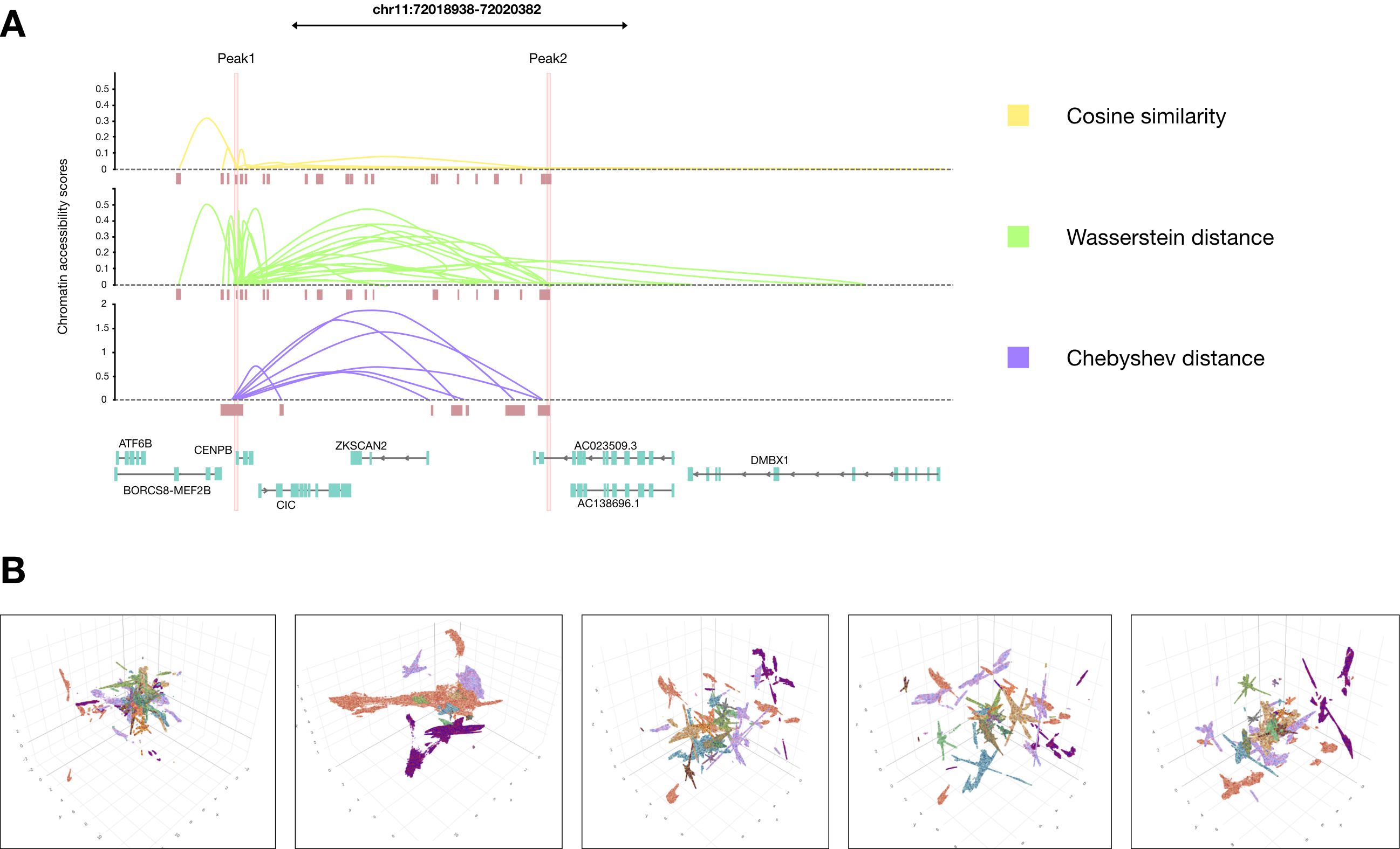
Figure 3: (A) Visualization of co (chromatin)-accessibility scores obtained using the cosine similarity, Wasserstein distance, and Chebyshev distance metrics (a standard metric for comparison). (B) 50 major dimensions of all 85,089 cell profiles divided into several color scales and graphs superimposed into one viewing window.

I perform foreground-background images on all viewing angles $\theta$ of superimposed UMAP embeddings. Following the previous computation of the SNR for the produced embeddings, I derive a mean-squared error (MSE) approximation, which serves as the function to isolate a 2-D ‘silhouette’ from a 3-D geometry:

$$\textnormal{MSE}=\frac{\sum\limits^{M-1}_{x=0}\sum\limits^{N-1}_{y=0}\left[f(x,y)-\widehat{f}(x,y)\right]^{2}}{MN}$$

From the MSE at all $\theta$, I identify and remove background patches of noise from the original image, resulting in the 2-D silhouettes (4A). These silhouettes are again superimposed to produce the global 50-D structure of the cell profiling embeddings under noise-minimized conditions. Under deformations, the cosine similarity (Figure 4B) and Wasserstein distance (Figure 4C) topologies exhibit homeomorphism to a helical structure. This topological equivalence lends to the metrics’ accuracy and precision on $M_{\textnormal{cells}}$, in which distances appear locally Euclidean, and also further demonstrates a significant correlation between $d_{\textnormal{a}}$ and $d_{\textnormal{p}}$. Additionally, when compared to the Chebyshev distance (4D), homology was not observed in the embeddings. Instead, several discontinuous spherical topologies were discovered, which indicates that, as confirmed through exhaustive tests, the other standard metrics do not fit the geometric structure of $M_{\textnormal{cells}}$ as to accurately reflect the distance or similarity between cells within an omics clustering map.

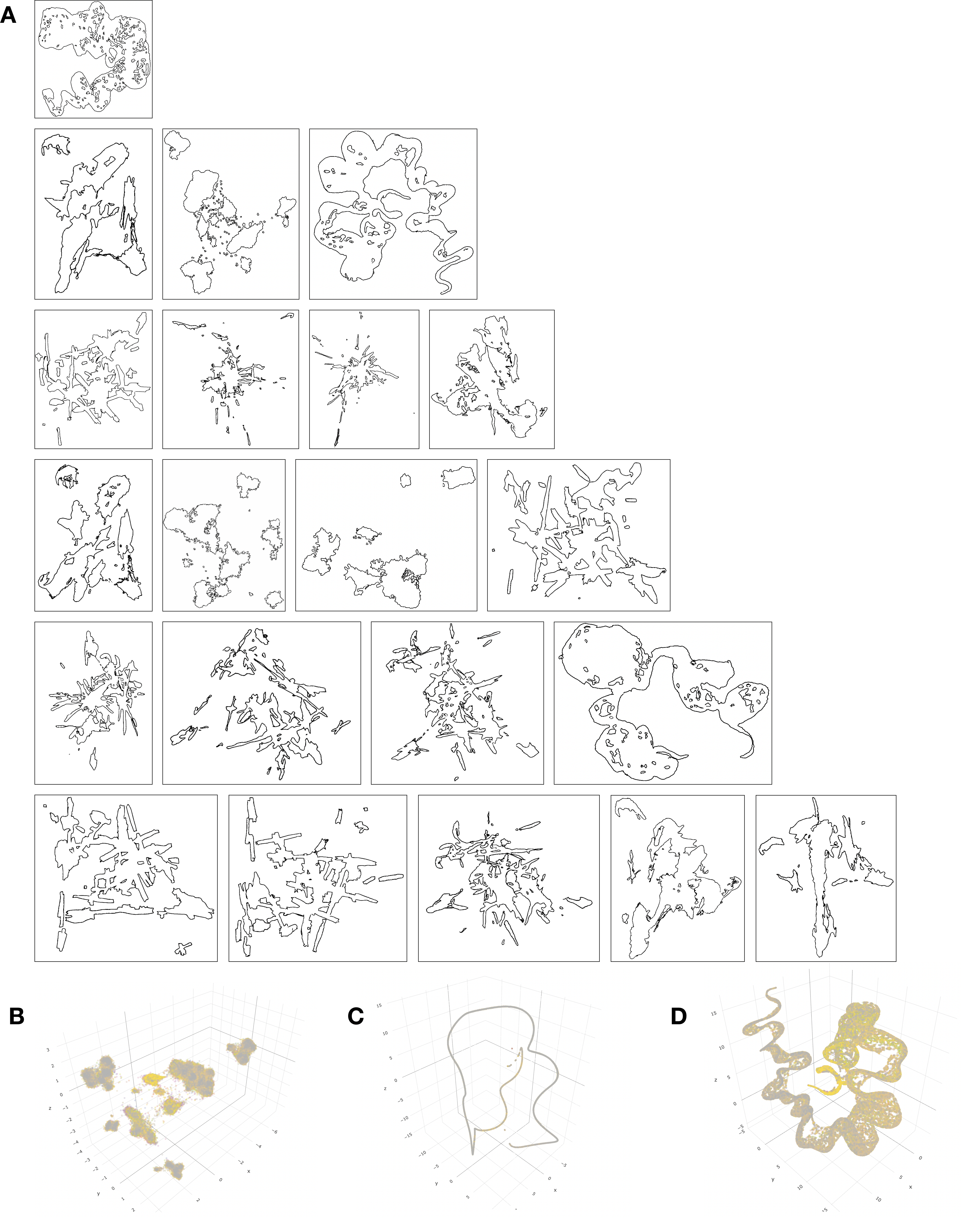
Figure 4: (A) 2-D silhouette geometries obtained via foreground-background separation using the MSE. (B) 50-D topologies within a 3-D visualization window obtained via superimposing all silhouettes from all viewing angles $\theta$.

2.3.3 An ‘Optimal’ Custom Metric Combines the Cosine Similarity and Wasserstein Distance

From the novel criterion outlined in Section 2.2, I determine and validate that the cosine similarity metric is $d_{\textnormal{a}}$ and the Wasserstein distance is $d_{\textnormal{b}}$ [54, 55, 3, 4]. The cosine similarity metric takes an input of two vectors $\vec{e}$ and $\vec{z}$ and finds $\cos(\phi)$, where $\phi$ represents the dot product of the two vectors. The cosine similarity ranges from -1 to 1, where 1 indicates that the two vectors are identical, 0 indicates that they are orthogonal, and -1 indicates that they are diametrically opposed.

The Wasserstein distance begins with probability distributions $E$ and $Z$ in $n$-dimensional space $\mathbb{R}$ over a region $D$ [56, 57]. Given that $E$ and $Z$ are represented by a set of clusters describing the cluster’s mean, I calculate the distances between these distributions by determining the cost, $d$, of transforming one distribution into the other. $E$ and $Z$ are signatures, whose minimal overall cost is a flow $\textbf{W}=\left[w_{i,j}\right]$ between the cluster representatives of $E$ and $Z$ [58]. Given $E=\{\left(e_{1},w_{e1}\right),\left(e_{2},w_{e2}\right),\ldots,\left(e_{n},w_{en}\right)\}$ and $Z=\{\left(z_{1},w_{z1}\right),\left(z_{2},w_{z2}\right),\ldots,\left(z_{m},w_{em}\right)\}$, and region $D=\left[d_{i,j}\right]$ is the ground distance between clusters, then I calculate optimal flow, where the work normalized by the total flow is the Wasserstein distance:

$$d(E,Z)=\underset{\gamma\in\prod(E,Z)}{\inf}\mathit{\mathbb{E}}_{(x,y)\sim\gamma}\left[\|x-y\|\right],$$

where $\prod(E,Z)$ is the product representing a set of all the joint distributions in which when a dimension is removed, I obtain marginal distributions $E$ and $Z$ and $d(E,Z)$ is the Wasserstein distance between the signatures $E$ and $Z$.

We start by considering two cells $x$ and $y$ on $M_{\textnormal{cells}}$, and compute the Wasserstein distance between their probability distributions and the cosine similarity of their mean vectors, capturing both the geometric relationship between the distributions and the differences in their shapes. This measures the geometric relationship between the two distributions by computing the cosine of the angle between their mean vectors. Combining the mathematical properties of $d_{\textnormal{a}}$ and $d_{\textnormal{b}}$, I compute and test a custom metric that maintains a helical root topology and optimizes for cell-cell similarity inference by distinguishing between $\oplus^{\prime}$, $\oplus$, and $\succ$ pairs. This ‘optimal’ metric $d_{\textnormal{o}}$ is defined as:

$$d_{\textnormal{o}}(x,y)=\frac{\alpha(1-\cos(\theta))+(1-\alpha)\sum\limits_{i=1}^{n}w_{i}\left[\sup\limits_{|f|L\leq 1}\left(\int{X_{i}}f(x)p_{i}(x)dx-\int_{Y_{i}}f(y)q_{i}(y)dy\right)\right]}{\alpha+(1-\alpha)\sum\limits_{i=1}^{n}w_{i}}$$

where $\theta$ is the angle between the mean vectors of $x$ and $y$, $n$ is the number of dimensions in the distributions $x$ and $y$, $p_{i}$ and $q_{i}$ are the probability density functions corresponding to the $i$-th dimension of $x$ and $y$, respectively, $X_{i}$ and $Y_{i}$ are the supports of $p_{i}$ and $q_{i}$, respectively, $f$ is a Lipschitz continuous function with constant 1, $|f|_{L}$ denotes the Lipschitz constant of the function $f$, $w_{i}$ is a weight parameter that determines the relative importance of the $i$-th dimension, and $\alpha$ is a weighting parameter that determines the relative importance of the cosine similarity and the Wasserstein distance between dimensions. This modified custom combined metric takes cross sections of each Wasserstein distance to compare the features of the probability distributions across dimensions. The weighting parameter $\alpha$ can be chosen to reflect the relative importance of the cosine similarity and the Wasserstein distance between dimensions in the given problem, while the weight parameters $w_{i}$ can be used to prioritize certain dimensions over others. The entire expression is dimensionless, enabling cross-dataset similarity scoring.

2.4 Special Cases

Though the general $d_{\textnormal{b}}$ and $d_{\textnormal{a}}$ are suspected as the Wasserstein distance and cosine similarity respectively, with the custom metric being the optimal distance calculation modality, there exist special cases in which the structure and form of the data favor the use of nonstandard metrics. Moreover, the currently elected $d_{\textnormal{a}}$ and $d_{\textnormal{b}}$ metrics may not be optimal in these rare cases. In the following, I investigate three non-canonical instances in which uncommon distance and similarity measures can or cannot be used.

2.4.1 Cosine Distance with Positive Valued Data

Although the cosine distance (defined as $1-\textnormal{cosine similarity}$) is not a true metric as it violates the triangle inequality, there are instances in which it can be used to accurately convey the distance between two points on the $M_{\textnormal{cells}}$ manifold. Given the data is completely normed to $\mathbb{R}_{>0}$, the cosine distance can be applied as a true distance metric to calculate pairwise similarity. However, the data presented in which cosine distance can replace cosine similarity as $d_{\textnormal{a}}$ are nonunique, as it transforms cosine similarity into a measure of distance, converting it to the same value scale of all other normalized distance metrics, which holds no added significance over cosine similarity.

2.4.2 Sørensen–Dice and Jaccard Statistics

Given two sets of discrete data $O$ and $M$, the Sørensen-Dice coefficient is defined as

$$d(O,M)=\frac{2|O\cap M|}{|O|+|M|},$$

where $|O|$ and $|M|$ are the cardinalities of the sets, and $|O\cap M|$ represents the number of elements shared across both sets [62, 63]. In vector form, this is represented as twice the dot product of the two vectors divided by the sum of the squares of the magnitudes of either vector. The Jaccard index is calculated similarly, with the number of the shared elements between sets no longer being doubled. Both statistics can be used to accurately determine the similarity and diversity between cells in clustering when the values of the data are normed to $[0,1]$ and of a uniform probability distribution [64, 65, 66].

To confirm the use of Sørensen–Dice and Jaccard statistics as a special case of $d_{\textnormal{a}}$ or $d_{\textnormal{b}}$, I performed distance testing in a structurally identical truncated version of our scATAC-Seq dataset whose value ranges nearly conform to a uniform distribution. Under conditions where the data was edited to fit a uniform distribution, denoted as $\mathcal{U}$, both the Sørensen–Dice and Jaccard similarity measures satisfied Proposition 2.1 and its emergent properties, achieving high-throughput distinction between $\oplus^{\prime}$ and $\oplus$ pairs, as well as highlighting significant diversity between cells of the nature $c_{\textnormal{0}}$ and $c_{1}$ in $\succ$ pairs. However, in a similarly truncated scATAC-Seq dataset of a non-uniform distribution, neither statistic behaved as $d_{\textnormal{b}}$ or $d_{\textnormal{a}}$. From this data, I conclude that on average ($\bar{\textbf{x}}$), under the condition $\mathcal{U}$, the Sørensen–Dice and Jaccard statistics act as both $d_{\textnormal{b}}$ and $d_{\textnormal{a}}$, outperforming all other general metrics and having little numerical distinction in distance values from one another.

2.4.3 Extended $p$ of Minkowski

The Minkowski distance is a generalization of other distance metrics such as Euclidean distance, Manhattan distance, and Chebyshev distance, and it is defined as:

$$d_{p}(x,y)=\left(\sum_{i=1}^{n}|x_{i}-y_{i}|^{p}\right)^{1/p}$$

where $x$ and $y$ are two $n$-dimensional vectors, and $p$ is a positive constant representing the order of the Minkowski distance. The most notable cases of the Minkowski distance orders are $p=1,2,\textnormal{and }\infty$ [67, 68, 69]. However, there are three additional cases of interest: $p=0.25,0.5,\textnormal{ and }4$, which represent different forms less or greater than the standard $p=1$ unit circle $x^{2}+y^{2}=1$. However, the calculations of these cases of Minkowski yielded no distinctive results from the Chebyshev and Manhattan distance. Each of the new cases of $p$ instead decreases adherence to the 0.02 rule described in Corollary 3. Therefore, there are no $d_{\textnormal{a}}$ or $d_{\textnormal{b}}$ cases of the Minkowski metric. I extend the improbability of the $d_{\textnormal{a}}$ and $d_{\textnormal{b}}$ identity to the classical cases of the Minkowski metric.

3 Results

3.1 Custom Metric Benchmarking

3.1.1 Criteria-Constructed Metric Outperforms Optimal Transport in Accuracy, Precision, and Utility Across All Neuronal Cell Lines

With this formally-defined metric, I perform a series of tests to demonstrate its utility over traditional metrics, particularly Optimal Transport. First, I evaluate the cohesion and separation of clusters formed metrics via silhouette scoring and c-score for the cosine similarity and Wasserstein distance. Both metrics exhibit consistently high statistical performance across varying cell distributions and rough organizations of the data (Figure 5A), confirming them as the appropriate bases for the custom metric and also demonstrating that both metrics properly cluster data.

I then compare three accuracy benchmarks from the custom metric to the standard metrics: imputation accuracy (Figure 5B), distance accuracy(Figure 5C), and clustering accuracy (Figure 5D). The high imputation accuracy indicates successful denoising and that a high proportion of true peaks were uncovered via the custom metric. Furthermore, the distance accuracy tests the calculated distance against the known ground truth distances, with a higher score, such as that of the custom metric, indicating a minimal discrepancy between the set of values. Finally, the clustering accuracy of the metric demonstrates its superiority over the standard metrics in categorizing cells within a highly homogeneous cell line based on any given feature and visualizing the omics data, again supporting that the metric detects dissimilarity between cell profiles with high fidelity. Across all cases and cell lines, the custom metric outperforms Optimal Transport and the 8 other standard metrics, on average. Furthermore, it exhibits exceptionally high performance in distance and clustering accuracy, indicating that it best reflects cell-cell similarity.

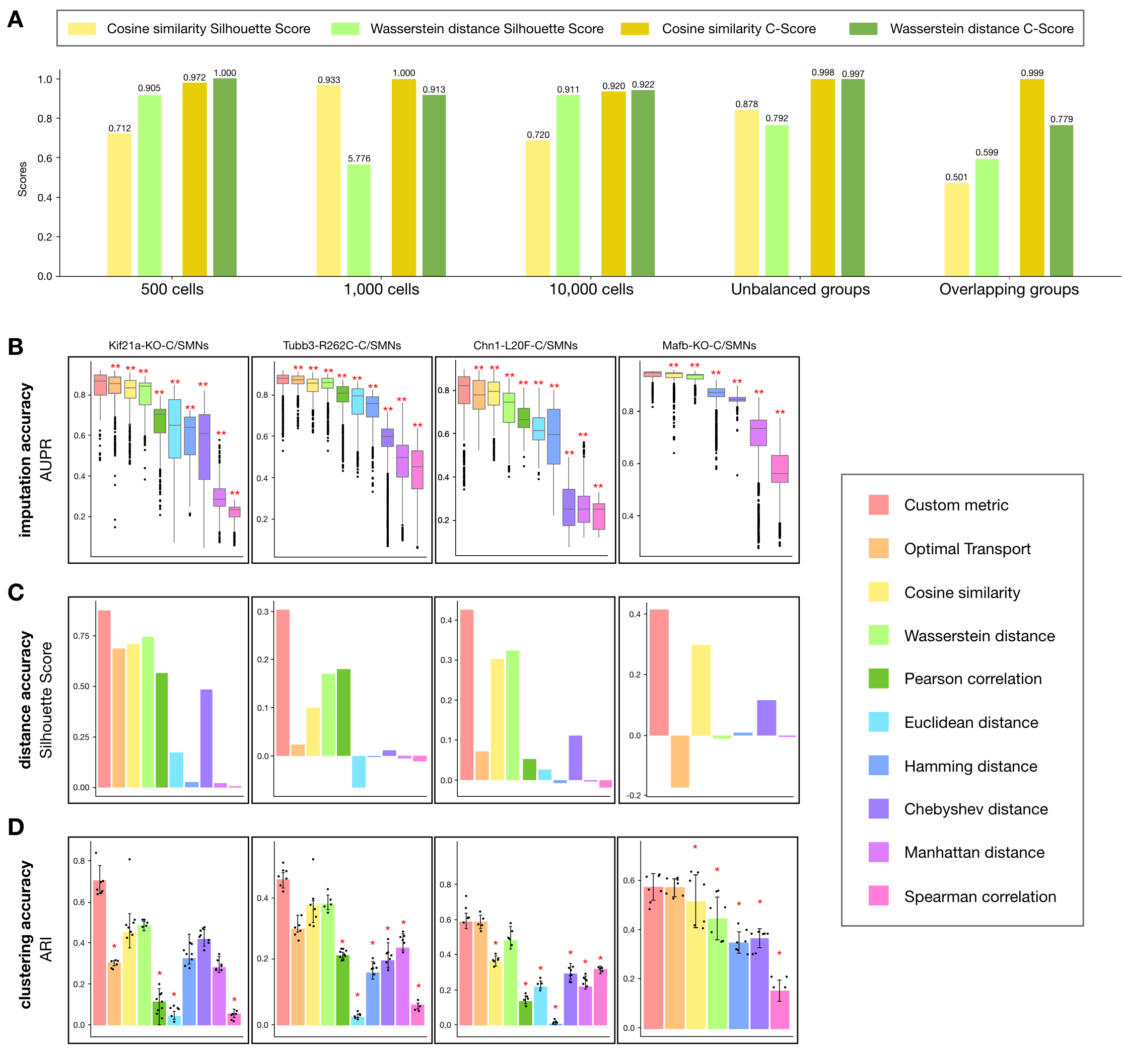
Figure 5: (A) Silhouette and c-scoring for cosine similarity and the Wasserstein distance across groupings of 500, 1000, and 10,000 cells with unbalanced groups and overlapping clusters. (B) Boxplots for imputation evaluation where the area under the precision-recall curve (AUPR) is plotted on the $y$-axis. The asterisk and the two asterisks mean that the method is outperformed by the custom metric with significance levels of 0.05 and 0.01 at a confidence level of 0.95 (Wilcoxon Rank Sum test, paired, two-sided), respectively, as in Li et al. (C) Bar graphs of the preliminary silhouette scores ($y$-axis) for the standard metrics to quantify distance accuracy. (D) Barplots to demonstrate the clustering accuracy for distinct imputation methods, where the $y$-axis indicates the mean adjusted Rand Index (ARI). The asterisk and the two asterisks mean that the method is outperformed by the top-ranked method with significance levels of 0.05 and 0.01 at a confidence level of 0.95 ($n=8$ independent clustering experiments, Wilcoxon Rank Sum test, paired, two-sided), respectively, as in Li, et al. [70]. In all plots, groupings are done based on cell line phenotypes, as indicated.

3.1.2 Criteria-Constructed Metric Outperforms Optimal Transport in Computational Complexity Across All Neuronal Cell Line Calculations

An additional, striking utility of the custom metric resulting from the selection criteria is the significant reduction in runtime needed to complete downstream analysis of omics data or to render high-dimensional embeddings. To obtain a quantitative profiling consistency across all 85,089 neurons, I construct a two-sample Fisher exact test for every generated profile, and then average results into two groupings of missense-mutated neurons (MMNs) and wildtype neurons (WTNs). A greater exactness indicates a fixed and precise value of dissimilarity regarding the identified peaks of open chromatin found $\oplus^{\prime}$ and $\oplus$ pairs, which differ significantly from that of $\succ$ pairs.

Computational analysis was completed on a 10-core Precision 7920 Tower Workstation Dell Supercomputer. The custom metric exhibits a greater average Fisher coefficient over mutated
($\sim 0.715$) and non-mutated cells ($\sim 0.573$), and an overall shorter average runtime for all features (18.9 minutes) with a two-sided $t$-test producing $p=0.00141$, indicating that the computational efficiency of the custom metric is significantly greater compared to Optimal Transport (Table 1). This is likely a result of the mathematical properties of the custom metric combining that of a proximity metric, Wasserstein, and similarity metric, cosine, which reduces the overall computational complexity of the omics analysis protocol by utilizing a metric that is highly fitted to the data. This further enhances the utility of both the distance selection criteria and custom metric.

Table 1: Computational Performance of the Custom Metric versus Optimal Transport

Custom Metric Optimal Transport MMNs    MMN expression    MMN peak ID    MMN average 0.771 0.658 0.715 0.472 0.611 0.541 WTNs    WTN characterization    WTN peak ID    WTN average 0.617 0.529 0.573 0.593 0.400 0.497 All-cell average 0.644 0.519 Runtime 18.9 minutes 241.5 minutes

3.2 Custom Metric Experimental Performance

3.2.1 Custom Metric Reveals Putative Novel Spinal and Cranial Motor Neuron Subpopulations

Downstream cluster analysis recapitulated several known clusters of neurons within the ATAC-Seq dataset and also yielded findings from novel cell populations. In particular, I identified putative CN3 and CN7 cranial nerves from the cluster identities (Figure 6A), as well as SMN32 and SMN20 spinal nerves. We then mapped these nerves, which had been maldeveloped in the non-wildtype mice, in vivo (Figure 6B, 6C). 16 other currently unexplored TF motifs and neuron subclusters were also identified. These areas exhibited unusual cis-regulatory activity, as their chromatin accessibility profiles possessed a $z$-score of 5.6 standard deviations from the mean value. Such a deviation would not be detected by traditional standard metrics; the improvements presented by the criteria and elected distance metrics to augment the empirical data qualities.

3.2.2 Putative Loci of Noncoding Mendelian Mutations in CCDD-Afflicted Neurons Discovered

The exome, or genetic regions that do not code for proteins, comprises nearly 99% of the human genome [71, 72]. Given its vastly increased search space, it has previously been difficult to pinpoint the areas on the genome at which mutations such as those responsible for CCDDs are located [73]. The custom metric was able to identify 18 potential areas where mutations may have occurred due to an altered presence of heterochromatin in such locations and nominate 3 specific developmental enhancers in underdeveloped cranial neurons (Figure 6D).

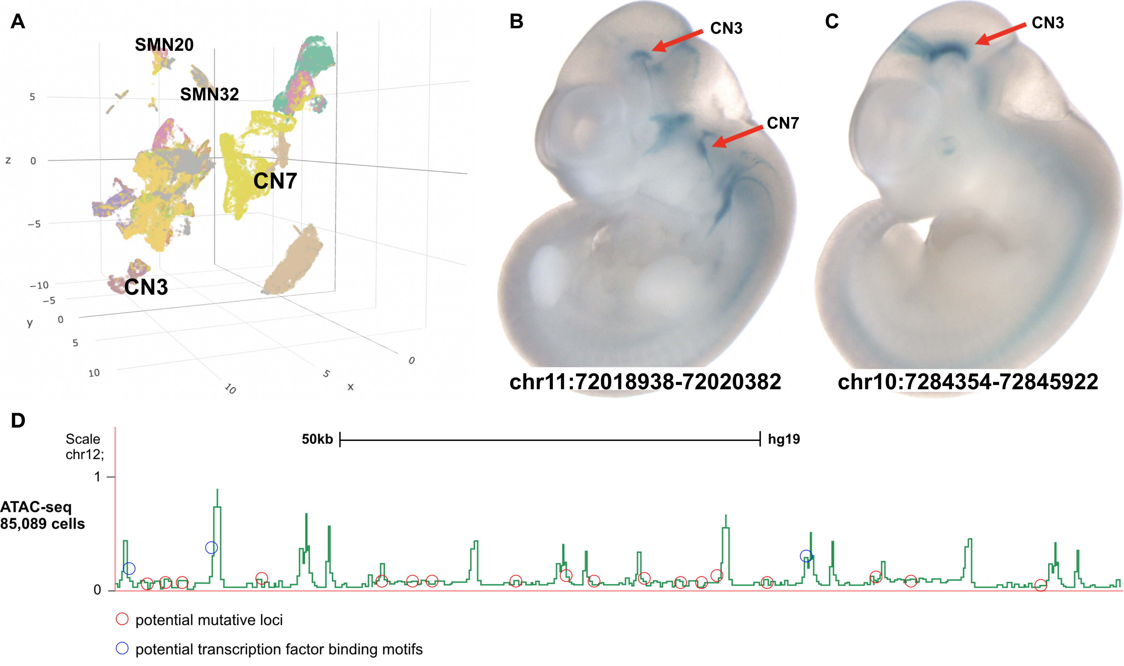
Figure 6: (A) Three-dimensional UMAP embedding of 85,089 high-quality single-cell chromatin accessibility profiles using the custom metric from dissected cranial motor neurons. Cells are colored by cluster identity. 35 Clusters corresponding to putative cranial nerves CN3, SMN20, SMN32, and CN7 are labelled. (B, C) LacZ in vivo enhancer assay validation for candidate enhancers ascertained by single-cell ATAC-seq in cranial motor neurons specific to B, CN3 and CN7, and C, CN3 only. (D) Chromatin accessibility profile yielded from novel KIF21A missense strains sampled from the larger dataset, with potentially mutative loci and TF motifs identified.

Using in vivo reporter constructs, we microdissected, collected, and FACS-purified approximately 500,000 developing cranial motor neurons 3, 4, 6, 7, 12, spinal motor neurons, and green fluorescent protein-negative non-motor neuron control cells. Using downstream analysis techniques via the custom distance metrics, novel spinal and cranial motor neuron candidates, including their embryonic locations (Figure 6B, 6C) and chromosomal homology (Figure 6A), were discovered.

4 Discussion

Single cell-omics technologies have emerged as the premiere method to analyze the biological features of cells in large batches. With the decrease of cost per human genome over time surpassing that of Moore’s law, the abundance of single-cell omics, multi-omics, and other sequencing datasets will continue to expand [74, 75, 76, 77]. As such, it is increasingly vital that more effective downstream analysis methods are employed to better reflect global heterogeneity for cellular classification, developmental, and epigenetic research [78, 79]. As such, identifying and developing optimal distance metrics, and the determinants of the quality of these molecular markers is paramount.

This study pioneers a generalized criterion to elect distance metrics for omics analysis, the basis of which is a proven hierarchy of distance (Proposition 2.1). I evaluate the discrepancies with the hierarchical order of the distances between cells of certain pairs (Corollary 1), define the precision and accuracy of distance measures in metric space (Corollary 2), establish a means of evaluating statistical significance and discerning between cell pair distances (Corollary 3), and describe geometric and topological properties that extend as the dimensions of the cell profiles are further persevered (Corollary 4, 5). The criterion yields two generally accurate and robust measures, the Wasserstein distance and cosine similarity. Through first principles, it was expected that a non-Minkowski metric would be the best performing in complex environments such as clustering, where linear calculations of distance become increasingly obsolete, ultimately determining cosine similarity as $d_{\textnormal{a}}$ and Wasserstein distance as $d_{\textnormal{p}}$. I develop an ‘optimal’ custom distance metric that combines properties of $d_{\textnormal{a}}$ and $d_{\textnormal{p}}$ that successfully identify neuron subclusters and assess regulatory sites within the genome to identify de novo Mendelian KIF21A mutations in CCDDs within the scATAC-Seq test data. Finally, I also identify a special case in which the Jaccard and Sørensen-Dice metrics become the most accurate metrics. I hope to identify additional cases in the future, such as utilizing quasimetrics and semimetrics, and scale the findings from these results to non-binarized-normed data, such as ChIP-Seq and post-integration RNA-Seq [80, 81].

The performance of the criterion and nominated distance metrics suggest that they can be used in a variety of cases, such as in cellular biology and pharmacogenetics. The criterion is also method-blind, solely optimizing for distance, so it can be adapted to fit any set of analyzable biological characteristics. As demonstrated by preliminaries in neuronal scATAC-Seq datasets, this novel method enhances pathogenic and genetic findings from single-cell omics, offering computational speedups and more accurate and precise data.

References

- [1] H. Chen, C. Lareau, T. Andreani, M. E. Vinyard, S. P. Garcia, K. Clement, M. A. Andrade-Navarro, J. D. Buenrostro, and L. Pinello. Assessment of computational methods for the analysis of single-cell atac-Seq data. Genome Biology, 20(1):241, Nov 2019.
- [2] L. McInnes, J. Healy, and J. Melville. UMAP: Uniform manifold approximation and projection for dimension reduction, 2018.
- [3] K. Zhang, J. D. Hocker, M. Miller, X. Hou, J. Chiou, O. B. Poirion, Y. Qiu, Y. E. Li, K. J. Gaulton, A. Wang, S. Preissl, and B. Ren. A single-cell atlas of chromatin accessibility in the human genome. Cell, 184(24):5985–6001.e19, Nov. 2021.
- [4] T. N. Turner and E. E. Eichler. The role of de novo noncoding regulatory mutations in neurodevelopmental disorders. Trends in Neurosciences, 42(2):115–127, Feb. 2019.
- [5] S. S. Dey, L. Kester, B. Spanjaard, M. Bienko, and A. van Oudenaarden. Integrated genome and transcriptome sequencing of the same cell. Nature Biotechnology, 33(3):285–289, Mar 2015.
- [6] J. Beal. Signal-to-noise ratio measures efficacy of biological computing devices and circuits. Front. Bioeng. Biotechnol., 3:93, June 2015.
- [7] S. J. Clark, R. Argelaguet, C.-A. Kapourani, T. M. Stubbs, H. J. Lee, C. Alda-Catalinas, F. Krueger, G. Sanguinetti, G. Kelsey, J. C. Marioni, O. Stegle, and W. Reik. scNMT-Seq enables joint profiling of chromatin accessibility dna methylation and transcription in single cells. Nature Communications, 9(1):781, Feb 2018.
- [8] D. Jovic, X. Liang, H. Zeng, L. Lin, F. Xu, and Y. Luo. Single-cell RNA sequencing technologies and applications: A brief overview. Clinical and Translational Medicine, 12(3):e694, 2022.
- [9] B. Hwang, J. H. Lee, and D. Bang. Single-cell rna sequencing technologies and bioinformaticspipelines. Experimental & Molecular Medicine, 50(8):1–14, Aug 2018.
- [10] J. Han, M. Kamber, and J. Pei. 2 - getting to know your data. In J. Han, M. Kamber, and J. Pei, editors, Data Mining (Third Edition), The Morgan Kaufmann Series in Data Management Systems, pages 39–82. Morgan Kaufmann, Boston, third edition edition, 2012.
- [11] T. Wigren. The cauchy-schwarz inequality: Proofs and applications in various spaces. Faculty of Technology and Science, 2015.
- [12] N. T. Gupta, K. D. Adams, A. W. Briggs, S. C. Timberlake, F. Vigneault, and S. H. Kleinstein. Hierarchical Clustering Can Identify B Cell Clones with High Confidence in Ig Repertoire Sequencing Data. J Immunol, 198(6):2489–2499, 03 2017.
- [13] R. Xiang, W. Wang, L. Yang, S. Wang, C. Xu, and X. Chen. A comparison for dimensionality reduction methods of single-cell RNA-seq data. Frontiers in Genetics, 12, 2021.
- [14] D. Sinwar and R. Kaushik. Study of euclidean and manhattan distance metrics using simple k-means clustering. 2, 05 2014.
- [15] F. Nielsen. Computational Information Geometry: Pursuing the Meaning of Distances, pages 258–261. 11 2010.
- [16] J. Bennett, M. Pomaznoy, A. Singhania, and B. Peters. A metric for evaluating biological information in gene sets and its application to identify co-expressed gene clusters in pbmc. PLOS Computational Biology, 17(10):1–18, 10 2021.
- [17] C. N. Heiser and K. S. Lau. A quantitative framework for evaluating single-cell data structure preservation by dimensionality reduction techniques. Cell Reports, 31(5):107576, 2020.
- [18] P. A. Jaskowiak, R. J. Campello, and I. G. Costa. On the selection of appropriate distances for gene expression data clustering. BMC Bioinformatics, 15(2):S2, Jan 2014.
- [19] B. Nguyen, P. Rubbens, F.-M. Kerckhof, N. Boon, B. De Baets, and W. Waegeman. Learning single-cell distances from cytometry data. Cytometry Part A, 95, 05 2019.
- [20] A. Satpathy, J. Granja, K. Yost, Y. Qi, F. Meschi, G. Mcdermott, B. Olsen, M. Mumbach, S. Pierce, M. Corces, P. Shah, J. Bell, D. Jhutty, C. Nemec, J. Wang, L. Wang, Y. Yin, P. Giresi, A. Chang, and H. Chang. Massively parallel single-cell chromatin landscapes of human immune cell development and intratumoral t cell exhaustion. Nature Biotechnology, 37:1, 08 2019.
- [21] J. M. Shinwari, A. Khan, S. Awad, Z. Shinwari, A. Alaiya, M. Alanazi, A. Tahir, C. Poizat, and N. A. Tassan. Recessive mutations in COL25a1 are a cause of congenital cranial dysinnervation disorder. The American Journal of Human Genetics, 96(1):147–152, jan 2015.
- [22] R. Singh, B. L. Hie, A. Narayan, and B. Berger. Schema: metric learning enables interpretable synthesis of heterogeneous single-cell modalities. Genome Biology, 22(1), may 2021.
- [23] J. Shlens. Notes on kullback-leibler divergence and likelihood, 2014.
- [24] D. A. Cusanovich, A. J. Hill, D. Aghamirzaie, R. M. Daza, H. A. Pliner, J. B. Berletch, G. N. Filippova, X. Huang, L. Christiansen, W. S. DeWitt, C. Lee, S. G. Regalado, D. F. Read, F. J. Steemers, C. M. Disteche, C. Trapnell, and J. Shendure. A single-cell atlas of In-Vivo mammalian chromatin accessibility. Cell, 174(5):1309–1324.e18, Aug 2018.
- [25] G.-J. Huizing, G. Peyré, and L. Cantini. Optimal transport improves cell–cell similarity inference in single-cell omics data. Bioinformatics, 38(8):2169–2177, Apr 2022.
- [26] C. S. Punla, https://orcid.org/ 0000-0002-1094-0018, cspunla@bpsu.edu.ph, R. C. Farro, https://orcid.org/0000-0002-3571-2716, rcfarro@bpsu.edu.ph, and Bataan Peninsula State University Dinalupihan, Bataan, Philippines. Are we there yet?: An analysis of the competencies of BEED graduates of BPSU-DC. International Multidisciplinary Research Journal, 4(3):50–59, Sept. 2022.
- [27] R. Fang, S. Preissl, Y. Li, X. Hou, J. Lucero, X. Wang, A. Motamedi, A. K. Shiau, X. Zhou, F. Xie, E. A. Mukamel, K. Zhang, Y. Zhang, M. M. Behrens, J. R. Ecker, and B. Ren. Comprehensive analysis of single cell ATAC-seq data with SnapATAC. Nature Communications, 12(1), feb 2021.
- [28] V. Rai, D. X. Quang, M. R. Erdos, D. A. Cusanovich, R. M. Daza, N. Narisu, L. S. Zou, J. P. Didion, Y. Guan, J. Shendure, S. C. Parker, and F. S. Collins. Single-cell atac-seq in human pancreatic islets and deep learning upscaling of rare cells reveals cell-specific type 2 diabetes regulatory signatures. Molecular Metabolism, 32:109–121, 2020.
- [29] K. Sahinyan, D. M. Blackburn, M.-M. Simon, F. Lazure, T. Kwan, G. Bourque, and V. D. Soleimani. Application of ATAC-seq for genome-wide analysis of the chromatin state at single myofiber resolution. eLife, 11, feb 2022.
- [30] N. Adossa, S. Khan, K. T. Rytkönen, and L. L. Elo. Computational strategies for single-cell multi-omics integration. Computational and Structural Biotechnology Journal, 19:2588–2596, 2021.
- [31] W. Koh and S. Hoon. MapCell: Learning a comparative cell type distance metric with siamese neural nets with applications toward cell-type identification across experimental datasets. Frontiers in Cell and Developmental Biology, 9, nov 2021.
- [32] X. Dai and L. Shen. Advances and trends in omics technology development. Frontiers in Medicine, 9, jul 2022.
- [33] A. Thibodeau, A. Eroglu, C. S. McGinnis, N. Lawlor, D. Nehar-Belaid, R. Kursawe, R. Marches, D. N. Conrad, G. A. Kuchel, Z. J. Gartner, J. Banchereau, M. L. Stitzel, A. E. Cicek, and D. Ucar. AMULET: a novel read count-based method for effective multiplet detection from single nucleus ATAC-seq data. Genome Biology, 22(1), sep 2021.
- [34] F. Yan, D. R. Powell, D. J. Curtis, and N. C. Wong. From reads to insight: a hitchhiker’s guide to ATAC-seq data analysis. Genome Biology, 21(1), feb 2020.
- [35] J. Ding and A. Regev. Deep generative model embedding of single-cell RNA-seq profiles on hyperspheres and hyperbolic spaces. Nature Communications, 12(1):2554, May 2021.
- [36] J. M. Lee. Topological Spaces, pages 19–48. Springer New York, New York, NY, 2011.
- [37] S. Cai, G. K. Georgakilas, J. L. Johnson, and G. Vahedi. A cosine similarity-based method to infer variability of chromatin accessibility at the single-cell level. Frontiers in Genetics, 9, 2018.
- [38] V. Huynh, N. Ho, N. Dam, X. Nguyen, M. Yurochkin, H. Bui, and D. Phung. On efficient multilevel clustering via wasserstein distances. 2019.
- [39] A. Hamza and A. Jehad. Assessment of hamming distance and self organization map in solving cell formation problem. IOP Conference Series: Materials Science and Engineering, 671:012025, 01 2020.
- [40] J. Žurauskiene and C. Yau. pcareduce: Hierarchical clustering of single cell transcriptional profiles. bioRxiv, 2015.
- [41] E. R. Watson, A. Mora, A. T. Fard, and J. C. Mar. How does the structure of data impact cell–cell similarity? evaluating how structural properties influence the performance of proximity metrics in single cell RNA-seq data. Briefings in Bioinformatics, sep 2022.
- [42] H. Han, T. Zhang, C. Li, M. L. Benton, J. Wang, and J. Li. Explainable -SNE for single-cell RNA-seq data analysis. bioRxiv, 2022.
- [43] S. M. Zandavi, F. C. Koch, A. Vijayan, F. Zanini, F. V. Mora, D. G. Ortega, and F. Vafaee. Disentangling single-cell omics representation with a power spectral density-based feature extraction. Nucleic Acids Research, 50(10):5482–5492, may 2022.
- [44] Y. Wang, H. Huang, C. Rudin, and Y. Shaposhnik. Understanding how dimension reduction tools work: An empirical approach to deciphering -SNE, UMAP, triMAP, and paCMAP for data visualization. 2020.
- [45] L. Pellis, N. L. W. F. van Hal, J. Burema, and J. Keijer. The intraclass correlation coefficient applied for evaluation of data correction, labeling methods, and rectal biopsy sampling in DNA microarray experiments. Physiological Genomics, 16(1):99–106, dec 2003.
- [46] H. Yuan and D. R. Kelley. scBasset: sequence-based modeling of single-cell ATAC-seq using convolutional neural networks. Nature Methods, 19(9):1088–1096, aug 2022.
- [47] Y. Hu, Q. An, K. Sheu, B. Trejo, S. Fan, and Y. Guo. Single cell multi-omics technology: Methodology and application. Frontiers in Cell and Developmental Biology, 6, apr 2018.
- [48] G. Misevic. Single-cell omics analyses with single molecular detection: challenges and perspectives. The Journal of Biomedical Research, 35(4):264, 2021.
- [49] Q. Yuan and Z. Duren. Integration of single-cell multi-omics data by regression analysis on unpaired observations. Genome Biology, 23(1), jul 2022.
- [50] T. M. Weiskittel, C. Correia, G. T. Yu, C. Y. Ung, S. H. Kaufmann, D. D. Billadeau, and H. Li. The trifecta of single-cell, systems-biology, and machine-learning approaches. Genes, 12(7), 2021.
- [51] A. Wehling, D. Loeffler, Y. Zhang, T. Kull, C. Donato, B. Szczerba, G. C. Ortega, M. Lee, A. Moor, B. Göttgens, N. Aceto, and T. Schroeder. Combining single-cell tracking and omics improves blood stem cell fate regulator identification. Blood, 140(13):1482–1495, sep 2022.
- [52] R. Bellazzi, A. Codegoni, S. Gualandi, G. Nicora, and E. Vercesi. The gene mover’s distance: Single-cell similarity via optimal transport, 2021.
- [53] R. C. Gonzalez and R. E. Woods. Digital image processing. 2018.
- [54] M. C. Whitman and E. C. Engle. Ocular congenital cranial dysinnervation disorders (CCDDs): insights into axon growth and guidance. Human Molecular Genetics, 26(R1):R37–R44, Apr. 2017.
- [55] E. C. Engle. Oculomotility disorders arising from disruptions in brainstem motor neuron development. Archives of Neurology, 64(5):633, May 2007.
- [56] K. Cao, Y. Hong, and L. Wan. Manifold alignment for heterogeneous single-cell multi-omics data integration using pamona. Bioinformatics, 38(1):211–219, Aug. 2021.
- [57] A. J. Tarashansky, Y. Xue, P. Li, S. R. Quake, and B. Wang. Self-assembling manifolds in single-cell RNA sequencing data. eLife, 8, Sept. 2019.
- [58] Z. He, A. Brazovskaja, S. Ebert, J. G. Camp, and B. Treutlein. CSS: cluster similarity spectrum integration of single-cell genomics data. Genome Biology, 21(1), Sept. 2020.
- [59] L. Alessandri, M. L. Ratto, S. G. Contaldo, M. Beccuti, F. Cordero, M. Arigoni, and R. A. Calogero. Sparsely connected autoencoders: A multi-purpose tool for single cell omics analysis. International Journal of Molecular Sciences, 22(23):12755, Nov. 2021.
- [60] P. Yang, H. Huang, and C. Liu. Feature selection revisited in the single-cell era. Genome Biology, 22(1), Dec. 2021.
- [61] S. Ogbeide, F. Giannese, L. Mincarelli, and I. C. Macaulay. Into the multiverse: advances in single-cell multiomic profiling. Trends in Genetics, 38(8):831–843, Aug. 2022.
- [62] A. Mcloughlin and H. Huang. Shared differential expression-based distance reflects global cell type relationships in single-cell RNA sequencing data. Journal of Computational Biology, 29(8):867–879, aug 2022.
- [63] M. D. Luecken and F. J. Theis. Current best practices in single-cell RNA-seq analysis: a tutorial. Molecular Systems Biology, 15(6), jun 2019.
- [64] M. J. T. Stubbington, O. Rozenblatt-Rosen, A. Regev, and S. A. Teichmann. Single-cell transcriptomics to explore the immune system in health and disease. Science, 358(6359):58–63, oct 2017.
- [65] C. S. Punla, https://orcid.org/ 0000-0002-1094-0018, cspunla@bpsu.edu.ph, R. C. Farro, https://orcid.org/0000-0002-3571-2716, rcfarro@bpsu.edu.ph, and Bataan Peninsula State University Dinalupihan, Bataan, Philippines. Are we there yet?: An analysis of the competencies of BEED graduates of BPSU-DC. International Multidisciplinary Research Journal, 4(3):50–59, Sept. 2022.
- [66] M. Litviňuková, C. Talavera-López, H. Maatz, D. Reichart, C. L. Worth, E. L. Lindberg, M. Kanda, K. Polanski, M. Heinig, M. Lee, E. R. Nadelmann, K. Roberts, L. Tuck, E. S. Fasouli, D. M. DeLaughter, B. McDonough, H. Wakimoto, J. M. Gorham, S. Samari, K. T. Mahbubani, K. Saeb-Parsy, G. Patone, J. J. Boyle, H. Zhang, H. Zhang, A. Viveiros, G. Y. Oudit, O. A. Bayraktar, J. G. Seidman, C. E. Seidman, M. Noseda, N. Hubner, and S. A. Teichmann. Cells of the adult human heart. Nature, 588(7838):466–472, Sept. 2020.
- [67] Q. Shen and S. Zhang. Approximate distance correlation for selecting highly interrelated genes across datasets. PLOS Computational Biology, 17(11):e1009548, Nov. 2021.
- [68] Y. Imoto, T. Nakamura, E. G. Escolar, M. Yoshiwaki, Y. Kojima, Y. Yabuta, Y. Katou, T. Yamamoto, Y. Hiraoka, and M. Saitou. Resolution of the curse of dimensionality in single-cell RNA sequencing data analysis. Life Science Alliance, 5(12):e202201591, Aug. 2022.
- [69] L. Huo, J. J. Li, L. Chen, Z. Yu, G. Hutvagner, and J. Li. Single-cell multi-omics sequencing: application trends, COVID-19, data analysis issues and prospects. Briefings in Bioinformatics, 22(6), June 2021.
- [70] Z. Li, C. Kuppe, S. Ziegler, M. Cheng, N. Kabgani, S. Menzel, M. Zenke, R. Kramann, and I. G. Costa. Chromatin-accessibility estimation from single-cell atac-seq data with scopen. Nature Communications, 12(1):6386, Nov 2021.
- [71] M. Blencowe, D. Arneson, J. Ding, Y.-W. Chen, Z. Saleem, and X. Yang. Network modeling of single-cell omics data: challenges, opportunities, and progresses. Emerging Topics in Life Sciences, 3(4):379–398, July 2019.
- [72] A. Adil, V. Kumar, A. T. Jan, and M. Asger. Single-cell transcriptomics: Current methods and challenges in data acquisition and analysis. Frontiers in Neuroscience, 15, Apr. 2021.
- [73] C. Maniatis, C. A. Vallejos, and G. Sanguinetti. SCRaPL: A bayesian hierarchical framework for detecting technical associates in single cell multiomics data. PLOS Computational Biology, 18(6):e1010163, June 2022.
- [74] E. M. Johnson, W. Kath, and M. Mani. EMBEDR: Distinguishing signal from noise in single-cell omics data. Patterns, 3(3):100443, Mar. 2022.
- [75] G. Guo, M. Huss, G. Q. Tong, C. Wang, L. L. Sun, N. D. Clarke, and P. Robson. Resolution of cell fate decisions revealed by single-cell gene expression analysis from zygote to blastocyst. Developmental Cell, 18(4):675–685, Apr. 2010.
- [76] P. Dalerba, T. Kalisky, D. Sahoo, P. S. Rajendran, M. E. Rothenberg, A. A. Leyrat, S. Sim, J. Okamoto, D. M. Johnston, D. Qian, M. Zabala, J. Bueno, N. F. Neff, J. Wang, A. A. Shelton, B. Visser, S. Hisamori, Y. Shimono, M. van de Wetering, H. Clevers, M. F. Clarke, and S. R. Quake. Single-cell dissection of transcriptional heterogeneity in human colon tumors. Nature Biotechnology, 29(12):1120–1127, Nov. 2011.
- [77] S. Dasgupta, G. D. Bader, and S. Goyal. Single-cell RNA sequencing: A new window into cell scale dynamics. Biophysical Journal, 115(3):429–435, Aug. 2018.
- [78] C. Hafemeister and R. Satija. Normalization and variance stabilization of single-cell RNA-seq data using regularized negative binomial regression. Genome Biology, 20(1), Dec. 2019.
- [79] C. Sheng, R. Lopes, G. Li, S. Schuierer, A. Waldt, R. Cuttat, S. Dimitrieva, A. Kauffmann, E. Durand, G. G. Galli, G. Roma, and A. de Weck. Probabilistic machine learning ensures accurate ambient denoising in droplet-based single-cell omics. Jan. 2022.
- [80] R. S. Ziffra, C. N. Kim, J. M. Ross, A. Wilfert, T. N. Turner, M. Haeussler, A. M. Casella, P. F. Przytycki, K. C. Keough, D. Shin, D. Bogdanoff, A. Kreimer, K. S. Pollard, S. A. Ament, E. E. Eichler, N. Ahituv, and T. J. Nowakowski. Single-cell epigenomics reveals mechanisms of human cortical development. Nature, 598(7879):205–213, Oct. 2021.
- [81] W. Xu, W. Yang, Y. Zhang, Y. Chen, N. Hong, Q. Zhang, X. Wang, Y. Hu, K. Song, W. Jin, and X. Chen. ISSAAC-seq enables sensitive and flexible multimodal profiling of chromatin accessibility and gene expression in single cells. Nature Methods, 19(10):1243–1249, Sept. 2022.