A multiwavelength light curve analysis of the classical nova YZ Ret:
An extension of the universal decline law to the nebular phase

Abstract

YZ Ret is the first X-ray flash detected classical nova, and is also well observed in optical, X-ray, and gamma-ray. We propose a comprehensive model that explains the observational properties. The white dwarf mass is determined to be $\sim 1.33~{}M_{\sun}$ that reproduces the multiwavelength light curves of YZ Ret, from optical, X-ray, and to gamma-ray. We show that a shock is naturally generated far outside the photosphere because winds collide with themselves. The derived lifetime of the shock explains some of the temporal variations of emission lines. The shocked shell significantly contributes to the optical flux in the nebular phase. The decline trend of shell emission in the nebular phase is close to $\propto t^{-1.75}$ and the same as the universal decline law of classical novae, where $t$ is the time from the outburst.

1 Introduction

A classical nova is an explosion of hydrogen-rich envelope on a mass-accreting white dwarf (WD), which is triggered by unstable hydrogen shell-burning (see, e.g., Kato et al., 2022a, for a recent fully self-consistent nova model). The classical nova YZ Ret went into outburst in 2020. It is characterized by the first detection of an X-ray flash in classical novae (König et al., 2022; Kato et al., 2022b). GeV gamma-rays were observed during ten days just after the optical maximum, which indicates a formation of a strong shock (Sokolovsky et al., 2022). The shocked shell outside the photosphere plays an essential role in the gamma-ray emission (see, e.g., Chomiuk et al., 2021, for a recent review). X-rays are also detected from 10 days after the outburst (Sokolovsky et al., 2022). YZ Ret was also observed with longer wavelengths such as optical, infrared, and radio. In the present paper, we clarify the nature of YZ Ret by modeling the multiwavelength light curves of YZ Ret, especially, in optical, X-ray, and gamma-ray light curves in the decay phase of the nova.

In what follows, we describe the characteristic properties of the classical nova YZ Ret as well as a common evolution of a nova outburst. We also establish the temporal variations of optical fluxes from the shocked shell and show that the flux in the nebular phase follows the same trend of $L_{\rm opt,shell}\propto t^{-1.75}$ as that of the universal decline law of classical nova (Hachisu & Kato, 2006). This extension of the $L\propto t^{-1.75}$ law to the nebular phase can explain the decay trends of other classical novae.

This paper is organized as follows. First we summarize the multiwavelength observations of YZ Ret in Section 2. Section 3 describes our light curve fitting with YZ Ret. Emissions from a shocked shell are studied separately in Section 4. We propose an optical decline law of $L_{\rm opt,shell}\propto t^{-1.75}$ in the nebular phase and apply this law to various novae in Section 5. Conclusions follow in Section 6. In Appendices A and B, we summarize our basic nova model and present our light curve model, respectively.

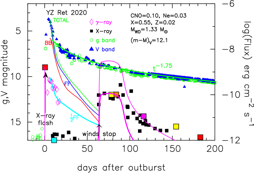
Figure 1: Multiwavelength light curves of the YZ Ret 2020 outburst. Optical $V$ (filled blue triangles) and $g$ (open green circles) magnitudes are taken from König et al. (2022). X-ray fluxes (filled black squares by Swift, filled red squares by eROSITA, filled cyan square by NuSTAR, filled orange square by NICER, filled yellow squares by XMM-Newton, filled magenta square by Chandra). Gamma-ray fluxes (open magenta diamonds by Fermi/LAT). The origin of time is set to be $t_{0}=$ UT 2020 July 7, 16:47:20 $=$ JD 2,459,038.19954 $=$ MJD 59,037.69954, which marks the first detection of YZ Ret in outburst. Solid lines show our best fit model of a 1.33 $M_{\sun}$ WD (Ne2). The red line labeled BB is the $V$ magnitude calculated by a blackbody approximation of the model photosphere. The blue line (FF) is the $V$ magnitude from free-free emission of the wind. The thin green line (TOTAL) is the sum of BB and FF fluxes. These $V$ light curves are shown from near optical $V$ maximum to the end of the wind. The thick green line labeled $t^{-1.75}$ shows an approximated $V$ magnitude model of equation (2) in the nebular phase. The thin/thick magenta lines are the soft (0.3–2.0 keV) X-ray flux calculated by a blackbody approximation of the model photosphere; the thin line corresponds to unocculted X-ray fluxes same as in the X-ray flash on $t=0$ day, while the thick one does to the occultation of the WD surface. The cyan line labeled ${1\over 2}$FF denotes the slope half as fast as that of FF (blue line), which broadly follows the decline trend of the gamma-ray flux. See Section 3 for the detail of fitting.

Figure 2: Cartoon for our nova model. (a) The photospheric luminosity reaches close to the Eddington luminosity, $L_{\rm Edd}$, with the photospheric radius being still small but the temperature being high enough to emit supersoft X-rays. (b) The photosphere expands over $R_{\rm ph}\sim 0.1~{}R_{\sun}$ and optically thick winds are accelerated. The optically thin ejecta outside the photosphere ($r>R_{\rm ph}$) forms the pre-maximum absorption/emission line system described in McLaughlin (1942). (c) After optical maximum, the photosphere is receding again and a strong shock is formed outside the photosphere (Hachisu & Kato, 2022). The shocked layer is geometrically thin, and the whole ejecta is divided into three parts, outermost expanding gas (earliest wind), shocked thin shell, and inner wind. These three parts contribute to pre-maximum, principal, and diffuse enhanced absorption/emission line systems in McLaughlin (1942), respectively. The shocked shell emits thermal hard X-rays. (d) The optically thick wind has stopped. The photospheric temperature becomes high enough to emit supersoft X-rays. The latest wind still collides with the shocked shell. The shocked shell contributes to nebular absorption/emission line system.

2 Observational constraints

Figure 1 summarizes multiwavelength light curves of optical, X-ray, and gamma-ray energy ranges, the data of which are all taken from König et al. (2022). In the followings, we divide the nova outburst into four stages as shown in Figure 2 and summarize observational properties of YZ Ret that we should take into account in our theoretical model.

2.1 Pre-nova observations

YZ Ret was known as MGAB-V207 that showed a variation in the range $V=15.8$ – 16.9 (CV mag) with two noticeable fadings down to 17.2 and 18.0 mag (Murawski, 2019). YZ Ret was classified as a nova-like VY Scl variable by these fadings. The mass-accretion rate onto the WD is ${\dot{M}}_{\rm acc}\gtrsim($2–3$)\times 10^{-9}~{}M_{\sun}$ yr^-1 (Kato et al., 2022b), because dwarf nova outbursts are suppressed in a nova-like VY Scl star (e.g., Osaki, 1996).

Schaefer (2022) reported the pre-eruption orbital period of $P_{\rm orb}=0.1324539\pm 0.0000098$ days ($=3.179$ hr) based on TESS optical photometry. The distance is estimated to be $d=2.53\pm 0.26$ kpc based on the Gaia early data release 3 (eDR3) (Bailer-Jones et al., 2021). Sokolovsky et al. (2022) suggested that YZ Ret belongs to the thick disk component of our Galaxy from its galactic coordinates $(\ell,b)=(265\fdg 39744,-46\fdg 39540)$ and the height from the galactic plane $z=-1.8$ kpc.

2.2 X-ray flash phase

The so-called X-ray flash is a brief X-ray bright phase before optical brightening. Such an X-ray flash was first detected in YZ Ret with the eROSITA instrument on board Spectrum-Roentgen-Gamma (SRG) on UT 2020 July 7 (König et al., 2022). Assuming spherical emission and the Gaia eDR3 distance, König et al. (2022) obtained the X-ray luminosity (photospheric luminosity) of $L_{\rm ph}=(2.0\pm 1.2)\times 10^{38}$ erg s^-1 and the photospheric temperature of k$T_{\rm ph}=28.2^{+0.9}_{-2.8}$ eV, and photospheric radius $R_{\rm ph}=50000\pm 18000$ km (= $0.07~{}\pm 0.026~{}R_{\odot}$) from their 36 s observation of YZ Ret. They concluded that the duration of the X-ray flash is shorter than 8 hours.

Kato et al. (2022b) presented X-ray flash light curve models and showed that both the short duration of the X-ray flash and the high blackbody temperature can be reproduced only in very massive WDs ($M_{\rm WD}\gtrsim 1.3~{}M_{\sun}$) with a mass-accretion rate of $\dot{M}_{\rm acc}\lesssim 5\times 10^{-9}~{}M_{\sun}$ yr^-1. Here, $M_{\rm WD}$ and $\dot{M}_{\rm acc}$ are the WD mass and mass-accretion rate onto the WD, respectively. We illustrate this X-ray flash phase in Figure 2a.

2.3 Pre-maximum phase

After the X-ray flash phase ended, the optical luminosity of the nova increased and reached maximum. Unfortunately, the exact time of optical $V$ maximum cannot be well constrained. In what follows, we set the origin of time at $t_{0}\equiv$ UT 2020 July 7, 16:47:20 $=$ JD 2,459,038.19954 $=$ MJD 59,037.69954, which is the start time of the X-ray flash in the eROSITA observation (see Figure 1).

The nova optically brightens up from the quiescent brightness $g\sim 16$ to $V=3.7$ at $t_{0}+4.06$ day (McNaught, 2020). Here, $g$ mag are all taken from the All-Sky Automated Survey for Supernovae (ASAS-SN) (Shappee et al., 2014; Jayasinghe et al., 2019). Because there are no optical data between $V=5.4$ at $t_{0}+1.08$ day and $V=3.7$ at $t_{0}+4.06$ day (McNaught, 2020), the optical rise time ($\tau_{\rm peak}$) in the $V$ band is longer than 1 days, but shorter than 4 days. Here, $\tau_{\rm peak}$ is the duration between the X-ray flash and the optical peak.

Such a short rise-time of $\tau_{\rm peak}$ suggests a very massive WD. Kato et al. (2022c) estimated the rise-times based on their fully self-consistent nova outburst models. The rise-time depends basically on the WD mass and mass-accretion rate. A more massive WD with a smaller mass accretion rate results in a shorter $\tau_{\rm peak}$. They showed several models for two cases of $M_{\rm WD}=1.3$ and $1.35~{}M_{\sun}$, and three cases of $\dot{M}_{\rm acc}=5\times 10^{-10}$, $2\times 10^{-9}$, and $5\times 10^{-9}~{}M_{\sun}$ yr^-1. Among them, two models of $(M_{\rm WD},\dot{M}_{\rm acc})=(1.3~{}M_{\sun},2\times 10^{-9}~{}M_{\sun}$ yr${}^{-1})$ and $(1.35~{}M_{\sun},5\times 10^{-9}~{}M_{\sun}$ yr${}^{-1})$ satisfy the condition of $1\lesssim\tau_{\rm peak}\lesssim 4$ days, that is, $\tau_{\rm peak}=2.2$ days and 2.9 days, respectively. Thus, the WD mass of YZ Ret is possibly between 1.3 and 1.35 $M_{\sun}$ for $\dot{M}_{\rm acc}=(2$–$5)\times 10^{-9}~{}M_{\sun}$ yr^-1 (see previous Sections 2.1 and 2.2).

2.4 Post-maximum phase

The $V$ light curve of YZ Ret shows a very rapid decline from $V=3.7$ ($t_{0}+4.06$ day) to $V=7.2$ ($t_{0}+19.55$ day) as in Figure 1. We estimated the speed class of YZ Ret to be $t_{2}\approx 6$ day and $t_{3}\approx 13$ day, so it belongs to the very fast nova class. Then, the decay slows down. The thick green line labeled $t^{-1.75}$ indicates a power law of

$$V = -2.5\log((t-t_{0})+10{\rm~{}day})^{-1.75}-11.7$$ (2)

$$+(m-M)_{V}+\Delta V,$$

where we adopt the power of $-1.75$ from the universal decline law of classical novae proposed by Hachisu & Kato (2006) and $(m-M)_{V}$ is the distance modulus in the $V$ band. For YZ Ret, $(m-M)_{V}=3.1E(B-V)+5\log(d/{\rm 10~{}pc})=12.1$ and $\Delta V=0$. We adopt the Gaia eDR3 distance ($d=2.53$ kpc), and the extinction toward YZ Ret, $E(B-V)=0.03$ after Sokolovsky et al. (2022). This thick green line reasonably follows the $V$ light curve of YZ Ret after day $t_{0}+18$. We will see the reason why the same power index of $-1.75$ can be applied to the nebular phase in Section 3 and Appendix B.

Aydi et al. (2020b) reported a high-resolution optical spectroscopy of YZ Ret on $t_{0}+8.5$ day. Their spectrum shows broad, rectangular emission lines of Balmer, O I, and Fe II. The emission lines are accompanied by P Cygni absorption features at around $-2700$ km s^-1. McLoughlin et al. (2021) also reported their dense monitoring of the optical line profile evolution in YZ Ret.

GeV gamma-ray fluxes were detected, as shown in Figure 1, with the Fermi/Large Area Telescope (LAT) (König et al., 2022; Sokolovsky et al., 2022). The flux quickly decays to non-detection level after $t_{0}+16.8$ day. Note that this epoch almost coincides with the epoch that the $V$ light curve changes from quick decay to slow decay as shown in Figure 1.

In Hachisu & Kato (2022)’s theoretical model, the gamma-ray flux emerges after the optical peak. The first positive detection of gamma-rays was on day $t_{0}+2.79$ (König et al., 2022; Sokolovsky et al., 2022). The optical peak is not well constrained ($1\lesssim\tau_{\rm peak}\lesssim 4$ days) unfortunately, and thus we cannot confirm the theoretical prediction. Kato et al. (2022c) discussed that the $V$ peak could be around 2.8 days from the X-ray flash, that is, $t_{V,\rm peak}\approx t_{0}+2.8$ day. Hard X-rays were detected with NuSTAR on $t_{0}+10.7$ day (filled cyan square, Sokolovsky et al., 2020a, 2022).

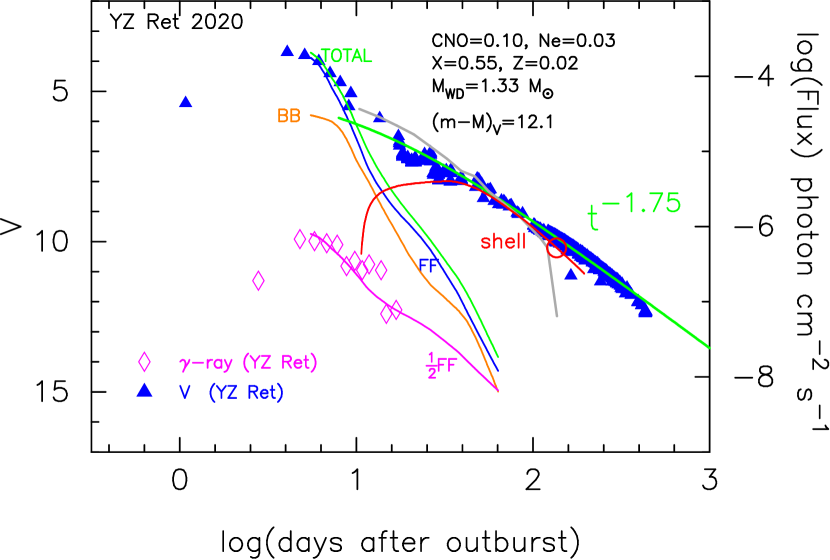
Figure 3: The optical $V$ (filled blue triangles) as well as the GeV gamma-ray (open magenta diamonds) light curves of YZ Ret 2020. The distance modulus in the $V$ band of $\mu_{V}\equiv(m-M)_{V}=12.1$ is assumed. A thick green line labeled $t^{-1.75}$ denotes the $t^{-1.75}$ decay trend in equation (2) with $(m-M)_{V}=12.1$ and $\Delta V=0.0$. We also plot our model light curves of the 1.33 $M_{\sun}$ WD (Ne2): photospheric blackbody (orange line labeled BB), free-free emission of optically thick winds (blue line labeled FF, calculated from equation (B3)), and the total of them (thin green line labeled TOTAL, calculated from equation (B4)). We further add the ${1\over 2}m_{\rm ff}$ model light curve (magenta line labeled ${1\over 2}$FF, calculated from equation (18)). The gray and red lines represent the time-stretched light curves of Kato et al. (2022a)’s fully self-consistent $1.0~{}M_{\sun}$ WD nova model with the stretching factor of $\log f_{\rm s}=-0.4$. The open red circle on the red line indicates the epoch when optically thick winds stop. The right edge of the red line corresponds to the epoch where the shock disappears. See Appendix B for more details of the model light curve calcualtions.

2.5 Supersoft X-ray source (SSS) phase

The X-ray flux (filled black squares) at the 0.3–2 keV band begins to rise drastically on $t_{0}+62$ day in Figure 1, indicating the appearance of the supersoft X-ray source (SSS) phase (Sokolovsky et al., 2020b). Then, it shows a flat peak between $t_{0}+63$ day and $\sim t_{0}+90$ day. After day $t_{0}+100$, the X-ray flux begins to decay.

Izzo et al. (2020) obtained the UVES spectra on $t_{0}+73$ day, which show broad (FWZI of H$\beta\sim 4000$ km s^-1) and strong forbidden lines emission of [O III] 4959/5007 Å, [O III] 4363 Å  blended with H$\gamma$, and [N II] 5755 Å. Balmer and He lines show a structured saddle-shaped profile suggesting non-spherical ejecta. Their preliminary analysis shows that the observed structure can be explained by a regular symmetric equatorial and polar outflow at an inclination of $\sim 60\arcdeg$. There appears to be a blue bump on all the unblended lines at $\sim-1250$ km s^-1, suggesting that the shell has not yet fully settled into its ’frozen’ nebular spectral line structure. They concluded that the nova erupted on an ONe white dwarf based on their spectra, which showed an overabundance of oxygen and the presence of strong [Ne III] 3342 Å  and [Ne V] 3426 Å  lines.

Sitko et al. (2020) reported their infrared spectroscopic observations on $t_{0}+91.8$ day and $t_{0}+124.8$ day. Their earlier observation showed that YZ Ret had entered the coronal stage, displaying strong infrared lines of [Si VI] and [Si VII], as well as [S VIII] and [Ca VIII], while the later observation showed new multiple lines of N V and significantly strengthened [Si VI] and [Si VII] lines. Most of the emission lines showed double peaked structure with large dips near line center, similar to what was reported for the optical lines in Izzo et al. (2020). Full widths at half maxima were slightly greater than 2000 km s^-1.

Figure 4: Shock properties for our 1.33 $M_{\sun}$ WD (Ne2) model (Hachisu & Kato, 2018b). Only the decay phase (after the optical maximum) of steady-state envelope model is plotted. Each abscissa is common, days after optical maximum, and the time $t=0$ correspond to the optical maximum. (a) Various photospheric properties: the wind mass-loss rate (black line, labeled ${\dot{M}}_{\rm wind}$), wind velocity (blue, $v_{\rm ph}$), photospheric radius (red, $R_{\rm ph}$), shock velocity (magenta, $v_{\rm shock}$). (b) Trajectories (straight black lines) of winds ejected at each time from the photosphere converge. A strong shock (solid red line) arises soon after the optical maximum and travels outward at a speed of $\sim$700–800 km s^-1. The blue line shows the position of the photosphere. (c) Temporal variation in the hydrogen column density $N_{\rm H}$ (blue line) behind the shock and the number density $n(R)$ (red line) just in front of the shock ($R=R_{\rm sh}$).

3 Light curve fitting of YZ Ret

In the present paper, we study the post-maximum phase using the steady-state wind mass-loss solutions because (1) fully self-consistent nova calculations are numerically time-consuming and difficult and (2) the decay phase of a nova is well described by a sequence of the steady-state wind solutions (Kato et al., 2022a).

We use steady-state wind models in Hachisu & Kato (2010), Hachisu & Kato (2016a), and Hachisu & Kato (2018b). These light curve models can be applied only to the decay phase of novae, but have been applied to the decay phases of a number of novae and have reasonably reproduced their light curves. The method of model light curve fittings are described in Hachisu & Kato (2015). We calculated the supersoft X-ray flux assuming blackbody photosphere for the energy range of 0.3–2 keV (Kato & Hachisu, 1994; Hachisu & Kato, 2010).

3.1 Model selection

Theoretical light curves of novae depend on the WD mass, chemical composition of the envelope, and mass-accretion rate. Kato et al. (2022b, c) estimated the WD mass to be between 1.3 and 1.35 $M_{\sun}$ for the mass accretion rate $\sim($2–5$)\times 10^{-9}$ $M_{\sun}$ yr^-1 (See Sections 2.2 and 2.3). Therefore, we examined 1.3, 1.33, and 1.35 $M_{\sun}$ WDs with the envelope chemical compositions of neon nova 2 (Ne2: $X=0.55$, $Y=0.30$, $Z=0.02$, $X_{\rm CNO}=0.10$, $X_{\rm Ne}=0.03$) and neon nova 3 (Ne3: $X=0.65$, $Y=0.27$, $Z=0.02$, $X_{\rm CNO}=0.03$, $X_{\rm Ne}=0.03$). Among them, the 1.33 $M_{\sun}$ WD (Ne2) model well reproduces the X-ray observation in the SSS phase (magenta lines in Figure 1). The X-ray flux of the 1.3 $M_{\sun}$ WD (Ne2) and 1.35 $M_{\sun}$ WD (Ne2) models sharply increases on $t_{0}+82$ day and $t_{0}+48$ day, and these two dates are too late and too early, respectively, to be consistent with the X-ray observation in Figure 1, in which we suppose that the X-ray turn-on time is $t_{0}+62$ day. Similarly, we exclude our 1.3 $M_{\sun}$ WD (Ne3), 1.33 $M_{\sun}$ WD (Ne3), and 1.35 $M_{\sun}$ WD (Ne3) models because their SSS-on day are $t_{0}+112$, $t_{0}+82$, and $t_{0}+65$ day, respectively.

3.2 Optical emission and shock formation

First, we calculated optical $V$ light curves in the early decay phase ($t<t_{0}+10$ day). In this phase, the observed $V$ light curve is well fitted with our model $V$ light curve (thin green line labeled TOTAL) as shown in Figures 1 and 3. Here, the total $V$ luminosity $L_{V,\rm total}$ is the summation of free-free emission $L_{V,\rm ff,wind}$ (blue line labeled FF) and photospheric emission $L_{V,\rm ph}$ (red or orange line labeled BB). The calculation method is introduced in Appendix B.

After $t_{0}+10$ day, our model light curve deviates largely from the $V$ observation. In this later phase, the shocked shell contributes to the $V$ luminosity.

Figure 4a depicts temporal variations of the photospheric radius $R_{\rm ph}$, velocity $v_{\rm ph}$, and wind mass-loss rate $\dot{M}_{\rm wind}$ as well as the shock velocity $v_{\rm shock}$ ($=$ the velocity of the shocked shell). Our steady-state wind model can be applied only to the post-maximum phase (Hachisu & Kato, 2006, 2015), so that we plot $R_{\rm ph}$, $v_{\rm ph}$, and $\dot{M}_{\rm wind}$ only in the decay phase of a nova, i.e., after the optical maximum.

In Figure 4b, we plot each locus of the wind particle, which is assumed to have a constant velocity after it was ejected from the photosphere. Each locus collides with each other and forms a shock (red line). We also depict the hydrogen column density $N_{\rm H}$ behind the shock front ($N_{\rm H}$ is the number density per unit area above the shock front) in Figure 4c. The initial increase in $N_{\rm H}$ near $t=0$ is an accumulation effect of the wind at the shock. We also add the number density of gas $n(R)$ just in front of the shock (at the radius $R$). Thus, we confirm that a strong shock arises soon after the optical peak and expands at about 800 km s^-1. Such an configuration of ejecta is illustrated in Figure 2c.

The photospheric velocity $v_{\rm ph}$ decreases with time before optical maximum and then turns to increase after that. Figure 4a shows $v_{\rm ph}$ of the decay phase of our 1.33 $M_{\sun}$ WD. In the decay phase, the later ejected matter catches up the earlier ejected gas after optical maximum (Figure 4b). Thus, the collision in the ejecta generates a shock after optical maximum. (See also Figure 8c in Appendix A, which clearly shows that the ejected wind velocity ($v_{\rm ph}$) in Kato et al. (2022a)’s model is decreasing before optical maximum but turns to increase after that.)

We estimate the flux of shell emission $L_{V,\rm shell}$ from the shocked shell configuration (equation (B6) in Appendix B). This is the contribution of free-free, bound-free, and bound-bound emissions. In Figure 3, we show this flux by the red line labeled “shell.” The shell flux increases at $t_{0}+10$ day and levels off until $t_{0}+40$ day, which is followed by a decline of $t^{-1.75}$, along with the thick green line labeled $-1.75$, in the nebular phase ($t\gtrsim t_{0}+40$ day). See Appendix B for more details of shell emission calculation.

3.3 Soft X-ray emission

YZ Ret entered the SSS phase on $t_{0}+62$ day as shown in Figure 1. In our $1.33~{}M_{\sun}$ WD (Ne2) model, the optically-thick winds stop on $t_{0}+62$ day and the nova enters the SSS phase. We illustrate this SSS phase in Figure 2d. The photosphere of the WD envelope shrinks to $R_{\rm ph}\lesssim 0.1~{}R_{\sun}$ on $\sim t_{0}+62$ day and the photospheric temperature becomes high (k$T_{\rm ph}\gtrsim 25$ eV) enough to emit soft X-rays. The X-ray flux (0.3–2.0 keV band) is calculated from blackbody assumption with $T_{\rm ph}$ and $L_{\rm ph}$. The model X-ray light curve begins to decrease on day $t_{0}+90$, being consistent with the observation.

Sokolovsky et al. (2022) obtained X-ray spectra on $t_{0}+78$ day with the XMM-Newton/RGS, which are dominated by emission lines. Such emission-line-dominated spectra strongly indicates a high inclination of the binary. The WD photosphere is occulted by the edge of an elevated accretion disk (e.g., Ness et al., 2013; Sokolovsky et al., 2022). It is consistent with the small X-ray fluxes during the SSS phase (see also Orio et al., 2022); the flux at the SSS phase is about ten times smaller than that at the X-ray flash phase on $t_{0}+0$ day (filled red square in Figure 1).

Izzo et al. (2020) observed YZ Ret with the UVES at ESO on $t_{0}+72$ day (JD 2,459,110.5) in the mid-SSS phase. In their high resolution spectra, Balmer and He lines show a structured saddle-shaped profile suggesting non-spherical ejecta. These observed structures can be explained by an equatorial and polar outflow at an inclination of $\sim 60\arcdeg$. Such a high inclination angle is also broadly consistent with the small soft X-ray flux and strong emission-line-dominated spectra of XMM-Newton/RGS.

Therefore, we plot two X-ray light curves (thin and thick magenta lines) in Figure 1. The thin magenta line shows the soft X-ray flux for no occultation, that is, for the case that the absorption is the same as that for the X-ray flash on $t_{0}+0$ day. We add the soft X-ray flux (thin magenta line) at the X-ray flash of the $1.3~{}M_{\sun}$ WD (on $t_{0}+0$ day), which is taken from Kato et al. (2022b). On the other hand, we plot the thick magenta line of our 1.33 $M_{\sun}$ WD (Ne2), the flux of which is set to follow a flat peak of the soft X-ray between $t_{0}+63$ and $\sim t_{0}+90$ day. This lower flux line corresponds to a twenty-seventh of the thin magenta line (for the case of no occulatation). The observational fluxes are broadly located between these two lines.

4 Emissions from a shocked shell

In this section, we examine how and why our $1.33~{}M_{\sun}$ WD model explains shock-associated observations such as optical spectra, hard X-rays, and GeV gamma-rays.

4.1 Multiple velocity systems in the ejecta

Nova ejecta show multiple velocity systems as described by McLaughlin (1942) and Mclaughlin (1943). Hachisu & Kato (2022) interpreted McLaughlin (1942)’s pre-maximum, principal, diffuse-enhanced absorption/emission line systems as those produced by the earliest wind before optical maximum, shocked shell, and inner wind, as illustrated in Figure 2b and 2c.

YZ Ret also shows multiple velocity systems. Sokolovsky et al. (2022) noticed two P Cygni velocity components of $-1200$ and $-2700$ km s^-1 (Aydi et al., 2020b, and private communication) on JD 2,459,046.67, i.e., $t_{0}+8.47$ day, about 4 days post-maximum. We regard these two velocities to be those of principal and diffuse enhanced, $v_{\rm p}=1200$ km s^-1 and $v_{\rm d}=2700$ km s^-1, respectively, instead of our shock model velocities of $v_{\rm shock}=800$ km s^-1 and $v_{\rm wind}=1200$ km s^-1, which tend to be smaller than the observation. Here, $v_{\rm p}$ is the velocity of the principal system and $v_{\rm d}$ that of the diffuse enhanced system.

Sokolovsky et al. (2022) estimated the ejecta mass in YZ Ret to be between $M_{\rm ej}=2\times 10^{-6}~{}M_{\sun}$ (for assumed $v_{\rm shell}=1200$ km s^-1 and $N_{\rm H}=7.3\times 10^{22}$ cm^-2) and $M_{\rm ej}=2\times 10^{-4}~{}M_{\sun}$ (for assumed $v_{\rm shell}=2700$ km s^-1 and $N_{\rm H}=131.3\times 10^{22}$ cm^-2), where $v_{\rm shell}=v_{\rm shock}=v_{\rm p}$ is the velocity of the shocked shell. Our $1.33~{}M_{\sun}$ WD model suggests $M_{\rm ej}=4\times 10^{-6}~{}M_{\sun}$. We also obtain $N_{\rm H}\sim 30\times 10^{22}$ cm^-2 (for $v_{\rm shell}=800$ km s^-1) from Figure 4c. Our estimates are broadly consistent with the above values.

4.2 Duration of shock

In our nova model, a shock arises just after the optical peak (see, e.g., Figures 2, 4, and Appendix Figure 8). The shock disappears when the wind stops. More accurately, the shock ends when the last wind reaches the shock front. The shock front is far outside the photosphere, so it takes $t_{\rm ret}$ days from the date of wind stopping at the photosphere to the time of shock termination. In the last day of the shock, the shock front is at $R_{\rm sh}(t)$. The winds collide with themselves forming the shock. The wind velocity is $v_{\rm wind}(t)=v_{\rm ph}(t-t_{\rm ret})$ at $R_{\rm sh}(t)$, because it was ejected from the photosphere $t_{\rm ret}$ days before the collision. This retarded (look back) time is $t_{\rm ret}=(R_{\rm sh}(t)-R_{\rm ph}(t-t_{\rm ret}))/v_{\rm ph}(t-t_{\rm ret})$, where $R_{\rm ph}(t-t_{\rm ret})$ and $v_{\rm ph}(t-t_{\rm ret})$ are the photospheric radius and velocity at $t-t_{\rm ret}$. Assuming that the last wind was emitted at the wind stopping time $t_{\rm ws}$, the shock duration of $\tau_{\rm shock}\equiv t_{\rm ws}+t_{\rm ret}$ is calculated from

$$(t_{\rm ws}+t_{\rm ret})v_{\rm sh}(t_{\rm ws}+t_{\rm ret})=t_{\rm ret}v_{\rm ph}(t_{\rm ws}),$$ (3)

where $v_{\rm sh}$ is the velocity of the shocked shell at $t_{\rm ws}+t_{\rm ret}$, $v_{\rm ph}$ the velocity at the photosphere at $t_{\rm ws}$. This simply means that the shock front moves with the speed of $v_{\rm sh}$ from the optical maximum and the last wind catches up the shock with the speed of $v_{\rm ph}$.

Our model predicts the shock duration by substituting $v_{\rm sh}\approx v_{\rm p}=1200$ km s^-1 (principal system), $v_{\rm ph}\approx v_{\rm d}=2700$ km s^-1 (diffuse enhanced system), and $t_{\rm ws}=58$ day (the wind duration just after the shock arises) into

$$\tau_{\rm shock}={{t_{\rm ws}}\over{\left(1-{{v_{\rm p}}\over{v_{\rm d}}}\right)}}.$$ (4)

The shock duration is $\tau_{\rm shock}=58/0.4444=104$ day. Therefore, we expect hard X-ray emission until about $t_{0}+110$ day in YZ Ret.

Izzo et al. (2020) pointed out that a blue bump appears at $\sim-1250$ km s^-1 on all the unblended lines in their $t_{0}+72$ day observation. Thus the shell has not yet fully settled into its ’frozen’ nebular structure. On the other hand, Galan & Mikolajewska (2020) reported that the nova shell has reached its ’frozen’ structure on $t_{0}+110$ day. Thus, the freezing occurred between $t_{0}+72$ day and $t_{0}+110$ day. This epoch is consistent with our result that the shock disappeared before $t_{0}+110$ day and then the shell entered the free expansion phase (no acceleration by shock).

McLoughlin et al. (2021) presented rapidly evolving spectroscopic sequences of YZ Ret, especially of the H$\alpha$ complex, from $t_{0}+8.76$ day to $t_{0}+175$ day. They found that the evolution trend of the H$\alpha$ velocity features changed on $t_{0}+100$ day. This epoch is broadly coincident with the end of shock in our model as mentioned above.

4.3 Rectangular line profiles: jets vs. shocked shell

Many novae showed a rectangular shape of emission lines in the nebular phase. Beals (1931) analyzed flat-top emission lines in the two classical novae, V476 Cyg 1920 and V603 Aql 1918, and concluded that such a rectangular profile arises from an optically-thin, spherical thin shell. The line width of a rectangle shape corresponds to $2v_{\rm shell}$.

In the present paper, we assume that the optically-thick winds and shocked shell are spherically symmetric as illustrated in Figure 2c and 2d. YZ Ret also showed a rectangular-like shape of emission lines of Balmer, O I, and Fe II (Aydi et al., 2020b; McLoughlin et al., 2021). This supports that an optically-thin, spherical shell is formed in the nova ejecta. Note that many photo-images of nova shells show almost spherically- or ellipsoidally-distributed blobs like in GK Per 1901 (e.g., Shara et al., 2012). Slavin et al. (1995) showed that the axis ratio of a nova shell is related to the nova speed class such that slower novae appear to have more elongated shells. Thus, spherically symmetric assumption is broadly consistent with observational features of the very fast nova class of YZ Ret ($t_{2}\approx 6$ day).

On the other hand, McLoughlin et al. (2021) proposed a ’jets’ model. They decomposed an emission line with a dip at the line center into two Gaussians; blue-shifted and red-shifted components, which correspond to near-coming and far-receding jets, respectively. If it is the case, many lines are originated from the jets. This simply means that a large part of the nova envelope is ejected in the jets. As a result, many novae should show a bi-polar geometry in the ejecta, which is against observations. See also, e.g., Hutchings (1972) for relations between line profiles with dips and non-spherical shells.

We have a possible reason why a line profile has a dip at the line center even for a spherical shell. If the geometrically-thin shell has small optical thickness (small but finite line optical depth $\tau$), the rectangular line profile becomes a “saw-toothed” shape with a dip at the line center (e.g., Wagenblast et al., 1983; Bertout & Magnan, 1987).

Sokolovsky et al. (2022) also argued against McLoughlin et al. (2021)’s jets model for YZ Ret. Their points are two-fold: (1) the line-dominated SSS phase in YZ Ret strongly suggests a high inclination angle of the binary. The observed velocities of $\sim 1000$ km s^-1 is too high to be compatible with the projected velocities of jets. (2) If blobs in the jet collide with each other and emits X-rays, its timescale is determined by the blob size, that should be short. This is against the observed long timescale. Therefore, the emitting region is relatively large.

4.4 Hard X-ray emission

The temperature just behind the shock is estimated to be

$$kT_{\rm sh} \sim {3\over 16}\mu m_{p}\left(v_{\rm wind}-v_{\rm shock}\right)^{2}$$ (5)

$$\approx 1.0{\rm~{}keV~{}}\left({{v_{\rm wind}-v_{\rm shock}}\over{1000{\rm~{}km~{}s}^{-1}}}\right)^{2},$$ (6)

where $k$ is the Boltzmann constant, $T_{\rm sh}$ is the temperature just after the shock (see, e.g., Metzger et al., 2014), $\mu$ is the mean molecular weight ($\mu=0.5$ for hydrogen plasma), and $m_{p}$ is the proton mass. Substituting $v_{\rm shock}=v_{\rm p}=1200$ km s^-1 and $v_{\rm wind}=v_{\rm d}=2700$ km s^-1, we obtain the post-shock temperature $kT_{\rm sh}\sim 2.3$ keV.

Mechanical energy of the wind is converted to thermal energy by the reverse shock (Metzger et al., 2014) as

$$L_{\rm sh} \sim {{9}\over{32}}{\dot{M}}_{\rm wind}{{(v_{\rm wind}-v_{\rm shock})^{3}}\over{v_{\rm wind}}}$$ (7)

$$= 1.8\times 10^{37}{\rm~{}erg~{}s}^{-1}\left({{{\dot{M}}_{\rm wind}}\over{10^{-4}~{}M_{\sun}{\rm~{}yr}^{-1}}}\right)$$ (9)

$$\times\left({{{v_{\rm wind}-v_{\rm shock}}\over{1000{\rm~{}km~{}s}^{-1}}}}\right)^{3}\left({{{1000{\rm~{}km~{}s}^{-1}}\over{v_{\rm wind}}}}\right).$$

Substituting $\dot{M}_{\rm wind}=0.5\times 10^{-4}~{}M_{\sun}$ yr^-1 from Figure 4a, we obtain the post-shock energy of $L_{\rm sh}\sim 1.1\times 10^{37}$ erg s^-1.

Sokolovsky et al. (2022) analyzed the NuSTAR observation of YZ Ret on $t_{0}+10.7$ day. They fitted a single temperature thermal plasma model with the observed spectrum (3.5–78.5 keV) and obtained $kT=6.5\pm 1.5$ keV and $N_{\rm H}=20^{23}$–$10^{24}$ cm^-2, depending on abundances. Our $1.33~{}M_{\sun}$ WD (Ne2) model gives $kT_{\rm sh}=2.3$ keV and $N_{\rm H}\sim 2\times 10^{23}$ cm^-2 on the same day, which are broadly consistent with the results by Sokolovsky et al. (2022).

In the later nebular and SSS phases, the velocity and mass of shocked shell do not change so much. The column density of hydrogen is estimated from $M_{\rm shell}=4\pi R_{\rm sh}^{2}\rho h_{\rm shell}$, where $\rho$ is the density in the shocked shell, and $h_{\rm shell}$ the thickness of the shocked shell. If we take an averaged velocity of shell $v_{\rm sh}=v_{\rm shell}=v_{\rm shock}$, the shock radius is calculated from $R_{\rm sh}(t)=v_{\rm shock}\times t$. This reads

$$N_{\rm H} = {{X\over m_{p}}{{M_{\rm shell}}\over{4\pi R^{2}_{\rm sh}}}}$$ (10)

$$\approx 4.8\times 10^{22}{\rm~{}cm}^{-2}\left({X\over{0.5}}\right)\left({{M_{\rm shell}}\over{10^{-5}M_{\sun}}}\right)\left({{R_{\rm sh}}\over{10^{14}{\rm~{}cm}}}\right)^{-2}$$ (11)

$$\approx 6.4\times 10^{20}{\rm~{}cm}^{-2}\left({X\over{0.5}}\right)\left({{M_{\rm shell}}\over{10^{-5}M_{\sun}}}\right)$$ (13)

$$\times\left({{v_{\rm shell}}\over{1000{\rm~{}km~{}s}^{-1}}}\right)^{-2}\left({{t}\over{100~{}{\rm day}}}\right)^{-2}.$$

This gives $N_{\rm H}\approx 3\times 10^{20}$ cm^-2 for $M_{\rm shell}=0.5\times 10^{-5}~{}M_{\sun}$, $v_{\rm shell}=1200$ km s^-1, and $t=90$ day, which is the end of the supersoft X-ray source phase.

Pei et al. (2020) and Orio et al. (2022) analyzed the NICER observation (0.3–2 keV) of YZ Ret on $t_{0}+83$ and $t_{0}+84$ day and obtained $T_{\rm ph}=$500,000–550,000 K and $N_{\rm H}=3\times 10^{20}$ cm^-2, which is consistent with our estimate mentioned above.

4.5 GeV gamma-ray emission

Recently gamma-rays were often detected during nova outbursts (e.g., Ackermann et al., 2014). GeV gamma-rays were also observed in the YZ Ret outburst with the Fermi/Large Area Telescope (LAT) (Sokolovsky et al., 2022). Such gamma-rays are considered to originate from strong shocks (see, e.g., Chomiuk et al., 2021, for a recent review). The gamma-ray flux peaked on JD 2,459,042.99 ($t_{0}+4.79$ day) (König et al., 2022), slightly later than the brightest $V$ observation ($V=3.7$ at $t_{0}+4.06$ day), as already introduced in Section 2.3. This epoch of appearance is consistent with our shock model.

The gamma-ray fluxes (open magenta diamonds) in Figure 3 broadly follows the trend of optical $V$ decay. In our model, the optical flux is dominated by free-free emission and is given by $L_{V,\rm ff}\propto(\dot{M}_{\rm wind}/v_{\rm ph})^{2}\propto f(t)$ (equation (B2)) while the gamma-ray flux is given by $L_{\gamma,\rm sh}\propto(\dot{M}_{\rm wind}/v_{\rm wind})\propto[f(t)]^{1/2}$ (equation (9)), where $f(t)$ is a function of time $t$. Thus, the dependencies of $L_{V,\rm ff}$ and $L_{\gamma,\rm sh}$ on $(\dot{M}/v)^{n}$ is similar, but the power of $n$ is different by a factor of two ($n=2$ vs $n=1$). Therefore, the light curves in magnitudes are written as

$$m_{\gamma,\rm sh}(t) = -2.5\log L_{\gamma,\rm sh}+{\rm~{}const.}$$ (14)

$$= -2.5\log[f(t)]^{1/2}+{\rm~{}const.}$$ (15)

$$= {1\over 2}\left(-2.5\log f(t)+{\rm~{}const.}\right)$$ (16)

$$= {1\over 2}(-2.5\log L_{V,\rm ff}+{\rm~{}const.})$$ (17)

$$= {1\over 2}m_{V,\rm ff}(t)+{\rm~{}const}.,$$ (18)

so the decay slope is slow by a factor of 2. Here, the proportionality constant is included in the term “const.” We plot the $m_{\gamma,\rm sh}$ (cyan line labeled ${1\over 2}$FF) in Figures 1 and 3. This model slope represents well the decay trend of GeV gamma-ray fluxes.

Sokolovsky et al. (2022) obtained the flux of GeV gamma-ray (0.1–300 GeV) to be $L_{\gamma}=3\times 10^{35}$ erg s^-1 and the optical luminosity to be $L_{\rm opt}=7\times 10^{38}$ erg s^-1 on $t_{0}+4.1$ day. The gamma to optical ratio is $L_{\gamma}/L_{\rm opt}=4\times 10^{-4}$. In our model, the shock energy generation is $L_{\rm sh}=1.1\times 10^{37}$ erg s^-1. The ratio of $L_{\gamma}/L_{\rm sh}=0.027$, about 3% conversion rate, is consistent with

$$L_{\gamma}=\epsilon_{\rm nth}\epsilon_{\gamma}L_{\rm sh}\lesssim 0.03~{}L_{\rm sh},$$ (19)

where $\epsilon_{\rm nth}\lesssim 0.1$ is the fraction of the shocked thermal energy to accelerate nonthermal particles and $\epsilon_{\gamma}\lesssim 0.1$ the fraction of this energy radiated in the Fermi/LAT band (typically $\epsilon_{\rm nth}\epsilon_{\gamma}<0.03$, Metzger et al., 2015).

Figure 5: The $V$ (and $y$) light curves of V1668 Cyg (a) and V1974 Cyg (b). The $V$ and $y$ data are the same as those in Hachisu & Kato (2016b). The blue lines denote the total $V$ luminosity of our models. The open blue circle at the right edge of each blue line corresponds to the epoch when optically thick winds stop. The gray and red lines indicate the $V$ luminosities of wind and shell emission, respectively, of Kato et al. (2022a)’s fully self-consistent nova model, as summarized in Appendicies A and B. The open red circle on the red line indicates the epoch when optically thick winds stop. The right edge of the red line corresponds to the epoch when the shock disappears. (a) V1668 Cyg. We adopt the time-stretching factor of $\log f_{\rm s}=-0.34$ for the fully self-consistent nova model (gray and red lines). The green line labeled $t^{-1.75}$ shows equation (2) with $(m-M)_{V}=14.6$ and $\Delta V=-0.2$ (b) V1974 Cyg. We adopt $\log f_{\rm s}=-0.38$. The green line labeled $t^{-1.75}$ denotes equation (2) with $(m-M)_{V}=12.0$ and $\Delta V=-0.2$.

5 Extension of the universal decline law to the nebular phase

Hachisu & Kato (2006) theoretically proposed a $t^{-1.75}$ decay of free-free emission luminosity. This decline law explains many classical novae light curves. Therefore, it has been named the universal decline law. However, Hachisu & Kato (2006)’s model light curve of $L_{V,\rm ff}$ (blue line) begins to deviate from the $V$ observation after the nova entered the nebular phase, as in Figures 5, 6, 7, and Appendix Figure 10. This clearly suggests that emissions from the shocked shell contribute significantly to the $V$ flux of the nova after the nebular phase starts. We suppose that equation (2) represents a temporal variation of the $V$ flux from such a shell emission.

It should be noted here that the universal decline law indicates $L_{V,\rm ff}\propto(t-t_{0})^{-1.75}$. This curve is slightly different from that of equation (2), because we derived equation (2) from the direct fit with the YZ Ret $V$ light curve for $t\gtrsim t_{0}+10$ day. Large differences from the $(t-t_{0})^{-1.75}$ universal decline law come from the term $(t-t_{0}+10{\rm~{}day})^{-1.75}$ in equation (2). However, the difference between the two laws becomes small for $t-t_{0}\gg 10{\rm~{}day}$.

In this section, we explain how this trend of $L_{V}\propto t^{-1.75}$ can be applied to the nebular phase of the other novae. The flux of shell emission is calculated based on Kato et al. (2022a)’s fully self-consistent nova model. We apply this shell luminosity to each nova with the time-stretching method (Hachisu & Kato, 2018b): two nova light curves of different speed class overlap each other, if the timescale of one of them is squeezed by a factor of $f_{\rm s}$, i.e., as $t/f_{\rm s}$, and its absolute $V$ brightnesses is shifted to be $M_{V}-2.5\log f_{\rm s}$. In other words, the two nova light curves overlap each other in the $(t/f_{\rm s})$-$(M_{V}-2.5\log f_{\rm s})$ plane. (See appendix B for more detail.) We pick up seven well observed novae among what we have already studied. LV Vul is examined as an example in appendix B. We show the other six novae as follows: The red line in each figure denotes the shell luminosity, whereas the blue line indicates our model flux of $L_{V,\rm total}=L_{V,\rm ff}+L_{V,\rm ph}$ calculated from optically thick winds. The red line is for Kato et al. (2022a)’s 1.0 $M_{\sun}$ WD model, but we overlap it with each nova light curve with the time-stretching method.

5.1 V1668 Cyg 1978

Figure 5a shows the wide $V$ band magnitudes (filled blue triangles) and intermediate $y$ band magnitudes (filled magenta circles) of V1668 Cyg. We adopt a $0.98~{}M_{\sun}$ WD (CO3) model light curve (Hachisu & Kato, 2016a). In the figure, our model light curve (blue line) well follows the $V$ and $y$ light curves from day $\sim 4$ to day $\sim 100$, while the $V$ and $y$ light curves depart from each other on day $\sim 100$.

The model light curve (blue line) follows the $y$ light curve rather than the $V$ light curve. While the wide $V$ band includes strong emission lines such as [O III], the free-free emission model light curve does not include them (strong emission lines). On the other hand, the intermediate $y$ band is designed to avoid strong emission lines such as [O III] (see, e.g., Figure 1 of Munari et al., 2013) and follows continuum flux (Lockwood & Millis, 1976).

The $V$ light curve itself seems to split slightly on day $\sim 55$. This difference comes from the sensitivity of each filter system. In the nebular phase, the strong nebular [O III] 4958.9 and 5006.9 Å  emission lines are located just at the blue edge of the $V$ bandpass (see, e.g., Figure 1 of Munari et al., 2013) and a small difference in the sensitivities of the two filters make a substantial difference in their $V$ magnitudes. This kind of split in the $V$ magnitude at the different observatories can be seen on day $\sim 65$ in V1974 Cyg (see Figure 5b). Thus, the splitting in $V$ magnitude indicates the beginning of the nebular phase.

In Figure 5a, our model light curve (blue line) crosses the red line on day $\sim 55$. After that, the shell emission dominates the total $V$ flux of the nova. We overplot the $t^{-1.75}$ decline law (green line) of equation (2) with $(m-M)_{V}=14.6$ and $\Delta V=-0.2$. This line represents well the $V$ light curve in the nebular phase of V1668 Cyg (after day $\sim 55$).

5.2 V1974 Cyg 1992

Figure 5b show the $V$ band magnitudes (filled blue circles) of V1974 Cyg. We adopt a $0.98~{}M_{\sun}$ WD (CO3) model light curve (Hachisu & Kato, 2016a). In the figures, our model light curve (blue line) well follows the $V$ light curves from day $\sim 6$ to day $\sim 100$. The $V$ light curve splits into two branches on day $\sim 65$, where the nebular phase started (e.g., Hachisu & Kato, 2016b).

In Figure 5b, The blue line crosses the red line on day $\sim 65$, suggesting that the shell luminosity dominates the $V$ flux of the nova. This is almost the same day that the nebular phase started.

We also overplot the $t^{-1.75}$ decline law (green line) of equation (2) with $(m-M)_{V}=12.0$ and $\Delta V=-0.2$. This green line follows both the red line and the lower branch of the $V$ light curve in the nebular phase of V1974 Cyg (after day $\sim 65$).

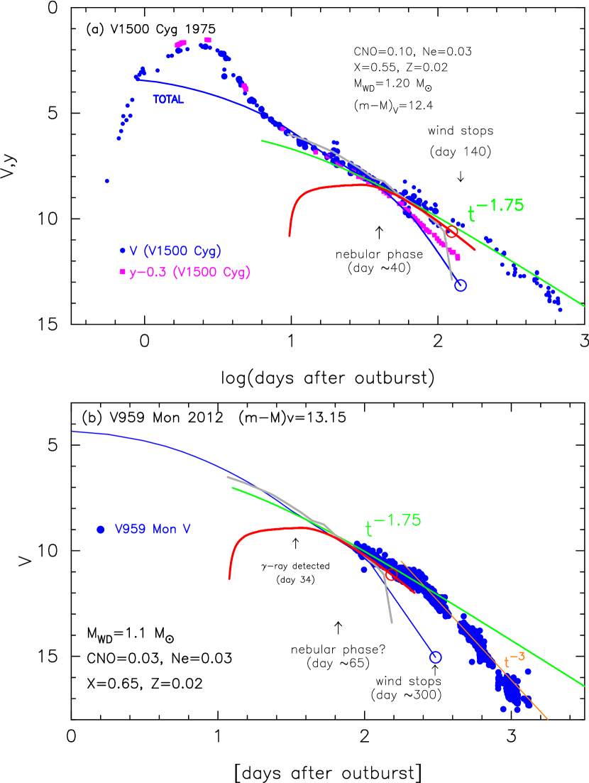
Figure 6: Same as Figure 5, but for V1500 Cyg and V959 Mon. (a) V1500 Cyg. The $V$ and $y$ data are the same as those in Hachisu & Kato (2016b). We adopt the time-stretching factor of $\log f_{\rm s}=-0.44$ for the fully self-consistent nova model (gray and red lines). The green line shows equation (2) with $(m-M)_{V}=12.4$ and $\Delta V=+0.3$. (b) V959 Mon. The $V$ data are taken from Hachisu & Kato (2018a). The time-stretching factor is $\log f_{\rm s}=-0.35$. The green line shows equation (2) with $(m-M)_{V}=13.15$ and $\Delta V=-0.35$. The decline law of $\propto t^{-3}$ (orange line) denotes emission from a freely-expanding shell after the shock disappeared.

5.3 V1500 Cyg 1975

Figure 6a shows the wide $V$ band magnitudes (filled blue circles) and intermediate $y$ band magnitudes (open magenta circles) of V1500 Cyg. The early 1–4 day broadband spectra can be fitted well with a black body (e.g., Gallagher & Ney, 1976). Then, the optical and IR spectra changed from blackbody to free-free emission on day 4–5 (after the outburst) as discussed by Gallagher & Ney (1976) and Ennis et al. (1977). In the figures, our model light curve (blue line) well follows the $V$ and $y$ light curves from day $\sim 5$ to day $\sim 40$.

We adopt a $1.2~{}M_{\sun}$ WD (Ne2) model (Hachisu & Kato, 2014). The $V$ and $y$ light curves depart from each other on day $\sim 40$, where the nebular phase starts (e.g., Hachisu & Kato, 2016b).

Hachisu & Kato (2016a) obtained the start of the nebular phase to be $V=8.5$, where the $y$ light curve (open magenta circles) separates from the $V$ light curve (filled blue circles). Our model light curve (blue line) follows the $y$ light curve rather than the $V$ light curve as shown in Figure 6a.

As for the other sources, we add the shell emission light curve which exceeds the blue line on day $\sim 40$. This is almost the same day that the nebular phase started. Therefore, in the nebular phase, the shell emission dominates the $V$ flux of the nova. We also add the $t^{-1.75}$ decline law (green line) of equation (2) with $(m-M)_{V}=12.4$ and $\Delta V=+0.3$. This green line follows both the red line and the $V$ light curve in the nebular phase of V1500 Cyg (after day $\sim 60$).

5.4 V959 Mon 2012

Figure 6b shows the $V$ band magnitudes (filled blue circles) of V959 Mon. This nova was detected in GeV gamma-rays with the Fermi/LAT (Ackermann et al., 2014) before the optical discovery by S. Fujikawa on UT 2012 August 9.8 (JD 2,456,149.3) at mag 9.4 (Fujikawa et al., 2012). Due to solar conjunction, the nova already entered the nebular decline phase when it was discovered. The optical peak was possibly substantially (more than 50 days) before the discovery (e.g., Munari et al., 2013).

We adopt a $1.1~{}M_{\sun}$ WD (Ne3) model light curve (Hachisu & Kato, 2018a). In the figure, our day 0 (outburst day) is set to be JD 2,456,066.5 after Hachisu & Kato (2018a), 34 days before the first gamma-ray detection at JD 2,456,100.5 (= UT 2012 June 22). The model light curve begins to deviate from the $V$ light curves from day $\sim 100$, where the nebular phase had already started (Munari et al., 2013). Comparing the $y$ and $V$ magnitude developments, Munari et al. (2013) concluded that a bifurcation between $y$ and $V$ light curves took place at the start of supersoft X-ray source phase, $\sim 200$ days after the outburst. After that, strong emission lines such as [O III] 4958.9 and 5006.9 Å  begins to contribute to the $V$ band magnitudes (see, e.g., Figure 1 of Munari et al., 2013).

As for the other emission, the shell emission line crosses the blue line on day $\sim 65$, suggesting that the shell emission luminosity dominates the $V$ flux of the nova. The nebular phase possibly started near above day $\sim 65$. We also overplot the $t^{-1.75}$ decline law (green line) of equation (2) with $(m-M)_{V}=13.15$ and $\Delta V=-0.35$. This green line follow the $V$ light curve in the nebular phase until day $\sim 260$.

After that, the $V$ light curve declines along $L_{V}\propto t^{-3}$ line (orange line labeled $t^{-3}$), where $L_{V}$ is the $V$ band flux. This rapid decline can be understood from a new condition that the thickness of the shell increases with time in equation (B6), i.e., $h=h_{0}\times(t/260~{}{\rm day})$ for $t>260$ day. On day $\sim 300$, optically-thick winds stop and we expect that the shock and the resultant compression at the shocked shell becomes weak, which is not able to keep the thickness $h$ nearly constant.

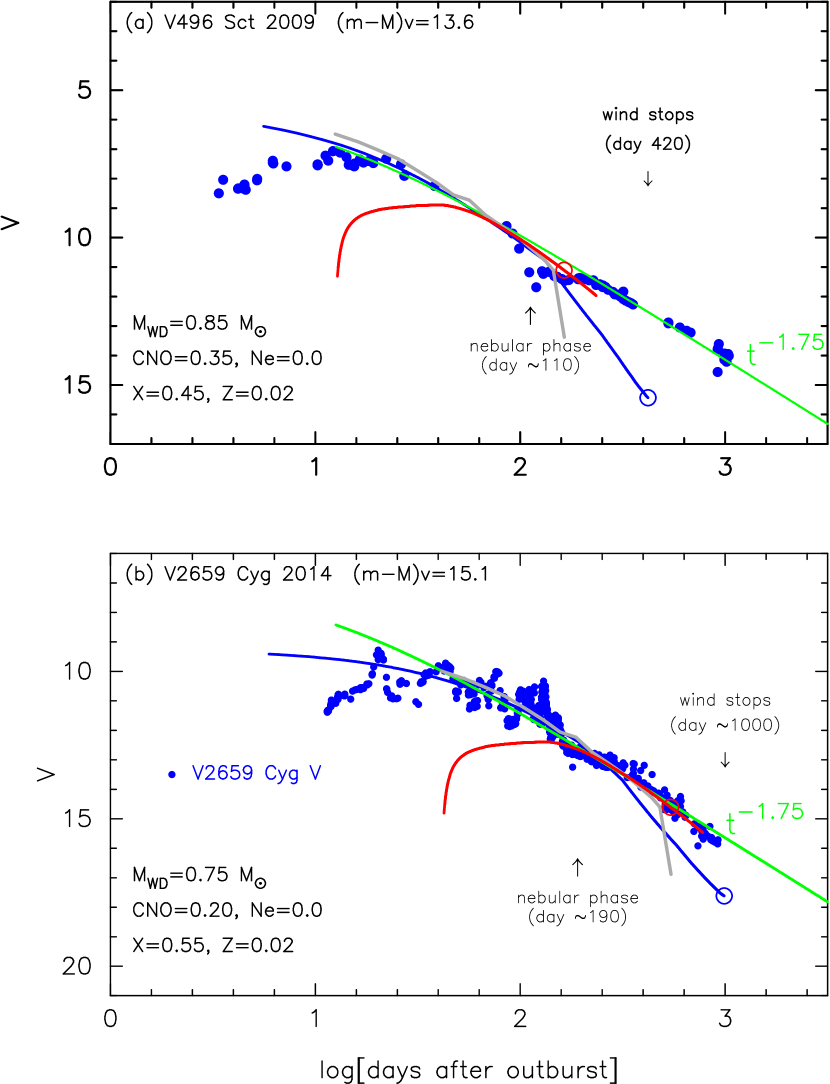
Figure 7: Same as Figure 5, but for V496 Sct and V2659 Cyg. The $V$ data of V496 Sct are taken from AAVSO and Raj et al. (2012), while those of V2659 Cyg are the same as those in Hachisu & Kato (2021). (a) V496 Sct. We adopt the time-stretching factor of $\log f_{\rm s}=-0.32$. The green line shows equation (2) with $(m-M)_{V}=13.6$ and $\Delta V=-0.9$. (b) V2659 Cyg. The time-stretching factor is $\log f_{\rm s}=+0.2$. The green line represents equation (2) with $(m-M)_{V}=15.1$ and $\Delta V=-0.9$.

5.5 V496 Sct 2009

Figure 7a shows the $V$ band magnitudes (filled blue circles) of V496 Sct. The $V$ data are taken from Raj et al. (2012) and the archive of the American Association of Variable Star Observers (AAVSO). We adopt a $0.85~{}M_{\sun}$ WD (CO3) model and the distance modulus in the $V$ band of $(m-M)_{V}=13.6$ from Hachisu & Kato (2021). Our model light curve (blue line) broadly follows the $V$ light curve from day $\sim 20$ to day $\sim 100$, although the $V$ observation has a small dip around day $\sim 110$. Dust grows in the shocked shell and absorbs optical fluxes both from free-free emission and shell emission. This absorption by a dust shell is the so-called “dust blackout.” Here, we set the outburst day (day 0) as JD 2,455,142.0 (= UT 2009 November 6.5), 12.2 days before the optical maximum at $V=7.07$ (Raj et al., 2012).

Raj et al. (2012) obtained a spectrum in the nebular phase 114 days after optical maximum, that is, day 126 in our Figure 7a. This date is close to the epoch of a shallow dust blackout. Thus, the nebular phase started around day $\sim 110$. Our total flux of BB+FF (blue line) also depart from the $V$ (filled blue circles) light curve around the same epoch.

The blue line crosses the red line on day $\sim 110$, suggesting that the shell luminosity dominates the $V$ flux of the nova. We also overplot the $t^{-1.75}$ decline law (green line) of equation (2) with $(m-M)_{V}=13.6$ and $\Delta V=-0.9$. The green line follows the red line at least from day $\sim 80$ to day $\sim 160$, and the $V$ light curve from day $\sim 200$ to day $\sim 1000$.

5.6 V2659 Cyg 2014

Figure 7b shows the $V$ band magnitudes (filled blue circles) of V2659 Cyg. We adopt a $0.75~{}M_{\sun}$ WD (CO4) (Hachisu & Kato, 2021). The model light curve (blue line) reasonably follows the $V$ light curve from day $\sim 15$ to day $\sim 300$, although the $V$ light curve is not smoothly declining but sometimes shows spikes and flares. Here, we set the outburst day as JD 2,456,737.0, 18.5 days before the $V$ maximum at $V=9.4$ mag (e.g., Tarasova, 2016). Tarasova (2016) mentioned, based on her optical spectra 146 days after the $V$ maximum, that the nova was in an early phase of the nebular stage. Her next spectra were obtained on 166 and 192 days after the $V$ maximum, which clearly show nebular emission lines such as [O III]. Therefore, the nova entered the nebular phase $\sim 160-170$ days after the optical maximum.

The blue line crosses the red line on day $\sim 190$, suggesting that the shell luminosity dominates the $V$ flux of the nova. The nebular phase possibly started near day $\sim 190$, which is consistent with the start day proposed by Tarasova (2016), i.e., $170+18.5\approx 190$ days after the outburst. We also overplot the $t^{-1.75}$ decline law (green line) of equation (2) with $(m-M)_{V}=15.1$ and $\Delta V=-0.9$. This green line follows the $V$ light curve in the nebular phase of V2659 Cyg.

6 Conclusions

We proposed a multiwavelength light curve model for the classical nova YZ Ret 2020, especially for the decay phase. Our main results are summarized as follows:

1. Our model $V$ light curve of free-free emission for a $1.33~{}M_{\sun}$ WD (Ne2) well reproduces the early decay phase until $t_{0}+10$ day.

2. After $t_{0}+10$ day, we modeled a $V$ light curve supposing that the optical emission mainly comes from the shocked shell. We found that the flux follows approximately the decay trend of $\propto t^{-1.75}$. This is the same trend as the universal decline law proposed by Hachisu & Kato (2006) for free-free emission. Thus, the decline trend of $L_{V}\propto t^{-1.75}$ can be applied from the early decline phase (dominated by free-free emission of winds) through the nebular phase (dominated by shocked shell emission) until the shock disappears.

3. The same 1.33 $M_{\sun}$ WD model reproduces the X-ray light curve of YZ Ret, from $t_{0}+62$ day to $\sim t_{0}+100$ day, i.e., the supersoft X-ray source (SSS) phase. The peak flux of the SSS phase is about a tenth of the flux at the X-ray flash. Because we directly observed the WD photosphere at the X-ray flash, the low flux during the SSS phase can be explained by an occultation of the WD surface.

4. A nova ejecta is divided by the shock into three parts, outermost expanding gas (earliest wind before maximum), shocked shell, and inner fast wind. These three are responsible for the pre-maximum, principal, and diffuse enhanced absorption/emission line systems, respectively. We interpret that the shock velocity $v_{\rm shock}$ corresponds to the velocity $v_{\rm p}$ of the principal system and the inner wind velocity $v_{\rm wind}$ to the velocity $v_{\rm d}$ of the diffuse enhanced system. The shock temperature is calculated to be $kT_{\rm sh}\sim 2.3$ keV from equation (6), assuming $v_{\rm p}=1200$ km s^-1 and $v_{\rm d}=2700$ km s^-1. This temperature and the hydrogen column density behind the shock on $t_{0}+10.7$ day are roughly consistent with the estimates by Sokolovsky et al. (2022).

5. Our shocked energy post-maximum is $L_{\rm sh}\sim 1.1\times 10^{37}$ erg s^-1, calculated from equation (9). The observed GeV gamma-ray energy is $L_{\gamma}\sim 3\times 10^{35}$ erg s^-1 (Sokolovsky et al., 2022). The ratio of $L_{\gamma}/L_{\rm sh}\sim 0.027$ satisfies the theoretical request ($L_{\gamma}/L_{\rm sh}\lesssim 0.03$, Metzger et al., 2015).

6. The shocked energy generation rate depends roughly on $\propto{\dot{M}}_{\rm wind}/v_{\rm wind}$ and the free-free emission flux depends differently on $\propto{(\dot{M}}_{\rm wind}/v_{\rm wind})^{2}$. Therefore, the decay trend of gamma-ray is roughly half as fast as that of optical, i.e., $m_{\gamma,\rm sh}={1\over 2}m_{V,\rm ff}+$const. in magnitude. This relation broadly reproduces the decay of GeV gamma-ray flux observed with Fermi/LAT.

7. We estimate the duration of the shock alive based on our shock model from equation (4), that is, the shock continues from $t_{0}+3$ day to $t_{0}+110$ day. The end of the shock indicates that the shocked shell begins to expand freely without significant acceleration. The event causes the freezing of emission line features. This epoch of $t_{0}+110$ day is consistent with the spectroscopic observations by Izzo et al. (2020), Galan & Mikolajewska (2020), and McLoughlin et al. (2021).

8. The above shocked-shell-emission model can be applied to the nebular phase of other novae. We show that the decline trend of $L_{V}\propto t^{-1.75}$ is common in the nebular phases of V1668 Cyg, V1974 Cyg, V1500 Cyg, V959 Mon, V496 Sct, V2659 Cyg, and LV Vul.

Appendix A One cycle of a nova outburst

In the present paper we adopt the 1.33 $M_{\sun}$ WD (Ne2) model for YZ Ret. This model is based on the steady-state approximation, that can be applied only to the decay phase (i.e., after optical maximum) of a nova outburst. The decay phase is only a part of one cycle of a nova outburst. This appendix gives a supplemental information for a nova outburst evolution.

A.1 HR diagram

Figure 8a shows the HR diagram for one cycle of a nova outburst (Kato et al., 2022a). This model is calculated with the fully consistent evolution method, in which the internal structure, from the white dwarf (WD) center to the photosphere, is consistently connected with the outer wind solution. Winds are accelerated by radiation pressure gradients, deep inside the photosphere, the so-called optically thick winds. This model is for a $1.0~{}M_{\sun}$ WD with the mass accretion rate to the WD before the outburst of ${\dot{M}}_{\rm acc}=5\times 10^{-9}$ $M_{\sun}$ yr^-1, different from our YZ Ret model, but this is only the fully self-consistent model of a classical nova outburst. The WD mass and mass-accretion rate are typical for classical novae, so we take this model as a representative of a nova outburst in the following explanation.

In the present work, we analyzed the YZ Ret observation for four different stages as in Figure 2. These stages correspond to four colored regions in the HR diagram (Figure 8a), that is, the X-ray flash (red), rising phase (cyan blue), decay phase (blue), and SSS phase (orange).

Timescale of each phase and physical values depend on the WD mass and mass-accretion rate. In the $1.0~{}M_{\sun}$ WD model, the temperature at point C is $3.8\times 10^{5}$ K, which is insufficient to emit strong X-ray flux. Kato et al. (2022a) calculated the X-ray and UV light curves and showed most of the energy is emitted in the UV band, and the X-ray flux is very weak. Thus, no X-ray flash is expected in less massive WDs than $1.0~{}M_{\sun}$. In more massive WDs ($>1.3~{}M_{\sun}$), on the other hand, their one cycle loops are located on the upper-left side of the $1.0~{}M_{\sun}$ WD. The temperature $T_{\rm ph}$ at point C increases up to 600,000–1,000,000 K and a very bright X-ray flash is expected. The duration of the flash is very short in massive WDs (Kato et al., 2022b, c).

The maximum temperature in the X-ray flash (point C) is lower than that in the SSS phase (Figure 8a). This property is common for all the WD masses and mass accretion rates. Thus, the peak luminosity of the X-ray flash should be lower than that in the SSS phase. Nevertheless, in YZ Ret, the observed X-ray flux in the SSS phase is about ten times smaller than in the X-ray flash detected with the SRG/eROSITA (König et al., 2022), as in Figure 1. Thus, the reason for this lower flux could be an occultation of the WD photosphere/surface by an elevated disk. This is consistent with the emission-line-dominated spectra in the SSS phase (Sokolovsky et al., 2022).

A.2 Optically Thick Winds

There is no indication of wind mass-loss in the X-ray flash phase of YZ Ret (König et al., 2022) and the spectrum is well represented by a blackbody spectrum of $T=3.3\times 10^{5}$ K. This is consistent with the theoretical calculation for a 1.0 $M_{\sun}$ WD (Kato et al., 2022a) in which optically thick winds are not accelerated in the very early phase but begin to blow when the photospheric temperature decreases to point E in Figure 8a.

In the very early phase of shell flash (from point B to C), convection widely occurs in the envelope that carries nuclear energy efficiently to the surface and the envelope does not expand. The envelope begins to expand when the envelope becomes radiative from the surface region. In the radiative region, opacity is an important factor for wind acceleration. The radiative opacity has a large peak corresponding to the iron ionization at $T\sim 2\times 10^{5}$ K (Iglesias & Rogers, 1996). In the case of our $1.0~{}M_{\sun}$ WD, optically thick winds start to blow at point E ($\log T$ (K)= 5.319). As the envelope expands and the photospheric temperature decreases, the density in the wind acceleration region increases with time. Thus, the wind mass loss rate increases, too.

Stage G in Figure 8a is the maximum expansion of the photosphere. The photospheric temperature reaches minimum. The wind mass-loss rate reaches maximum. The wind velocity at the photosphere decreases and reaches minimum at the same epoch. Their temporal variations are plotted in Figure 8b.

The velocities in Figure 8b are smaller than typical absorption line velocities of fast novae (1000–2000 km s^-1) but consistent with those of slow and very slow novae (200–800 km s^-1) as in Figure 11 of Aydi et al. (2020a). The velocity of wind $v_{\rm ph}$ at the photosphere decreases toward the maximum expansion of the photosphere and then increases. This trend in the photospheric velocity $v_{\rm ph}$ is commonly observed in many novae (e.g., Aydi et al., 2020a).

A.3 Formation of a strong shock outside the photosphere

Strong shocks have been suggested from recent detection of gamma-rays and hard X-rays in nova outbursts (e.g., Ackermann et al., 2014). Such high energy photons are assumed to originate from internal shocks in nova ejecta (e.g., Metzger et al., 2014, 2015; Martin et al., 2018; Chomiuk et al., 2021). However, no theoretical calculations of thermonuclear runaway show a shock wave formation, i.e., no shock arises inside the envelope including the nuclear burning region up to the photosphere. It is mainly because the timescale of nuclear energy generation ($\sim 100$ s) is much longer than the hydrodynamic timescale ($\sim 0.4$ s) in the hydrogen-burning zone (see Kato et al., 2022a; Hachisu & Kato, 2022, for more detail).

Figure 8: A fully self-consistent nova model on a $1.0~{}M_{\sun}$ WD with a mass accretion rate of $5\times 10^{-9}~{}M_{\sun}$ yr^-1, which is taken from Kato et al. (2022a). A shock model corresponding to this nova model is taken from Hachisu & Kato (2022). (a) The HR diagram. A: Quiescent phase before a shell flash. B: The epoch when the nuclear luminosity reaches maximum ($t=0$). C: The photospheric temperature takes the maximum value in the rising phase. E: The wind mass loss begins. F: The epoch at $\log T_{\rm ph}$ (K)=5.0. G: The epoch when the photospheric radius reaches maximum. At the same time, the wind mass-loss rate attains the peak value. H: The epoch at $\log T_{\rm ph}$ (K)=4.3. I: The wind mass loss stops. J: The supersoft X-ray luminosity decreases to one tenth of the maximum value. (b) Temporal variations of various photospheric properties: the wind mass-loss rate (black line, labeled ${\dot{M}}_{\rm wind}$), wind velocity (blue, $v_{\rm ph}$), photospheric radius (red, $R_{\rm ph}$), shock velocity (magenta, $v_{\rm shock}$). (c) Propagation of the shock front (thick red line) and trajectories (thin black lines) of the winds. We add the position of the photosphere (thick blue line). (d) Temporal variation in the hydrogen column density $N_{\rm H}$ (blue line) behind the shock and the number density $n(R)$ (red line) just in front of the shock ($R=R_{\rm sh}$).

Hachisu & Kato (2022) solved this problem based on Kato et al. (2022a)’s self-consistent nova model. They showed that a strong shock arises far outside the photosphere. We depict the trajectories of winds (black lines), propagation of a shock (red line), and position of the photosphere (blue line), in Figure 8b, where we assume ballistic motion of wind fluid, i.e., the velocity of gas is constant outside the photosphere. Before the optical maximum, the photospheric velocity decreases with time, so each locus departs from each other. After the optical maximum, on the other hand, the trajectories converge, i.e., the wind ejected later is catching up the matter previously ejected. Thus, matter will be compressed which causes a strong shock wave. The mass of shocked shell ($M_{\rm shell}$) is increasing with time and reached about 90% of the total ejecta mass, i.e., $M_{\rm shell}\sim 2.7\times 10^{-5}~{}M_{\sun}$. Thus, a large part of nova ejecta is eventually confined to the shocked shell (Hachisu & Kato, 2022).

Theoretically, we predict that a shock wave arises after the maximum expansion of photosphere and moves outward far outside the photosphere. This property is common among all the WD masses and mass-accretion rates as far as a main driving force of winds is the radiative opacity.

High energy photons such as hard X-rays could be emitted at the shock. However, they are not always detected due to absorption by the shocked shell itself. We plot the hydrogen column density $N_{\rm H}$ toward the shock, i.e., from observers to the shock front, in Figure 8d. In our 1.0 $M_{\sun}$ WD model, the column density is so high ($N_{\rm H}\sim 10^{24}$ cm^-2) in the post-maximum phase, so the thermal hard X-rays do not escape from the shocked shell. Thermal hard X-rays from the shock would be detected in nova outbursts only when the column density becomes low.

Appendix B Light curve model

B.1 Super Eddington luminosity

Figure 8a shows the Eddington limit for a $1.0~{}M_{\sun}$ WD by the short horizontal bar, that is,

$$L_{\rm Edd}={{4\pi cGM_{\rm WD}}\over{\kappa}},$$ (B1)

where $\kappa$ is the electron scattering opacity of $\kappa=0.2(1+X)$ g^-1 cm². The photospheric luminosity of our $1.0~{}M_{\sun}$ evolution model does not exceed the Eddington limit. The sub-Eddington luminosity is commonly obtained in many evolution calculations of novae even in very massive WDs (e.g., a 1.38 $M_{\sun}$ WD model of Kato et al., 2017).

On the other hand, observed brightnesses of novae often exceed the Eddington limit (e.g., della Valle & Izzo, 2020). This cannot be explained by our photospheric luminosity (blackbody approximation). In addition, nova spectra sometimes show a flat pattern, $F_{\nu}=$ constant against the frequency $\nu$ (e.g., Gallagher & Ney, 1976; Ennis et al., 1977, soon after optical maximum of V1500 Cyg, one of the brightest novae), which is different from the blackbody spectrum. Hachisu & Kato (2006) pointed out that free-free emission from nova ejecta outside the photosphere dominates nova spectra that mainly contributes to the optical luminosity. They proposed a description formula of free-free flux from nova winds as

$$L_{\nu,\rm ff,wind} = 4\pi R_{\rm ph}^{2}F_{\nu}\propto\int_{R_{\rm ph}}^{\infty}N_{\rm e}N_{\rm i}dV\propto\int_{R_{\rm ph}}^{\infty}\rho^{2}dV\propto\int_{R_{\rm ph}}^{\infty}{{\dot{M}^{2}_{\rm wind}}\over{v^{2}_{\rm ph}r^{4}}}r^{2}dr\propto{{\dot{M}^{2}_{\rm wind}}\over{v^{2}_{\rm ph}R_{\rm ph}}},$$ (B2)

where $N_{\rm e}$ and $N_{\rm i}$ are the electron number density and ion number density, respectively, and we assume a steady-state wind of $\dot{M}_{\rm wind}=4\pi r^{2}v\rho$ and $\int dV$ and $\int r^{2}dr$ the volume integration. We define the $V$ band flux $L_{V,\rm ff}$ as

$$L_{V,\rm ff,wind}=A_{\rm ff}~{}{{\dot{M}^{2}_{\rm wind}}\over{v^{2}_{\rm ph}R_{\rm ph}}},$$ (B3)

where the coefficient $A_{\rm ff}$ was determined by Hachisu & Kato (2010, 2015, 2016a) and Hachisu et al. (2020) for various sets of WD mass and chemical composition. As the free-free emission flux increases with the wind mass-loss rate, it takes the maximum value at the maximum expansion of photosphere. It decreases in the decay phase because the wind mass-loss rate decreases with time. The physical meaning of this formulation is described in more detail in Hachisu et al. (2020). The total $V$ band flux is the summation of the free-free emission luminosity and the $V$ band flux of the photospheric luminosity $L_{\rm ph}$,

$$L_{V,\rm total}=L_{V,\rm ff,wind}+L_{V,\rm ph}.$$ (B4)

Figure 9: The $V$ light curves for the self-consistent nova model, a $1.0~{}M_{\sun}$ WD with a mass-accretion rate of $5\times 10^{-9}~{}M_{\sun}$ yr^-1. Three fluxes are plotted: photospheric emission (magenta line labeled $m_{V,\rm ph}$), free-free emission (blue line, $m_{V,\rm ff}$), and total of them (green line, $m_{V,\rm total}$). The flux of the shell emission is also added with the red line labeled $m_{\rm ff,shell}$. The open red circle on the red line indicates the epoch when optically thick winds stop. The right edge of the red line corresponds to the epoch when the shock disappears. We also plot the $V$ magnitudes of equation (2) by the thin black line labeled $t^{-1.75}$, and indicate two epochs, one is at maximum expansion of the photosphere on day 26 and the other is that optically thick winds stop 343 days after the outburst. (a) Each brightness in the absolute $V$ magnitude is plotted against a linear timescale (days after outburst) (b) Same as in panel (a), but in a logarithmic timescale ($\log$[days after outburst]).

Figure 9 shows the $V$ light curves of the 1.0 $M_{\sun}$ WD described in Appendix A. Here, $m_{V,\rm ph}$ is calculated from the photospheric temperature and luminosity with the blackbody assumption and the canonical $V$ band filter. At the maximum expansion of photosphere, the temperature decreases down to $T_{\rm ph}\sim 8000$ K (Figure 8a), so that the absolute $V$ magnitude reaches $M_{V}\sim-6$ at the optical $V$ peak. It is interesting that three light curves of $m_{V,\rm total}$, $m_{V,\rm ff}$, and $m_{V,\rm ph}$, which correspond to the $V$ magnitudes of $L_{V,\rm total}$, $L_{V,\rm ff,wind}$, and $L_{V,\rm ph}$, respectively, have a very similar shape, but the free-free $V$ ($M_{V}\sim-7.2$) and total $V$ ($M_{V}\sim-7.5$) magnitudes are much brighter than the Eddington limit ($M_{V}\sim-6$).

Figure 10: (a) before time-stretching: The $V$ light curves for the classical nova LV Vul 1968#1 (open blue squares) and our standard 1.0 $M_{\sun}$ WD model (green and red lines, both of which are the same as those in Figure 9b). The data of LV Vul are the same as those in Hachisu & Kato (2016b). We add a $0.98~{}M_{\sun}$ WD (CO3) model light curve (blue line) that is the best fit model to LV Vul (Hachisu & Kato, 2016a). The timescale of LV Vul is about 2.5 times shorter than that of the 1.0 $M_{\sun}$ nova model. (b) after time-stretching: Light curve of LV Vul compared with the time-stretched 1.0 $M_{\sun}$ model (using equation (B9)). Both the green and red lines move leftward by $\Delta\log t=-0.4$ and downward by $\Delta M_{V}=1.0$.

B.2 Light curve model in the nebular phase

The $V$ brightness of free-free emission in Figure 9 rapidly decreases just before the optically thick winds stop. On the other hand, the shocked shell emission keeps brightness by an extra time of $t_{\rm ret}$ until the shock disappears (Section 4.2). Thus, the contribution from the shocked shell is important in the later decay phase. We formulate the free-free flux from the shocked shell by

$$L_{\nu,\rm ff,shell} = 4\pi R_{\rm shock}^{2}F_{\nu,\rm ff,shell}\propto\int^{\rm shell}N_{\rm e}N_{\rm i}dV\propto\int^{\rm shell}\rho^{2}dV\propto{M_{\rm shell}^{2}\over{4\pi R_{\rm shock}^{2}h}},$$ (B5)

where $N_{\rm e}$, $N_{\rm i}$, $M_{\rm shell}$, $R_{\rm shock}$, and $h$ are the electron number density, ion number density, mass of the shocked shell, radius of the shocked shell, and the thickness of the shocked shell, respectively, and $\int dV$ means the volume integration in the shocked shell. We have $M_{\rm shell}=\rho 4\pi R_{\rm shock}^{2}h=\rho V_{\rm shell}$ for a geometrically thin shocked shell. The bound-free and bound-bound emissions also depend on the square of the density (e.g., Williams, 1992), i.e., $\propto\rho^{2}$, so that the total luminosity from the shocked shell is estimated from the same dependency as that of free-free emission,

$$L_{V,\rm shell}=B_{\rm ff}{{M_{\rm shell}^{2}}\over{4\pi R_{\rm shock}^{2}h}}.$$ (B6)

We plot the temporal variation of this luminosity in Figure 9 by the red line. Here, we assume that the thickness of the shocked shell is very small (very thin) and does not change in time, i.e., $h=$constant in time. The proportionality constant ($B_{\rm ff}$ or) $B_{\rm ff}/h$ is determined to smoothly connect to the $m_{V,\rm total}$ (green line labeled $m_{V,\rm total}$ in Figure 9). We calculate $L_{V,\rm shell}$, through the epoch when the optically thick winds stop, which is denoted by an open red circle, until the shock disappears, the right edge of the red line. We added the $V$ light curve of equation (2) with $(m-M)_{V}=0.0$ and $\Delta V=-2.4$ by the black line labeled $t^{-1.75}$, which is a decline trend of YZ Ret in the nebular phase.

Now we see that the three curves in Figure 9 show the same decline trend of $t^{-1.75}$ from day 200 to day 300. The three curves are (i) $L_{V,\rm total}$ in equation (B4), that is, the free-free emission from the optically thick winds ($L_{V,\rm ff}$ in equation (B3)) plus photospheric emission ($L_{V,\rm ph}$), (ii) emission from the shocked shell ($L_{V,\rm shell}$ in equation (B6)), and (iii) $V$ light curve of YZ Ret (equation (2)). Hachisu & Kato (2006) called the decline trend of $L_{V}\propto t^{-1.75}$ the universal decline law of classical novae based on the free-free emission from the optically thick winds. We conclude that this universal decline law can be extended to the nebular phase, in which free-free, bound-free, or bound-bound emission from the shocked shell becomes dominant.

In the present paper, we separately treat the two luminosities of $L_{V,\rm total}=L_{V,\rm ff,wind}+L_{V,\rm ph}$ (equation (B4)) and $L_{V,\rm shell}$ (equation (B6)). When we fit observational data of each nova, we assume the total flux is

$$L_{V}=\max\left(L_{V,\rm ff,wind}+L_{V,\rm ph},~{}L_{V,\rm shell}\right),$$ (B7)

instead of simple summation of the two, because the shocked shell may absorb a part of $L_{V,\rm ff,wind}+L_{V,\rm ph}$ and reemits as a part of $L_{V,\rm shell}$. This assumption could be supported by the smooth, almost straight decline without a bump in the LV Vul light curve (Figure 10) or other novae in previous sections, although we need radiative transfer calculation to finally fix this assumption.

B.3 Time-stretching method in LV Vul

Hachisu & Kato (2010) found that two different model light curves, e.g., different WD mass or speed class, overlap each other if the timescale of one of them is squeezed by a factor of $f_{\rm s}$, i.e., as $t/f_{\rm s}$. The normalization factor is $f_{\rm s}<1$ for a faster nova (corresponding to a more massive WD), and $f_{\rm s}>1$ for a slower nova (a less massive WD). The absolute $V$ brightnesses is normalized to be $M_{V}-2.5\log f_{\rm s}$. These two light curves overlap each other in the $(t/f_{\rm s})$-$(M_{V}-2.5\log f_{\rm s})$ plane (see, e.g., Figures 48 and 49 of Hachisu & Kato, 2018b). Hachisu & Kato (2019b) reformulated this property: if the $V$ light curve of a template nova (time $t$) overlaps with that of a target nova (time $t^{\prime}=t/f_{\rm s}$), we have the relation

$$\left(M_{V}[t]\right)_{\rm template} = \left(M^{\prime}_{V}[t^{\prime}]\right)_{\rm target}$$ (B8)

$$= \left(M_{V}[t/f_{\rm s}]-2.5\log f_{\rm s}\right)_{\rm target},$$ (B9)

where $M_{V}[t]$ is the original absolute $V$ brightness and $M^{\prime}_{V}[t^{\prime}]$ is the time-normalized brightness after time-normalization of $t^{\prime}=t/f_{\rm s}$. This property was applied to many novae and their $f_{\rm s}$ are determined (e.g., Hachisu & Kato, 2016a, 2018b, 2019a, 2021; Hachisu et al., 2020).

Now we apply this method to a pair of LV Vul and our 1.0 $M_{\sun}$ WD model. Figure 10 shows the $V$ band magnitudes (open blue squares) of LV Vul. We set the outburst day of LV Vul as JD 2,439,962.0 (UT 1968 April 15.5). The best fit model for LV Vul is a $0.98~{}M_{\sun}$ WD (CO3) (Hachisu & Kato, 2016a), the light curve of which is the summation of free-free plus blackbody emissions calculated from equations (B3) and (B4) and shown by the blue line. This blue line well follows the LV Vul $V$ data from day $\sim 10$ to day $\sim 100$.

Figure 10a also shows the light curve of our 1.0 $M_{\sun}$ model. The decay timescale is about 2.5 times longer than that of LV Vul ($f_{s}=2.5$). We apply the stretching method to this model and move it leftward by $-\log f_{\rm s}=-\log 2.5=-0.4$ and downward by $2.5\log f_{\rm s}=1.0$. As shown in Figure 10b, the green line well overlaps with the blue line. We also apply this method to the shocked shell (red line) and confirm that the red line overlaps with the $V$ data (open blue squares) from day $\sim 80$ to day $\sim 150$.

Figure 6 of Hachisu & Kato (2016b) shows the LV Vul data in the $(B-V)_{0}$-$M_{V}$ color-magnitude diagram in which the light curve shows a split to two branches at $M_{V}=-3.3$ between Grygar (1969)’s and Fernie (1969)’s data. Here $(B-V)_{0}$ is the intrinsic $B-V$ color. This suggests that a transition to the nebular phase occurred on $\sim 80$ days after the outburst (see Figure 10b). The 1968 July 21 spectrum of LV Vul clearly shows a nebular phase spectrum (Hutchings, 1970). Thus, the nova had entered the nebular phase, at least, 97 days after the outburst. The previous observation on 1968 July 1, 77 days after the outburst, did not show strong nebular lines yet.

The red line crosses the blue line on day $\sim 80$ in Figure 10b. This suggests that the shell emission dominates the $V$ flux of the nova after day $\sim 80$. Thus, we may conclude that the $t^{-1.75}$ decline law holds even in the nebular phase (after day $\sim 80$).

References

- Ackermann et al. (2014) Ackermann, M., Ajello, M., Albert, A., et al. 2014, Science, 345, 554, 10.1126/science.1253947
- Aydi et al. (2020a) Aydi, E., Chomiuk, L., Izzo, L., et al. 2020a, ApJ, 905, 62, 10.3847/1538-4357/abc3bb
- Aydi et al. (2020b) Aydi, E., Buckley, D. A. H., Chomiuk, L., et al. 2020b, ATel, 13867, 1
- Bailer-Jones et al. (2021) Bailer-Jones, C. A. L., Rybizki, J., Fouesneau, M., Demleitner, M., & Andrae, R. 2021, AJ, 161, 147, 10.3847/1538-3881/abd806
- Beals (1931) Beals, C. S. 1931, MNRAS, 91, 966, 10.1093/mnras/91.9.966
- Bertout & Magnan (1987) Bertout, C., & Magnan, C. 1987, A&A, 183, 319
- Chomiuk et al. (2021) Chomiuk, L., Metzger, B. D., & Shen, K. J. 2021, Annual Review of Astronomy and Astrophysics, 59, 48, 10.1146/annurev-astro-112420-114502
- della Valle & Izzo (2020) della Valle, M., & Izzo, L. 2020, The Astronomy and Astrophysics Review, 28, 3, 10.1007/s00159-020-0124-6
- Ennis et al. (1977) Ennis, D., Becklin, E. E., Beckwith, S., et al. 1977, ApJ, 214, 478, 10.1086/155273
- Fernie (1969) Fernie, J. D. 1969, PASP, 81, 374, 10.1086/128790
- Fujikawa et al. (2012) Fujikawa, S., Yamaoka, H., Nakano, S. 2012, CBET, 3202, 1
- Galan & Mikolajewska (2020) Galan, C. & Mikolajewska, J. 2020, ATel, 14149, 1
- Gallagher & Ney (1976) Gallagher, J. S., & Ney, E. P. 1976, ApJ, 204, L35, 10.1086/182049
- Grygar (1969) Grygar, J. 1969, Inf. Bull. Variable Stars, 371, 1
- Hachisu & Kato (2006) Hachisu, I., & Kato, M. 2006, ApJS, 167, 59, 10.1086/508063
- Hachisu & Kato (2010) Hachisu, I., & Kato, M. 2010, ApJ, 709, 680, 10.1088/0004-637X/709/2/680
- Hachisu & Kato (2014) Hachisu, I., & Kato, M. 2014, ApJ, 785, 97, 10.1088/0004-637X/785/2/97
- Hachisu & Kato (2015) Hachisu, I., & Kato, M. 2015, ApJ, 798, 76, 10.1088/0004-637X/798/2/76
- Hachisu & Kato (2016a) Hachisu, I., & Kato, M. 2016a, ApJ, 816, 26, 10.3847/0004-637X/816/1/26
- Hachisu & Kato (2016b) Hachisu, I., & Kato, M. 2016b, ApJS, 223, 21, 10.3847/0067-0049/223/2/21
- Hachisu & Kato (2018a) Hachisu, I., & Kato, M. 2018a, ApJ, 858, 108, 10.3847/1538-4357/aabee0
- Hachisu & Kato (2018b) Hachisu, I., & Kato, M. 2018b, ApJS, 237, 4, 10.3847/1538-4365/aac833
- Hachisu & Kato (2019a) Hachisu, I., & Kato, M. 2019a, ApJS, 241, 4, 10.3847/1538-4365/ab0202
- Hachisu & Kato (2019b) Hachisu, I., & Kato, M. 2019b, ApJS, 242, 18, 10.3847/1538-4365/ab1b43
- Hachisu & Kato (2021) Hachisu, I., & Kato, M. 2021, ApJS, 253, 27, 10.3847/1538-4365/abd31e
- Hachisu & Kato (2022) Hachisu, I., & Kato, M. 2022, ApJ, 939, 1, 10.3847/1538-4357/ac9475
- Hachisu et al. (2020) Hachisu, I., Saio, H., Kato, M., Henze, M. & Shafter, A.W. 2020, ApJ, 902, 91, 10.3847/1538-4357/abb5fa
- Hutchings (1972) Hutchings, J. B. 1972, MNRAS, 158, 177, 10.1093/mnras/158.2.177
- Hutchings (1970) Hutchings, J. B. 1970, PASP, 82, 603, 10.1086/198237
- Iglesias & Rogers (1996) Iglesias, C. A., & Rogers, F. J. 1996, ApJ, 464, 943, 10.1086/177381
- Izzo et al. (2020) Izzo, L., Molaro, P., Aydi, E., et al. 2020, The Astronomer’s Telegram, 14048, 1
- Jayasinghe et al. (2019) Jayasinghe, T., Stanek, K. Z., Kochanek, C. S., et al. 2019, MNRAS, 486, 1907, 10.1093/mnras/stz844
- Kato & Hachisu (1994) Kato, M., & Hachisu, I., 1994, ApJ, 437, 802, 10.1086/175041
- Kato et al. (2017) Kato, M., Saio, H., & Hachisu, I., 2017, ApJ, 838, 153, 10.3847/1538-4357/838/2/153
- Kato et al. (2021) Kato, M., Saio, H., & Hachisu, I., 2021, PASJ, 73, 1137, 10.1093/pasj/psab064
- Kato et al. (2022a) Kato, M., Saio, H., & Hachisu, I. 2022a, PASJ, 74, 1005, 10.1093/pasj/psac051
- Kato et al. (2022b) Kato, M., Saio, H., & Hachisu, I. 2022b, ApJ, 935, L15, 10.3847/2041-8213/ac85c1
- Kato et al. (2022c) Kato, M., Saio, H., & Hachisu, I. 2022c, RNAAS, 6, 258, 10.3847/2515-5172/aca8af
- König et al. (2022) König, O., Wilms, J., Arcodia, R., et al. 2022, Nature, 605, 248, 10.1038/s41586-022-04635-y
- Lockwood & Millis (1976) Lockwood, G. W., & Millis, R. L. 1976, PASP, 88, 235, 10.1086/129935
- Martin et al. (2018) Martin, P., Dubus, G., Jean, P., Tatischeff, V., & Dosne, C. 2018, A&A, 612, A38, 10.1051/0004-6361/201731692
- McLaughlin (1942) McLaughlin, D. B. 1942, ApJ, 95, 428, 10.1086/144414
- Mclaughlin (1943) McLaughlin, D. B. 1943, Publications of the Observatory of the University of Michigan, 8, 149
- McNaught (2020) McNaught, R. H. 2020, CBET, 4812, 2
- McLoughlin et al. (2021) McLoughlin, D., Blundell, K. M., Lee, S., & McCowage, C. 2021, MNRAS, 503, 704, 10.1093/mnras/stab581
- Metzger et al. (2014) Metzger, B. D., Hascoët, R., Vurm, I., et al. 2014, MNRAS, 442, 713, 10.1093.mnras.stu844
- Metzger et al. (2015) Metzger, B. D., Finzell, T., Vurm, I., et al. 2015, MNRAS, 450, 2739, 10.1093/mnras/stv742
- Munari et al. (2013) Munari, U., Dallaporta, S., Castellani, F., et al. 2013, MNRAS, 435, 771, 10.1093/mnras/stt1340
- Murawski (2019) Murawski, G. 2019, Astronomical Report, IX, 33
- Ness et al. (2013) Ness, J. -U., Osborne, J. P., Henze, M., et al. 2013, A&A, 559, A50, 10.1051/0004-6361/201322415
- Orio et al. (2022) Orio, M., Gendreau, K., Giese, M., et al. 2022, ApJ, 932, 45, 10.3847/1538-4357/ac63be
- Osaki (1996) Osaki, Y. 1996, PASP, 108, 39, 10.1086/133689
- Payne-Gaposchkin (1957) Payne-Gaposchkin, C. 1957, The Galactic Novae (Amsterdam: North-Holland)
- Pei et al. (2020) Pei, S., Orio, M., Gendreau, K., et al. 2020, The Astronomer’s Telegram, 14067, 1
- Raj et al. (2012) Raj, A., Ashok, N. M., Banerjee, D. P. K., et al. 2012, MNRAS, 425, 2576, 10.1111/j.1365-2966.2012.21739.x
- Schaefer (2022) Schaefer, B.E., 2022,MNRAS, 517, 3640, 10.1093/mnras/stac2089
- Shappee et al. (2014) Shappee , B. J., Prieto, J. L., Grupe, D., et al. 2014, ApJ, 788, 48, 10.1088/0004-637X/788/1/48
- Shara et al. (2012) Shara, M. M., Zurek, D., De Marco, O., et al. 2012, AJ, 143, 143, 10.1088/0004-6256/143/6/143
- Sitko et al. (2020) Sitko, M. L., Rudy, R. J., & Russell, R. W., 2020, ATel, 14205, 1
- Slavin et al. (1995) Slavin, A. J., O’Brien, T. J., Dunlop, J. S. 1995, MNRAS, 276, 353, 10.1093/mnras/276.2.353
- Sokolovsky et al. (2020a) Sokolovsky, K. V., Aydi, E., Chomiuk, L., et al. 2020, ATel, 13900, 1
- Sokolovsky et al. (2020b) Sokolovsky, K. V., Aydi, E., Chomiuk, L., et al. 2020, ATel, 14043, 1
- Sokolovsky et al. (2022) Sokolovsky, K. V., Li, K.-L., & Lopes de Oliveira, R. 2022, MNRAS, 514, 2239, 10.1093/mnras/stac1440
- Tarasova (2016) Tarasova, T. N., 2016, Astronomy Reports, 60, 1052, 10.1134/S106377291611007X
- Wagenblast et al. (1983) Wagenblast, R., Bertout, C., & Bastian, U. 1983, A&A, 120, 6
- Williams (1992) Williams, R. 1992, AJ, 104, 725, 10.1086/116268
- Woodward et al. (1997) Woodward, C. E., Gehrz, R. D., Jones, T. J., Lawrence, G. F., & Skrutskie, M. F. 1997, ApJ, 477, 817, 10.1086/303739