A Bayesian approach to uncertainty in word embedding bias estimation

Abstract. Multiple measures, such as WEAT or MAC, attempt to quantify the magnitude of bias present in word embeddings in terms of a single-number metric. However, such metrics and the related statistical significance calculations rely on treating pre-averaged data as individual data points and employing bootstrapping techniques with low sample sizes. We show that similar results can be easily obtained using such methods even if the data are generated by a null model lacking the intended bias. Consequently, we argue that this approach generates false confidence. To address this issue, we propose a Bayesian alternative: hierarchical Bayesian modeling, which enables a more uncertainty-sensitive inspection of bias in word embeddings at different levels of granularity. To showcase our method, we apply it to Religion, Gender, and Race word lists from the original research, together with our control neutral word lists. We deploy the method using Google, Glove, and Reddit embeddings. Further, we utilize our approach to evaluate a debiasing technique applied to the Reddit word embedding. Our findings reveal a more complex landscape than suggested by the proponents of single-number metrics. The datasets and source code for the paper are publicly available.

1 Introduction

It has been suggested that language models can learn implicit biases that reflect harmful stereotypical thinking—for example, the (vector corresponding to the) word she might be much closer in the vector space to the word cooking than the word he. Such phenomena are undesirable at least in some downstream tasks, such as web search, recommendations, and so on. To investigate such issues, several measures of bias in word embeddings have been formulated and applied. Our goal is to use two prominent examples of such measures to argue that this approach oversimplifies the situation and to develop a Bayesian alternative.

A common approach in natural language processing is to represent words by vectors of real numbers—such representations are called embeddings. One way to construct an embedding—we will focus our attention on non-contextual language models—is to use a large corpus to train a neural network to assign vectors to words in a way that optimizes for co-occurrence prediction accuracy. Such vectors can then be compared in terms of their similarity—the usual measure is cosine similarity—and the results of such comparisons can be used in downstream tasks. Roughly speaking, cosine similarity is an imperfect mathematical proxy for semantic similarity [16].

One response to the raising of the issue of bias in natural language models might be to say that there is not much point in reflecting on such biases, as they are unavoidable. This unavoidability might seem in line with the arguments to the effect that learning algorithms are always value-laden [10]: they employ inductive methods that require design-, data-, or risk-related decisions that have to be guided by extra-algorithmic considerations. Such choices necessarily involve value judgments and have to do, for instance, with what simplifications or risks one finds acceptable. Admittedly, algorithmic decision making cannot fulfill the value-free ideal, but this only means that even more attention needs to be paid to the values underlying different techniques and decisions, and to the values being pursued in a particular use of an algorithm.

Another response might be to insist that there is no bias introduced by the use of machine learning methods here since the algorithm is simply learning to correctly predict co-occurrences based on what “reality” looks like. However, this objection overlooks the fact that we, humans, are the ones who construct this linguistic reality, which is shaped in part by the natural language processing tools we use on a massive scale. Sure, if there is unfairness and our goal is to diagnose it, we should do complete justice to learning it in the model used to study it. One example of this approach is [3], where the authors use language models to study the shape of certain biases across a century.

However, if our goal is to develop downstream tools that perform tasks that we care about without further perpetuating or exacerbating harmful stereotypes, we still have good reasons to try to minimize the negative impact. Moreover, it is often not the case that the corpora mirror reality—to give a trivial example, heads are spoken of more often than kidneys, but this does not mean that kidneys occur much less often in reality than heads. To give a more relevant example, the disproportionate association of female words with female occupations in a corpus actually greatly exaggerates the actual lower disproportion in the real distribution of occupations [6].

In what follows, we focus on two popular measures of bias applicable to many existing word embeddings, such as GoogleNews, Glove and Reddit Corpus: Word Embedding Association Test (WEAT) [9], and Mean Average Cosine Distance (MAC) [13]. We first explain how these measures are supposed to work. Then we argue that they are problematic for various reasons—the key one being that by pre-averaging data they manufacture false confidence, which we illustrate in terms of simulations showing that the measures often suggest the existence of bias even if by design it is non-existent in a simulated dataset.

We propose to replace them with a Bayesian data analysis, which not only provides more modest and realistic assessment of the uncertainty involved, but in which hierarchical models allow for inspection at various levels of granularity. Once we introduce the method, we apply it to multiple word embeddings and results of supposed debiasing, putting forward some general observations that are not exactly in line with the usual picture painted in terms of WEAT or MAC.

Most of the problems that we point out generalize to any existing approach that focuses on chasing a single numeric metric of bias. (1) They treat the results of pre-averaging as raw data in statistical significance tests, which in this context is bound to overestimate significance. We show similar results can easily be obtained when sampling from null models with no bias. (2) The word list sizes and sample sizes used in the studies are usually small, (3) Many studies do not use any control predicates, such as random neutral words or neutral human predicates for comparison.

On the constructive side, we develop and deploy our method, and the results are, roughly, as follows. (A) Posterior density intervals are fairly wide and the average differences between associated, different and neutral human predicates, are not very large. (B) A preliminary inspection suggests that the desirability of changes obtained by the usual debiasing methods is debatable.

In Section 2 we describe the two key measures discussed in this paper, WEAT and MAC, explaining how they are calculated and how they are supposed to work. In Section 3 we first argue in Subsection 3.1, that it is far from clear how results given in terms of WEAT or MAC are to be interpreted. Second, in Subsection 3.2 we explain the statistical problems that arise when one uses pre-averaged data in such contexts, as these measures do. In Section 4 we explain the alternative Bayesian approach that we propose. In Section 5 we elaborate on the results that it leads to, including a somewhat skeptical view of the efficiency of debiasing methods, discussed in Subsection 5.2. Finally, in Section 6 we spend some time placing our results in the ongoing discussions.

2 Two measures of bias: WEAT and MAC

The underlying intuition is that if a particular harmful stereotype is learned in a particular embedding, then certain groups of words will be systematically closer to (or further from) each other. This gives rise to the idea of protected groups—for example, in guiding online search completion or recommendation, female words might require protection in that they should not be systematically closer to stereotypically female job names, such as “nurse”, “librarian”, “waitress”, and male words require protection in that they should not be systematically closer to toxic masculinity stereotypes, such as “tough”, “never complaining” or “macho”.

The key role in the measures to be discussed is played by the notion of cosine distance (or, symmetrically, by cosine similarity). These are defined as follows: ${}^{\!\!\!,\,}$

$$\mathsf{cosineSimilarity}(A,B) =\frac{A\cdot B}{\lVert A\rVert\,\lVert B\rVert}$$ (Sim)

$$\mathsf{cosineDistance}(A,B) =1-\mathsf{cosineSimilarity}(A,B).$$ (Distance)

One of the first measures of bias has been developed in [1]. The general idea is that a certain topic is associated with a vector of real numbers (the topic “direction”), and the bias of a word is investigated by considering the projection of its corresponding vector on this direction. For instance, in [1], the gender direction $\mathsf{gd}$ is obtained by taking the differences of the vectors corresponding to ten different gendered pairs (such as $\overrightarrow{she}-\overrightarrow{he}$ or $\overrightarrow{girl}-\overrightarrow{boy}$), and then identifying their principal component. The gender bias of a word $w$ is then understood as $w$’s projection on the gender direction: $\vec{w}\cdot gd$ (which, after normalizing by dividing by $\lVert w\rVert\,\lVert\mathsf{gd}\rVert$, is the same as cosine similarity). Given a list $N$ of supposedly gender neutral words, and the gender direction $\mathsf{gd}$, the direct gender bias is defined as the average cosine similarity of the words in $N$ from $\mathsf{gd}$ ($c$ is a parameter determining how strict we want to be):

$$\mathsf{directBias_{c}(N,gd)} =\frac{\sum_{w\in N}|\mathsf{cos}(\vec{w},\mathsf{gd})|^{c}}{|N|}$$

The use of projections in bias estimation has been criticized for instance in [5], where it is pointed out that while a higher average similarity to the gender direction might be an indicator of bias with respect to a given class of words, it is only one possible manifestation of it, and reducing the cosine similarity to such a projection may not be sufficient to eliminate bias. For instance, “math” and “delicate” might be equally similar to a pair of opposed explicitly gendered words (she, he), while being closer to quite different stereotypical attribute words (such as scientific or caring). Further, it is observed in [5] that most word pairs retain similarity under debiasing meant to minimize projection-based bias.

A measure of bias in word embeddings that does not proceed by identifying bias directions (such as a gender vector), the Word Embedding Association Test (WEAT), has been proposed in [9]. The idea here is that the bias between two sets of target words, $X$ and $Y$ (we call them protected words), should be quantified in terms of the cosine similarity between the protected words and attribute words coming from two sets of stereotype attribute words, $A$ and $B$ (we will call them attributes). For instance, $X$ might be a set of male names, $Y$ a set of female names, $A$ might contain stereotypically male-related, and $B$ stereotypically female-related career words. The association difference for a particular word $t$ (belonging to either $X$ or $Y$) is:

$$\mathsf{s}(t,A,B) =\frac{\sum_{a\in A}\mathsf{cos}(t,a)}{|A|}-\frac{\sum_{b\in B}\mathsf{cos}(t,b)}{|B|}$$ (1)

then, the association difference between $A$ a $B$ is:

$$\mathsf{s}(X,Y,A,B) =\sum_{x\in X}\mathsf{s}(x,A,B)-\sum_{y\in Y}\mathsf{s}(y,A,B)$$ (2)

The intention is that large values of $s$ scores suggest systematic differences between how $X$ and $Y$ are related to $A$ and $B$, and therefore are indicative of the presence of bias. The authors use it as a test statistic in some tests, and the final measure of effect size, WEAT, is constructed by taking means of these values and standardizing:

$$\mathsf{WEAT}(A,B) =\frac{\mu(\{\mathsf{s}(x,A,B)\}_{x\in X})-\mu(\{\mathsf{s}(y,A,B)\}_{y\in Y})}{\sigma(\{\mathsf{s}(w,A,B)\}_{w\in X\cup Y})}$$ (3)

WEAT is inspired by the Implicit Association Test (IAT) [19] used in psychology, and in some applications it uses almost the same word sets, allowing for a prima facie sensible comparison with bias in humans. In [9] the authors argue that significant biases—thus measured— similar to the ones discovered by IAT can be discovered in word embeddings. In [12] the methodology is extended to a multilingual and cross-lingual setting, arguing that using Euclidean distance instead of cosine similarity does not make much difference, while the bias effects vary greatly across embedding models. A similar methodology is employed in [4]. The authors employ word embeddings trained on corpora from different decades to study the shifts in various biases through the century.

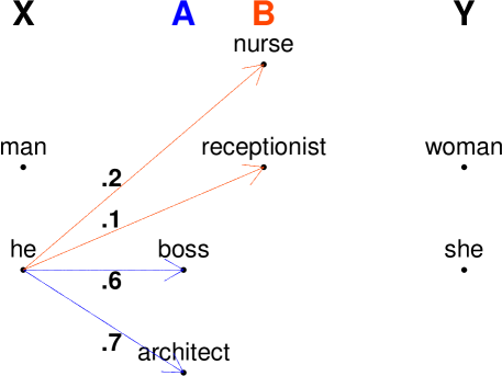
Figure 1: A simple example of a two-class set-up. Two groups of protected words, $X$ and $Y$ with two stereotypical attribute sets. An example of WEAT calculations follows.

Here is an example of WEAT calculations for Figure 1:

$$s_{1} =s(he,A,B)=\nicefrac{{(.6+.7)}}{{2}}-\nicefrac{{(.2+.1)}}{{2}}=.65-.15=.5$$

$$s_{2} =s(man,A,B)=.3$$

$$s_{3} =s(woman,A,B)=-.6$$

$$s_{4} =s(she,A,B)=-.3$$

$$\mathsf{WEAT}(A,B) =\frac{\nicefrac{{(s_{1}+s_{2})}}{{2}}-\nicefrac{{(s_{3}+s_{4})}}{{2}}}{sd(\{s_{1},s_{2},s_{3},s_{4}\})}\approx 1.93$$

WEAT has been developed to investigate biases corresponding to a pair of supposedly opposing stereotypes, so the question arises as to how to generalize the measure to contexts in which biases with respect to more than two stereotypical groups are to be measured. Such a generalization can be found in [13]. The authors introduce Mean Average Cosine distance (MAC) as a measure of bias. Let $T=\{t_{1},\dots,t_{k}\}$ be a set of protected words, and let each $A_{j}\in\mathcal{A}$ be a set of attributes stereotypically associated with a protected word where $\mathcal{A}$. For instance, when biases related to religion are to be investigated, they use a dataset of the format illustrated in Table 1. The measure is defined as follows:

protected words ($T$)	attributes	attribute set ($A_{j}$)	cosine distance
rabbi	greedy	jewStereotype	1.03
church	familial	christianStereotype	0.70
synagogue	liberal	jewStereotype	0.79
jew	familial	christianStereotype	0.98
quran	dirty	muslimStereotype	1.12
muslim	uneducated	muslimStereotype	0.52
torah	terrorist	muslimStereotype	0.93
quran	hairy	jewStereotype	1.18
synagogue	violent	muslimStereotype	0.95
bible	cheap	jewStereotype	1.22
christianity	greedy	jewStereotype	0.97
muslim	hairy	jewStereotype	0.88
islam	critical	christianStereotype	0.79
muslim	conservative	christianStereotype	0.45
mosque	greedy	jewStereotype	1.15

Table 1: Sample 15 rows of the religion dataset. The whole dataset has 15 unique protected words ($T$), and 11 unique attributes divided between 3 attribute sets ($A_{1}=\mathsf{jewStereotype},A_{2}=\mathsf{christianStereotype},A_{3}=\mathsf{muslimStereotype}$). $\mathcal{A}$ consists of these three sets, $\mathcal{A}=\{A_{1},A_{2},A_{3}\}$. The whole dataset has $15\times 11=165$ rows.

$$\mathsf{s}(t,A_{j}) =\frac{1}{|A_{j}|}\sum_{a\in A_{j}}\mathsf{cosineDistance}(t,a)$$

$$\mathsf{MAC}(T,\mathcal{A}) =\frac{1}{|T|\,|\mathcal{A}|}\sum_{t\in T}\sum_{A_{j}\in\mathcal{A}}\mathsf{s}(t,A_{j})$$

That is, for each protected word $t\in T$, and each attribute set $A_{j}$, they first take the mean of distances for this protected word and all attributes in a given attribute class, and then take the mean of thus obtained means for all the protected words and all the protected classes.

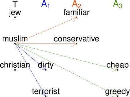
Figure 2: A small subset of the religion dataset. To each protected word in $T$ there corresponds one class of stereotypical attributes typically associated with it (and other classes of stereotypical attributes associated with different protected words).

An example of MAC calculations for the situation depicted in Figure 2 is as follows:

$$s_{1}=s(muslim,A_{1}) =\frac{\mathsf{cos}(muslim,dirty)+\mathsf{cos}(muslim,terrorist)}{2}$$

$$s_{2}=s(muslim,A_{2}) =\frac{\mathsf{cos}(muslim,familiar)+\mathsf{cos}(muslim,conservative)}{2}$$

$$\vdots$$

$$\mathsf{MAC}(T,A) =\mathsf{mean}(\{s_{i}|i\in 1,\dots,k\})$$

Notably, the intuitive distinction between different attribute sets plays no real role in the MAC calculations. Equally well one could calculate the mean distance of muslim to all the predicates, mean distance of christian to all the predicates, the mean distance of jew to all the predicates, and then to take the mean of these three means.

Having introduced the measures, first, we will introduce a selection of general problems with this approach, and then we will move on to more specific but important problems related to the fact that the measures take averages and averages of averages. Once this is done, we move to the development of our Bayesian alternative and the presentation of its deployment.

3 Challenges to cosine-based bias metrics

3.1 Interpretability issues

Table 2 contains an example of MAC scores (and $p$ values, we explain how these are obtained in Subsection 3.2) before and after deploying two debiasing methods to the Reddit embedding, where the score is calculated using the Religion word lists from [13]. For our purpose the details of the debiasing method are not important: what matters is that MAC is used in the evaluation of these methods.

Religion Debiasing	MAC	a p-value
Biased	0.859	N/A
Hard Debiased	0.934	3.006e-07
Soft Debiased ($\lambda$ = 0.2)	0.894	0.007

Table 2: The associated mean average cosine similarity (MAC) and p-values for debiasing methods for religious bias.

The first question we should ask is whether the initial MAC values lower than 1 indeed are indicative of the presence of bias? Thinking abstractly, 1 is the ideal distance for unrelated words. But in fact, there is some variation in distances, which might lead to non-biased lists also having MAC scores smaller than 1. How much smaller? What may attract attention is the fact that the value of cosine distance in “Biased” category is already quite high (i.e. close to 1) even before debiasing. High cosine distance indicates low cosine similarity between values. One could think that the average cosine similarity equal to approximately 0.141 is not large enough to claim the presence of a bias to start with. The authors, though, still aim to mitigate it by making the distances involved in the MAC calculations even larger. The question is, on what basis is this small similarity still considered as proof of the presence of bias, and whether these small changes are meaningful.

The problem is that the original paper did not employ any control group of neutral attributes for comparison to obtain a more realistic gauge on how to understand MAC values. Later on, in our approach, we introduce such control word lists. One of them is a list of words we intuitively considered neutral. Moreover, it might be the case that words that have to do with human activities in general, even if unbiased, are systematically closer to the protected words than merely neutral words. This, again, casts doubt on whether comparing MAC to the abstractly ideal value of 1 is a methodologically sound idea. For this reason, we also use a second list with intuitively non-stereotypical human attributes.

Another important observation is that MAC calculations do not distinguish whether a given attribute is associated with a given protected word, simply averaging across all such groups. Let us use the case of religion-related stereotypes to illustrate. The full lists from [13] can be found in Appendix A.3.1. In the original paper, words from all three religions were compared against all of the stereotypes. No distinction between cases in which the stereotype is associated with a given religion, as opposed to the situation in which it is associated with another one, is made. For example, the protected word jew is supposed to be stereotypically connected with the attribute greedy, while from the protected word quran the attribute greedy comes from a different stereotype, and yet the distances between these pairs contribute equally to the final MAC score. This is problematic, as not all of the stereotypical words have to be considered harmful for all religions. To avoid the masking effect, one should pay attention to how protected words and attributes are paired with stereotypes.

In Figures (3-5) we look at the empirical distributions, while paying attention to such divisions. The horizontal lines represent the values of $1-\mathsf{MAC}$ (that is, we now talk in terms of cosine similarity rather than cosine distance) that the authors considered indicative of bias for stereotypes corresponding to given word lists. For instance, in religion, MAC was .859, which was considered a sign of bias, so we plot $0\pm(1-.859)\approx.14$ lines around similarity = 0 (that is, distance = 1). Notice that most distributions are quite wide, and the proportions of even neutral or human neutral words with similarities higher than the value of $1-\mathsf{MAC}$ deserving debiasing according to the authors are quite high.

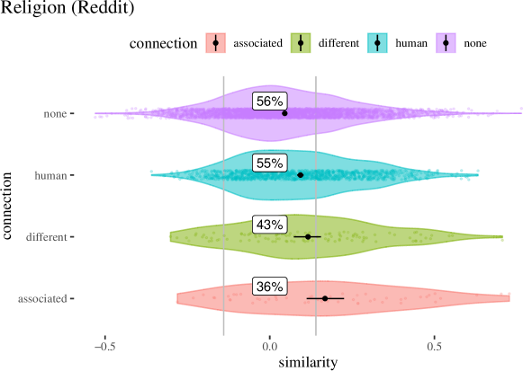
Figure 3: Empirical distributions of cosine similarities for the Religion word list used in the original paper.

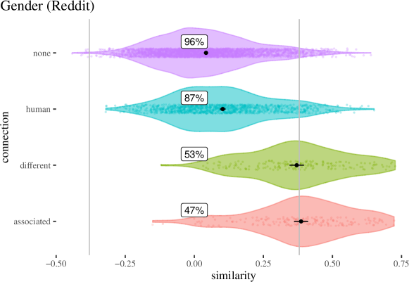
Figure 4: Empirical distributions of cosine similarities for the Gender word list used in the original paper.

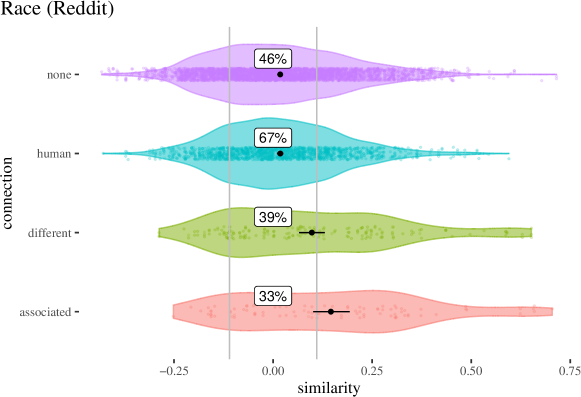
Figure 5: Empirical distributions of cosine similarities for the Race word list used in the original paper.

Another issue to consider is the selection of attributes for bias measurement. The word lists used in the literature are often fairly small (5-50). The papers in the field do employ statistical tests to measure the uncertainty involved and do make claims of statistical significance. Yet, we will later on argue that these method are not proper for the goal at hand. By using Bayesian methods we will show that a more appropriate use of statistical methods leads to estimates of uncertainty which suggest that larger word lists would be advisable.

To avoid the problem brought up in this subsection, we employ control groups and in line with Bayesian methodology, use posterior distributions and highest posterior density intervals instead of chasing single-point metrics based on pre-averaged data. Before we do so, we first explain why pre-averaging and chasing single-number metrics is a sub-optimal strategy.

3.2 Problems with pre-averaging

The approaches we have been describing use means of mean average cosine similarities to measure similarity between protected words and attributes coming from harmful stereotypes. But once we take a look at the individual values, it turns out that the raw data variance is rather high, and there are quite a few outliers and surprisingly dissimilar words. This problem becomes transparent when we examine the visualizations of the individual cosine distances, following the idea that one of the first steps in understanding data is to look at it. Let’s start with inspecting two examples of such visualizations in Figures 6 and 7 (we also include neutral and human predicates to make our point more transparent). Again, we emphasize that we do not condone the associations which we are about to illustrate.

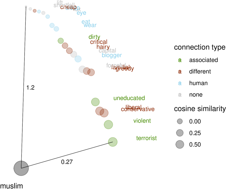
Figure 6: Actual distances for the protected word muslim.

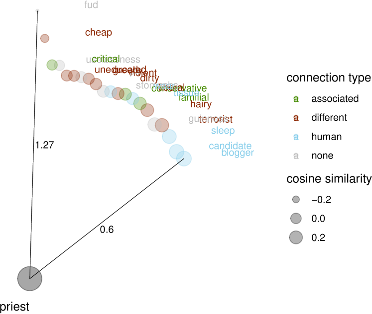
Figure 7: Actual distances for the protected word priest.

As transparent in Figures 6 and 7, for the protected word muslim, the most similar attributes tend to be the ones associated with it stereotypically, but then words associated with other stereotypes come closer than neutral or human predicates. For the protected word priest, the situation is even less as expected: the nearest attributes are human attributes, and all there seems to be no clear pattern to the distances to other attributes.

The general phenomenon that makes us skeptical about running statistical tests on pre-averaged data is that raw datasets of different variance can result in the same pre-averaged data and consequently the same single-number metric. In other words, a method that proceeds this way is not very sensitive to the real sample variance.

Let us illustrate how this problem arises in the context of WEAT. Once a particular $s(X,Y,A,B)$ is calculated, the question arises as to whether a value that high could have arisen by chance. To address the question, each $s(X,Y,A,B)$ is used in the original paper to generate a $p$-value by bootstrapping. The $p$-value is the frequency of how often it is the case that $s(X_{i},Y_{i},A,B)>s(X,Y,A,B)$ for sampled equally sized partitions $X_{i},Y_{i}$ of $X\cup Y$. The WEAT score is then computed by standardizing the difference in means of means by dividing by the standard deviation of means, see equation (3).

The WEAT scores reported by [9] for lists of words for which the embeddings are supposedly biased range from 2.06 to 1.81, and the reported $p$-values are in the range of $10^{-7}-10^{-2}$ with one exception for Math vs Arts, where it is $.018$.

The question is, are those results meaningful? One way to answer this question is to think in terms of null generative models. If the words actually are samples from two populations with equal means, how often would we see WEAT scores in this range? How often would we reach the $p$-values that the authors reported?

Imagine there are two groups of protected words, each of size 8, and two groups of stereotypical attributes, of the same size. Each such a collection of samples, as far as our question is involved, is equivalent to a sample of $16^{2}$ cosine distances. Further, imagine there really is no difference between these groups of words and the model is in fact null. That is, we draw the cosine distances from the $\mathsf{Normal}(0,.08)$ distribution.

In Figure 8 we illustrate one iteration of the procedure. We draw one such sample of size $16^{2}$. Then we actually list all possible ways to split the 16 words in two equal sets (each such a split is one bootstrapped sample) and for each of them we calculate the s values and WEAT. What are the resulting distributions of s scores and what $p$-values do they lead to? What are the resulting effect sizes for each bootstrapped sample, and how often can we get an effect size as large as the ones reported in the original paper?

In the bootstrapped samples we would rather expect low s values and low WEAT: after all, these are just random permutations of random distances all of which are drawn from the same null distribution. Let’s take a look at one such a bootstrapped sample.

On purpose, we picked a rather unusual one: the observed test statistic is 0.39 and 1.27. The bootstrapped distributions of the test statistics and effect sizes are illustrated in Figure 8, together with this particular example. Quite notably both (two-sided) $p$ values for our example are rather low (Figure 8). These facts might suggest that we ended up with a situation where “bias” is present (albeit, due to random noise). The reason why we picked it is that it is an example of a word list that ends up with relatively low $p$-value and a relatively unusual effect size, but nevertheless, its closer inspection shows that even for a word list with such properties there is no clear reason to think that the bias is present.

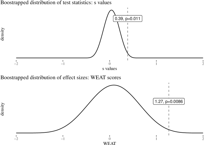
Figure 8: Bootstrapped distributions of test statistics and effect sizes in a random sample given the null hypothesis. We used a sample from the null model with N(0,.08) and 16 protected words, and then bootstrapped from it, following the original methodology. One particular bootstrapped sample is highlighted, and discussed further in the text.

At this point, we might think that we just stumbled into a bootstrapped sample that randomly happened to display strong bias. We decide to double-check this by visual inspection expecting exactly this: a strong, clearly visible bias (Figure 9).

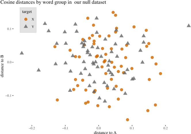
Figure 9: Cosine distances to two attribute sets by protected word groups. Observe nothing unusual except for a few outliers.

In fact, while there might be some outliers here and there, saying that a clear bias on which one group is systematically closer to $A$s than another is definitely a stretch. What happened?

In the calculations of WEAT means are taken twice. The s-values themselves are means and then means of s-values are compared between groups. Statistical troubles start when we run statistical tests on sets of means, for at least two reasons.

1. By pre-averaging data we throw away information about sample sizes. For the former point, think about proportions: 10 out of 20 and 2 out of 4 give the same mean, but you would obtain more information by making the former observation rather than by making the latter. And especially in this context, in which the word lists are not huge, sample sizes should matter.

2. When we pre-average, we disregard variation, and therefore pre-averaging tends to manufacture false confidence. Group means display less variation than the raw data points and the standard deviation of a set of means of sets of means is bound to be lower than the original standard deviation in the row data. Now, if you calculate your effect size by dividing by the pre-averaged standard deviation, you are quite likely to get something that looks like a strong effect size, but the results of your calculations might not track anything interesting.

Let us think again about the question that we are ultimately interested in. Are the $X$ terms systematically closer to (further from) the $A$ attributes ($B$ attributes) than the $Y$ words? But now let’s use the raw data points to try to answer these questions.

To start with, let us run two quick $t$-tests to gauge what the raw data illustrated in Figure 9 tell us. First, distances to $A$ attributes for $X$ words and $Y$ words. Well, the result is—strictly speaking—statistically significant. The $p$-value is $0.02$ (more than ten times higher than the $p$-valued obtained by the bootstrapping procedure. So the sample is in some sense unusual. But the 95% confidence interval for the difference in means is $[.0052,.061]$, clearly nothing that a reader would expect given that the calculated effect size seemed quite large. How about the distances to the $B$ attributes? Here the $p$-value is $.22$ and the 95% confidence interval is $[-0.03,.009]$, even less of a reason to think a bias is present.

The difficulties are exacerbated by the fact that statistical tests are based on bootstrapping from a relatively small data sets, which is quite likely to underestimate the population variance. To make our point clear, let us avoid bootstrapping and work with the null generative model with $\mathsf{Norm}(0,.08)$ for both word groups. We keep the sizes the same: we have eight protected words in each group, sixteen in total, and for each we randomly draw 8 distances from hypothetical $A$ attributes, and $8$ distances from hypothetical $B$ attributes. Calculate the test statistic and effect size the way [9] did. Do this 10000 times, each time calculating WEAT and s values, and look at what the distributions of these values are on the assumption of the null model with realistic empirically motivated raw data point standard deviation.

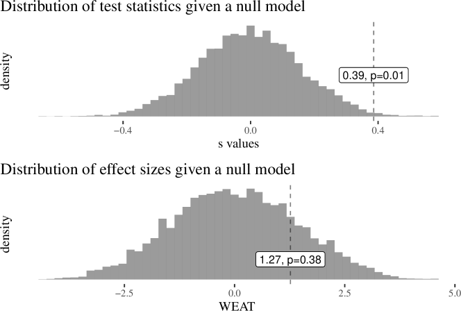
Figure 10: Distributions of test statistics and effect sizes based on 10k simulations on the assumption of a null model in which all distances come from normal distribution with $\mu=0,\sigma=.08,n=10k$. We also mark the sample we have been using as an example.

The first observation is that the supposedly large effect size we obtained is not that unusual even assuming a null model. Around 38% of samples result in WEAT score at least as extreme. This illustrates the point that it does not constitute a strong evidence of bias. Second, the distribution of s values is much more narrow, which means that if we use it to calculate $p$-values, it is not too difficult to obtain a supposedly significant test statistic which nevertheless does not correspond to anything interesting happening in the data set.

We have seen that seemingly high effect sizes might arise even if the underlying processes actually have the same mean. The uncertainty resulting from including the raw data point variance in considerations is more extensive than the one suggested by the low $p$-values obtained from taking means or means of means as data points. In the section we discussed the performance of the WEAT measure, but since the [13] one is a generalization thereof, including the method of running statistical tests on pre-averaged data, our remarks, mutatis nutandis, apply.

What is the alternative? As we already emphasized: focusing on what the real underlying question is and trying to answer it using a statistical analysis of the raw data using meaningful control groups, to ensure interpretability. Moreover, since the data sets are not too large and since multiple evaluations are to be made, we will pursue this method from the Bayesian perspective. Now we have to describe it.

4 A Bayesian approach to cosine-based bias

4.1 Model construction

Bayesian data analysis takes prior probability distributions, a mathematical model structure and the data, and returns the posterior probability distributions over the parameters of interest, thus capturing our uncertainty about their actual values. One important difference between such a result and the result of classical statistical analysis is that classical confidence intervals (CIs) have a rather complicated and somewhat confusing interpretation, which has little to do with the posterior probability distribution.

In fact, Bayesian highest posterior density intervals (HPDIs, the narrowest intervals containing a certain ratio of the area under the curve) and CIs end up being numerically the same only if the prior probabilities are uniform. This illustrates that (1) classical analysis is unable to incorporate non-trivial priors, and (2) is therefore more susceptible to over-fitting, unless regularization (equivalent to a more straightforward Bayesian approach) is used. In contrast with CIs, the posterior distributions are easily interpretable and have direct relevance to the question at hand. Moreover, Bayesian data analysis is better at handling hierarchical models and small datasets, which is exactly what we will we dealing with.

In standard Bayesian analysis, the first step is to understand the data, think hard about the underlying process, and select potential predictors and the outcome variable. The next step is to formulate a mathematical description of the generative model of the relationships between the predictors and the outcome variable. Prior distributions must then be chosen for the parameters used in the model. Next, Bayesian inference must be applied to find posterior distributions over the possible parameter values. Finally, we need to check how well the posterior predictions reflect the data with a posterior predictive check.

In our analysis, the outcome variable is the cosine distances between the protected words and attribute words. The predictor is a factor determining whether a given attribute word is a neutral word, a human predicate is stereotypically associated with the protected word, or comes from a different stereotype connected with another protected word. The idea is really straightforward: if bias is present in the embedding, distances to associated attribute words should be systematically lower than to other attribute words.

Furthermore, conceptually there are two levels of analysis in our approach (see Figure 11). On the one hand, we are interested in the general question of whether related attributes are systematically closer across the dataset. On the other hand, we are interested in a more fine-grained picture of the role of the predictor for particular protected words. Learning in hierarchical Bayesian models involves using Bayesian inference to update the parameters of the model. This update is based on the observed data, and estimates are made at different levels of the data hierarchy. We use hierarchical Bayesian models in which we simultaneously estimate parameters at the protected word level and at the global level, assuming that all lower-level parameters are drawn from global distributions. Such models can be thought of as incorporating adaptive regularization, which avoids overfitting and leads to improved estimates for unbalanced datasets (and the datasets we need to use are unbalanced).

Figure 11: At a general level, we will be estimating the coefficients for distances as grouped by whether they are between protected words and attributes coming from their respective associated/different/human/neutral attribute groups. At a more fine-grained level, for each protected word we will be estimating the proximity of that word to attributes that are associated with its respective stereotype, come from a different stereotype, or come from the human/neutral attribute lists.

To be more specific, the underlying mathematical model is as follows. First, we assume that distances are normally distributed:

$$\mathsf{distance_{i}} \sim\mathsf{dnorm}(\mu_{i},\sigma_{i})$$

Second, for each particular protected word $\mathsf{pw}$ there are four parameters to be estimated. Its mean distance to associated stereotypes $a[pw]$, its mean distance to attributes coming from different stereotypes, $d[pw]$, its mean distance to human attributes, $h[pw]$, and its mean distance to neutral attributes, $n[pw]$:

$$\mu_{i} =d_{\mathsf{pw[i]}}\times\mathsf{different}_{i}+a_{\mathsf{pw[i]}}\times\mathsf{associated}_{i}+h_{\mathsf{pw[i]}}\times\mathsf{human}_{i}+n_{\mathsf{pw[i]}}\times\mathsf{neutral}_{i}$$

where $\mathsf{different},\mathsf{associated},\mathsf{human}$ and $\mathsf{neutral}$ are binary variables. This completes our description of the simple underlying process that we would like to investigate.

Now the priors and the hierarchy. We assume all the $a$ parameters come from one distribution, that is normal around a higher-level parameter $\bar{a}$ and so on for the other three groups of parameters. That is, $a_{\mathsf{pw[i]}}$ is the average distance of a given particular protected word to attributes stereotypically associated with it, while $\bar{a}$ is the overall average distance of protected words to attributes associated with them.

$$d_{\mathsf{pw[i]}}\sim\mathsf{Norm}(\bar{d},\overline{\sigma_{d}}) a_{\mathsf{pw[i]}}\sim\mathsf{Norm}(\bar{a},\overline{\sigma_{a}})$$

$$h_{\mathsf{pw[i]}}\sim\mathsf{Norm}(\bar{h},\overline{\sigma_{h}}) n_{\mathsf{pw[i]}}\sim\mathsf{Norm}(\bar{n},\overline{\sigma_{n}})$$

According to our priors, the group means $\bar{a}$, $\bar{d}$, $\bar{h}$ and $\bar{n}$ all come from one normal distribution with mean equal to $1$ and standard deviation equal to $.3$. The standard deviations $\bar{\sigma_{a}}$, $\bar{\sigma_{d}}$, $\bar{\sigma_{h}}$ and $\bar{\sigma_{n}}$ to be estimated, according to our prior, come from one distribution, exponential with rate parameter equal to $2$. Our priors are slightly skeptical. They do reflect our knowledge and intuition on the probable distribution of the cosine distances in the data. We know that the cosine distances lie in the range $0-2$, and we expect two randomly chosen vectors from the embedding to have rather small similarity, so we expect the distances to be centered around $1$. However, we use a rather wide standard deviation ($.3$) to easily account for cases where there is actually much higher similarity between two vectors (especially in cases where the embedding is supposed to be biased). Our priors for the standard deviations are also fairly weak.

$$\bar{d},\bar{a},\bar{h},\bar{n} \sim\mathsf{Norm}(1,.3)$$

$$\overline{\sigma_{d}},\overline{\sigma_{a}},\overline{\sigma_{h}},\overline{\sigma_{n}} \sim\mathsf{Exp}(2)$$

4.2 Posterior predictive check

A posterior predictive check is a technique used to evaluate the fit of a Bayesian model by comparing its predictions with observed data. The underlying principle is to generate simulated data from the posterior distribution of the model parameters and compare them with the observed data. If the model is a good fit to the data, the simulated data should resemble the observed data. In Figure 12 we illustrate a posterior predictive check for one corpus (Reddit) and one word list. The remaining posterior predictive checks are in section A.2.

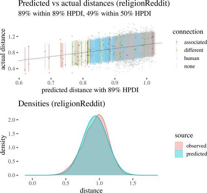
Figure 12: Example of a posterior predictive check. (Top) Actual cosine distances are plotted against mean predictions with 89% highest posterior density intervals. Notice that 90% of actual values fall within the 89% HPDI and 55% of actual values fall into 50% HPDI, which indicates appropriate performance of the model. The left-right alignment of different colors corresponds to the fact that cosine differences between elements of different categories differ, to some extent systematically (this will be studied in the results section). (Bottom) Densities of predicted and observed distances.

5 Results and discussion

5.1 Observations

In brief, despite one-number metrics suggesting otherwise, our Bayesian analysis reveals that insofar as the short word lists usually used in related research projects are involved, there usually are no strong reasons to claim the presence of systematic bias. Moreover, comparison between the groups (including control word lists) leads to the conclusion that the effect sizes (that is, the absolute differences between cosine distances between groups) tend to be rather small, with few exceptions. Moreover, the choice of protected words is crucial — as there is a lot of variance when it comes to the protected word-level analysis.

In a bit more detail, the visualizations in Appendix A.1 show that the situation is more complicated than merely looking at one-number summaries might suggest. Note that the axes are sometimes in different scales to increase visibility.

To start with, let us look at the association-type level coefficients (illustrated in the top parts of the plots). Depending on the corpus used and word class, there is a large variety as to posterior densities. Quite aware of this being a crude approximation, let’s compare the HPDIs and whether they overlap for different attribute groups.

• In Weat 7 (Reddit) there is no reason to think there are systematic differences between cosine distances (recall that words from Weat 7 were mostly not available in other embeddings).

• In Weat 1 (Google, Glove and Reddit) associated words are somewhat closer, but the cosine distance differences from neutral words are very low, and surprisingly it is human attributes, not neutral predicates that are systematically the furthest.

• In Religion (Google, Glove, Reddit) and Race (Google, Glove), the associated attributes are not systematically closer than attributes belonging to different stereotypes, and the difference between neutral and human predicates is rather low, if noticeable. The situation is interestingly different in Race (Reddit) where both human and neutral predicates are systematically further than associated and different attributes—but even then, there is no clear difference between associated and different attributes.

• For Gender (Google, Glove), despite the superficially binary nature, associated and opposite attributes tend to be more or less in the same distances, much closer than neutral words (but not closer than human predicates in Glove). Reddit is an extreme example: both associated and opposite attributes are much closer than neutral and human (around .6 vs. .9), but even then, there seems to be no reason to think that cosine distances to associated predicates are much different from distances to opposite predicates.

Moreover, when we look at particular protected words, the situation is even less straightforward. We will just go over a few notable examples, leaving the visual inspection of particular results for other protected words to the reader. One general phenomenon is that—as we already pointed out—the word lists are quite short, which contributes to large uncertainty involved in some cases.

• For some protected words the different attributes are somewhat closer than the associated attributes.

• For some protected words, associated and different attributes are closer than neutral attributes, but so are human attributes.

• In some cases, associated attributes are closer, but so are neutral and human predicates, which illustrates that just looking at average cosine similarity as compared to the theoretically expected value of 1, instead of running a comparison to neutral and human attributes is misleading.

• The only group of protected words where differences are noticeable at the protected word level is Gender-related words– as in Gender (Google) and in Gender (Reddit) — note however that in the latter, for some words, the opposite attributes seem to be a little bit closer than the associated ones.

5.2 Rethinking debiasing

Bayesian analyses and visualizations thereof can be also handy when it comes to the investigation of the effect that debiasing has on the embedding space. In Figures 13 and 14 we see an example of two visualizations depicting the difference in means with 89% highest posterior density intervals before and after applying debiasing (the remaining visualizations are in the Appendix).

• In Gender (Reddit), minor differences between different and associated predicates end up being smaller. However, this is not achieved by any major change in the relative positions of associated and different predicates with respect to protected words, but rather by shifting them jointly together. The only protected word for which a major difference is noticeable is hers.

• In Religion (Reddit) debiasing aligns general coefficients for all groups together, all of them getting closer to where neutral words were prior to debiasing (this is true also for human predicates in general, which intuitively did not require debiasing). For some protected words such as christian, jew, the proximity ordering between associated and different predicates has been reversed, and most of the distances shifted a bit towards 1 (sometimes even beyond, such as predicates associated with the word quran), but for most protected words, the relative differences between the coefficient did not change much (for instance, there is no change in the way the protected word muslim is mistreated).

• For Race (Reddit), general coefficients for different and associated predicates became aligned. However, most of the changes roughly preserve the structure of bias for particular protected words with minor exceptions, such as making the proximities of different predicates for protected words asian and asia much lower than associated predicates, which is the main factor responsible for the alignment of the general level coefficients.

In general, debiasing might end up leading to lower differences between general level coefficients for associated and different attributes. But that usually happens without any major change to the structure of the coefficients for protected words, sporadic extreme and undesirable changes for some protected words, usually with the side-effect of changing what happens with neutral and human predicates.

We wouldn’t be even able to notice these phenomena had we restricted our attention to MAC or WEAT scores only. To be able to diagnose and remove biases at the right level of granularity, we need to go beyond single metric chasing.

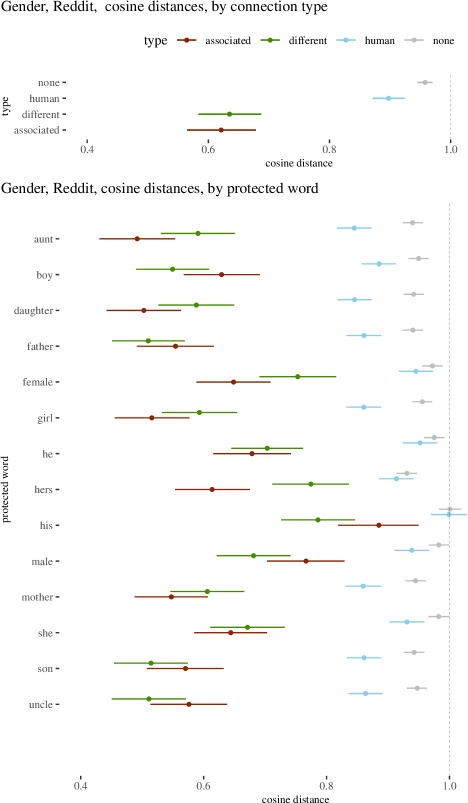
Figure 13: Mean cosine distances with 89% highest posterior density intervals for the gender dataset before debiasing.

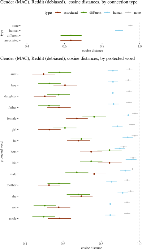
Figure 14: Mean with 89% highest posterior density intervals for gender after debiasing.

In Figures 15-17 we inspect the empirical distributions for the debiased embeddings. Comparing the results to the original embedding, one may notice that for the Religion group, the neutral and human distribution has changed slightly. Before within the “correct” cosine similarity boundaries, there were 56% of neutral and 55% of human word lists. After the debiasing, the values changed to 59% (for neutral) and 59% (for human). The different and associated word lists were more influenced. The general shape of both distributions is less stretched. Before debiasing 43% of the different word lists and 35% of the associated word lists were within the accepted boundaries. After the embedding manipulation, the percentage has increased for both lists to 63%. Visualization for Gender group illustrates almost no change for the neutral and human word lists before and after debiasing. The values for different and associated word lists are also barely impacted by the embedding modification. In the Race group, the percentage within the boundaries for neutral and associated word lists has increased. The opposite happened for human and different word lists, where the percentage of “correct” cosine similarity dropped from 67% to 55% (human) and from 39% to 36% (different).

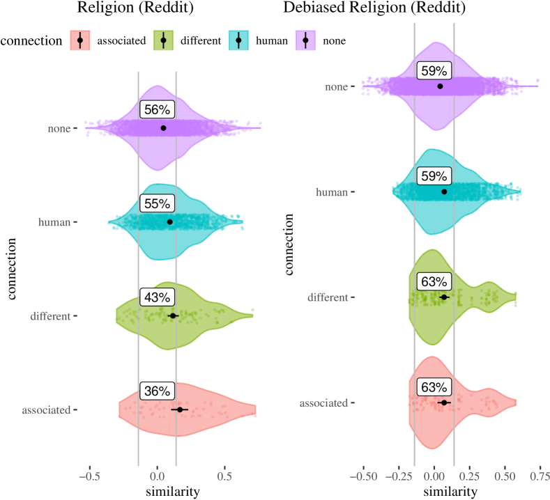
Figure 15: Empirical distributions of cosine similarities before and after debiasing for the Religion word list used in the original paper.

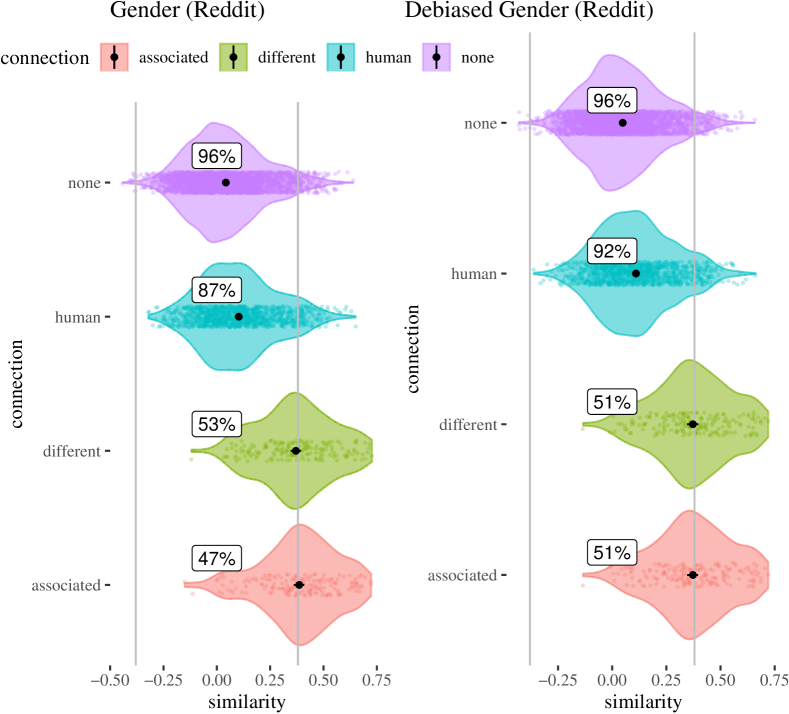
Figure 16: Empirical distributions of cosine similarities before and after debiasing for the Gender word list used in the original paper.

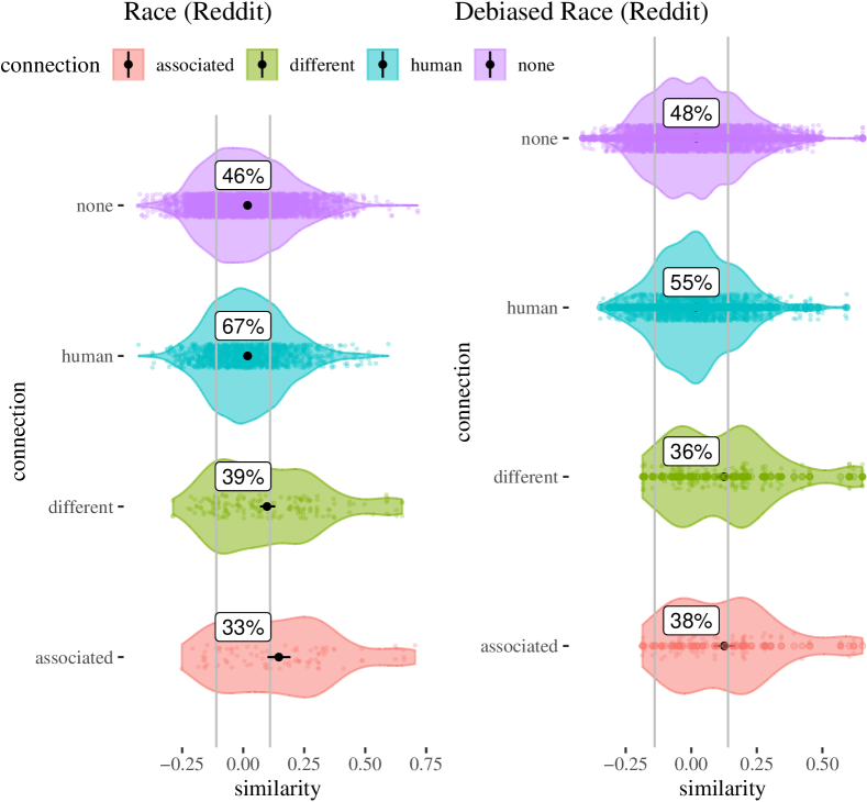
Figure 17: Empirical distributions of cosine similarities before and after debiasing for the Race word list used in the original paper.

6 Related works and conclusions

There are a few related papers, whose discussion goes beyond the scope of this paper:

• [21] employ Bayesian methods to estimate uncertainty in NLP tasks, but they apply their Bayesian Neural Networks-based method to sentiment analysis or named entity recognition, not to bias.

• [2] correctly argues that a bias estimate should not be expressed as a single number without taking into account that the estimate is made using a sample of data and therefore has intrinsic uncertainty. The authors suggest using Bernstein bounds to gauge the uncertainty in terms of confidence intervals. We do not discuss this approach extensively, as we think that confidence intervals are quite problematic for several reasons, among others the confusing interpretability. We do not think that Bernstein bounds provide the best solution to the problem. Applying this method to a popular WinoBias dataset leads to the conclusion that more than 11903 samples are needed to claim a 95% confidence interval for a bias estimate. This amount vastly exceeds the existing word lists for bias estimation. We propose a more realistic Bayesian method. Our conclusion is still that the word lists are sometimes too small, but at least they allow for gauging uncertainty as we go on to improve our methodology and extend the lists gradually.

• [20] criticize some existing bias metrics such as MAC or WEAT on the grounds of them not satisfying some general formal principles, such as magnitude-comparability, and they propose a modification, called SAME.

• [14] develop a generalization of WEAT meant to apply to sets of sentences, SEAT, which basically applies WEAT to vector representations of sentences. The authors, however, still pre-average and play the game of finding a single-number metric, so our remarks apply.

• [7] introduce the Contextualized Embedding Association Test Intersectional, meant to apply to dynamic word embeddings and, importantly develop methods for intersectional bias detection. The measure is a generalization of the WEAT method. The authors do inspect a distribution of effect sizes that arises from the consideration of various possible contexts, but they continue to standardize the difference in averaged means and use a single-number summary: the weighted mean of the effect sizes thus understood. The method, admittedly, deserves further evaluation which goes beyond the scope of this paper.

To summarize, a Bayesian data analysis with hierarchical models of cosine distances between protected words, control group words, and stereotypical attributes provides more modest and realistic assessment of the uncertainty involved. It reveals that much complexity is hidden when one instead chases single bias metrics present in the literature. After introducing the method, we applied it to multiple word embeddings and results of supposed debiasing, putting forward some general observations that are not exactly in line with the usual picture painted in terms of WEAT or MAC (and the problem generalizes to any approach that focuses on chasing a single numeric metric): the word list sizes and sample sizes used in the studies are usually small. Posterior density intervals are fairly wide. Often the differences between associated, different and neutral human predicates, are not very impressive. Also, a preliminary inspection suggests that the desirability of changes obtained by the usual debiasing methods is debatable. The tools that we propose, however, allow for a more fine-grained and multi-level evaluation of bias and debiasing in language models without losing modesty about the uncertainties involved. The short, general, and somewhat disappointing lesson here is this: things are complicated. Instead of chasing single-number metrics, we should rather devote attention to more nuanced analysis.

References

re [1] Tolga Bolukbasi, Kai-Wei Chang, James Y. Zou, Venkatesh Saligrama, and Adam Kalai. 2016. Man is to computer programmer as woman is to homemaker? Debiasing word embeddings. CoRR abs/1607.06520, (2016). Retrieved from http://arxiv.org/abs/1607.06520

pre [2] Kawin Ethayarajh. 2020. Is your classifier actually biased? Measuring fairness under uncertainty with bernstein bounds. CoRR abs/2004.12332, (2020). Retrieved from https://arxiv.org/abs/2004.12332

pre [3] Nikhil Garg, Londa Schiebinger, Dan Jurafsky, and James Zou. 2017. Word embeddings quantify 100 years of gender and ethnic stereotypes. Proceedings of the National Academy of Sciences 115, (November 2017). DOI:https://doi.org/10.1073/pnas.1720347115

pre [4] Nikhil Garg, Londa Schiebinger, Dan Jurafsky, and James Zou. 2018. Word embeddings quantify 100 years of gender and ethnic stereotypes. Proceedings of the National Academy of Sciences 115, 16 (April 2018), E3635–E3644. DOI:https://doi.org/10.1073/pnas.1720347115

pre [5] Hila Gonen and Yoav Goldberg. 2019. Lipstick on a pig: Debiasing methods cover up systematic gender biases in word embeddings but do not remove them. In Proceedings of the 2019 conference of the north American chapter of the association for computational linguistics: Human language technologies, volume 1 (long and short papers), Association for Computational Linguistics, Minneapolis, Minnesota, 609–614. DOI:https://doi.org/10.18653/v1/N19-1061

pre [6] Jonathan Gordon and Benjamin Durme. 2013. Reporting bias and knowledge acquisition. In AKBC 2013 - Proceedings of the 2013 Workshop on Automated Knowledge Base Construction, Co-located with CIKM 2013, 25–30. DOI:https://doi.org/10.1145/2509558.2509563

pre [7] Wei Guo and Aylin Caliskan. 2021. Detecting emergent intersectional biases: Contextualized word embeddings contain a distribution of human-like biases. In Proceedings of the 2021 AAAI/ACM conference on AI, ethics, and society, ACM. DOI:https://doi.org/10.1145/3461702.3462536

pre [8] Rink Hoekstra, Richard D. Morey, Jeffrey N. Rouder, and Eric-Jan Wagenmakers. 2014. Robust misinterpretation of confidence intervals. Psychonomic Bulletin & Review 21, 5 (October 2014), 1157–1164. DOI:https://doi.org/10.3758/s13423-013-0572-3

pre [9] Aylin Caliskan Islam, Joanna J. Bryson, and Arvind Narayanan. 2016. Semantics derived automatically from language corpora necessarily contain human biases. CoRR abs/1608.07187, (2016). Retrieved from http://arxiv.org/abs/1608.07187

pre [10] Gabbrielle Johnson. forthcoming. Are algorithms value-free? Feminist theoretical virtues in machine learning. Journal Moral Philosophy (forthcoming).

pre [11] John Kruschke. 2015. Doing bayesian data analysis (second edition). Academic Press, Boston.

pre [12] Anne Lauscher and Goran Glavas. 2019. Are we consistently biased? Multidimensional analysis of biases in distributional word vectors. CoRR abs/1904.11783, (2019). Retrieved from http://arxiv.org/abs/1904.11783

pre [13] Thomas Manzini, Yao Chong Lim, Yulia Tsvetkov, and Alan W Black. 2019. Black is to criminal as caucasian is to police: Detecting and removing multiclass bias in word embeddings. Retrieved from https://arxiv.org/abs/1904.04047

pre [14] Chandler May, Alex Wang, Shikha Bordia, Samuel R. Bowman, and Rachel Rudinger. 2019. On measuring social biases in sentence encoders. In Proceedings of the 2019 conference of the north American chapter of the association for computational linguistics: Human language technologies, volume 1 (long and short papers), Association for Computational Linguistics, Minneapolis, Minnesota, 622–628. DOI:https://doi.org/10.18653/v1/N19-1063

pre [15] Richard McElreath. 2020. Statistical rethinking: A bayesian course with examples in r and stan, 2nd edition (2nd ed.). CRC Press. Retrieved from http://xcelab.net/rm/statistical-rethinking/

pre [16] Tomas Mikolov, Kai Chen, Greg Corrado, and Jeffrey Dean. 2013. Efficient estimation of word representations in vector space. DOI:https://doi.org/10.48550/ARXIV.1301.3781

pre [17] Richard Morey, Rink Hoekstra, Jeffrey Rouder, Michael Lee, and EJ Wagenmakers. 2015. The fallacy of placing confidence in confidence intervals. Psychonomic Bulletin & Review (September 2015).

pre [18] Malvina Nissim, Rik van Noord, and Rob van der Goot. 2020. Fair is better than sensational: Man is to doctor as woman is to doctor. Computational Linguistics 46, 2 (June 2020), 487–497. DOI:https://doi.org/10.1162/coli_a_00379

pre [19] Brian A. Nosek, Mahzarin R. Banaji, and Anthony G. Greenwald. 2002. Harvesting implicit group attitudes and beliefs from a demonstration web site. Group Dynamics: Theory, Research, and Practice 6, 1 (2002), 101–115. DOI:https://doi.org/10.1037/1089-2699.6.1.101

pre [20] Sarah Schröder, Alexander Schulz, Philip Kenneweg, Robert Feldhans, Fabian Hinder, and Barbara Hammer. 2021. Evaluating metrics for bias in word embeddings. Retrieved from https://arxiv.org/abs/2111.07864

pre [21] Yijun Xiao and William Yang Wang. 2018. Quantifying uncertainties in natural language processing tasks. CoRR abs/1811.07253, (2018). Retrieved from http://arxiv.org/abs/1811.07253

p

Appendix A Appendix

A.1 Visualizations

A.2 Posterior predictive checks

A.3 Word lists

A.3.1 Lists used in previous research

The lists from [13] are available here:

• Gender: https://github.com/TManzini/DebiasMulticlassWordEmbedding/blob/master/Debiasing/data/vocab/gender_attributes_optm.json

• Race: https://github.com/TManzini/DebiasMulticlassWordEmbedding/blob/master/Debiasing/data/vocab/race_attributes_optm.json

• Religion: https://github.com/TManzini/DebiasMulticlassWordEmbedding/blob/master/Debiasing/data/vocab/religion_attributes_optm.json

The lists are:

• Gender:

Pairs of protected attributes: [“he”, “she”], [“his”, “hers”], [“son”, “daughter”], [“father”, “mother”], [“male”, “female”], [“boy”, “girl”], [“uncle”, “aunt”]

Lists of stereotypes per gender: man: [“manager”, “executive”, “doctor”, “lawyer”, “programmer”, “scientist”, “soldier”, “supervisor”, “rancher”, “janitor”, “firefighter”, “officer”], woman: [“secretary”, “nurse”, “clerk”, “artist”, “homemaker”, “dancer”, “singer”, “librarian”, “maid”, “hairdresser”, “stylist”, “receptionist”, “counselor”] }

• Race:

Sets of protected attributes: [“black”, “caucasian”, “asian”], [“african”, “caucasian”, “asian”], [“black”, “white”, “asian”], [“africa”, “america”, “asia”], [“africa”, “america”, “china”], [“africa”, “europe”, “asia”]

Lists of stereotypes per race: “caucasian”: [“manager”, “executive”, “redneck”, “hillbilly”, “leader”, “farmer”], “asian” : [“doctor”, “engineer”, “laborer”, “teacher”], “black” : [“slave”, “musician”, “runner”, “criminal”, “homeless”]

• Religion:

Sets of protected attributes: [“judaism”, “christianity”, “islam”], [“jew”, “christian”, “muslim”], [“synagogue”, “church”, “mosque”], [“torah”, “bible”, “quran”], [“rabbi”, “priest”, “imam”]

Lists of stereotypes per race: “jew” : [“greedy”, “cheap”, “hairy”, “liberal”], “christian” : [“judgemental”, “conservative”, “familial”], “muslim” : [“violent”, “terrorist”, “dirty”, “uneducated”]

A.3.2 Custom lists used in this paper

• Neutral:

[‘ballpark’, ‘glitchy’, ‘billy’, ‘dallas’, ‘rip’, ‘called’, ‘outlooks’, ‘floater’, ‘rattlesnake’, ‘exports’, ‘recursion’, ‘shortfall’, ‘corrected’, ‘solutions’, ‘diagnostic’, ‘patently’, ‘flops’, ‘approx’, ‘percents’, ‘lox’, ‘hamburger’, ‘engulfed’, ‘households’, ‘north’, ‘playtest’, ‘replayability’, ‘glottal’, ‘parable’, ‘gingers’, ‘anachronism’, ‘organizing’, ‘reach’, ‘shtick’, ‘eleventh’, ‘cpu’, ‘ranked’, ‘irreversibly’, ‘ponce’, ‘velociraptor’, ‘defects’, ‘puzzle’, ‘smasher’, ‘northside’, ‘heft’, ‘observation’, ‘rectum’, ‘mystical’, ‘telltale’, ‘remnants’, ‘inquiry’, ‘indisputable’, ‘boatload’, ‘lessening’, ‘uselessness’, ‘observes’, ‘fictitious’, ‘repatriation’, ‘duh’, ‘attic’, ‘schilling’, ‘charges’, ‘chatter’, ‘pad’, ‘smurfing’, ‘worthiness’, ‘definitive’, ‘neat’, ‘homogenized’, ‘lexicon’, ‘nationalized’, ‘earpiece’, ‘specializations’, ‘lapse’, ‘concludes’, ‘weaving’, ‘apprentices’, ‘fri’, ‘militias’, ‘inscriptions’, ‘gouda’, ‘lift’, ‘laboring’, ‘adaptive’, ‘lecture’, ‘hogging’, ‘thorne’, ‘fud’, ‘skews’, ‘epistles’, ‘tagging’, ‘crud’, ‘two’, ‘rebalanced’, ‘payroll’, ‘damned’, ‘approve’, ‘reason’, ‘formally’, ‘releasing’, ‘muddled’, ‘mineral’, ‘shied’, ‘capital’, ‘nodded’, ‘escrow’, ‘disconnecting’, ‘marshals’, ‘winamp’, ‘forceful’, ‘lowes’, ‘sip’, ‘pencils’, ‘stomachs’, ‘goff’, ‘cg’, ‘backyard’, ‘uprooting’, ‘merging’, ‘helpful’, ‘eid’, ‘trenchcoat’, ‘airlift’, ‘frothing’, ‘pulls’, ‘volta’, ‘guinness’, ‘viewership’, ‘eruption’, ‘peeves’, ‘goat’, ‘goofy’, ‘disbanding’, ‘relented’, ‘ratings’, ‘disputed’, ‘vitamins’, ‘singled’, ‘hydroxide’, ‘telegraphed’, ‘mercantile’, ‘headache’, ‘muppets’, ‘petal’, ‘arrange’, ‘donovan’, ‘scrutinized’, ‘spoil’, ‘examiner’, ‘ironed’, ‘maia’, ‘condensation’, ‘receipt’, ‘solider’, ‘tattooing’, ‘encoded’, ‘compartmentalize’, ‘lain’, ‘gov’, ‘printers’, ‘hiked’, ‘resentment’, ‘revisionism’, ‘tavern’, ‘backpacking’, ‘pestering’, ‘acknowledges’, ‘testimonies’, ‘parlance’, ‘hallucinate’, ‘speeches’, ‘engaging’, ‘solder’, ‘perceptive’, ‘microbiology’, ‘reconnaissance’, ‘garlic’, ‘neutrals’, ‘width’, ‘literaly’, ‘guild’, ‘despicable’, ‘dion’, ‘option’, ‘transistors’, ‘chiropractic’, ‘tattered’, ‘consolidating’, ‘olds’, ‘garmin’, ‘shift’, ‘granted’, ‘intramural’, ‘allie’, ‘cylinders’, ‘wishlist’, ‘crank’, ‘wrongly’, ‘workshop’, ‘yesterday’, ‘wooden’, ‘without’, ‘wheel’, ‘weather’, ‘watch’, ‘version’, ‘usually’, ‘twice’, ‘tomato’, ‘ticket’, ‘text’, ‘switch’, ‘studio’, ‘stick’, ‘soup’, ‘sometimes’, ‘signal’, ‘prior’, ‘plant’, ‘photo’, ‘path’, ‘park’, ‘near’, ‘menu’, ‘latter’, ‘grass’, ‘clock’]

• Human-related:

[‘wear’, ‘walk’, ‘visitor’, ‘toy’, ‘tissue’, ‘throw’, ‘talk’, ‘sleep’, ‘eye’, ‘enjoy’, ‘blogger’, ‘character’, ‘candidate’, ‘breakfast’, ‘supper’, ‘dinner’, ‘eat’, ‘drink’, “carry”, “run”, “cast”, “ask”, “awake”, “ear”, “nose”, “lunch”, “coalition”, “policies”, “restaurant”, “stood”, “assumed”, “attend”, “swimming”, “trip”, “door”, “determine”, “gets”, “leg”, “arrival”, “translated”, “eyes”, “step”, “whilst”, “translation”, “practices”, “measure”, “storage”, “window”, “journey”, “interested”, “tries”, “suggests”, “allied”, “cinema”, “finding”, “restoration”, “expression”,“visitors”, “tell”, “visiting”, “appointment”, “adults”, “bringing”, “camera”, “deaths”, “filmed”, “annually”, “plane”, “speak”, “meetings”, “arm”, “speaking”, “touring”, “weekend”, “accept”, “describe”, “everyone”, “ready”, “recovered”, “birthday”, “seeing”, “steps”, “indicate”, “anyone”, “youtube”]