LTH 1341

Scheme and gauge dependence of QCD fixed points at five loops

J.A. Gracey^a, R.H. Mason^a, Thomas A. Ryttov^b & R.M. Simms^a

^a Theoretical Physics Division, Department of Mathematical Sciences, University of Liverpool, P.O. Box 147, Liverpool, L69 3BX, United Kingdom

^b CP³-Origins, University of Southern Denmark, Campusvej 55, 5230 Odense M, Denmark

Abstract. We analyse the fixed points of QCD at high loop order in a variety of renormalization schemes and gauges across the conformal window. We observe that in the minimal momentum subtraction scheme solutions for the Banks-Zaks fixed point persist for values of $N_{\!f}$ below that of the $\overline{\mbox{MS}}$ scheme in the canonical linear covariant gauge. By treating the parameter of the linear covariant gauge as a second coupling constant we confirm the existence of a second Banks-Zaks twin critical point, which is infrared stable, to five loops. Moreover a similar and parallel infrared stable fixed point is present in the Curci-Ferrari and maximal abelian gauges which persists in different schemes including kinematic ones. We verify that with the increased available loop order critical exponent estimates show an improvement in convergence and agreement in the various schemes.

1 Introduction.

Nonabelian gauge theories with $N_{\!f}$ flavours of quarks are known to possess an infrared stable fixed point for a range of $N_{\!f}$ from the work of Banks and Zaks, [1], as well as that of Caswell, [2]. Known as the conformal window the actual range depends on the values of the colour group factors of the gluon and quark representations. The fixed point of [1] and [2], which we will refer to as the Banks-Zaks fixed point throughout in keeping with common usage, was derived from the two loop $\beta$-function of Quantum Chromodynamics (QCD), [2, 3, 4, 5], in the modified minimal subtraction ($\overline{\mbox{MS}}$) scheme. For the case where the colour group is $SU(3)$ and the quarks are in the fundamental representation the conformal window is $9$ $\leq$ $N_{\!f}$ $\leq$ $16$. The bounding values are deduced by searching for non-zero values of the coupling constant where the $\beta$-function vanishes. To ensure the asymptotic freedom property of the underlying theory, [3, 4], is not destroyed requires the one loop term to be negative which determines the upper bound. That for the lower bound comes from the coefficient of the two loop term which has to be positive. Otherwise there is no non-zero critical coupling constant. In this senario the Banks-Zaks fixed point is infrared stable with the Gaussian critical point at the origin being ultraviolet stable as a result of asymptotic freedom. Such conformal windows are not restricted to QCD itself as they can also occur in supersymmetric gauge theories for instance. Indeed the windows have been of interest in general due to their potential connection with constructing viable beyond the Standard Model candidates.

One key marker of conformal window studies both perturbatively and nonperturbatively, in the context of lattice gauge theory, is the critical exponent of the quark mass. For instance, with the advance in our knowledge of all the perturbative renormalization group functions of non-abelian gauge theories to five loops in the $\overline{\mbox{MS}}$ scheme [2, 3, 4, 5, 6, 7, 8, 9, 10, 11, 12, 13, 14, 15, 16, 17, 18, 19, 20, 21, 22, 23] the location of the Banks-Zaks fixed point not only has been hugely refined but has also for instance produced accurate quark mass exponent estimates. These are competitive with lattice measurements at values of $N_{\!f}$ which are on the edge of perturbative applicability. Most of these Banks-Zaks fixed point analyses have been carried out in the $\overline{\mbox{MS}}$ scheme. However other schemes have been considered for the conformal window such as the minimal momentum subtraction (mMOM) and modified regularization invariant (RI^′) schemes in [24, 25, 26]. While the renormalization group functions in these schemes are similar in structure to that of the $\overline{\mbox{MS}}$ scheme, and constructed to high loop order too, [27, 28, 29, 30, 31, 32, 33, 34], kinematic schemes have also been studied. These are the momentum subtraction (MOM) schemes of Celmaster and Gonsalves, [35, 36]. Although there are three schemes, based on the triple gluon (MOMg), ghost-gluon (MOMc) and quark-gluon (MOMq) vertices, their renormalization group functions are only available to three loops for an arbitrary linear covariant gauge [35, 36, 37, 38] but to four loops in the Landau gauge, [39]. On the whole the values of the quark mass critical exponent are on a par with the $\overline{\mbox{MS}}$ estimates in the conformal window. This is consistent with the underlying properties of critical exponents in that since they are physical observables they are renormalization group invariants. Moreover in a gauge theory they should have the same value in all gauges. This latter property is not trivial for a number of reasons.

It is widely known that in the $\overline{\mbox{MS}}$ scheme the $\beta$-function is independent of the gauge parameter of the linear covariant gauge, [40]. This is not the case in all the other schemes listed earlier except for the RI^′ scheme due to the particular prescription used to define the coupling constant renormalization. Therefore if one wished to study Banks-Zaks fixed points as well as the conformal window in these other schemes account has to be taken of the gauge parameter dependence and its underlying running. This was highlighted in [41] for example. To do so one has to solve for the critical points of not only the $\beta$-function but also the anomalous dimension of the gauge parameter $\alpha$, denoted by $\gamma_{\alpha}(a,\alpha)$ where $a$ is the coupling constant. Strictly $\alpha$ should be regarded as a second coupling constant and its critical values and those for $a$ deduced from the zeros of $\beta(a,\alpha)$ and $\alpha\gamma_{\alpha}(a,\alpha)$. The latter is the $\beta$-function associated with $\alpha$. In the $\overline{\mbox{MS}}$ scheme the zeros of $\beta(a)$ define the critical coupling. However, it is already known in [41] for instance that there is more than one non-zero solution for a critical $\alpha$ value in a linear covariant gauge. Indeed [41] examined this at length with the then known renormalization group functions in the $\overline{\mbox{MS}}$ and MOM schemes of [35, 36]. One interesting observation was that the Banks-Zaks fixed point, with $\alpha$ $=$ $0$, is a saddle point and there is an infrared stable fixed point with $\alpha$ $\neq$ $0$ in the $(a,\alpha)$ plane. In fact while the number of such non-zero $\alpha$ solutions increases with loop order one solution appears to be robust to the ephemeral ones which can disappear at the next loop order. This was a remarkable observation and the effect of running to this infrared fixed point was explored in [41].

Given there has been a significant advance in the loop expansion of the renormalization group functions of QCD in the various schemes mentioned, it seems appropriate to revisit the various previous Banks-Zaks fixed point analyses and carry out a comprehensive and exhaustive study of the critical properties of QCD in the $(a,\alpha)$ plane. This is the purpose of this article. In particular we will find the five loop fixed points in the RI^′ and mMOM schemes as well as the three loop ones for the MOM schemes. The five loop $\overline{\mbox{MS}}$ Banks-Zaks fixed point was analysed in [42] but we will extend that to the case of $\alpha$ $\neq$ $0$. Several main questions of interest are the convergence of exponent estimates in the various schemes as well as the robustness of the infrared stable fixed point to higher order loop corrections. Since it may be an artefact of the particular gauge fixing in the linear covariant gauge we will include several other gauges in our investigations. These other gauges are covariant with an associated gauge parameter but are non-linear. They are the Curci-Ferrari (CF) gauge, [43], and the maximal abelian gauge (MAG), [44, 45, 46]. By including these two gauges we will be able to comment on whether certain exponents exhibit the gauge independence property. The evidence for this would be to find the critical exponents that are common to these gauges have the same value to a reasonable level of accuracy. It is important to recognize that this is not the same as saying that exponents are independent of the gauge parameter since that is a separate coupling constant that takes a value at criticality. Equally another question is if there is also an infrared stable fixed point in these other gauges whether or not there is a common value for the gauge parameter. While this is unlikely various analyses in [24, 41, 47, 48, 49, 50, 51, 52, 53, 54, 55, 56] in the linear covariant gauge case have also identified $\alpha$ $=$ $-$ $3$ as perhaps being a special case in a variety of different contexts. It would be interesting to examine whether a similar negative integer value for the Curci-Ferrari gauge and MAG emerges in parallel. We finally remark that a complementary approach to finding critical exponents based on a scheme independent expansion has also been investigated in detail in [57, 58, 59, 60, 61].

The article is organized as follows. The field theory background to fixed points in gauge theories is reviewed in Section $2$ where we discuss the core methods of our study as well as the properties of the different gauge fixed QCD Lagrangians we are interested in. Section $3$ details the main results of the investigation which proceeds in two parts. This centres on determining the actual fixed points in the $(a,\alpha)$ plane together with their stability properties prior to numerically analysing the core critical exponents of QCD in Section $4$. As there were no Banks-Zaks fixed points at five loops in the $\overline{\mbox{MS}}$ $\beta$-function, [42], we reproduce the Padé analysis of [42] in Section $5$ before extending it to the $(a,\alpha)$ plane for not only the $\overline{\mbox{MS}}$ scheme but also the mMOM and RI^′ schemes at five loops. Concluding remarks are provided in Section $6$.

2 Background.

As we will be considering QCD fixed in several different gauges it is instructive to recall the different properties of each. The appropriate way of viewing this is through the various Lagrangians. First, the most commonly used covariant gauge is the Lorenz one where the gauge fixing functional is linear in the fields and produces the Lagrangian

$$L~{}=~{}-~{}\frac{1}{4}G^{a}_{\mu\nu}G^{a\,\mu\nu}~{}+~{}i\bar{\psi}D\!\!\!\!/\psi~{}-~{}\frac{1}{2\alpha}\left(\partial^{\mu}A^{a}_{\mu}\right)^{2}~{}+~{}\bar{c}^{a}\partial^{\mu}\partial_{\mu}c^{a}~{}-~{}\frac{g}{2}f^{abc}A^{a}_{\mu}\partial^{\mu}\bar{c}^{b}c^{c}$$ (2.1)

where $g$ will be the gauge coupling throughout, $f^{abc}$ are the structure constants and $N_{\!f}$ will be the number of quarks. The gauge parameter $\alpha$ will have a different origin in the three gauges we consider but it will be clear from the context in our later discussions which gauge we will be referring to. In (2.1) the colour index on the gluon and ghost fields lie in the range $1$ $\leq$ $a$ $\leq$ $N_{\!A}$ where $N_{\!A}$ is the dimension of adjoint representation. By contrast gauge fixing QCD in the MAG gauge leads to a much more involved set of interactions, [44, 45, 46, 62]. This stems partly from the non-linear nature of the gauge fixing functional but also because the gauge field itself is split into two sectors. One sector contains those gluons associated with the group generators that commute among themselves and form an abelian subgroup. In general there will be $N^{d}_{\!A}$ such fields with $N^{d}_{\!A}$ $=$ $2$ for $SU(3)$. The remaining fields are in what is termed the off-diagonal sector and there are $N^{o}_{\!A}$ such fields with $N^{o}_{\!A}$ $=$ $6$ for $SU(3)$. Overall we have $N^{d}_{\!A}$ $+$ $N^{o}_{\!A}$ $=$ $N_{\!A}$. On top of this the fields of each sector are gauge fixed differently. Those in the abelian subgroup are fixed in the Landau gauge while the off-diagonal ones have a non-linear gauge functional. As a consequence the Faddeev-Popov ghosts of each sector emerge with different interactions. In light of this explanation the MAG Lagrangian is, [63],

$$L^{\mbox{\footnotesize{MAG}}} = -~{}\frac{1}{4}G^{a}_{\mu\nu}G^{a\,\mu\nu}~{}-~{}\frac{1}{4}G^{i}_{\mu\nu}G^{i\,\mu\nu}~{}+~{}i\bar{\psi}D\!\!\!\!/\psi-\frac{1}{2\alpha}\left(\partial^{\mu}A^{a}_{\mu}\right)^{2}+\bar{c}^{a}\partial^{\mu}\partial_{\mu}c^{a}+\bar{c}^{i}\partial^{\mu}\partial_{\mu}c^{i}$$ (2.2)

$$+~{}g\left[f^{abk}A^{a}_{\mu}\bar{c}^{k}\partial^{\mu}c^{b}-f^{abc}A^{a}_{\mu}\bar{c}^{b}\partial^{\mu}c^{c}-\frac{1}{\alpha}f^{abk}\partial^{\mu}A^{a}_{\mu}A^{b}_{\nu}A^{k\,\nu}-f^{abk}\partial^{\mu}A^{a}_{\mu}c^{b}\bar{c}^{k}\right.$$

$$\left.~{}~{}~{}~{}~{}~{}-\frac{1}{2}f^{abc}\partial^{\mu}A^{a}_{\mu}\bar{c}^{b}c^{c}-2f^{abk}A^{k}_{\mu}\bar{c}^{a}\partial^{\mu}\bar{c}^{b}-f^{abk}\partial^{\mu}A^{k}_{\mu}\bar{c}^{b}c^{c}\right]$$

$$+~{}g^{2}\left[f^{aci}f^{bdi}A^{a}_{\mu}A^{b\,\mu}\bar{c}^{c}c^{d}-\frac{1}{2\alpha}f^{akc}f^{blc}A^{a}_{\mu}A^{b\,\mu}A^{k}_{\nu}A^{l\,\nu}+f^{adb}f^{cjb}A^{a}_{\mu}A^{j\,\mu}\bar{c}^{c}c^{d}\right.$$

$$\left.~{}~{}~{}~{}~{}~{}~{}-\frac{1}{2}f^{ajb}f^{cdb}A^{a}_{\mu}A^{j\,\mu}\bar{c}^{c}c^{d}+f^{ajb}f^{clb}A^{a}_{\mu}A^{j\,\mu}\bar{c}^{c}c^{l}+f^{alb}f^{cjb}A^{a}_{\mu}A^{j\,\mu}\bar{c}^{c}c^{l}\right.$$

$$\left.~{}~{}~{}~{}~{}~{}~{}-f^{cjb}f^{dib}A^{i}_{\mu}A^{j\,\mu}\bar{c}^{c}c^{d}-\frac{\alpha}{4}f^{abi}f^{cdi}\bar{c}^{a}\bar{c}^{b}c^{c}c^{d}-\frac{\alpha}{8}f^{abe}f^{cde}\bar{c}^{a}\bar{c}^{b}c^{c}c^{d}\right.$$

$$\left.~{}~{}~{}~{}~{}~{}~{}+\frac{\alpha}{8}f^{ace}f^{bde}\bar{c}^{a}\bar{c}^{b}c^{c}c^{d}-\frac{\alpha}{4}f^{abe}f^{cle}\bar{c}^{a}\bar{c}^{b}c^{c}c^{l}+\frac{\alpha}{4}f^{ace}f^{ble}\bar{c}^{a}\bar{c}^{b}c^{c}c^{l}\right.$$

$$\left.~{}~{}~{}~{}~{}~{}~{}-\frac{\alpha}{4}f^{ale}f^{bce}\bar{c}^{a}\bar{c}^{b}c^{c}c^{l}+\frac{\alpha}{2}f^{ake}f^{ble}\bar{c}^{a}\bar{c}^{b}c^{k}c^{l}\right]$$

where the indices $a$ to $e$ label the off-diagonal sector and $i$ to $l$ label the fields of the abelian subgroup. For completeness we note that if $A^{i}_{\mu}$ was gauge fixed in the full linear covariant gauge, rather than the Landau gauge specifically, then the term $\frac{1}{2\bar{\alpha}}\left(\partial^{\mu}A^{i}_{\mu}\right)^{2}$ would be appended to (2.2) where $\bar{\alpha}$ is the sector’s gauge parameter. Although the indices of the off-diagional sector have a different range from that of the linear gauge we retain that notation as the fields of the $N^{d}_{\!A}$-dimensional subgroup in effect act as a background field. This is due to the fact that there is a Slavnov-Taylor identity in the MAG which implies that the wave function renormalization of the commuting gluon fields equates to the coupling constant renormalization. A similar property holds in the background field gauge, [64, 65, 66, 67]. The other reason why we retain this index labelling for the off-diagonal sector is when the formal limit where $N^{d}_{\!A}$ $\to$ $0$ is taken. In (2.2) this equates to deleting terms with abelian subgroup fields or products of structure constants where there is a summation over an index of the abelian subgroup. The resulting Lagrangian is

$$L^{\mbox{\footnotesize{CF}}} = -~{}\frac{1}{4}G^{a}_{\mu\nu}G^{a\,\mu\nu}~{}+~{}i\bar{\psi}D\!\!\!\!/\psi~{}-~{}\frac{1}{2\alpha}\left(\partial^{\mu}A^{a}_{\mu}\right)^{2}~{}+~{}\bar{c}^{a}\partial^{\mu}\partial_{\mu}c^{a}$$ (2.3)

$$-~{}\frac{g}{2}\left[f^{abc}A^{a}_{\mu}\bar{c}^{b}\partial^{\mu}c^{c}-f^{abc}A^{a}_{\mu}\partial^{\mu}\bar{c}^{b}c^{c}\right]+~{}\frac{1}{8}\alpha g^{2}\left[f^{acbd}\bar{c}^{a}\bar{c}^{b}c^{c}c^{d}-f^{abcd}\bar{c}^{a}\bar{c}^{b}c^{c}c^{d}\right]$$

which corresponds to the non-linear Curci-Ferrari gauge originally discussed in [43]. In (2.3) the gluon and ghost colour indices have the same range as (2.1). While the terms of each gauge fixed Lagrangian that are derived from the square of the field strength are the same due to gauge invariance, the essential difference in the remaining cubic interaction terms concern the ghost-gluon ones. In the Curci-Ferrari gauge there are two such terms distinguished by which ghost field the spacetime derivative acts on. There is only one such term in (2.1). Both the MAG and Curci-Ferrari gauges have quartic ghost interactions directly as a result of their gauge fixing functional depending on a ghost antighost bilinear term. Such quartic ghost terms do not make the respective Lagrangians non-renormalizable. On the contrary the Lagrangians have been shown to be renormalizable through the construction of the Slavnov-Taylor identities [43, 45, 46, 62].

Another difference with regard to the renormalization in the various gauges rests in the renormalization of the respective gauge parameters. If one defines the renormalization of $\alpha$ with the convention

$$\alpha_{\mbox{\footnotesize{o}}}~{}=~{}Z^{-1}_{\alpha}Z_{A}\,\alpha$$ (2.4)

with the subscripts denoting a bare parameter then the associated anomalous dimension is given by

$$\gamma_{\alpha}(a,\alpha)~{}=~{}\left[\beta(a,\alpha)\frac{\partial}{\partial a}\ln Z_{\alpha}~{}-~{}\gamma_{A}(a,\alpha)\right]\left[1~{}-~{}\alpha\frac{\partial}{\partial\alpha}\ln Z_{\alpha}\right]^{-1}~{}.$$ (2.5)

This is the general relation between $Z_{\alpha}$ and $\gamma_{\alpha}(a,\alpha)$ but when $Z_{\alpha}$ $=$ $1$, as is the case in the linear covariant gauge, it reduces to the more familiar relation between $\gamma_{A}(a,\alpha)$ and $\gamma_{\alpha}(a,\alpha)$. However in both the non-linear gauges considered here $Z_{\alpha}$ $\neq$ $1$ and so

$$\gamma_{A}(a,\alpha)~{}+~{}\gamma_{\alpha}(a,\alpha)~{}\neq~{}0~{}.$$ (2.6)

Although this is an unusual property of the renormalization group functions in a gauge theory it is important in the context of the present analysis. The explicit form of $\gamma_{\alpha}(a,\alpha)$ will be used to determine the critical properties of QCD since $\alpha$ is interpreted as a second coupling constant. This is partly the reason why we included $\alpha$ as a second argument of the $\beta$-function in (2.5). The other reason is that in general the $\beta$-function is gauge dependent. It is only independent of a covariant gauge parameter in the $\overline{\mbox{MS}}$ scheme, [40], as well as the RI^′ scheme among the suite of schemes we consider. In kinematic schemes such as the MOM ones of [35, 36] the explicit gauge parameter dependence has been determined for instance to several loop orders.

Indeed it is this gauge parameter dependence of the $\beta$-function that formed the foundation for the critical point analysis of [41] that we extend to several loop orders, schemes and gauges. Therefore it is instructive to recall the essence of that approach. The two key renormalization group functions that determine the critical behaviour in the $(a,\alpha)$ plane are defined by

$$\mu\frac{da}{d\mu}~{}=~{}\beta(a,\alpha)~{}~{}~{},~{}~{}~{}\mu\frac{d\alpha}{d\mu}~{}=~{}\alpha\gamma_{\alpha}(a,\alpha)$$ (2.7)

where $\mu$ is the mass scale associated with the renormalization group equation where the functions appear together. Equally the order by order solution of the coupled differential equations of (2.7) determines how $a$ and $\alpha$ depend on $\mu$. In particular at a critical point a system is scale free which means in the renormalization group context that $\beta(a,\alpha)$ and $\gamma_{\alpha}(a,\alpha)$ are key with the solutions of

$$\beta(a,\alpha)~{}=~{}0~{}~{}~{},~{}~{}~{}\alpha\gamma_{\alpha}(a,\alpha)~{}=~{}0$$ (2.8)

determining the fixed points of the system. While the properties of the first equation have been examined at depth since the discovery of the Banks-Zaks fixed point, [1, 2], the scheme that was focused on was the $\overline{\mbox{MS}}$ one in a linear covariant gauge. In [24, 41] it was observed that the second equation could not be ignored. In particular it was noted in [24, 41] that there was a second fixed point with a non-zero gauge parameter at criticality. This arose from the solution of $\gamma_{\alpha}(a,\alpha)$ vanishing giving a non-zero critical value for $\alpha$. In other words a non-Landau gauge solution. One might be tempted to assume that there is always a gauge parameter fixed point that produces the Landau gauge. This is only the case if $\gamma_{\alpha}(a,\alpha)$ is not singular at $\alpha$ $=$ $0$. By contrast in the MAG $\gamma_{\alpha}(a,\alpha)$ has a singularity at $\alpha$ $=$ $0$, [62].

In order to gain as large a viewpoint as possible of the critical parameter plane we will determine the critical couplings in the three gauges of interest in a variety of schemes. These will be the $\overline{\mbox{MS}}$, RI^′ and mMOM schemes to five loops in the linear covariant gauges and to three loops in the other two gauges. The three MOM kinematic schemes of [35, 36] will also be considered for all three gauges but only to three loops given the difficulty of computing the underlying master integrals for the non-exceptional momentum configuration of the vertex functions necessary for the MOM scheme prescription. In this respect we will use the results derived over a number of years from [2, 3, 4, 5, 6, 7, 8, 9, 10, 11, 12, 13, 14, 15, 16, 17, 18, 19, 20, 21, 22, 23, 63, 68] Although the four loop MOM scheme renormalization group functions are available in [39] they were only determined in the Landau gauge rather than a general linear covariant gauge. One reason for carrying out a high loop order fixed point analysis rests in the issue of convergence. For instance evaluating the anomalous dimensions at a fixed point produces critical exponents which are renormalization group invariants. In other words the exponents are physical quantities but in estimating them perturbatively one has to have a measure of their convergence. This can be studied not only by considering values at successive orders in perturbation theory but also by computing the same exponents in a different renormalization scheme. In addition the exponents ought to be independent of the choice of gauge. So evaluating anomalous dimensions that are common to all gauges at criticality are an additional measure of consistency. Though for completeness we have analysed the anomalous dimensions of all the fields as well as the quark mass operator. The remaining exponents which are important to our analysis are those dealing with the stability properties of the fixed point. In general these properties are derived from the eigenvalues of the matrix

$$\beta_{ij}(g_{k})~{}=~{}\frac{\partial\beta_{i}}{\partial g_{j}}$$ (2.9)

for a theory of $n$ couplings where $1$ $\leq$ $i,j,k$ $\leq$ $n$. Here we have $n$ $=$ $2$ with $g_{1}$ $=$ $a$, $g_{2}$ $=$ $\alpha$ and

$$\beta_{1}(a,\alpha)~{}\equiv~{}\beta(a,\alpha)~{}~{}~{},~{}~{}~{}\beta_{2}(a,\alpha)~{}\equiv~{}\alpha\gamma_{\alpha}(a,\alpha)~{}.$$ (2.10)

The main aim is to ascertain whether there are critical points that are fully stable in the infrared rather than saddle points. We will denote the two critical eigen-exponents of (2.9) by $\omega_{i}$.

3 Fixed point analysis.

While perturbative results are available at various loop orders in different schemes and gauges for a general gauge group, our results will focus on the particular group of $SU(3)$ as it is the strong sector of the Standard Model. Equally we will concentrate on fermions in the fundamental representation of $SU(3)$. One issue that we will consider is the properties of the conformal window and whether the interrelation of real critical points at various values of $N_{\!f}$, as determined perturbatively, provide a clue as to when it ceases to exists for low $N_{\!f}$. First we make several observations concerning our analysis method. As a mathematical problem finding the solutions to (2.8) is a straightforward exercise numerically. We have used various tools such as Maple to do this. Consequently as the loop order increases one finds a large number of zeros for the critical coupling and gauge parameter. However given the origin of the two renormalization group functions and the underlying theory they represent we have filtered out solutions that are not physical. For instance we have ignored solutions that are complex as well as those where $a$ $<$ $0$ since the coupling constant has to be positive. Equally cases where the critical coupling is large can be discounted as it would exceed the limits of the perturbative approximation. Although for values of $N_{\!f}$ towards the lower boundary of the conformal window this latter scenario arises, we have retained these in order to have an overall perspective similar to the original work of [1, 2].

What remains after this general sieving is a handful of critical points at three and higher loops. However as we are dealing with polynomials in the coupling with increasing order some fixed points arise at a particular order which have no candidate partner at the next order in the neighbourhood of the critical coupling and gauge parameter. Instead it arises at the order subsequent to that one. This is because at the intermediate order there is a complex fixed point and so we regard such critical points as artefacts. Indeed they tend to be associated with saddle points or unstable fixed points. After the general filtering of the fixed points our next stage was to determine their stability properties from the eigenvalues of (2.9). These are either ultraviolet stable, ultraviolet unstable or saddle points. One of our general observations was that the Banks-Zaks fixed point, [1, 2], in each of the gauges and schemes was infrared stable in the coupling constant direction but infrared unstable in the gauge parameter direction making it a saddle point. However in the running away from the infrared stable direction there was an infrared stable fixed point for both non-zero coupling and gauge parameter confirming earlier observations of [41]. Moreover the value of the critical coupling at this infrared stable point was in general the same value of the coupling at the Banks-Zaks itself. Therefore we will invariably refer to the fully infrared stable fixed point as the mirror or twin point.

Having provided an overview of the analysis it is instructive to look at the specific situation and for the moment we will concentrate on the $SU(3)$ linear covariant gauge fixed points in the $\overline{\mbox{MS}}$ scheme. We have recorded the location of the critical points at two, three, four and five loops in Tables 1 to 5. These are banked into groups with the same $N_{\!f}$ values. The quantities $a_{\infty}$ and $\alpha_{\infty}$ are the critical coupling values in the same notation as [41] with $\omega_{i}$ being the values of the eigenvalues of (2.9). These determine the stability properties in the infrared limit which is indicated in the final column. In all tables of fixed points we omit the trivial Gaussian one at the origin which is infrared unstable. The data relating to the original Banks-Zaks fixed point agrees with earlier analyses [24, 25, 26, 41, 42]. The mirror point is clearly evident in all five tables. For the lower values of $N_{\!f}$ in the conformal window the perturbative approximation ceases to be reliable. Indeed it was an initial surprise when the five loop $\overline{\mbox{MS}}$ QCD $\beta$-function became available in [17] that the Banks-Zaks fixed point did not appear to exist for $N_{\!f}$ $<$ $13$ when the standard solution method was employed, [42]. This was clearly resolved in the same article, [42], where the five loop conformal window was accessed via Padé resummation methods. At four loops a second set of connected solutions arises in Tables 3 and 4 that has no relation to a lower or five loop solution. These can be regarded as artefacts and moreover have no physical importance given that none relate to a stable point. Equally they have a large critical coupling and might have suggested a type of asymptotically safe solution being ultraviolet stable but the lack of a connection with lower loop order rules that out. One other interesting feature is the value of the critical gauge parameter at the mirror fixed point. For $N_{\!f}$ values close to the top of the conformal window the value is always in the neighbourhood of $\alpha_{\infty}$ $\approx$ $-$ $3$. This value has been observed before in different contexts, [24, 41, 47, 48, 49, 50, 51, 52, 53, 54, 55, 56], and in particular several instances related to infrared issues in QCD. We qualify this observation by noting that $\alpha_{\infty}$ $=$ $-$ $3$ arose in the particular case of the linear covariant gauge. There is no reason to expect this property to arise in other gauges let alone for the same value of the critical gauge parameter.

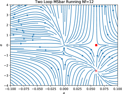
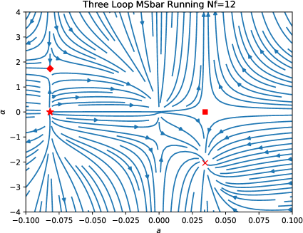
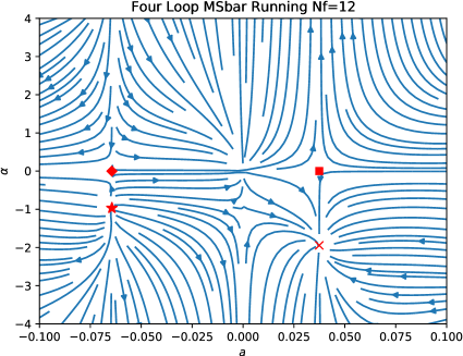
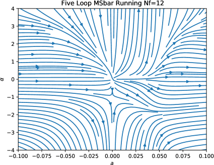
Figure 1: Flow plane for the $\overline{\mbox{MS}}$ scheme $SU(3)$ linear gauge at two, three, four and five loops when $N_{\!f}$ $=$ $12$

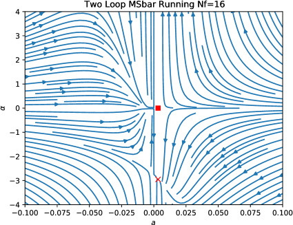
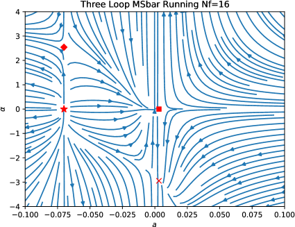
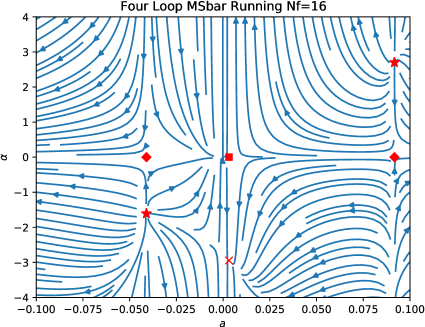
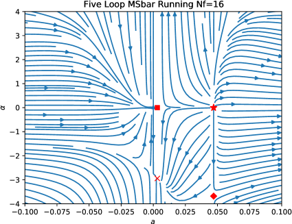
Figure 2: Flow plane for the $\overline{\mbox{MS}}$ scheme $SU(3)$ linear gauge at two, three, four and five loops when $N_{\!f}$ $=$ $16$

In order to visualize the renormalization group flow we have constructed flow plots in the coupling constant and gauge parameter plane. These are provided in Figures 1 and 2 for $SU(3)$ at two, three, four and five loops for $N_{\!f}$ $=$ $12$ and $16$ respectively in the case of the linear covariant gauge. The flow arrow is towards the infrared away from the Gaussian fixed point at the origin. Our notation is that a fixed point is indicated by various markers where their shapes indicate their stability property. In particular an infrared stable fixed point is indicated by $\times$, the Banks-Zaks critical point is denoted by $\blacksquare$ where the other saddle points are marked by $\blacklozenge$. The remaining shape, $\bigstar$, denotes an infrared unstable fixed point and therefore an ultraviolet stable one. Examining Figure 1 by way of example one sees the Banks-Zaks fixed point in line with its mirror partner at each loop order and $N_{\!f}$ value. By contrast infrared unstable fixed points are present at three and higher loops order but their location varies by a significant amount at successive orders and have no physical significance. The general locations of the Banks-Zaks and its stable mirror partner are clearly unaffected by the increasing loop order. The five loop plot of the flow for $N_{\!f}$ $=$ $12$ reflects the absence of the Banks-Zaks fixed point noted in [42].

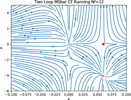
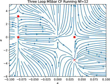
Figure 3: Flow plane for the $\overline{\mbox{MS}}$ scheme $SU(3)$ Curci-Ferrari gauge at two and three loops when $N_{\!f}$ $=$ $12$

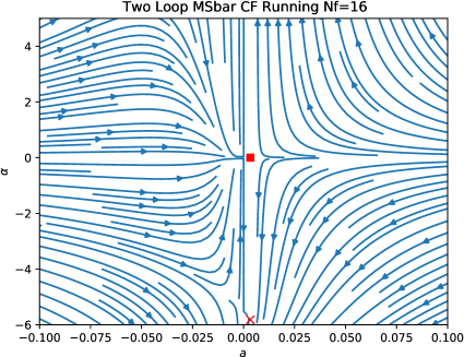
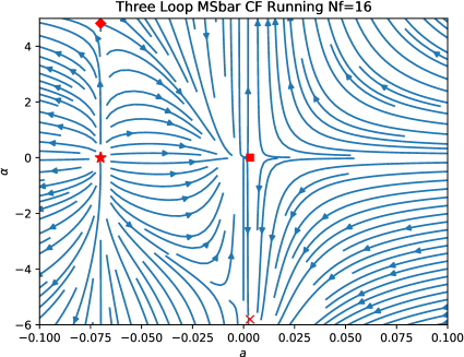
Figure 4: Flow plane for the $\overline{\mbox{MS}}$ scheme $SU(3)$ Curci-Ferrari gauge at two and three loops when $N_{\!f}$ $=$ $16$

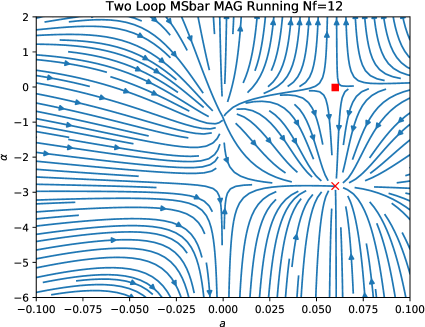
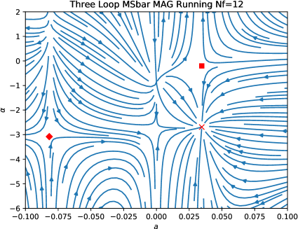
Figure 5: Flow plane for the $\overline{\mbox{MS}}$ scheme $SU(3)$ MAG at two and three loops when $N_{\!f}$ $=$ $12$

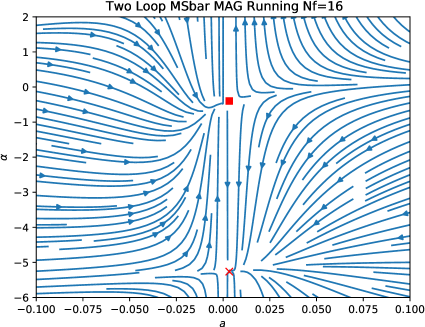
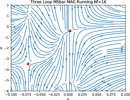
Figure 6: Flow plane for the $\overline{\mbox{MS}}$ scheme $SU(3)$ MAG at two and three loops when $N_{\!f}$ $=$ $16$

We have repeated the same analysis for the Curci-Ferrari gauge and MAG but only to three loop order as no renormalization group functions are available beyond that. While this may appear to limit what can be extracted from a fixed point analysis, it transpires that although a similar general picture emerges the details are necessarily different. The fixed point values at two and three loops together with their stability for the $\overline{\mbox{MS}}$ scheme are provided in Tables 6 and 7 for the Curci-Ferrari gauge with the parallel data for the MAG presented in Tables 8 and 9. Various flow plots for both gauges at two and three loops are provided in Figures 3 to 6. For both gauges we include three loop results for $N_{\!f}$ less than the perturbatively accepted value of $8$ for the lower boundary of the conformal window. This is to illustrate the changing nature of the Banks-Zaks fixed point in both gauges as it ceases being a saddle point and transforms into an infrared stable point when $N_{\!f}$ $\leq$ $7$. However for that range the analysis cannot be regarded as reliable as one is clearly beyond the region of perturbative validity. We need to qualify what we mean by a Banks-Zaks fixed point in the case of the MAG. In a linear gauge it corresponds to a non-trivial $\beta$-function zero in the $\overline{\mbox{MS}}$ scheme which is gauge parameter independent and so lies on the $\alpha$-axis in an $(a,\alpha)$ flow plot. Given the nature of the MAG gauge parameter anomalous dimension there is no fixed point when $\alpha$ $=$ $0$ but as is evident from Tables 8 and 9 there is a fixed point with a value of $\alpha$ close to zero. This is the one we refer to as the MAG Banks-Zaks fixed point. We have also checked that when the $N^{d}_{\!A}$ $\to$ $0$ limit is taken this fixed point smoothly tends to the Banks-Zaks fixed point of the Curci-Ferrari model. The flows for both gauges are given in Figures 3 and 4 for the Curci-Ferrari gauge and the corresponding ones for the MAG can be seen in Figures 5 and 6 where again we focus on $N_{\!f}$ $=$ $12$ and $16$. What is also apparent in the tables for the MAG is that an additional stable fixed point arises when $N_{\!f}$ $\leq$ $10$. Whether such extra solutions are an artefact of the loop order is not clear but they are present in an $N_{\!f}$ range where perturbative reliability could be questioned. One feature that differs from the linear covariant gauge is the value of the critical gauge parameter at the stable fixed point in both gauges. In the linear gauge the value was around $(-3)$ but in the two non-linear gauges the value appears to be in the neighbourhood of $(-5)$ for $N_{\!f}$ near the top end of the conformal window which has not been noted previously. Of course the parameters are not the same in each gauge and such parameters are not physically measureable. Their main application is in the determination of critical exponents which are renormalization group invariants and discussed later.

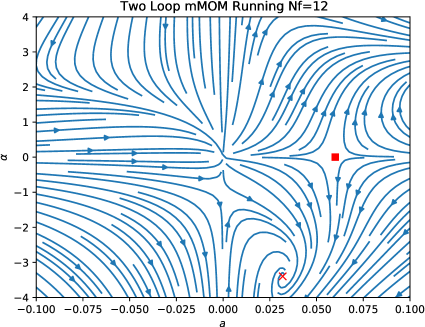
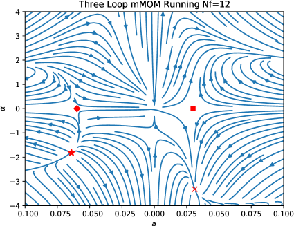
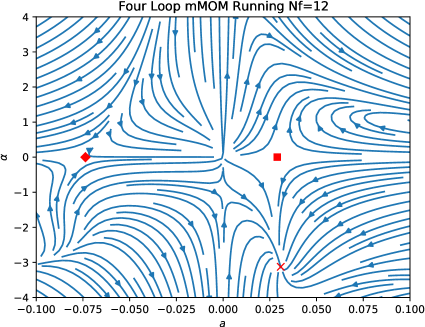
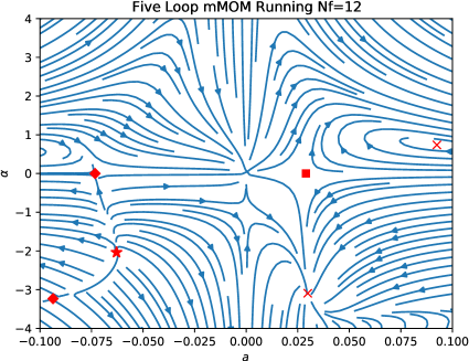
Figure 7: Flow plane for the mMOM scheme $SU(3)$ linear gauge at two, three, four and five loops when $N_{\!f}$ $=$ $12$

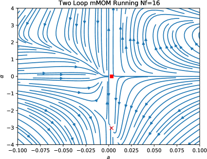
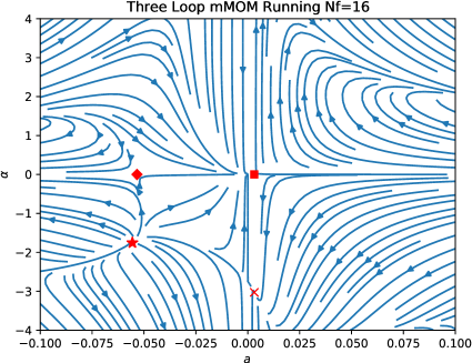
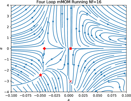
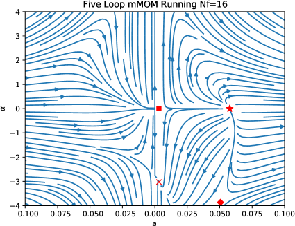
Figure 8: Flow planes for the mMOM scheme $SU(3)$ linear gauge at two, three, four and five loops when $N_{\!f}$ $=$ $16$

To this point the focus has been on the $\overline{\mbox{MS}}$ scheme for different gauges. It is instructive to analyse the fixed points in another scheme. As the renormalization group functions are available to five loops in the mMOM scheme [30, 31, 32, 33] for an arbitrary linear gauge parameter we have solved for the critical values of $a$ and $\alpha$ in that scheme. In this scheme the $\beta$-function depends on $\alpha$ in contrast to the $\overline{\mbox{MS}}$ scheme. The results for two, three, four and five loops are recorded in Tables 10, 11, 12 and 13 respectively. In general terms the tables reflect very similar properties to those observed in the $\overline{\mbox{MS}}$ scheme. The Banks-Zaks fixed point is evident across all loop orders and is a saddle point. The associated infrared stable fixed point is also a feature but with the caveat that it does not have the same critical coupling as the Banks-Zaks one. Instead its critical coupling value is very close to it. The critical gauge parameter value of the infrared stable points are all again in the neighbourhood of $\alpha$ $=$ $-$ $3$. For low loop order towards the lower end of the conformal window there is a larger deviation of this scenario. However at five loops there is a marked reduction in the discrepancy from $(-3)$ which is apparent at low $N_{\!f}$ values. This reinforces the $\overline{\mbox{MS}}$ observation that this gauge parameter choice may be a deeper property of the underlying theory. While the mMOM and the $\overline{\mbox{MS}}$ tables display a degree of similarity there are clearly several major differences. The first is that the eigenvalues of (2.9) are complex conjugates at several fixed points. The stability property is determined by the sign of the real part of the eigenvalues and the non-zero imaginary part indicates a spiral flow to or away from criticality. However as the loop order increases the spiral flow to the infrared stable fixed point appears to disappear. Perhaps the most significant aspect of the mMOM analysis is that there are real solutions for both $a$ and $\alpha$ for $N_{\!f}$ $\leq$ $12$ unlike the $\overline{\mbox{MS}}$ scheme. This therefore supports the five loop $\overline{\mbox{MS}}$ analysis of the Banks-Zaks critical point of [42] which required a Padé analysis to access fixed points for $N_{\!f}$ $\leq$ $12$. We have included all the real solutions to (2.8) partly for completeness but also for background when viewing the associated mMOM flow plots. These are given in Figures 7 and 8 for $N_{\!f}$ $=$ $12$ and $16$ respectively. Clearly some of the extra fixed points in the mMOM tables are beyond the region of perturbative validity. However their presence are responsible for the flow in the regions immediately outside the boundaries of the plots.

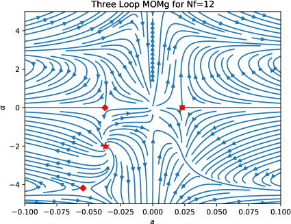
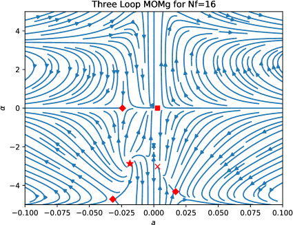
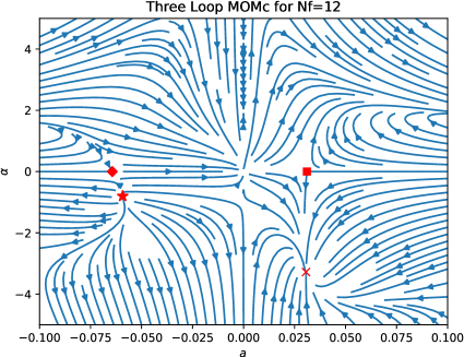
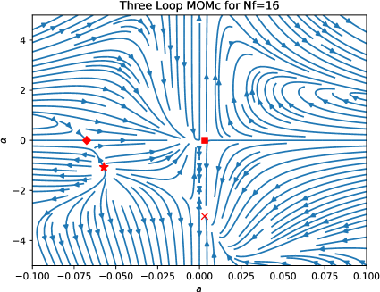
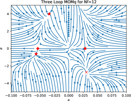
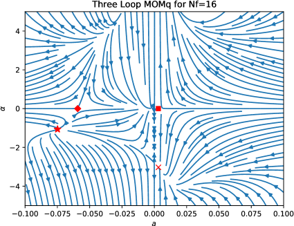
Figure 9: Flow planes for the three MOM schemes in $SU(3)$ at three loops for $N_{\!f}$ $=$ $12$ (left set) and $N_{\!f}$ $=$ $16$ (right set).

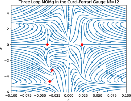
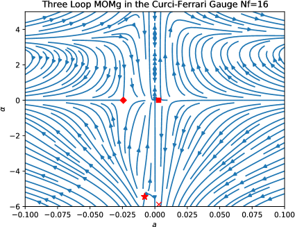
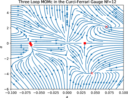
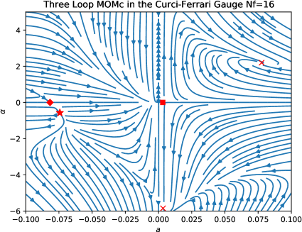
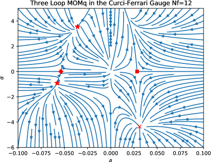
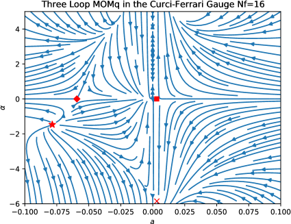
Figure 10: Flow planes for the three MOM schemes in $SU(3)$ Curci-Ferrari at three loops for $N_{\!f}$ $=$ $12$ (left set) and $N_{\!f}$ $=$ $16$ (right set).

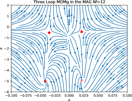
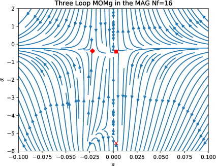
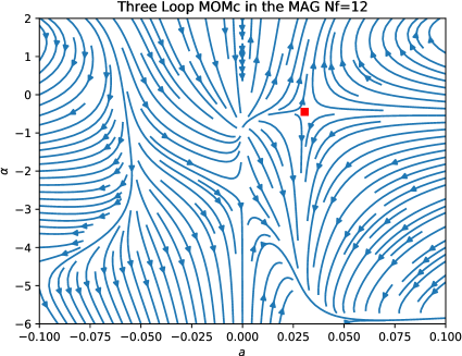
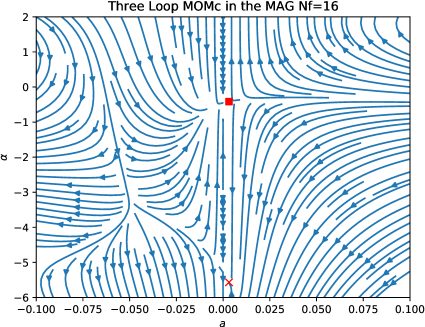
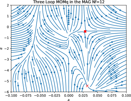
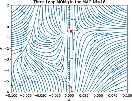
Figure 11: Flow planes for the three MOM schemes in $SU(3)$ MAG at three loops for $N_{\!f}$ $=$ $12$ (left set) and $N_{\!f}$ $=$ $16$ (right set).

We complete this section by recording the situation with the kinematic scheme fixed points in the three gauges of interest. Unlike the $\overline{\mbox{MS}}$ and mMOM schemes the full renormalization group functions for the MOM schemes of [35, 36] are only available at three loops for arbitrary gauge parameter. In order to compare the fixed point properties with other schemes we have provided the $N_{\!f}$ $=$ $12$ and $16$ three loop flow plots for the linear covariant and Curci-Ferrari gauges as well as the MAG in Figures 9, 10 and 11 respectively. In all three gauges and MOM schemes the Banks-Zaks and the infrared stable fixed points are clearly evident for $N_{\!f}$ $=$ $16$. For $N_{\!f}$ $=$ $12$ the situation is similar except in one or two schemes the infrared stable fixed point is not present in the flow plane. While the value of the critical gauge parameter of the infrared stable fixed point is consistently around the values of $(-3)$ for the linear gauge and $(-5)$ for the Curci-Ferrari gauge and MAG the associated critical coupling is actually large. While it is outside the range plotted it is also outside the domain of perturbative reliability. As an example Tables 14 and 15 record the fixed point data for the two and three loop MAG fixed points in the MOMc scheme. Given the improvement with convergence at $N_{\!f}$ $=$ $12$ that was apparent in the higher order $\overline{\mbox{MS}}$ and mMOM scheme fixed points we would expect that situation to improve if the full four loop renormalization group functions with $\alpha$ $\neq$ $0$ were available.

4 Critical exponents.

While the location of fixed points is important for understanding the renormalization group flow in QCD, the quantities of physical relevance are the critical exponents. Their values define the properties of the critical theory and are important for discerning the underlying conformal field theory at a fixed point. In our case values or estimates for the exponents are derived from the renormalization group functions of QCD by evaluating them at the various fixed points. In this section we will discuss the critical exponents derived from the anomalous dimensions of the gluon, ghost and quark fields as well as the quark mass dimension in the various gauges and schemes. The exponent derived from the quark mass anomalous dimension is gauge independent. So one aspect of our analysis will be to examine this in the various schemes and gauges. Moreover by comparing their values for a variety of schemes and gauges the issue of perturbative convergence can be examined. In addition the exponents $\omega_{1}$ and $\omega_{2}$ are derived from the underlying $\beta$-functions (2.10) and therefore should also be independent of the gauge fixing procedure. We qualify this outline of the analysis by recalling that data for the MOM kinematic schemes will be restricted to three loops unlike the $\overline{\mbox{MS}}$, mMOM and RI^′ schemes where five loop data are available. Previous exponent studies of the QCD critical points in various schemes was restricted to the Banks-Zaks fixed point in the $\overline{\mbox{MS}}$, RI^′ and mMOM schemes, [24, 25, 69, 70], and the kinematic schemes, [71]. Since we have examined the $(a,\alpha)$ flow plane in depth here our main focus will be on the exponents of the infrared stable fixed point. In the linear covariant gauge the value of the critical coupling for the Banks-Zaks and infrared stable fixed points are the same. Therefore there is a natural question as to whether the corresponding exponents are similar. If so this would reinforce the notion that the infrared stable fixed point is a mirror of the Banks-Zaks one.

First we concentrate on the four and five loop estimates for the $\overline{\mbox{MS}}$, mMOM and RI^′ schemes with values recorded in Tables 16 to 21. In these and other such tables the syntax is that BZ indicates Banks-Zaks and IRS denotes the infrared stable fixed point which is closest to the $\alpha$ axis on the flow plane. In addition type (IRS) in a table denotes another infrared stable fixed point that was identified in the corresponding earlier list of fixed points. Only Banks-Zaks and infrared stable fixed point exponents are recorded in the tables as exponents at saddle or infrared unstable fixed points are not of physical relevance. We recall that it is not always the case that values for exponents are available for each fixed point type across each scheme. Indeed this is not the case at five loops in the $\overline{\mbox{MS}}$ scheme as noted in [42] with the same situation for the RI^′ scheme since its $\beta$-function is formally the same as the $\overline{\mbox{MS}}$ one. The quantities $\gamma_{\phi}$ where $\phi$ $\in$ $\{A,c,\psi\}$ in the tables denote the critical exponents for the gluon, ghost and quark fields. The final column of each of our exponent tables will be the exponent $\rho_{m}$ which is related to the quark mass anomalous dimension and is given by

$$\rho_{m}~{}=~{}-~{}2\gamma_{\bar{\psi}\psi}(a_{\infty},\alpha_{\infty})~{}.$$ (4.1)

In focusing on the $\overline{\mbox{MS}}$, mMOM and RI^′ schemes in the first instance the four loop tables are provided for orientation with the main task of studying the effect of the next order correction. We note that exponent estimates for these and the MOM schemes had been recorded earlier in [72] for the Banks-Zaks critical point. That study together with [24] included results for $SU(2)$ and $SU(4)$ as well as for the quark in a variety of representations. For the $\rho_{m}$ exponent one obvious property that is evident here in the $\overline{\mbox{MS}}$ scheme at all loop orders is that the BZ and IRS values of $\rho_{m}$ are the same at each loop order. This follows simply from the fact that the anomalous dimension of the quark mass operator is gauge parameter independent in the $\overline{\mbox{MS}}$ scheme. Therefore the value of the critical gauge parameter is irrelevant for the exponent. In the mMOM and RI^′ schemes the quark mass operator does depend on the gauge parameter. So one would expect some deviation of the values for $\rho_{m}$ at the BZ and IRS fixed points. This is quite clearly the case at four loops for both schemes. Although at each fixed point for $N_{\!f}$ $=$ $15$ and $16$ $\rho_{m}$ is virtually identical which is the part of the conformal window where perturbative reliability is best. What is striking is that at five loops the value of $\rho_{m}$ at the BZ and IRS fixed points appear to show a marked convergence to a common value even down to $N_{\!f}$ $=$ $12$ for mMOM and $N_{\!f}$ $=$ $13$ for RI^′. Below that $N_{\!f}$ value for the RI^′ scheme there are no five loop solutions of (2.8). This strongly suggests that $\overline{\mbox{MS}}$ property of $\rho_{m}$ at the BZ and IRS fixed points will become a scheme independent property with more accuracy.

The convergence for the gluon, ghost and quark exponents is not as accurate except of course for the gluon at the IRS fixed point in the linear covariant gauge. This is because in that gauge the gluon anomalous and gauge parameter anomalous dimensions are equal and opposite and the vanishing of the latter is used to find the critical point values. For the BZ fixed point the gluon exponent is reasonably consistent down to $N_{\!f}$ $=$ $14$ for the three schemes at four and five loops. For $N_{\!f}$ $\leq$ $13$ there is a marked distinction between the value for RI^′ compared to the other two schemes. This can simply be put down to the lack of fixed points at five loops for $N_{\!f}$ $\leq$ $12$ in the $\overline{\mbox{MS}}$ and RI^′ schemes. The deviation is apparent at four loops. The picture for $\gamma_{c}$ is somewhat similar but with the value for the BZ fixed point is in better agreement across the three schemes even down to $N_{\!f}$ $=$ $12$ at five loops. By contrast the critical value of $\gamma_{\psi}$ at the IRS fixed point appears to be more consistent in the three schemes down to the $N_{\!f}$ $=$ $12$ demarcation. More importantly there is a clear improvement in convergence comparing the values of $\gamma_{\psi}$ at four loops with their five loop counterparts. This reinforces the earlier observation that the extra loop order is pointing to the emergence of a more accurate picture deeper into the conformal window. It is worth remarking at this point that a similar observation has been made recently in this respect but in a different context in [73]. There dimensionless ratios involving meson decay constants were studied in the conformal window using the perturbative expansion method about the Banks-Zaks fixed point introduced in [1]. Using a fourth order expansion $N_{\!f}$ $=$ $12$ was identified as a boundary where the perturbative approach was reliable, [73].

The situation with the kinematic schemes and non-linear gauges is not as clear cut. The values of exponents at three loops in the three MOM schemes and the gauges of interest are given in Tables 22 to 30. For the tables with MAG results the type (BZ) indicates the saddle point that would be in the neighbourhood of the Banks-Zaks fixed point of the other two gauges. In terms of relevance the gluon and ghost critical exponents can only be compared for convergence within each gauge and not in any other gauge. This is because these fields are not strictly the same object in different gauges. The only exponents that can be compared across gauges are $\rho_{m}$ and $\omega_{i}$. Examining $\rho_{m}$ for the MOM schemes shows up several patterns of consistency. First for $N_{\!f}$ close to the top of the conformal window the value of $\rho_{m}$ at both the Banks-Zaks and infrared stable fixed points are generally in very good agreement to three decimal places in the three gauges and MOM schemes. There is one exception though which is MOMg value at the infrared stable point in the Curci-Ferrari gauge. Similar exceptions to the general pattern for other exponents in the various gauges and schemes are apparent in the various tables. They can usually be attributed to accidental cancellations in evaluating the perturbative expansion. This actually lends weight to ensuring exponent estimates are derived in as many different ways as possible in order to the general trends. At lower values of $N_{\!f}$ in the conformal window the MOM scheme exponents are not as accurate as one would expect. For instance examining the $N_{\!f}$ $=$ $12$ case there is reasonable consistency at the Banks-Zaks point across the three gauges for each scheme. However there is a discrepancy across schemes within each gauge. For the infrared stable fixed point only the MOMq results have a degree of accuracy but the values for both fixed points undershoot the three loop $\overline{\mbox{MS}}$ values. We recall that at $N_{\!f}$ $=$ $12$ there is no infrared stable fixed point in the MOMg scheme. Clearly what is lacking for these lower values of $N_{\!f}$ are the higher order corrections in the perturbative series.

While the only four loop MOM scheme renormalization group functions that are available are in the Landau gauge, [39], we can try this information to probe whether the exponent convergence improves albeit at the Banks-Zaks fixed point. The results of this exercise are presented in Table 31 in the conformal window. What is evident from comparing the values of $\omega$ in the three schemes is that there is a degree of agreement for down to $N_{\!f}$ $=$ $14$ at which point the estimates in the MOMg scheme cease to be commensurate. In the MOMq case the values of $\omega$ are in reasonable agreement with those of MOMc down to $N_{\!f}$ $=$ $11$. What is interesting is that comparing the $\omega$ estimates for MOMc with the four loop mMOM ones there is remarkable agreement down to $N_{\!f}$ $=$ $9$. Although both schemes are based on the properties of the same vertex function the momentum configuration where the subtraction is carried out is different. One is for a non-exceptional momentum setup while the other is exceptional respectively. In this instance it would seem to reflect that there is an improvement in convergence. Comparing with the same region of the conformal window for the $\overline{\mbox{MS}}$ scheme is probably not a reliable exercise given that there was no five loop Banks-Zaks fixed point solution for low $N_{\!f}$. Regarding the MOMg scheme the drop off in the $\omega$ estimate as $N_{\!f}$ reduces might be indicative of a slow convergence or an indication that the Banks-Zaks fixed point might disappear at five loops. As such an eventuality arises in one scheme the same behaviour in another cannot be excluded.

The other exponents that should have a degree of consistency across schemes and gauges are those connected with corrections to scaling which are $\omega_{1}$ and $\omega_{2}$. First examining the $\overline{\mbox{MS}}$ values of $\omega_{i}$ in the linear covariant gauge in Tables 3, 4 and 5 several observations emerge that are also evident in other schemes and gauges. The obvious one is that one of the eigenvalues of (2.9) is the same for both the Banks-Zaks and infrared stable fixed point. Curiously the other stability eigenvalues are roughly equal in magnitude which is a feature of all $N_{\!f}$ values in the conformal window. Whether their equality will emerge with higher precision is an open question. Moreover the convergence from four to five loops is present down to $N_{\!f}$ $=$ $14$ but the loss of a solution for the conformal below $N_{\!f}$ $=$ $13$ is again reflected in the values for $\omega_{i}$ at this latter $N_{\!f}$ value. To gauge the structure at five loops better it is convenient to examine the $\omega_{i}$ for the mMOM scheme which are given in Tables 12 and 13 as the latter covers the conformal window more fully. Comparing the four loop values there is good agreement at the top of the conformal window down to $N_{\!f}$ $=$ $13$ but the positive exponent that is supposed to be the same at both the Banks-Zaks and infrared stable fixed points begin to differ at this $N_{\!f}$ value consistent with the appearance of the complex values for $\omega_{i}$ for $N_{\!f}$ $\leq$ $12$ and the switch of the stable infrared fixed point away from a critical gauge parameter value in the neighbourhood of $\alpha$ $=$ $-$ $3$. At five loops for both schemes the consistency for the top end of the window improves as expected from the increased perturbative accuracy. What is more striking though can be seen from the $N_{\!f}$ $=$ $13$ values of the four loop $\overline{\mbox{MS}}$ and five loop mMOM $\omega_{i}$ estimates. These are much more in keeping with each other indicating the importance of studying the properties in more than one scheme.

While these comments concern the linear covariant gauge in particular it is instructive to look at the situation in the two non-linear gauges. However for a fair comparison we will focus on the three loop values as nothing is available beyond beyond that order for the Curci-Ferrari gauge and MAG. First examining the values of $\omega_{i}$ in the linear covariant and Curci-Ferrari gauges given in Tables 2 and 7 there are several points to note. First while the $\omega_{2}$ values are the same for both fixed points in $9$ $\leq$ $N_{\!f}$ $\leq$ $16$ this reflects the $\alpha$ independence of the common $\beta$-function in both gauges in the $\overline{\mbox{MS}}$ scheme. What is more interesting is that the values $\omega_{1}$ are remarkably consistent for the same range of $N_{\!f}$ with a slight discrepancy in value at the lower end. What has to be remembered is that the critical gauge parameter for each $N_{\!f}$ value is not the same unlike the critical coupling. This lends weight to the observation that the infrared stable fixed point is a Banks-Zaks twin point. This pattern is less conclusive for the MOM schemes in the Curci-Ferrari gauge with only the MOMq data for $\omega_{i}$ producing comparable values with those in the $\overline{\mbox{MS}}$ scheme for $N_{\!f}$ down to $13$ flavours at three loops. In the MOMg scheme only in the $N_{\!f}$ $=$ $16$ case is there a stable infrared fixed point and then the $\omega_{i}$ values are not in keeping with the other schemes and gauges. This is again perhaps related to the absence of a similar critical point for lower values of $N_{\!f}$ in this scheme for the Curci-Ferrari gauge. The values for $\omega_{i}$ are not as accurate at the Banks-Zaks point either aside from $\omega_{2}$ down to $N_{\!f}$ $=$ $11$. For this fixed point in the MOMc scheme the situation at three loops is almost on a par with the MOMq results. However aside from $N_{\!f}$ $=$ $16$ the values of $\omega_{i}$ in the MOMc scheme are not reliable. In light of this one natural question concerns why the picture in the MOMq scheme is better than those in the MOMg and MOMc ones. Perhaps this can be explained by the position in the respective two loop cases. For MOMg there are no infrared stable fixed point solutions and only one appears at three loops unlike the linear covariant gauge. In the MOMc case at two loops there are infrared stable fixed points but aside from $N_{\!f}$ $=$ $16$ the $\omega_{i}$ are complex conjugates which become real at three loops. So it seems clear that for these two schemes the existence and properties of this infrared stable fixed point requires several more loop orders to become manifest on a comparable level to other schemes.

To complete our commentary on the situation with the corrections to scaling exponents we turn to the MAG results where the two and three loop $\overline{\mbox{MS}}$ results are given in Tables 8 and 9. Focusing for the moment on three loops it is clear that the $\omega_{2}$ value is in good agreement for a wide range of $N_{\!f}$ with the other two gauges. For the other exponent there is a wide disparity even for the fixed point close to the origin. This seems particularly peculiar given that the Curci-Ferrari gauge and MAG are intimately connected but the $\overline{\mbox{MS}}$ $\omega_{i}$ values are better aligned with those of the linear covariant gauge. This is perhaps indicative of a specific property of the MAG itself rather than a particular breakdown in the connection with the Curci-Ferrari gauge. In this respect we recall that the MAG treats the diagonal and off-diagonal gluons differently in the gauge fixing functional. The parameter $\alpha$ in this gauge relates to the non-linear gauge fixing for the off-diagonal gluons but the diagonal ones are fixed in the Landau gauge. In the same way that we explored the $(a,\alpha)$ plane for fixed points in the linear covariant and Curci-Ferrari gauge from the point of view of a critical point analysis of the renormalization group functions full gauge fixing a separate gauge parameter should be considered for the diagonal gluons. In other words the infrared stable fixed point associated with the gauge parameter in the neighbourhood of $\alpha$ $=$ $-$ $5$ may not be stable in the direction towards that extra gauge parameter. There may be an infrared stable fixed point in the $(a,\alpha,\bar{\alpha})$ hyperspace. If so then it would be the one for comparing the values of $\rho_{m}$ and two of the three $\omega_{i}$ exponents. Trying to explore this is beyond the scope of the present work. The reason for this is we would have to renormalize the QCD in a maximal abelian gauge fixing with one or more extra parameters. By this we mean that an interpolating gauge was constructed in [74] which involved six additional gauge parameters to ensure renormalizability. Taking separate limits of these parameters produces the usual linear covariant and maximal abelian gauges. Once these limits were verified at three loops one would then have to examine the fixed point structure to ascertain whether there was a stable infrared fixed point. If there were more than one such solution the absolute minimum should be the one that is the natural partner of the infrared stable fixed point of the other two gauges.

5 Padé analysis.

The absence of a Banks-Zaks fixed point at five loops in the $\overline{\mbox{MS}}$ scheme for the full range of the conformal window, [42], was unexpected. This was especially the case since perturbative estimates of the $\rho_{m}$ exponent are of importance to compare with lattice methods. Consequently an additional tool was employed to explore the lower reaches of the conformal window in this scheme which was Padé approximants, [42]. The approach was to establish a more accurate fixed point and thence a better estimate of $\rho_{m}$. Given that our five loop mMOM analysis has revealed that the absence of the $\overline{\mbox{MS}}$ five loop Banks-Zaks fixed point can be attributed to a scheme artefact it is a worthwhile exercise to repeat the Padé analysis of [42] for the mMOM scheme but also for the RI^′ one. By doing so we will be able to see if a consensus emerges for exponent values at the lower end of the conformal window below $N_{\!f}$ $\leq$ $12$. Moreover we will not restrict the analysis to the Banks-Zaks case but include its twin partner. To facilitate such a study therefore requires incorporating the gauge parameter into the rational polynomials of the Padé approximants.

By way of establishing our approach we focus first on the $\overline{\mbox{MS}}$ scheme with the aim of reproducing the data of [42] for the Banks-Zaks case which will also play the role of a check on the setup as it will include $\alpha$ dependence. This will be of importance for the mirror fixed point since ultimately exponent estimates should be independent of the gauge. As before searching for stationary running means searching for solutions $(a_{\infty},\alpha_{\infty})$ to $\beta(a_{\infty},\alpha_{\infty})$ $=$ $0$ and $\alpha_{\infty}\gamma_{\alpha}(a_{\infty},\alpha_{\infty})$ $=$ $0$. However both $\beta(a,\alpha)$ and $\gamma_{\alpha}(a,\alpha)$ will be supplied by Padé approximants such that

$$\beta^{[p,q]}(a,\alpha) = \beta_{0}a^{2}\ \frac{\left[1+\sum_{j=1}^{p}u^{[p,q]}_{j}(\alpha)a^{j}\right]}{\left[1+\sum_{k=1}^{q}v^{[p,q]}_{k}(\alpha)a^{k}\right]}$$

$$\gamma_{\alpha}^{[p,q]}(a,\alpha) = \gamma_{1}a\frac{\left[1+\sum_{j=1}^{p}w^{[p,q]}_{j}(\alpha)a^{j}\right]}{\left[1+\sum_{k=1}^{q}x^{[p,q]}_{k}(\alpha)a^{k}\right]}$$ (5.1)

where

$$\beta_{0}~{}=~{}-~{}\frac{1}{3}[11C_{A}-4T_{F}N_{\!f}]~{}~{}~{},~{}~{}~{}\gamma_{1}~{}=~{}\frac{1}{6}[8T_{F}N_{\!f}-13C_{A}+3\alpha C_{A}]$$ (5.2)

and only $a$ acts as the expansion parameter in the approximant with $\alpha$ entering in the coefficients. While we could have approximated $\beta(a,\alpha)$ and $\alpha\gamma_{\alpha}(a,\alpha)$ with different $[p,q]$ approximants, since any approximation will be correct to the order in perturbation theory we consider here, for simplicity we have used the same $[p,q]$ structure for both functions. Although we use the same method as Section $3$ to search for fixed point solutions we need to ensure they are in the region of validity of the approximation. By this we mean the approximant to both renormalization group functions has no poles or denominator zeros that are closer to the axis than the critical point when the gauge parameter is fixed to $\alpha_{\infty}$. The fixed points will be classified into three categories. The first class is the valid fixed points which are those for which no zero of the denominator has a smaller absolute coupling constant value than the fixed point. The second class is termed the zero pole (zp) fixed points which are those where there exist zeros in the denominator closer to the origin than the fixed point but these are also zeros of the numerator. Thus these zero pole zero numerator pair will cancel each other. The final group are critical points with a pole closer to $a$ $=$ $0$ but these will be discarded from further analysis. With regard to using the critical point data for the first two classes the last step will be to determine the quark mass anomalous dimension. We do this by evaluating the regular polynomial perturbative series for the renormalization group function at the fixed point.

The results of our Padé analysis for the $\overline{\mbox{MS}}$ scheme are recorded in Table 32. Since the values of the coupling constant and quark mass exponent have already appeared in [42] it is satisfying to note that we find full agreement allowing for the difference in convention for the coupling constant. Given that reassuring check we now restrict the discussion to the sector with non-zero gauge parameter values. Since the $\beta$-function and mass anomalous dimension are gauge parameter independent in the $\overline{\mbox{MS}}$ scheme we again see that their values are consistent across multiple gauge parameter values. As all approximations presented are accurate to an order in perturbation theory within their region of validity, if we can identify the Banks-Zaks’ twin then we can use the values from different approximations to provide a range for the location of the fixed point. We note the fixed point we label as the Banks-Zaks twin is chosen on the basis of consistency across schemes, loop order, anomalous dimensions and $N_{\!f}$ but still its identification is not absolutely defined. As one would expect of something whose value is accurate to the truncation order under consideration we see that the critical gauge parameter values are more congruous with like values in the other approximations at high $N_{\!f}$ where the corresponding $a_{\infty}$ is lower than at smaller $N_{\!f}$. For example, at $N_{\!f}$ $=$ $16$ the difference provided by these values is $5\times 10^{-6}$, whereas at $N_{\!f}$ $=$ $13$ this difference is $0.03$. While there were more fixed points outside of the region of validity it is of interest to note that in this case the fixed points that were retained for the different Padé approximants are, in the case of $[2,2]$ and $[1,3]$, only the Banks-Zaks fixed point and its partner. For $N_{\!f}$ $=$ $12$ we can compare the non-zero gauge parameter for the $[3,1]$ approximant with those of the other approximants in order to ask whether the zp fixed points provide an accurate representation of the fixed point. In this case we see the difference between the $[3,1]$ fixed point and the $[1,3]$ fixed point is roughly ten times the difference between $[2,2]$ and $[1,3]$ in both the coupling constant and the gauge parameter. While this is not necessarily promising, we point out that the quark mass exponent values are not considerably more consistent between the valid fixed points than between the zp and valid fixed points. We will not draw any firm conclusions about this before examining other schemes.

With regard to this the critical coupling constants are the same in the $\overline{\mbox{MS}}$ and RI^′ scheme because their $\beta$-functions are formally equivalent. However the two schemes are unique and the gauge parameter running of both is different. This therefore allows for a simple point of comparison in relation to their Padé approximations. Table 33 gives the RI^′ scheme results that is the parallel to Table 32 and is accurate to the five loop level. First we note that the location of the secondary $\alpha$ $=$ $0$ fixed point changes drastically between $[4,0]$ and $[3,1]$ approximants even at $N_{\!f}$ $=$ $16$. This suggests this value is not perturbatively reliable. By contrast the Banks-Zaks fixed point value itself is stable for the entire conformal window when compared between different Padé approximants. This is as expected since the critical coupling constant values are the same as in the $\overline{\mbox{MS}}$ scheme as they ought to be given the way the two scheme $\beta$-functions are related. While the mass anomalous dimension is not gauge parameter independent in the RI^′ scheme, we will identify the Banks-Zaks twin as the fixed point whose $\rho_{m}$ and coupling constant best matches the Banks-Zaks values. At $N_{\!f}$ $=$ $16$ the Banks-Zaks twin is approximately in the same place in all Padé approximants with a range of $0.000030$ between the maximum and minimum values. It is less clear what would be referred to as the Banks-Zaks twin at lower $N_{\!f}$ values since the truncation errors affect both the mass exponent and the gauge parameter position. At $N_{\!f}$ $=$ $14$ this value is at $\alpha$ $\approx$ $-$ $4$ with a range of $0.2$ but at $N_{\!f}$ $=$ $13$ this range is $2$. Below this we cannot identify any with this on more than one approximant. At the upper end of the conformal window the value of $\rho_{m}$ is consistent for the different Banks-Zaks pairs across the different approximations. This decreases as we move towards the lower end. At $N_{\!f}$ $=$ $13$ the values are compatible with values of approximately $0.19$ and a secondary value of $0.3$ appears for some of the other fixed points. As only the $[3,1]$ approximant has a positive $\rho_{m}$ as $N_{\!f}$ is reduced, further comparison is difficult beyond this point. However considering the four loop approximation we do see agreement between fixed point values at $N_{\!f}$ $=$ $12$ but not really lower $N_{\!f}$.

We close this section by extending this analysis to schemes with a gauge parameter dependent $\beta$-function which means the mMOM scheme as it is the only one available at five loops. The results are given in Table 34. Examining $N_{\!f}$ $=$ $16$ we again see good agreement between the two critical point parameters and the quark mass exponent calculated at the fixed points for the different Padé approximants. The case $N_{\!f}$ $=$ $14$ provides us with the first zero pole pair fixed point which has a close analogue in the set of fixed points in the canonical perturbative expansion. However at $N_{\!f}$ $=$ $10$ this is no longer the case with a range of values from $0.056$ for the $[3,1]$ zp case to $0.024$ for the $[1,3]$ fixed point with the $[2,2]$ approximant best matching the fixed point from the regular expansion. At $N_{\!f}$ $=$ $11$ the critical coupling constant value for the $[3,1]$ zp approximant is congruous with that of the Banks-Zaks one as well as showing agreement with the mass exponent suggesting that the zp fixed points should be taken into consideration. Examining the range of gauge parameter values for the Banks-Zaks twin we find it is $3\times 10^{-6}$ when $N_{\!f}$ $=$ $16$, $0.004$ at $N_{\!f}$ $=$ $13$ but $2$ at $N_{\!f}$ $=$ $10$ if we include the $\alpha$ $=$ $-$ $1.6$ fixed point for the $[1,3]$ approximant. In this case the critical coupling constant has a difference of $0.01$ which is at the same order as the coupling constant itself. For the quark mass exponent of the Banks-Zaks fixed points we see again a decreasing degree of consistency as $N_{\!f}$ decreases. For $N_{\!f}$ $=$ $14$ where we find a zp there is still a good compatibility between this value and those calculated for the Banks-Zaks fixed point of the other approximants. Even at $N_{\!f}$ $=$ $12$ we see good agreement with a range of values from $0.306$ to $0.284$.

6 Discussion.

We have provided a comprehensive analysis of the fixed point structure of the renormalization group functions in QCD where the gauge parameter is treated as an additional coupling constant. While there have been earlier studies in this respect, [41], which revealed interesting structure given the progress in determining the renormalization group functions to much higher order in recent years it was important to revisit that work. This was not just in the context of one scheme and gauge. Instead our analysis not only included the canonical linear covariant gauge fixing as well as the $\overline{\mbox{MS}}$ and MOM schemes of [35, 36] we incorporated the RI^′ and mMOM schemes in addition to two nonlinear covariant gauges. Although five loop results are not yet available for the latter two gauges it was important to study the extent to which critical exponent estimates of observables were not only scheme independent but also independent of the choice of gauge. This is because when solving for the fixed points numerically, as with any perturbative truncation, there will always be a degree of tolerance in final estimates. Within the conformal window at the centre of our investigation one of the main observations was that in the regime where the perturbative approximation is reliable good agreement with exponent estimates across schemes and gauges emerged. Indeed where five loop results were available it was clear that these higher orders increased the range of perturbative applicability. In addition at five loops the absence of a solution for the Banks-Zaks fixed point in the $\overline{\mbox{MS}}$ scheme for $N_{\!f}$ $\leq$ $12$ was shown to be a scheme artefact. Instead solving for the zeros of the $\beta$-functions in the mMOM scheme produced solutions at and below $N_{\!f}$ $=$ $12$ at five loops. With data from these two schemes as well as the RI^′ one Padé approximants were used to study if convergence could be improved away from the top end of the conformal window.

One observation of [41] was the existence of a fixed point in the interior of the $(a,\alpha)$ plane away from either axis in addition to the Gaussian and Banks-Zaks one. As its critical coupling in the linear covariant gauge was the same as the latter fixed point we referred to this as its mirror or twin fixed point. Moreover we verified that it was infrared stable unlike the Banks-Zaks one which is a saddle point on the $(a,\alpha)$ plane. To answer the obvious question as to whether this was an artefact of the linear covariant gauge we searched for a similar infrared stable fixed point in the two non-linear covariant gauges. Intriguingly such a similar critical point is present in both cases. While this is qualified by noting that the critical gauge parameter value differ in each of the three gauges since this is not an observable what did emerge was the consistency of the estimate for the critical exponent $\rho_{m}$ in the region of perturbative reliability at this infrared stable point. Moreover in the MAG the Banks-Zaks fixed point is absent in the conventional sense since there is no point on the coupling constant axis although there is a saddle point in its neighbourhood. Given that the existence of such a stable infrared critical point in QCD appears to be independent of the covariant gauge fixing procedure it reinforces the observation of [41] that retaining the gauge parameter in studies might assist infrared analyses of colour confinement. This would be an interesting topic to pursue but would clearly require a non-perturbative approach. Finally we remark that we have completely focused on the $SU(3)$ colour group with quarks in the fundamental representation. There is no a priori reason why one should restrict gauge theory fixed point analyses to this particular Lie group or matter representation. Rather it might be of interest to embed the $SU(3)$ analysis in the Standard Model as well as other gauge theories that seek to explore beyond that fundamental theory. Indeed in this context it is worth noting that the choice of $\alpha$ $=$ $-$ $3$ for the linear covariant gauge fixing in the electroweak sector was singled out as a special case in [75]. In particular at this value the $Z$ boson is renormalized multiplicatively.

Acknowledgements. This work was carried out with the support of the STFC Consolidated Grant ST/T000988/1 (JAG), an EPSRC Studentship EP/R513271/1 (RHM) and an STFC Studentship ST/M503629/1 (RMS). For the purpose of open access, the authors have applied a Creative Commons Attribution (CC-BY) licence to any Author Accepted Manuscript version arising. The data representing the full fixed point and critical exponent analysis of the work presented here are accessible in electronic form from the arXiv ancillary directory associated with the article.

$N_{\!f}$	$a_{\infty}$	$\alpha_{\infty}$	$\omega_{1}$	$\omega_{2}$	Infrared Stability
9	$0.416667$	$0.000000$	$-4.153646$	$2.083333$	Saddle
	$0.416667$	$-2.146730$	$2.353470$	$2.083333$	Stable
	$0.416667$	$-4.953270$	$-5.430293$	$2.083333$	Saddle
10	$0.175676$	$0.000000$	$-1.118449$	$0.761261$	Saddle
	$0.175676$	$-2.303972$	$0.749845$	$0.761261$	Stable
	$0.175676$	$-6.990900$	$-2.275239$	$0.761261$	Saddle
11	$0.098214$	$0.000000$	$-0.520338$	$0.360119$	Saddle
	$0.098214$	$-2.432707$	$0.391895$	$0.360119$	Stable
	$0.098214$	$-9.855172$	$-1.587611$	$0.360119$	Saddle
12	$0.060000$	$0.000000$	$-0.290250$	$0.180000$	Saddle
	$0.060000$	$-2.548046$	$0.237660$	$0.180000$	Stable
	$0.060000$	$-14.063065$	$-1.311685$	$0.180000$	Saddle
13	$0.037234$	$0.000000$	$-0.171886$	$0.086879$	Saddle
	$0.037234$	$-2.655694$	$0.149886$	$0.086879$	Stable
	$0.037234$	$-20.749068$	$-1.171065$	$0.086879$	Saddle
14	$0.022124$	$0.000000$	$-0.099863$	$0.036873$	Saddle
	$0.022124$	$-2.758253$	$0.091485$	$0.036873$	Stable
	$0.022124$	$-32.875081$	$-1.090390$	$0.036873$	Saddle
15	$0.011364$	$0.000000$	$-0.050894$	$0.011364$	Saddle
	$0.011364$	$-2.857085$	$0.048523$	$0.011364$	Stable
	$0.011364$	$-61.309582$	$-1.041235$	$0.011364$	Saddle
16	$0.003311$	$0.000000$	$-0.014853$	$0.001104$	Saddle
	$0.003311$	$-2.952985$	$0.014638$	$0.001104$	Stable
	$0.003311$	$-203.880349$	$-1.010609$	$0.001104$	Saddle

Table 1: Two loop $\overline{\mbox{MS}}$ scheme $SU(3)$ fixed points in the linear covariant gauge in the conformal window.

$N_{\!f}$	$a_{\infty}$	$\alpha_{\infty}$	$\omega_{1}$	$\omega_{2}$	Infrared Stability
9	$0.081803$	$0.000000$	$-0.193341$	$0.737728$	Saddle
	$0.081803$	$-0.858773$	$0.172635$	$0.737728$	Stable
10	$0.060824$	$0.000000$	$-0.175883$	$0.435887$	Saddle
	$0.060824$	$-1.298293$	$0.154800$	$0.435887$	Stable
11	$0.046039$	$0.000000$	$-0.151892$	$0.258488$	Saddle
	$0.046039$	$-1.692825$	$0.134329$	$0.258488$	Stable
12	$0.034607$	$0.000000$	$-0.125974$	$0.147759$	Saddle
	$0.034607$	$-2.039860$	$0.113066$	$0.147759$	Stable
13	$0.025191$	$0.000000$	$-0.099007$	$0.077790$	Saddle
	$0.025191$	$-2.339613$	$0.090641$	$0.077790$	Stable
14	$0.017070$	$0.000000$	$-0.071194$	$0.034949$	Saddle
	$0.017070$	$-2.591922$	$0.066678$	$0.034949$	Stable
15	$0.009818$	$0.000000$	$-0.042753$	$0.011153$	Saddle
	$0.009818$	$-2.795125$	$0.041052$	$0.011153$	Stable
16	$0.003162$	$0.000000$	$-0.014138$	$0.001102$	Saddle
	$0.003162$	$-2.945839$	$0.013943$	$0.001102$	Stable

Table 2: Three loop $\overline{\mbox{MS}}$ scheme $SU(3)$ fixed points in the linear covariant gauge in the conformal window.

$N_{\!f}$	$a_{\infty}$	$\alpha_{\infty}$	$\omega_{1}$	$\omega_{2}$	Infrared Stability
9	$0.085291$	$0.000000$	$0.017807$	$0.732193$	Stable
	$0.085291$	$0.078057$	$-0.018214$	$0.732193$	Saddle
	$0.085291$	$-5.882389$	$-1.983191$	$0.732193$	Saddle
	$0.962002$	$0.000000$	$-542.394739$	$3638.528050$	Saddle
	$0.962002$	$2.372214$	$-12107.306162$	$-542.394739$	Unstable
	$0.962002$	$-2.710372$	$-4877.065906$	$-542.394739$	Unstable
10	$0.064860$	$0.000000$	$-0.096514$	$0.426703$	Saddle
	$0.064860$	$-0.758788$	$0.084116$	$0.426703$	Stable
	$0.064860$	$-7.285851$	$-1.593756$	$0.426703$	Saddle
	$0.446940$	$0.000000$	$-72.410221$	$216.607652$	Saddle
	$0.446940$	$2.631336$	$-770.095520$	$-72.410221$	Unstable
	$0.446940$	$-2.802990$	$-276.712319$	$-72.410221$	Unstable
11	$0.049832$	$0.000000$	$-0.125835$	$0.249017$	Saddle
	$0.049832$	$-1.444524$	$0.107670$	$0.249017$	Stable
	$0.049832$	$-9.164022$	$-1.495291$	$0.249017$	Saddle
	$0.262159$	$0.000000$	$-18.805627$	$32.056161$	Saddle
	$0.262159$	$2.797166$	$-114.552315$	$-18.805627$	Unstable
	$0.262159$	$-3.009747$	$-40.855724$	$-18.805627$	Unstable
12	$0.037434$	$0.000000$	$-0.121873$	$0.141164$	Saddle
	$0.037434$	$-1.945284$	$0.106950$	$0.141164$	Stable
	$0.037434$	$-11.872619$	$-1.477787$	$0.141164$	Saddle
	$0.182641$	$0.000000$	$-8.151111$	$9.044557$	Saddle
	$0.182641$	$2.874023$	$-31.268962$	$-8.151111$	Unstable
	$0.182641$	$-3.270103$	$-11.852903$	$-8.151111$	Unstable

Table 3: Four loop $\overline{\mbox{MS}}$ scheme $SU(3)$ fixed points in the linear covariant gauge for $9$ $\leq$ $N_{\!f}$ $\leq$ $12$.

$N_{\!f}$	$a_{\infty}$	$\alpha_{\infty}$	$\omega_{1}$	$\omega_{2}$	Infrared Stability
13	$0.026853$	$0.000000$	$-0.101310$	$0.074565$	Saddle
	$0.026853$	$-2.312632$	$0.091708$	$0.074565$	Stable
	$0.026853$	$-16.124358$	$-1.476144$	$0.074565$	Saddle
	$0.141687$	$0.000000$	$-4.907150$	$3.754144$	Saddle
	$0.141687$	$2.881045$	$-12.298078$	$-4.907150$	Unstable
	$0.141687$	$-3.553712$	$-5.175980$	$-4.907150$	Unstable
14	$0.017793$	$0.000000$	$-0.073373$	$0.033906$	Saddle
	$0.017793$	$-2.588296$	$0.068423$	$0.033906$	Stable
	$0.017793$	$-23.713794$	$-1.471549$	$0.033906$	Saddle
	$0.117756$	$0.000000$	$-3.633611$	$1.980404$	Saddle
	$0.117756$	$2.842775$	$-6.094849$	$-3.633611$	Unstable
	$0.117756$	$-3.843479$	$-2.923578$	$-3.633611$	Unstable
15	$0.010001$	$0.000000$	$-0.043478$	$0.010988$	Saddle
	$0.010001$	$-2.795819$	$0.041706$	$0.010988$	Stable
	$0.010001$	$-41.152460$	$-1.462900$	$0.010988$	Saddle
	$0.102368$	$0.000000$	$-3.051413$	$1.218110$	Saddle
	$0.102368$	$2.778768$	$-3.516462$	$-3.051413$	Unstable
	$0.102368$	$-4.129750$	$-1.950938$	$-3.051413$	Unstable
16	$0.003170$	$0.000000$	$-0.014174$	$0.001099$	Saddle
	$0.003170$	$-2.945935$	$0.013978$	$0.001099$	Stable
	$0.003170$	$-126.835296$	$-1.453369$	$0.001099$	Saddle
	$0.091700$	$0.000000$	$-2.761435$	$0.828759$	Saddle
	$0.091700$	$2.700828$	$-2.247803$	$-2.761435$	Unstable
	$0.091700$	$-4.407403$	$-1.453956$	$-2.761435$	Unstable

Table 4: Four loop $\overline{\mbox{MS}}$ scheme $SU(3)$ fixed points in the linear covariant gauge for $13$ $\leq$ $N_{\!f}$ $\leq$ $16$.

$N_{\!f}$	$a_{\infty}$	$\alpha_{\infty}$	$\omega_{1}$	$\omega_{2}$	Infrared Stability
13	$0.032315$	$0.000000$	$-0.122684$	$0.036682$	Saddle
	$0.032315$	$-2.386609$	$0.109561$	$0.036682$	Stable
	$0.041343$	$0.000000$	$-0.151397$	$-0.072312$	Unstable
	$0.041343$	$-2.470802$	$0.131351$	$-0.072312$	Saddle
14	$0.018526$	$0.000000$	$-0.076782$	$0.031152$	Saddle
	$0.018526$	$-2.603426$	$0.071510$	$0.031152$	Stable
	$0.046357$	$0.000000$	$-0.365291$	$-0.176646$	Unstable
	$0.046357$	$-2.932818$	$0.152600$	$-0.365291$	Saddle
15	$0.010078$	$0.000000$	$-0.043850$	$0.010828$	Saddle
	$0.010078$	$-2.797897$	$0.042058$	$0.010828$	Stable
	$0.047107$	$0.000000$	$-0.587861$	$-0.190657$	Unstable
	$0.047107$	$-3.326390$	$0.168639$	$-0.587861$	Saddle
16	$0.003171$	$0.000000$	$-0.014178$	$0.001098$	Saddle
	$0.003171$	$-2.945965$	$0.013982$	$0.001098$	Stable
	$0.046999$	$0.000000$	$-0.780464$	$-0.202969$	Unstable
	$0.046999$	$-3.682521$	$0.185665$	$-0.780464$	Saddle

Table 5: Five loop $\overline{\mbox{MS}}$ scheme $SU(3)$ fixed points in the linear covariant gauge for $13$ $\leq$ $N_{\!f}$ $\leq$ $16$.

$N_{\!f}$	$a_{\infty}$	$\alpha_{\infty}$	$\omega_{1}$	$\omega_{2}$	Infrared Stability
9	$0.416667$	$0.000000$	$-4.153646$	$2.083333$	Saddle
	$0.416667$	$-2.387888$	$3.596809$	$2.083333$	Stable
	$0.416667$	$-17.812112$	$-26.829882$	$2.083333$	Saddle
10	$0.175676$	$0.000000$	$-1.118449$	$0.761261$	Saddle
	$0.175676$	$-2.981627$	$0.964118$	$0.761261$	Stable
	$0.175676$	$-21.608116$	$-6.987048$	$0.761261$	Saddle
11	$0.098214$	$0.000000$	$-0.520338$	$0.360119$	Saddle
	$0.098214$	$-3.548192$	$0.452028$	$0.360119$	Stable
	$0.098214$	$-27.027566$	$-3.443224$	$0.360119$	Saddle
12	$0.060000$	$0.000000$	$-0.290250$	$0.180000$	Saddle
	$0.060000$	$-4.078489$	$0.256566$	$0.180000$	Stable
	$0.060000$	$-35.143733$	$-2.210791$	$0.180000$	Saddle
13	$0.037234$	$0.000000$	$-0.171886$	$0.086879$	Saddle
	$0.037234$	$-4.569040$	$0.155606$	$0.086879$	Stable
	$0.037234$	$-48.240484$	$-1.642904$	$0.086879$	Saddle
14	$0.022124$	$0.000000$	$-0.099863$	$0.036873$	Saddle
	$0.022124$	$-5.020489$	$0.092924$	$0.036873$	Stable
	$0.022124$	$-72.246178$	$-1.337198$	$0.036873$	Saddle
15	$0.011364$	$0.000000$	$-0.050894$	$0.011364$	Saddle
	$0.011364$	$-5.435844$	$0.048748$	$0.011364$	Stable
	$0.011364$	$-128.897489$	$-1.155936$	$0.011364$	Saddle
16	$0.003311$	$0.000000$	$-0.014853$	$0.001104$	Saddle
	$0.003311$	$-5.819105$	$0.014644$	$0.001104$	Stable
	$0.003311$	$-413.847562$	$-1.041453$	$0.001104$	Saddle

Table 6: Two loop $\overline{\mbox{MS}}$ scheme $SU(3)$ Curci-Ferrari gauge fixed points for $9$ $\leq$ $N_{\!f}$ $\leq$ $16$.

$N_{\!f}$	$a_{\infty}$	$\alpha_{\infty}$	$\omega_{1}$	$\omega_{2}$	Infrared Stability
6	$1.012686$	$0.000000$	$40.841486$	$92.653913$	Stable
	$1.012686$	$0.773985$	$-101.745391$	$40.841486$	Saddle
7	$0.195518$	$0.000000$	$0.161289$	$2.986261$	Stable
	$0.195518$	$0.134812$	$-0.163479$	$2.986261$	Saddle
8	$0.116505$	$0.000000$	$-0.176683$	$1.329441$	Saddle
	$0.116505$	$-0.525277$	$0.169160$	$1.329441$	Stable
9	$0.081803$	$0.000000$	$-0.193341$	$0.737728$	Saddle
	$0.081803$	$-1.239118$	$0.177887$	$0.737728$	Stable
10	$0.060824$	$0.000000$	$-0.175883$	$0.435887$	Saddle
	$0.060824$	$-1.988405$	$0.158258$	$0.435887$	Stable
11	$0.046039$	$0.000000$	$-0.151892$	$0.258488$	Saddle
	$0.046039$	$-2.744498$	$0.135852$	$0.258488$	Stable
12	$0.034607$	$0.000000$	$-0.125974$	$0.147759$	Saddle
	$0.034607$	$-3.479125$	$0.113468$	$0.147759$	Stable
13	$0.025191$	$0.000000$	$-0.099007$	$0.077790$	Saddle
	$0.025191$	$-4.169158$	$0.090635$	$0.077790$	Stable
14	$0.017070$	$0.000000$	$-0.071194$	$0.034949$	Saddle
	$0.017070$	$-4.796907$	$0.066620$	$0.034949$	Stable
15	$0.009818$	$0.000000$	$-0.042753$	$0.011153$	Saddle
	$0.009818$	$-5.347954$	$0.041032$	$0.011153$	Stable
16	$0.003162$	$0.000000$	$-0.014138$	$0.001102$	Saddle
	$0.003162$	$-5.808458$	$0.013942$	$0.001102$	Stable

Table 7: Three loop $\overline{\mbox{MS}}$ scheme $SU(3)$ Curci-Ferrari gauge fixed points for $6$ $\leq$ $N_{\!f}$ $\leq$ $16$.

$N_{\!f}$	$a_{\infty}$	$\alpha_{\infty}$	$\omega_{1}$	$\omega_{2}$	Infrared Stability
9	$0.416667$	$0.373983$	$-14.338702$	$2.083333$	Saddle
	$0.416667$	$-1.775685$	$12.032176$	$2.083333$	Stable
	$0.416667$	$-12.989602$	$-74.798981$	$2.083333$	Saddle
10	$0.175676$	$0.246040$	$-2.897017$	$0.761261$	Saddle
	$0.175676$	$-2.041475$	$2.432727$	$0.761261$	Stable
	$0.175676$	$-14.027308$	$-15.179420$	$0.761261$	Saddle
11	$0.098214$	$0.113996$	$-1.082583$	$0.360119$	Saddle
	$0.098214$	$-2.385628$	$0.909308$	$0.360119$	Stable
	$0.098214$	$-15.503072$	$-5.681145$	$0.360119$	Saddle
12	$0.060000$	$-0.013878$	$-0.515865$	$0.180000$	Saddle
	$0.060000$	$-2.822900$	$0.434197$	$0.180000$	Stable
	$0.060000$	$-17.757425$	$-2.742662$	$0.180000$	Saddle
13	$0.037234$	$-0.131066$	$-0.275179$	$0.086879$	Saddle
	$0.037234$	$-3.356225$	$0.233719$	$0.086879$	Stable
	$0.037234$	$-21.537553$	$-1.551277$	$0.086879$	Saddle
14	$0.022124$	$-0.234163$	$-0.150092$	$0.036873$	Saddle
	$0.022124$	$-3.968278$	$0.130471$	$0.036873$	Stable
	$0.022124$	$-28.797559$	$-0.998010$	$0.036873$	Saddle
15	$0.011364$	$-0.322652$	$-0.073940$	$0.011364$	Saddle
	$0.011364$	$-4.620179$	$0.067083$	$0.011364$	Stable
	$0.011364$	$-46.665865$	$-0.723403$	$0.011364$	Saddle
16	$0.003311$	$-0.397788$	$-0.021258$	$0.001104$	Saddle
	$0.003311$	$-5.263519$	$0.020511$	$0.001104$	Stable
	$0.003311$	$-138.990867$	$-0.584233$	$0.001104$	Saddle

Table 8: Two loop $\overline{\mbox{MS}}$ scheme $SU(3)$ MAG fixed points for $9$ $\leq$ $N_{\!f}$ $\leq$ $16$.

$N_{\!f}$	$a_{\infty}$	$\alpha_{\infty}$	$\omega_{1}$	$\omega_{2}$	Infrared Stability
6	$1.012686$	$1.066181$	$-936.218875$	$40.841486$	Saddle
	$1.012686$	$-0.302082$	$614.234192$	$40.841486$	Stable
	$1.012686$	$-3.789323$	$-1653.674943$	$40.841486$	Saddle
	$1.012686$	$-14.751998$	$22323.155240$	$40.841486$	Stable
7	$0.195518$	$0.707879$	$-5.833518$	$2.986261$	Saddle
	$0.195518$	$-0.392201$	$4.297884$	$2.986261$	Stable
	$0.195518$	$-4.599116$	$-14.711952$	$2.986261$	Saddle
	$0.195518$	$-14.877015$	$148.756038$	$2.986261$	Stable
8	$0.116505$	$0.382036$	$-1.072675$	$1.329441$	Saddle
	$0.116505$	$-0.513620$	$0.854383$	$1.329441$	Stable
	$0.116505$	$-5.459359$	$-3.633976$	$1.329441$	Saddle
	$0.116505$	$-14.732061$	$27.031397$	$1.329441$	Stable
9	$0.081803$	$0.110647$	$-0.405334$	$0.737728$	Saddle
	$0.081803$	$-0.777901$	$0.330414$	$0.737728$	Stable
	$0.081803$	$-6.679483$	$-1.414481$	$0.737728$	Saddle
	$0.081803$	$-14.196635$	$6.776714$	$0.737728$	Stable
10	$0.060824$	$-0.052653$	$-0.267212$	$0.435887$	Saddle
	$0.060824$	$-1.269137$	$0.209188$	$0.435887$	Stable
	$0.060824$	$-9.374058$	$-0.420956$	$0.435887$	Saddle
	$0.060824$	$-12.260630$	$0.747665$	$0.435887$	Stable
11	$0.046039$	$-0.141846$	$-0.217669$	$0.258488$	Saddle
	$0.046039$	$-1.943195$	$0.161834$	$0.258488$	Stable
12	$0.034607$	$-0.201159$	$-0.179724$	$0.147759$	Saddle
	$0.034607$	$-2.691103$	$0.132673$	$0.147759$	Stable
13	$0.025191$	$-0.250104$	$-0.141632$	$0.077790$	Saddle
	$0.025191$	$-3.414438$	$0.109473$	$0.077790$	Stable
14	$0.017070$	$-0.296880$	$-0.102009$	$0.034949$	Saddle
	$0.017070$	$-4.074876$	$0.084750$	$0.034949$	Stable
15	$0.009818$	$-0.345873$	$-0.061234$	$0.011153$	Saddle
	$0.009818$	$-4.684705$	$0.054889$	$0.011153$	Stable
16	$0.003162$	$-0.400455$	$-0.020208$	$0.001102$	Saddle
	$0.003162$	$-5.273175$	$0.019487$	$0.001102$	Stable

Table 9: Three loop $\overline{\mbox{MS}}$ scheme $SU(3)$ MAG fixed points for $6$ $\leq$ $N_{\!f}$ $\leq$ $16$.

$N_{\!f}$	$a_{\infty}$	$\alpha_{\infty}$	$\omega_{1}$	$\omega_{2}$	Infrared Stability
8	$0.052219$	$-3.795565$	$-0.151187+0.374262i$	$\omega_{1}^{*}$	Unstable
9	$0.416667$	$0.000000$	$2.083333$	$-6.171875$	Saddle
	$0.048504$	$-3.705259$	$-0.074519+0.326283i$	$\omega_{1}^{*}$	Unstable
10	$0.175676$	$0.000000$	$0.761261$	$-1.508081$	Saddle
	$0.043898$	$-3.608171$	$-0.013262+0.266097i$	$\omega_{1}^{*}$	Unstable
11	$0.098214$	$0.000000$	$0.360119$	$-0.651766$	Saddle
	$0.038351$	$-3.505155$	$0.029014+0.199294i$	$\omega_{1}^{*}$	Stable
12	$0.060000$	$0.000000$	$0.180000$	$-0.342900$	Saddle
	$0.031919$	$-3.398484$	$0.050721+0.133051i$	$\omega_{1}^{*}$	Stable
13	$0.037234$	$0.000000$	$0.086879$	$-0.193548$	Saddle
	$0.024812$	$-3.292241$	$0.053562+0.074726i$	$\omega_{1}^{*}$	Stable
14	$0.022124$	$0.000000$	$0.036873$	$-0.108001$	Saddle
	$0.017389$	$-3.191979$	$0.042741+0.029067i$	$\omega_{1}^{*}$	Stable
15	$0.011364$	$0.000000$	$0.011364$	$-0.053170$	Saddle
	$0.010070$	$-3.103310$	$0.013247$	$0.037372$	Stable
16	$0.003311$	$0.000000$	$0.001104$	$-0.015057$	Saddle
	$0.003200$	$-3.030182$	$0.001115$	$0.014086$	Stable

Table 10: Two loop mMOM scheme $SU(3)$ linear covariant gauge fixed points for $8$ $\leq$ $N_{\!f}$ $\leq$ $16$.

$N_{\!f}$	$a_{\infty}$	$\alpha_{\infty}$	$\omega_{1}$	$\omega_{2}$	Infrared Stability
8	$0.089050$	$0.000000$	$1.014521$	$-0.712285$	Saddle
	$0.247362$	$1.634268$	$4.420438$	$26.650609$	Stable
9	$0.064438$	$0.000000$	$0.594550$	$-0.406353$	Saddle
	$0.188070$	$1.757395$	$3.267307$	$15.301919$	Stable
10	$0.049421$	$0.000000$	$0.368071$	$-0.275001$	Saddle
	$0.162126$	$1.839694$	$2.847656$	$11.795069$	Stable
11	$0.038603$	$0.000000$	$0.227456$	$-0.199789$	Saddle
	$0.042908$	$-3.513882$	$0.075548$	$0.453675$	Stable
	$0.093269$	$-3.787885$	$-0.107796$	$5.240065$	Saddle
	$0.147705$	$1.893386$	$2.651692$	$10.179310$	Stable
	$0.481048$	$-3.475076$	$2.964235$	$647.235163$	Stable
12	$0.029962$	$0.000000$	$0.134887$	$-0.148283$	Saddle
	$0.031269$	$-3.323533$	$0.087686$	$0.196713$	Stable
	$0.138858$	$1.925597$	$2.556433$	$9.295937$	Stable
13	$0.022535$	$0.000000$	$0.073340$	$-0.108285$	Saddle
	$0.023188$	$-3.213214$	$0.065347$	$0.109665$	Stable
	$0.133279$	$1.940673$	$2.518423$	$8.776404$	Stable
14	$0.015786$	$0.000000$	$0.033847$	$-0.074248$	Saddle
	$0.016146$	$-3.138534$	$0.033290$	$0.070371$	Stable
	$0.129903$	$1.941314$	$2.519382$	$8.470959$	Stable
15	$0.009383$	$0.000000$	$0.011019$	$-0.043354$	Saddle
	$0.009537$	$-3.080626$	$0.011009$	$0.041625$	Stable
	$0.128198$	$1.929163$	$2.551400$	$8.310242$	Stable
16	$0.003118$	$0.000000$	$0.001100$	$-0.014158$	Saddle
	$0.003138$	$-3.027421$	$0.001100$	$0.013960$	Stable
	$0.127908$	$1.905111$	$2.611967$	$8.260995$	Stable

Table 11: Three loop mMOM scheme $SU(3)$ linear covariant gauge fixed points for $8$ $\leq$ $N_{\!f}$ $\leq$ $16$.

$N_{\!f}$	$a_{\infty}$	$\alpha_{\infty}$	$\omega_{1}$	$\omega_{2}$	Infrared Stability
8	$0.072796$	$0.000000$	$0.966044$	$-0.474778$	Saddle
	$0.363423$	$0.712602$	$31.432482$	$87.465149$	Stable
	$0.060959$	$-3.485534$	$0.121193+0.476810i$	$\omega_{1}^{*}$	Stable
9	$0.054935$	$0.000000$	$0.582834$	$-0.292463$	Saddle
	$0.164446$	$0.956855$	$5.810601+4.718666i$	$\omega_{1}^{*}$	Stable
	$0.055612$	$-3.212828$	$0.297571+0.228641i$	$\omega_{1}^{*}$	Stable
10	$0.044230$	$0.000000$	$0.368153$	$-0.218958$	Saddle
	$0.132289$	$1.038384$	$3.245073+3.666805i$	$\omega_{1}^{*}$	Stable
	$0.046629$	$-3.124397$	$0.254470+0.096501i$	$\omega_{1}^{*}$	Stable
11	$0.036070$	$0.000000$	$0.229542$	$-0.173654$	Saddle
	$0.118918$	$1.056106$	$2.251850+3.334076i$	$\omega_{1}^{*}$	Stable
	$0.038443$	$-3.114044$	$0.186719+0.043680i$	$\omega_{1}^{*}$	Stable
12	$0.028981$	$0.000000$	$0.136117$	$-0.137930$	Saddle
	$0.112300$	$1.032029$	$1.603291+3.208646i$	$\omega_{1}^{*}$	Stable
	$0.030859$	$-3.126726$	$0.129691+0.017731i$	$\omega_{1}^{*}$	Stable
13	$0.022329$	$0.000000$	$0.073621$	$-0.105460$	Saddle
	$0.109339$	$0.972815$	$1.038648+3.154356i$	$\omega_{1}^{*}$	Stable
	$0.023543$	$-3.131342$	$0.071258$	$0.099595$	Stable
14	$0.015838$	$0.000000$	$0.033786$	$-0.074090$	Saddle
	$1.129859$	$0.000000$	$-2949.963120$	$10907.035799$	Saddle
	$0.109027$	$0.877422$	$0.435182+3.095324i$	$\omega_{1}^{*}$	Stable
	$0.016445$	$-3.114255$	$0.033121$	$0.070396$	Stable
15	$0.009431$	$0.000000$	$0.010979$	$-0.043538$	Saddle
	$0.315742$	$0.000000$	$-78.894602$	$58.143613$	Saddle
	$0.111199$	$0.736988$	$-0.328756+2.911875i$	$\omega_{1}^{*}$	Unstable
	$0.009636$	$-3.076936$	$0.010922$	$0.041922$	Stable
16	$0.003121$	$0.000000$	$0.001099$	$-0.014174$	Saddle
	$0.190288$	$0.000000$	$-20.905119$	$5.336964$	Saddle
	$0.116265$	$0.528607$	$-1.453173+2.166313i$	$\omega_{1}^{*}$	Unstable
	$0.003143$	$-3.027354$	$0.001099$	$0.013980$	Stable

Table 12: Four loop mMOM scheme $SU(3)$ linear covariant gauge fixed points for $8$ $\leq$ $N_{\!f}$ $\leq$ $16$.

$N_{\!f}$	$a_{\infty}$	$\alpha_{\infty}$	$\omega_{1}$	$\omega_{2}$	Infrared Stability
8	$0.050162$	$0.000000$	$0.928758$	$-0.249221$	Saddle
	$0.047937$	$-3.192836$	$0.742629$	$0.261331$	Stable
	$0.178070$	$1.377827$	$4.732069$	$173.467310$	Stable
	$8.186013$	$1.470023$	$-7742265.147766$	$32959305743.666241$	Saddle
9	$0.044015$	$0.000000$	$0.608228$	$-0.202835$	Saddle
	$0.043123$	$-3.003521$	$0.510250$	$0.209211$	Stable
	$0.116454$	$1.315030$	$3.633119$	$18.970870$	Stable
10	$0.039122$	$0.000000$	$0.391910$	$-0.178382$	Saddle
	$0.039060$	$-2.975110$	$0.348737$	$0.178474$	Stable
	$0.103319$	$1.204261$	$5.029211+2.081153i$	$\omega_{1}^{*}$	Stable
11	$0.034349$	$0.000000$	$0.239411$	$-0.158660$	Saddle
	$0.034890$	$-3.025124$	$0.223755$	$0.153415$	Stable
	$0.096774$	$1.021248$	$2.047620+3.312087i$	$\omega_{1}^{*}$	Stable
12	$0.028976$	$0.000000$	$0.136151$	$-0.135918$	Saddle
	$0.029873$	$-3.093637$	$0.119065$	$0.140522$	Stable
	$0.092477$	$0.737912$	$0.042881+2.607927i$	$\omega_{1}^{*}$	Stable
13	$0.022746$	$0.000000$	$0.071625$	$-0.107263$	Saddle
	$0.023575$	$-3.130751$	$0.068903$	$0.101307$	Stable
	$0.088935$	$0.273310$	$-2.008768$	$-0.682213$	Unstable
	$0.103541$	$0.000000$	$-5.382778$	$0.691961$	Saddle
14	$0.016067$	$0.000000$	$0.032997$	$-0.075242$	Saddle
	$0.016555$	$-3.118834$	$0.032707$	$0.070665$	Stable
	$0.073378$	$0.000000$	$-2.190706$	$-0.257694$	Unstable
	$0.083341$	$-0.745879$	$-3.737705$	$0.245837$	Saddle
15	$0.009476$	$0.000000$	$0.010888$	$-0.043759$	Saddle
	$0.009660$	$-3.078166$	$0.010878$	$0.041996$	Stable
	$0.057124$	$-3.612651$	$-0.513955$	$0.630062$	Saddle
	$0.062696$	$0.000000$	$-1.652417$	$-0.333851$	Unstable
16	$0.003122$	$0.000000$	$0.001098$	$-0.014178$	Saddle
	$0.003143$	$-3.027377$	$0.001098$	$0.013982$	Stable
	$0.050584$	$-3.866561$	$-0.515577$	$0.687634$	Saddle
	$0.057710$	$0.000000$	$-1.551958$	$-0.359307$	Unstable

Table 13: Five loop mMOM scheme $SU(3)$ linear covariant gauge fixed points for $8$ $\leq$ $N_{\!f}$ $\leq$ $16$.

$N_{\!f}$	$a_{\infty}$	$\alpha_{\infty}$	$\omega_{1}$	$\omega_{2}$	Infrared Stability
9	$0.033833$	$-8.143603$	$-0.141127+0.284271i$	$\omega_{1}^{*}$	Unstable
10	$0.034117$	$-7.784169$	$-0.089868+0.260414i$	$\omega_{1}^{*}$	Unstable
	$0.323141$	$0.519306$	$1.041758$	$-4.497781$	Saddle
11	$0.033655$	$-7.364723$	$-0.033540+0.222947i$	$\omega_{1}^{*}$	Unstable
	$0.123479$	$0.165298$	$0.406388$	$-1.137423$	Saddle
	$5.519238$	$1.674527$	$188.897763$	$396.630816$	Stable
12	$0.031606$	$-6.879356$	$0.020789+0.167020i$	$\omega_{1}^{*}$	Stable
	$0.067453$	$-0.046271$	$0.190327$	$-0.515078$	Saddle
	$1.476988$	$1.916484$	$42.559782+20.144833i$	$\omega_{1}^{*}$	Stable
13	$0.026761$	$-6.364145$	$0.055556+0.095535i$	$\omega_{1}^{*}$	Stable
	$0.039716$	$-0.191430$	$0.089168$	$-0.273455$	Saddle
	$0.806259$	$2.117233$	$18.914033+11.732178i$	$\omega_{1}^{*}$	Stable
14	$0.019089$	$-5.932927$	$0.055911+0.026515i$	$\omega_{1}^{*}$	Stable
	$0.022912$	$-0.293143$	$0.037277$	$-0.149419$	Saddle
	$0.546940$	$2.294665$	$11.561464+8.159073i$	$\omega_{1}^{*}$	Stable
15	$0.011554$	$-0.364086$	$0.011402$	$-0.073734$	Saddle
	$0.010713$	$-5.675674$	$0.012346$	$0.056948$	Stable
	$0.412326$	$2.456372$	$8.208946+6.298732i$	$\omega_{1}^{*}$	Stable
16	$0.003326$	$-0.412862$	$0.001104$	$-0.021234$	Saddle
	$0.003263$	$-5.575657$	$0.001109$	$0.020108$	Stable
	$0.330726$	$2.606374$	$6.351019+5.181185i$	$\omega_{1}^{*}$	Stable

Table 14: Two loop MOMc scheme $SU(3)$ fixed points for the MAG for $9$ $\leq$ $N_{\!f}$ $\leq$ $16$.

$N_{\!f}$	$a_{\infty}$	$\alpha_{\infty}$	$\omega_{1}$	$\omega_{2}$	Infrared Stability
9	$0.001323$	$-63.474435$	$-0.144700+0.059892i$	$\omega_{1}^{*}$	Unstable
	$0.060025$	$-0.761340$	$0.568218$	$-0.381005$	Saddle
	$2.014127$	$-4.819139$	$387.341962$	$37185.984046$	Stable
10	$0.001338$	$-63.103585$	$-0.145138+0.059715i$	$\omega_{1}^{*}$	Unstable
	$0.048050$	$-0.606026$	$0.365311$	$-0.288998$	Saddle
	$0.525666$	$-5.116521$	$25.061445$	$792.707980$	Stable
11	$0.001352$	$-62.729216$	$-0.145579+0.059527i$	$\omega_{1}^{*}$	Unstable
	$0.038617$	$-0.508019$	$0.230425$	$-0.229882$	Saddle
	$0.296834$	$-5.387866$	$7.437932$	$165.517733$	Stable
12	$0.001368$	$-62.351201$	$-0.146021+0.059328i$	$\omega_{1}^{*}$	Unstable
	$0.030574$	$-0.447329$	$0.138002$	$-0.183365$	Saddle
	$0.203684$	$-5.644839$	$3.182526$	$60.810915$	Stable
13	$0.001383$	$-61.969404$	$-0.146465+0.059117i$	$\omega_{1}^{*}$	Unstable
	$0.023297$	$-0.412168$	$0.075176$	$-0.141737$	Saddle
	$0.152357$	$-5.896500$	$1.565192$	$28.638488$	Stable
14	$0.001399$	$-61.583684$	$-0.146910+0.058892i$	$\omega_{1}^{*}$	Unstable
	$0.016412$	$-0.396570$	$0.034530$	$-0.101482$	Saddle
	$0.018678$	$-5.773235$	$0.017981$	$0.147102$	Stable
	$0.033568$	$-6.408346$	$-0.036840$	$0.581060$	Saddle
	$0.118778$	$-6.152061$	$0.789257$	$15.231931$	Stable
15	$0.001416$	$-61.193890$	$-0.147358+0.058653i$	$\omega_{1}^{*}$	Unstable
	$0.009714$	$-0.398207$	$0.011136$	$-0.061017$	Saddle
	$0.009926$	$-5.607244$	$0.009922$	$0.061538$	Stable
	$0.042793$	$-6.748763$	$-0.068640$	$1.158181$	Saddle
	$0.093250$	$-6.426348$	$0.350284$	$8.353139$	Stable
16	$0.001433$	$-60.799859$	$-0.147806+0.058400i$	$\omega_{1}^{*}$	Unstable
	$0.003168$	$-0.416277$	$0.001102$	$-0.020198$	Saddle
	$0.003158$	$-5.568650$	$0.001093$	$0.019646$	Stable

Table 15: Three loop MOMc scheme $SU(3)$ fixed points for the MAG for $9$ $\leq$ $N_{\!f}$ $\leq$ $16$.

$N_{\!f}$	Type	$\gamma_{A}$	$\gamma_{c}$	$\gamma_{\psi}$	$\rho_{m}$
8	(IRS)/BZ	$-0.595200$	$0.297600$	$-0.095887$	$-1.562280$
9	BZ	$-0.017807$	$0.008903$	$-0.048726$	$-0.143490$
10	BZ	$0.096514$	$-0.048257$	$-0.026915$	$0.155885$
	IRS	$0$	$-0.070828$	$-0.098415$	$0.155885$
11	BZ	$0.125835$	$-0.062918$	$-0.012892$	$0.249686$
	IRS	$0$	$-0.105421$	$-0.115454$	$0.249686$
12	BZ	$0.121873$	$-0.060936$	$-0.005073$	$0.253328$
	IRS	$0$	$-0.109067$	$-0.108915$	$0.253328$
13	BZ	$0.101310$	$-0.050655$	$-0.001559$	$0.209757$
	IRS	$0$	$-0.094220$	$-0.089777$	$0.209757$
14	BZ	$0.073373$	$-0.036686$	$-0.000337$	$0.147421$
	IRS	$0$	$-0.070098$	$-0.064964$	$0.147421$
15	BZ	$0.043478$	$-0.021739$	$-0.000034$	$0.083600$
	IRS	$0$	$-0.042422$	$-0.038564$	$0.083600$
16	BZ	$0.014174$	$-0.007087$	$0.000001$	$0.025895$
	IRS	$0$	$-0.014069$	$-0.012594$	$0.025895$

Table 16: Four loop $\overline{\mbox{MS}}$ scheme $SU(3)$ linear covariant gauge critical exponents.

$N_{\!f}$	Type	$\gamma_{A}$	$\gamma_{c}$	$\gamma_{\psi}$	$\rho_{m}$
8	-	-	-	-	-
9	-	-	-	-	-
10	-	-	-	-	-
11	-	-	-	-	-
12	-	-	-	-	-
13	BZ	$0.122684$	$-0.061342$	$-0.001436$	$0.238701$
	IRS	$0$	$-0.115113$	$-0.109348$	$0.238701$
14	BZ	$0.076782$	$-0.038391$	$-0.000170$	$0.154060$
	IRS	$0$	$-0.073395$	$-0.067884$	$0.154060$
15	BZ	$0.043850$	$-0.021925$	$-0.000019$	$0.084340$
	IRS	$0$	$-0.042786$	$-0.038884$	$0.084340$
16	BZ	$0.014178$	$-0.007089$	$0.000001$	$0.025903$
	IRS	$0$	$-0.014074$	$-0.012597$	$0.025903$

Table 17: Five loop $\overline{\mbox{MS}}$ scheme $SU(3)$ linear covariant gauge critical exponents.

$N_{\!f}$	Type	$\gamma_{A}$	$\gamma_{c}$	$\gamma_{\psi}$	$\rho_{m}$
8	BZ	$0.474778$	$-0.237389$	$-0.017956$	$2.025675$
	(IRS)	$0$	$-2.258175$	$-60.188725$	$260.687360$
	IRS	$0$	$-0.265079$	$-0.226746$	$1.044736$
9	BZ	$0.292463$	$-0.146232$	$-0.010391$	$0.979184$
	(IRS)	$0$	$0.001655$	$-2.579132$	$7.594993$
	IRS	$0$	$-0.222793$	$-0.215257$	$0.836272$
10	BZ	$0.218958$	$-0.109479$	$-0.006569$	$0.620806$
	(IRS)	$0$	$0.117721$	$-1.072557$	$1.658957$
	IRS	$0$	$-0.184374$	$-0.182289$	$0.593885$
11	BZ	$0.173654$	$-0.086827$	$-0.003834$	$0.436592$
	(IRS)	$0$	$0.154522$	$-0.702656$	$0.071329$
	IRS	$0$	$-0.154669$	$-0.151401$	$0.434220$
12	BZ	$0.137930$	$-0.068965$	$-0.001939$	$0.317156$
	(IRS)	$0$	$0.171764$	$-0.572375$	$-0.740644$
	IRS	$0$	$-0.127538$	$-0.122541$	$0.320300$
13	BZ	$0.105460$	$-0.052730$	$-0.000786$	$0.226367$
	(IRS)	$0$	$0.180910$	$-0.539644$	$-1.365889$
	IRS	$0$	$-0.099963$	$-0.094153$	$0.229135$
14	BZ	$0.074090$	$-0.037045$	$-0.000220$	$0.150241$
	(IRS)	$0$	$0.184904$	$-0.573180$	$-2.017939$
	IRS	$0$	$-0.071427$	$-0.066024$	$0.151374$
15	BZ	$0.043538$	$-0.021769$	$-0.000027$	$0.083816$
	IRS	$0$	$-0.042586$	$-0.038701$	$0.084007$
16	BZ	$0.014174$	$-0.007087$	$0.000001$	$0.025896$
	IRS	$0$	$-0.014072$	$-0.012595$	$0.025899$

Table 18: Four loop mMOM scheme $SU(3)$ linear covariant gauge critical exponents.

$N_{\!f}$	Type	$\gamma_{A}$	$\gamma_{c}$	$\gamma_{\psi}$	$\rho_{m}$
8	BZ	$0.249221$	$-0.124610$	$-0.001137$	$1.005585$
	(IRS)	$0$	$2.952013$	$6.488203$	$20.134644$
	IRS	$0$	$-0.189463$	$-0.182394$	$0.692361$
9	BZ	$0.202835$	$-0.101418$	$-0.005582$	$0.672233$
	(IRS)	$0$	$0.575398$	$0.816390$	$0.424152$
	IRS	$0$	$-0.166196$	$-0.162738$	$0.551290$
10	BZ	$0.178382$	$-0.089191$	$-0.005186$	$0.503784$
	(IRS)	$0$	$0.414674$	$0.449910$	$-1.079122$
	IRS	$0$	$-0.151697$	$-0.148790$	$0.450991$
11	BZ	$0.158660$	$-0.079330$	$-0.003476$	$0.395544$
	(IRS)	$0$	$0.325593$	$0.276743$	$-1.666897$
	IRS	$0$	$-0.139217$	$-0.135229$	$0.373631$
12	BZ	$0.135918$	$-0.067959$	$-0.001749$	$0.309177$
	(IRS)	$0$	$0.227143$	$0.131599$	$-2.007590$
	IRS	$0$	$-0.123246$	$-0.117907$	$0.302656$
13	BZ	$0.107263$	$-0.053632$	$-0.000633$	$0.228539$
	IRS	$0$	$-0.100243$	$-0.094248$	$0.227759$
14	BZ	$0.075242$	$-0.037621$	$-0.000158$	$0.152168$
	IRS	$0$	$-0.071998$	$-0.066518$	$0.152228$
15	BZ	$0.043759$	$-0.021879$	$-0.000019$	$0.084206$
	IRS	$0$	$-0.042706$	$-0.038808$	$0.084220$
16	BZ	$0.014178$	$-0.007089$	$0.000001$	$0.025902$
	IRS	$0$	$-0.014073$	$-0.012597$	$0.025902$

Table 19: Five loop mMOM scheme $SU(3)$ linear covariant gauge critical exponents.

$N_{\!f}$	Type	$\gamma_{A}$	$\gamma_{c}$	$\gamma_{\psi}$	$\rho_{m}$
8	BZ	$6.471485$	$-0.141493$	$-0.216872$	$10.793654$
	(IRS)	$0$	$-2.424696$	$3.827038$	$19.536414$
9	BZ	$1.758067$	$0.145285$	$-0.189162$	$1.462828$
	(IRS)	$0$	$-0.419659$	$0.935252$	$3.663383$
10	BZ	$0.655285$	$0.059319$	$-0.099279$	$0.342432$
	(IRS)	$0$	$-0.121571$	$0.388783$	$1.145796$
11	BZ	$0.287141$	$-0.011344$	$-0.042769$	$0.221298$
	(IRS)	$0$	$-0.056209$	$0.264999$	$0.589514$
	IRS	$0$	$-0.020924$	$-0.095855$	$0.186593$
12	BZ	$0.159018$	$-0.042487$	$-0.014862$	$0.224515$
	(IRS)	$0$	$-0.025747$	$0.250893$	$0.442411$
	IRS	$0$	$-0.082487$	$-0.104959$	$0.209696$
13	BZ	$0.107236$	$-0.045861$	$-0.003945$	$0.199534$
	(IRS)	$0$	$0.006053$	$0.249136$	$0.348713$
	IRS	$0$	$-0.087072$	$-0.087682$	$0.196374$
14	BZ	$0.073867$	$-0.035894$	$-0.000711$	$0.145441$
	(IRS)	$0$	$0.033897$	$0.227024$	$0.245013$
	IRS	$0$	$-0.068745$	$-0.064264$	$0.144981$
15	BZ	$0.043484$	$-0.021684$	$-0.000059$	$0.083448$
	(IRS)	$0$	$0.049227$	$0.181022$	$0.139471$
	IRS	$0$	$-0.042316$	$-0.038493$	$0.083421$
16	BZ	$0.014174$	$-0.007087$	$0.000001$	$0.025894$
	(IRS)	$0$	$0.043509$	$0.105463$	$0.043333$
	IRS	$0$	$-0.014069$	$-0.012593$	$0.025894$

Table 20: Four loop RI^′ scheme $SU(3)$ linear covariant gauge critical exponents.

$N_{\!f}$	Type	$\gamma_{A}$	$\gamma_{c}$	$\gamma_{\psi}$	$\gamma_{m}$
8	-	-	-	-	-
9	-	-	-	-	-
10	-	-	-	-	-
11	-	-	-	-	-
12	-	-	-	-	-
13	BZ	$0.070465$	$-0.051662$	$-0.004040$	$0.187491$
	(IRS)	$0$	$-0.033365$	$0.181740$	$0.313061$
	IRS	$0$	$-0.081046$	$-0.060264$	$0.187045$
14	BZ	$0.073887$	$-0.037954$	$-0.000270$	$0.151600$
	(IRS)	$0$	$0.016256$	$0.203936$	$0.249187$
	IRS	$0$	$-0.071499$	$-0.064958$	$0.151500$
15	BZ	$0.043744$	$-0.021913$	$-0.000020$	$0.084266$
	(IRS)	$0$	$0.038957$	$0.163924$	$0.138931$
	IRS	$0$	$-0.042724$	$-0.038782$	$0.084269$
16	BZ	$0.014178$	$-0.007089$	$0.000001$	$0.025902$
	(IRS)	$0$	$0.038776$	$0.097100$	$0.043049$
	IRS	$0$	$-0.014074$	$-0.012597$	$0.025902$

Table 21: Five loop RI^′ scheme $SU(3)$ linear covariant gauge critical exponents.

$N_{\!f}$	Type	$\gamma_{A}$	$\gamma_{c}$	$\gamma_{\psi}$	$\rho_{m}$
8	BZ	$0.276082$	$-0.413130$	$0.099159$	$1.331235$
9	BZ	$0.224312$	$-0.262619$	$0.042710$	$0.954324$
10	BZ	$0.193650$	$-0.182608$	$0.020019$	$0.701362$
11	BZ	$0.166770$	$-0.131130$	$0.009440$	$0.516777$
12	BZ	$0.138971$	$-0.094074$	$0.004212$	$0.374024$
13	BZ	$0.109064$	$-0.065442$	$0.001649$	$0.259356$
	IRS	$0$	$-0.155825$	$-0.139024$	$0.343730$
14	BZ	$0.077336$	$-0.042319$	$0.000497$	$0.165375$
	IRS	$0$	$-0.093956$	$-0.084584$	$0.196204$
15	BZ	$0.045066$	$-0.023188$	$0.000086$	$0.088262$
	IRS	$0$	$-0.048493$	$-0.043719$	$0.095293$
16	BZ	$0.014301$	$-0.007163$	$0.000003$	$0.026154$
	IRS	$0$	$-0.014374$	$-0.012860$	$0.026451$

Table 22: Three loop MOMg scheme $SU(3)$ linear covariant gauge critical exponents.

$N_{\!f}$	Type	$\gamma_{A}$	$\gamma_{c}$	$\gamma_{\psi}$	$\rho_{m}$
9	BZ	$0.329837$	$-0.149574$	$0.017904$	$0.375534$
	(IRS)	$0$	$0.391474$	$-0.086183$	$-9.428263$
	IRS	$0$	$-0.347993$	$-0.304238$	$0.754394$
10	BZ	$0.233644$	$-0.110954$	$0.006969$	$0.377682$
	(IRS)	$0$	$0.277219$	$0.102546$	$-4.979258$
	IRS	$0$	$-0.241319$	$-0.224706$	$0.544544$
11	BZ	$0.176390$	$-0.086067$	$0.002517$	$0.330763$
	(IRS)	$0$	$0.228272$	$0.166763$	$-3.142147$
	IRS	$0$	$-0.179505$	$-0.169441$	$0.408303$
12	BZ	$0.135538$	$-0.067109$	$0.000730$	$0.270097$
	(IRS)	$0$	$0.202150$	$0.193153$	$-2.170112$
	IRS	$0$	$-0.136076$	$-0.128086$	$0.305591$
13	BZ	$0.102106$	$-0.050907$	$0.000115$	$0.206167$
	(IRS)	$0$	$0.186388$	$0.203886$	$-1.568987$
	IRS	$0$	$-0.101443$	$-0.094591$	$0.220930$
14	BZ	$0.071889$	$-0.035931$	$-0.000017$	$0.142818$
	(IRS)	$0$	$0.176148$	$0.206352$	$-1.150713$
	IRS	$0$	$-0.071000$	$-0.065379$	$0.147737$
15	BZ	$0.042821$	$-0.021412$	$-0.000007$	$0.082094$
	(IRS)	$0$	$0.169193$	$0.203158$	$-0.827549$
	IRS	$0$	$-0.042282$	$-0.038392$	$0.083079$
16	BZ	$0.014138$	$-0.007069$	$0.000001$	$0.025826$
	(IRS)	$0$	$0.164339$	$0.194794$	$-0.550086$
	IRS	$0$	$-0.014052$	$-0.012578$	$0.025860$

Table 23: Three loop MOMc scheme $SU(3)$ linear covariant gauge critical exponents.

$N_{\!f}$	Type	$\gamma_{A}$	$\gamma_{c}$	$\gamma_{\psi}$	$\rho_{m}$
9	BZ	$0.189612$	$-0.170966$	$0.020033$	$0.553462$
	IRS	$0$	$-0.225997$	$-0.144117$	$0.482308$
10	BZ	$0.173917$	$-0.125391$	$0.009356$	$0.452897$
	IRS	$0$	$-0.180608$	$-0.134742$	$0.406464$
11	BZ	$0.151840$	$-0.094592$	$0.004063$	$0.364656$
	IRS	$0$	$-0.146612$	$-0.120352$	$0.336490$
12	BZ	$0.126653$	$-0.071608$	$0.001526$	$0.285218$
	IRS	$0$	$-0.118634$	$-0.103174$	$0.269817$
13	BZ	$0.099677$	$-0.052935$	$0.000439$	$0.212345$
	IRS	$0$	$-0.093224$	$-0.083658$	$0.205116$
14	BZ	$0.071577$	$-0.036630$	$0.000074$	$0.144860$
	IRS	$0$	$-0.067999$	$-0.061735$	$0.142206$
15	BZ	$0.042870$	$-0.021550$	$0.000005$	$0.082504$
	IRS	$0$	$-0.041642$	$-0.037698$	$0.081920$
16	BZ	$0.014144$	$-0.007073$	$0.000002$	$0.025840$
	IRS	$0$	$-0.014030$	$-0.012556$	$0.025819$

Table 24: Three loop MOMq scheme $SU(3)$ linear covariant gauge critical exponents.

$N_{\!f}$	Type	$\gamma_{A}$	$\gamma_{c}$	$\gamma_{\psi}$	$\rho_{m}$
9	BZ	$0.224312$	$-0.262619$	$0.042710$	$0.954324$
	(IRS)	$1.452883$	$-0.120220$	$2.190266$	$2.552738$
10	BZ	$0.193650$	$-0.182608$	$0.020019$	$0.701362$
	(IRS)	$5.227316$	$0.353456$	$7.616440$	$7.175322$
11	BZ	$0.166770$	$-0.131130$	$0.009440$	$0.516777$
12	BZ	$0.138971$	$-0.094074$	$0.004212$	$0.374024$
13	BZ	$0.109064$	$-0.065442$	$0.001649$	$0.259356$
14	BZ	$0.077336$	$-0.042319$	$0.000497$	$0.165375$
15	BZ	$0.045066$	$-0.023188$	$0.000086$	$0.088262$
16	BZ	$0.014301$	$-0.007163$	$0.000003$	$0.026154$
	IRS	$-0.017872$	$-0.026734$	$-0.032502$	$0.033489$

Table 25: Three loop MOMg scheme $SU(3)$ Curci-Ferrari gauge critical exponents.

$N_{\!f}$	Type	$\gamma_{A}$	$\gamma_{c}$	$\gamma_{\psi}$	$\rho_{m}$
9	BZ	$-0.240091$	$-0.133464$	$0.002704$	$0.306029$
	(IRS)	$0$	$0.003384$	$0.147923$	$-0.471734$
	IRS	$0$	$-0.541331$	$-0.439621$	$0.684557$
10	BZ	$-0.188899$	$-0.102092$	$0.000514$	$0.326369$
	(IRS)	$0$	$0.028004$	$0.173992$	$-0.254634$
	IRS	$0$	$-0.399200$	$-0.360987$	$0.582751$
11	BZ	$-0.153163$	$-0.080911$	$-0.000309$	$0.298706$
	(IRS)	$0$	$0.044654$	$0.192948$	$-0.142850$
	IRS	$0$	$-0.312859$	$-0.306670$	$0.490657$
12	BZ	$-0.123892$	$-0.064194$	$-0.000459$	$0.252326$
	(IRS)	$0$	$0.057411$	$0.209116$	$-0.074662$
	IRS	$0$	$-0.252137$	$-0.263491$	$0.407208$
13	BZ	$-0.096909$	$-0.049431$	$-0.000326$	$0.197780$
	(IRS)	$0$	$0.068224$	$0.224669$	$-0.025628$
	IRS	$0$	$-0.202447$	$-0.223580$	$0.326803$
14	BZ	$-0.070077$	$-0.035343$	$-0.000140$	$0.139805$
	(IRS)	$0$	$0.078333$	$0.241159$	$0.016759$
	IRS	$0$	$-0.151857$	$-0.177302$	$0.237937$
15	BZ	$-0.042456$	$-0.021275$	$-0.000025$	$0.081477$
	(IRS)	$0$	$0.088848$	$0.260182$	$0.062111$
	IRS	$0$	$-0.074893$	$-0.092871$	$0.106324$
16	BZ	$-0.014126$	$-0.007064$	$0.000001$	$0.025806$
	(IRS)	$0$	$0.101281$	$0.283939$	$0.123768$
	IRS	$0$	$-0.020939$	$-0.025335$	$0.026249$

Table 26: Three loop MOMc scheme $SU(3)$ Curci-Ferrari gauge critical exponents.

$N_{\!f}$	Type	$\gamma_{A}$	$\gamma_{c}$	$\gamma_{\psi}$	$\rho_{m}$
9	BZ	$0.189612$	$-0.170966$	$0.020033$	$0.553462$
	(IRS)	$0.312662$	$-0.008175$	$0.475178$	$0.589581$
	IRS	$-0.153980$	$-0.292270$	$-0.245203$	$0.493722$
10	BZ	$0.173917$	$-0.125391$	$0.009356$	$0.452897$
	(IRS)	$0.256557$	$0.063582$	$0.393010$	$0.363224$
	IRS	$-0.130485$	$-0.231574$	$-0.221890$	$0.412805$
11	BZ	$0.151840$	$-0.094592$	$0.004063$	$0.364656$
	(IRS)	$0.177706$	$0.088548$	$0.280144$	$0.169961$
	IRS	$-0.110305$	$-0.186018$	$-0.198121$	$0.338608$
12	BZ	$0.126653$	$-0.071608$	$0.001526$	$0.285218$
	IRS	$-0.092896$	$-0.150331$	$-0.174062$	$0.269299$
13	BZ	$0.099677$	$-0.052935$	$0.000439$	$0.212345$
	IRS	$-0.076738$	$-0.120097$	$-0.147352$	$0.203649$
14	BZ	$0.071577$	$-0.036630$	$0.000074$	$0.144860$
	IRS	$-0.059450$	$-0.090785$	$-0.114343$	$0.141085$
15	BZ	$0.042870$	$-0.021550$	$0.000005$	$0.082504$
	IRS	$-0.038683$	$-0.058270$	$-0.072841$	$0.081552$
16	BZ	$0.014144$	$-0.007073$	$0.000002$	$0.025840$
	IRS	$-0.013724$	$-0.020589$	$-0.024909$	$0.025802$

Table 27: Three loop MOMq scheme $SU(3)$ Curci-Ferrari gauge critical exponents.

$N_{\!f}$	Type	$\gamma_{A}$	$\gamma_{c}$	$\gamma_{\psi}$	$\rho_{m}$
9	(BZ)	$0.335178$	$-0.440643$	$-0.034855$	$1.079969$
	IRS	$-0.009456$	$-0.193145$	$-0.197174$	$0.506658$
10	(BZ)	$0.275999$	$-0.306410$	$-0.027619$	$0.758291$
	IRS	$0.001070$	$-0.171865$	$-0.185892$	$0.450244$
11	(BZ)	$0.228961$	$-0.220004$	$-0.021271$	$0.544096$
	IRS	$0.005716$	$-0.145500$	$-0.164339$	$0.367052$
12	(BZ)	$0.185274$	$-0.157883$	$-0.015932$	$0.387345$
	IRS	$0.007434$	$-0.119473$	$-0.139186$	$0.284884$
13	(BZ)	$0.142121$	$-0.109950$	$-0.011408$	$0.265692$
	IRS	$0.007438$	$-0.094446$	$-0.111933$	$0.210196$
14	(BZ)	$0.099005$	$-0.071251$	$-0.007537$	$0.168103$
	IRS	$0.006239$	$-0.069643$	$-0.082647$	$0.142984$
15	(BZ)	$0.056867$	$-0.039180$	$-0.004211$	$0.089115$
	IRS	$0.004116$	$-0.043831$	$-0.051081$	$0.081838$
16	(BZ)	$0.017803$	$-0.012188$	$-0.001338$	$0.026215$
	IRS	$0.001392$	$-0.015520$	$-0.017328$	$0.025816$

Table 28: Three loop MOMg scheme $SU(3)$ MAG critical exponents.

$N_{\!f}$	Type	$\gamma_{A}$	$\gamma_{c}$	$\gamma_{\psi}$	$\rho_{m}$
9	(BZ)	$0.295832$	$-0.240449$	$-0.034696$	$0.409975$
	IRS	$-2715.990473$	$-15974.919978$	$-7524.837593$	$9467.421651$
10	(BZ)	$0.234670$	$-0.175561$	$-0.025879$	$0.372691$
	IRS	$-56.221412$	$-301.361636$	$-170.525780$	$231.933695$
11	(BZ)	$0.191903$	$-0.135957$	$-0.019136$	$0.320416$
	IRS	$-11.249839$	$-57.735060$	$-38.212415$	$54.336768$
12	(BZ)	$0.155944$	$-0.106659$	$-0.014011$	$0.262295$
	IRS	$-3.920648$	$-19.973268$	$-15.156930$	$22.089447$
13	(BZ)	$0.122059$	$-0.081811$	$-0.009984$	$0.201901$
	IRS	$-1.731560$	$-9.032689$	$-7.739827$	$11.403803$
14	(BZ)	$0.088049$	$-0.058618$	$-0.006705$	$0.141149$
	IRS	$0.006603$	$-0.090235$	$-0.113243$	$0.185858$
	(IRS)	$-0.849158$	$-4.683999$	$-4.483094$	$6.606901$
15	(BZ)	$0.053091$	$-0.035578$	$-0.003909$	$0.081733$
	IRS	$0.004338$	$-0.046830$	$-0.055569$	$0.087995$
	(IRS)	$-0.414965$	$-2.533893$	$-2.698436$	$3.938682$
16	(BZ)	$0.017550$	$-0.011991$	$-0.001317$	$0.025814$
	IRS	$0.001402$	$-0.015624$	$-0.017464$	$0.026006$

Table 29: Three loop MOMc scheme $SU(3)$ MAG critical exponents.

$N_{\!f}$	Type	$\gamma_{A}$	$\gamma_{c}$	$\gamma_{\psi}$	$\rho_{m}$
9	(BZ)	$0.297538$	$-0.279798$	$-0.027555$	$0.592685$
	IRS	$-0.077144$	$-0.495177$	$-0.299364$	$0.530421$
10	BZ	$0.250981$	$-0.204323$	$-0.020839$	$0.479055$
	IRS	$-0.041489$	$-0.313878$	$-0.239936$	$0.434601$
11	(BZ)	$0.207877$	$-0.154160$	$-0.016380$	$0.380314$
	IRS	$-0.018655$	$-0.209733$	$-0.193922$	$0.351356$
12	(BZ)	$0.167371$	$-0.117002$	$-0.012761$	$0.293629$
	IRS	$-0.004711$	$-0.145483$	$-0.155019$	$0.276501$
13	(BZ)	$0.128545$	$-0.086897$	$-0.009551$	$0.216209$
	IRS	$0.002606$	$-0.102882$	$-0.119598$	$0.207414$
14	(BZ)	$0.090759$	$-0.060566$	$-0.006621$	$0.146218$
	IRS	$0.004944$	$-0.071411$	$-0.085559$	$0.142727$
15	(BZ)	$0.053726$	$-0.036016$	$-0.003913$	$0.082779$
	IRS	$0.003965$	$-0.043956$	$-0.051686$	$0.081985$
16	(BZ)	$0.017573$	$-0.012008$	$-0.001319$	$0.025849$
	IRS	$0.001391$	$-0.015517$	$-0.017339$	$0.025820$

Table 30: Three loop MOMq scheme $SU(3)$ MAG critical exponents.

$N_{\!f}$	$a_{\infty}^{\mbox{\footnotesize{MOMq}}}$	$\omega$	$a_{\infty}^{\mbox{\footnotesize{MOMc}}}$	$\omega$	$a_{\infty}^{\mbox{\footnotesize{MOMg}}}$	$\omega$
8	$0.074165$	$0.688880$	$0.109629$	$0.889557$	$0.040112$	$0.596453$
9	$0.055773$	$0.480084$	$0.067722$	$0.594048$	$0.032173$	$0.393796$
10	$0.045054$	$0.322398$	$0.052237$	$0.371608$	$0.026493$	$0.263778$
11	$0.036815$	$0.209040$	$0.041634$	$0.229043$	$0.022025$	$0.173972$
12	$0.029594$	$0.127769$	$0.032764$	$0.134706$	$0.018232$	$0.109698$
13	$0.022785$	$0.070870$	$0.024643$	$0.072715$	$0.014765$	$0.063414$
14	$0.016132$	$0.033179$	$0.017001$	$0.033501$	$0.011320$	$0.031089$
15	$0.009571$	$0.010922$	$0.009835$	$0.010946$	$0.007536$	$0.010668$
16	$0.003143$	$0.001099$	$0.003165$	$0.001099$	$0.002882$	$0.001097$

Table 31: Four loop Landau gauge Banks-Zaks fixed points and $\omega$ in the MOMq, MOMc and MOMg schemes.

$N_{\!f}$	$a_{[3,1]}$	$\alpha_{[3,1]}$	$\rho_{m{[3,1]}}$	$a_{[2,2]}$	$\alpha_{[2,2]}$	$\rho_{m{[2,2]}}$	$a_{[1,3]}$	$\alpha_{[1,3]}$	$\rho_{m{[1,3]}}$
$9$	$0.081552{\mbox{\footnotesize{zp}}}$	$0.000000$	$-0.355655$	$-$	$-$	$-$	$-$	$-$	$-$
	$0.081552{\mbox{\footnotesize{zp}}}$	$-0.009802$	$-0.355655$	$-$	$-$	$-$	$-$	$-$	$-$
	$0.081552{\mbox{\footnotesize{zp}}}$	$-4.117330$	$-0.355655$	$-$	$-$	$-$	$-$	$-$	$-$
$10$	$0.060179{\mbox{\footnotesize{zp}}}$	$0.000000$	$0.211071$	$-$	$-$	$-$	$-$	$-$	$-$
	$0.060179{\mbox{\footnotesize{zp}}}$	$-0.708479$	$0.211071$	$-$	$-$	$-$	$-$	$-$	$-$
	$0.060179{\mbox{\footnotesize{zp}}}$	$-3.428390$	$0.211071$	$-$	$-$	$-$	$-$	$-$	$-$
$11$	$0.044777{\mbox{\footnotesize{zp}}}$	$0.000000$	$0.293997$	$-$	$-$	$-$	$-$	$-$	$-$
	$0.044777{\mbox{\footnotesize{zp}}}$	$-1.299001$	$0.293997$	$-$	$-$	$-$	$-$	$-$	$-$
	$0.044777{\mbox{\footnotesize{zp}}}$	$-3.069015$	$0.293997$	$-$	$-$	$-$	$-$	$-$	$-$
$12$	$0.032429{\mbox{\footnotesize{zp}}}$	$0.000000$	$0.255133$	$0.050422$	$0.000000$	$0.215820$	$0.048898$	$0.000000$	$0.229795$
	$0.032429{\mbox{\footnotesize{zp}}}$	$-1.777608$	$0.255133$	$0.050422$	$-2.076662$	$0.215820$	$0.048898$	$-2.111467$	$0.229795$
$13$	$-$	$-$	$-$	$0.029939$	$0.000000$	$0.230199$	$0.029869$	$0.000000$	$0.229907$
	$-$	$-$	$-$	$0.029939$	$-2.355729$	$0.230199$	$0.029869$	$-2.370730$	$0.229907$
$14$	$-$	$-$	$-$	$0.018432$	$0.000000$	$0.153358$	$0.018430$	$0.000000$	$0.153346$
	$-$	$-$	$-$	$0.018432$	$-2.600534$	$0.153358$	$0.018430$	$-2.603503$	$0.153346$
$15$	$0.010131$	$0.000000$	$0.084781$	$0.010075$	$0.000000$	$0.084311$	$0.010075$	$0.000000$	$0.084311$
	$0.022171$	$0.000000$	$0.173566$	$0.010075$	$-2.797725$	$0.084311$	$0.010075$	$-2.797936$	$0.084311$
	$0.010131$	$-2.799955$	$0.084781$	$-$	$-$	$-$	$-$	$-$	$-$
	$0.022171$	$-3.269499$	$0.173566$	$-$	$-$	$-$	$-$	$-$	$-$
$16$	$0.003171$	$0.000000$	$0.025904$	$0.003171$	$0.000000$	$0.025902$	$0.003171$	$0.000000$	$0.025902$
	$0.024469$	$0.000000$	$0.179317$	$0.003171$	$-2.945965$	$0.025902$	$0.003171$	$-2.945965$	$0.025902$
	$0.003171$	$-2.945970$	$0.025904$	$-$	$-$	$-$	$-$	$-$	$-$
	$0.024469$	$-3.831623$	$0.179317$	$-$	$-$	$-$	$-$	$-$	$-$

Table 32: Values of $a$ and $\alpha$ in the $\overline{\mbox{MS}}$ scheme from the Padé analysis.

$N_{\!f}$	$a_{[3,1]}$	$\alpha_{[3,1]}$	$\rho_{m{[3,1]}}$	$a_{[2,2]}$	$\alpha_{[2,2]}$	$\rho_{m{[2,2]}}$	$a_{[1,3]}$	$\alpha_{[1,3]}$	$\rho_{m{[1,3]}}$
$9$	$0.081552{\mbox{\footnotesize{zp}}}$	$0.000000$	$-2.193550$	$-$	$-$	$-$	$-$	$-$	$-$
$10$	$0.060179{\mbox{\footnotesize{zp}}}$	$0.000000$	$-0.635482$	$-$	$-$	$-$	$-$	$-$	$-$
$11$	$0.044777{\mbox{\footnotesize{zp}}}$	$0.000000$	$0.056006$	$-$	$-$	$-$	$-$	$-$	$-$
$12$	$0.032429{\mbox{\footnotesize{zp}}}$	$0.000000$	$0.209582$	$0.050422$	$0.000000$	$-0.296439$	$0.048898$	$0.000000$	$-0.209082$
	$0.032429{\mbox{\footnotesize{zp}}}$	$2.511522$	$0.445578$	$-$	$-$	$-$	$-$	$-$	$-$
	$0.032429{\mbox{\footnotesize{zp}}}$	$-1.557388$	$0.204125$	$-$	$-$	$-$	$-$	$-$	$-$
	$0.032429{\mbox{\footnotesize{zp}}}$	$-6.482723$	$0.617028$	$-$	$-$	$-$	$-$	$-$	$-$
$13$	$-$	$-$	$-$	$0.029939$	$0.000000$	$0.196188$	$0.029869$	$0.000000$	$0.196332$
	$-$	$-$	$-$	$0.029939$	$2.893770$	$0.456669$	$0.029869$	$2.890160$	$0.453356$
	$-$	$-$	$-$	$0.029939$	$-4.293260$	$0.210744$	$0.029869$	$-6.304360$	$0.413156$
	$-$	$-$	$-$	$0.029939$	$-6.348796$	$0.428731$	$-$	$-$	$-$
$14$	$-$	$-$	$-$	$0.018432$	$0.000000$	$0.150990$	$0.018430$	$0.000000$	$0.150979$
	$-$	$-$	$-$	$0.018432$	$3.414938$	$0.235117$	$0.018430$	$3.350179$	$0.229641$
	$-$	$-$	$-$	$0.018432$	$-4.055378$	$0.155694$	$0.018430$	$-4.086352$	$0.155884$
	$-$	$-$	$-$	$-$	$-$	$-$	$0.018430$	$-6.934702$	$0.241291$
$15$	$0.010131$	$0.000000$	$0.084699$	$0.010075$	$0.000000$	$0.084238$	$0.010075$	$0.000000$	$0.084238$
	$0.022171$	$0.000000$	$0.165259$	$0.010075$	$4.664518$	$0.118824$	$0.010075$	$4.533597$	$0.115735$
	$0.010131$	$4.575310$	$0.117700$	$0.010075$	$-3.561433$	$0.084894$	$0.010075$	$-3.562379$	$0.084896$
	$0.010131$	$-3.555677$	$0.085353$	$-$	$-$	$-$	$0.010075$	$-8.200740$	$0.122989$
	$0.022171$	$3.134973$	$0.266982$	$-$	$-$	$-$	$-$	$-$	$-$
	$0.022171$	$-3.762350$	$0.170434$	$-$	$-$	$-$	$-$	$-$	$-$
	$0.022171$	$-6.703760$	$0.282523$	$-$	$-$	$-$	$-$	$-$	$-$
	$0.022171$	$-7.981369$	$0.656479$	$-$	$-$	$-$	$-$	$-$	$-$
$16$	$0.003171$	$0.000000$	$0.025903$	$0.003171$	$0.000000$	$0.025902$	$0.003171$	$0.000000$	$0.025902$
	$0.024469$	$0.000000$	$0.171220$	$0.003171$	$-3.027379$	$0.025902$	$0.003171$	$9.180136$	$0.036049$
	$0.003171$	$9.158681$	$0.035969$	$0.003171$	$-12.733830$	$0.037015$	$0.003171$	$-3.027380$	$0.025902$
	$0.003171$	$-3.027359$	$0.025903$	$-$	$-$	$-$	$0.003171$	$-12.812101$	$0.037342$
	$0.003171$	$-12.734028$	$0.037018$	$-$	$-$	$-$	$-$	$-$	$-$
	$0.003171$	$-27.524404$	$1.952290$	$-$	$-$	$-$	$-$	$-$	$-$
	$0.024469$	$2.987578$	$0.273801$	$-$	$-$	$-$	$-$	$-$	$-$
	$0.024469$	$-3.565082$	$0.177193$	$-$	$-$	$-$	$-$	$-$	$-$
	$0.024469$	$-6.591011$	$0.298554$	$-$	$-$	$-$	$-$	$-$	$-$

Table 33: Values of $a$ and $\alpha$ in the RI^′ scheme from the Padé analysis.

$N_{\!f}$	$a_{[3,1]}$	$\alpha_{[3,1]}$	$\rho_{m{[3,1]}}$	$a_{[2,2]}$	$\alpha_{[2,2]}$	$\rho_{m{[2,2]}}$	$a_{[1,3]}$	$\alpha_{[1,3]}$	$\rho_{m{[1,3]}}$
$9$	$0.068777{\mbox{\footnotesize{zp}}}$	$0.000000$	$1.555108$	$0.034658$	$0.000000$	$0.459046$	$0.015650$	$0.000000$	$0.156758$
	$0.037028$	$-3.586442$	$0.411340$	$0.021048$	$-3.613442$	$0.207376$	$0.016895$	$-0.385698$	$0.172742$
$10$	$0.019275{\mbox{\footnotesize{zp}}}$	$0.000000$	$0.199491$	$0.035297$	$0.000000$	$0.438099$	$0.022986$	$0.000000$	$0.248950$
	$0.021361{\mbox{\footnotesize{zp}}}$	$-1.236002$	$0.227161$	$0.027313$	$-3.724616$	$0.273199$	$0.023299$	$-1.634361$	$0.251958$
	$0.035930$	$-3.625784$	$0.376564$	$-$	$-$	$-$	$-$	$-$	$-$
$11$	$0.026800{\mbox{\footnotesize{zp}}}$	$0.000000$	$0.292618$	$0.033149$	$0.000000$	$0.379081$	$0.027364$	$0.000000$	$0.300178$
	$0.115245$	$1.079306$	$-5.582485$	$-$	$-$	$-$	$0.028914$	$-2.681089$	$0.307396$
	$0.033687$	$-3.664896$	$0.337578$	$-$	$-$	$-$	$-$	$-$	$-$
$12$	$0.028658$	$0.000000$	$0.305342$	$0.028698$	$0.000000$	$0.305832$	$0.026874{\mbox{\footnotesize{zp}}}$	$0.000000$	$0.283733$
	$0.017894$	$-2.195156$	$0.173967$	$0.030517{\mbox{\footnotesize{zp}}}$	$-3.159403$	$0.308537$	$0.028747$	$-3.067509$	$0.290452$
	$0.031308{\mbox{\footnotesize{zp}}}$	$-3.208981$	$0.316187$	$-$	$-$	$-$	$-$	$-$	$-$
$13$	$0.021998$	$-1.158753$	$0.221442$	$0.022688{\mbox{\footnotesize{zp}}}$	$0.000000$	$0.227889$	$0.022319{\mbox{\footnotesize{zp}}}$	$0.000000$	$0.223707$
	$0.102810$	$-2.332708$	$-3.089860$	$0.023447$	$-3.139124$	$0.226299$	$0.023378$	$-3.137254$	$0.225576$
	$0.023456$	$-3.135595$	$0.226429$	$-$	$-$	$-$	$-$	$-$	$-$
$14$	$0.015768{\mbox{\footnotesize{zp}}}$	$0.000000$	$0.149002$	$0.016059$	$0.000000$	$0.152079$	$0.016013{\mbox{\footnotesize{zp}}}$	$0.000000$	$0.151600$
	$0.016559$	$-3.122146$	$0.152248$	$0.015603$	$4.098613$	$0.125880$	$0.016520$	$-3.121172$	$0.151856$
	$0.021578$	$-3.473532$	$0.200960$	$0.016521$	$-3.121165$	$0.151871$	$-$	$-$	$-$
	$-$	$-$	$-$	$0.021567$	$-3.476577$	$0.200823$	$-$	$-$	$-$
$15$	$0.009664$	$-3.078780$	$0.084260$	$0.009475$	$0.000000$	$0.084205$	$0.009473$	$0.000000$	$0.084181$
	$-$	$-$	$-$	$0.009658$	$-3.078493$	$0.084202$	$0.009657$	$-3.078420$	$0.084194$
	$-$	$-$	$-$	$0.016853$	$-3.622266$	$0.151513$	$-$	$-$	$-$
$16$	$0.003122$	$0.000000$	$0.025904$	$0.003122$	$0.000000$	$0.025902$	$0.003122$	$0.000000$	$0.025902$
	$0.015066$	$0.000000$	$0.139013$	$0.003143$	$-3.027379$	$0.025902$	$0.003143$	$-3.027379$	$0.025902$
	$0.003143$	$-3.027381$	$0.025902$	$0.014135$	$-3.897042$	$0.123605$	$-$	$-$	$-$
	$0.012358$	$-3.769284$	$0.107543$	$-$	$-$	$-$	$-$	$-$	$-$

Table 34: Values of $a$ and $\alpha$ in the mMOM scheme from the Padé analysis.