Characterizing quantum chaoticity of kicked spin chains

Abstract

Quantum many-body systems are commonly considered as quantum chaotic if their spectral statistics, such as the level spacing distribution, agree with those of random matrix theory (RMT). Using the example of the kicked Ising chain we demonstrate that even if both level spacing distribution and eigenvector statistics agree well with random matrix predictions, the entanglement entropy deviates from the expected RMT behavior, i.e. the Page curve. To explain this observation we propose a new quantity that is based on the effective Hamiltonian of the kicked system. Specifically, we analyze the distribution of the strengths of the effective spin interactions and compare them with analytical results that we obtain for circular ensembles. Thereby we group the effective spin interactions corresponding to the number $k$ of spins which contribute to the interaction. By this the deviations of the entanglement entropy can be attributed to significantly different behavior of the $k$-spin interactions compared with RMT.

I Introduction

The properties of many-body systems are commonly characterized using spectral statistics. In particular the comparison with the results of random matrix theory (RMT) offers many insights. RMT was originally introduced to describe the spectra of complex nuclei GuhMueWei1998 ; Meh2004 . Later it was conjectured that, even for single-particle systems with classical chaotic limit, the spectral statistics follow those predicted by RMT BohGiaSch1984 . This has been confirmed for many systems and several types of spectral statistics and theoretically explained using semi-classical methods Ber1985 ; SieRic2001 ; MueHeuAltBraHaa2009 . The relation between classical chaos and RMT spectral statistics has been used to introduce the concept of quantum chaos also for many-body systems which often do not have a classical limit: A many-body system is commonly called quantum chaotic if the level spacing distribution follows the predictions from RMT JenSha1985 ; HsuAng1993 ; MonPoiBelSir1993 ; JacShe1997 ; AviRicBer2002 ; San2004 ; PonPapHuvAba2015 ; KheLazMoeSon2016 ; AkiWalGutGuh2016 ; BorLueSchKnaBlo2017 ; LuiBar2017b ; KosLjuPro2018 . Moreover, it is often expected (and assumed), that if the level spacing distribution follows RMT, also other statistical properties agree with the RMT predictions SanRig2010a ; AleRig2014 ; LuiLafAle2015 . In particular, it is expected that for quantum chaotic many-body systems the eigenstate entanglement follows the results predicted from RMT Lub1978 ; Pag1993 ; Sen1996 ; KumPan2011 .

In this paper we demonstrate that, even if a many-body systems’ level-spacing statistics is in excellent agreement with the RMT prediction, i.e. it qualifies as being quantum chaotic, the entanglement can be significantly lower than expected. This is illustrated using two parameter sets for the prototypical example of the kicked Ising spin chain. While for one chain all considered properties follows RMT, we find very small deviations in the eigenvector statistics and significant deviations in the entropy for the other chain when comparing with the predictions from the RMT. To understand the reason for such differing behavior we propose to analyze the effective Hamiltonians of the chains. For this we compute the strengths of the individual effective spin interactions and group them with respect to the number $k$ of spins which contribute to the interaction. The distributions of the strengths are compared with the analytical RMT results. The analysis for the two parameter sets of the kicked spin chain reveal good agreement of the $k$-spin interactions with RMT for the chains which shows entanglement as predicted from RMT. In contrast, a significantly different behavior of the $k$-spin interactions for the chain with smaller entanglement entropy is found. Here the 2-spin interactions are more pronounced, while the effective interactions reduce with increasing $k$.

This paper is organized as follows: In Sec. II the basic concepts, namely level-spacing statistics, eigenvector statistics, and entanglement, are recalled. In Sec. II.4 the kicked Ising chain is introduced and the numerical results for the two parameter sets are discussed. The effective spin interactions are introduced in Sec. III, together with the random matrix result, and compared with the results for the two spin chains. Finally, a summary and outlook is given in Sec. IV.

II Statistical properties of kicked spin chains

In the following we focus on quantum systems described by a unitary time evolution operator $U$ acting on an $N$ dimensional Hilbert space,

$$U|\psi_{n}\rangle=\text{e}^{\text{i}\varphi_{n}}|\psi_{n}\rangle\;,\quad\text{with}\quad n=1,2,\dots,N\;.$$ (1)

The eigenstates $|\psi_{n}\rangle$ are assumed to be normalized and the eigenphases fulfill $\varphi_{n}\in[-\pi,\pi)$. Furthermore, we choose the phases $\{\varphi_{1},\varphi_{2},\dots,\varphi_{N}\}$ to be ordered increasingly. For a quantum chaotic system it is expected, that the statistical properties of both the spectrum and eigenstates follow the predictions from random matrix theory. For systems without any antiunitary symmetry the statistics are described by the results for the circular unitary ensemble (CUE) while in the presence of an antiunitary symmetry (e.g., time-reversal) the circular orthogonal ensemble (COE) has to be used Meh2004 . In Sec. II.4 we investigate the properties of the kicked Ising spin chain, which is time-reversal invariant, therefore we restrict to the results for COE in the following sections.

II.1 Level spacing distribution

One of the simplest spectral statistics is the distribution of the spacings $s_{n}$ between consecutive levels. For the eigenphases one gets

$$s_{n}=\frac{N}{2\pi}\left(\varphi_{n+1}-\varphi_{n}\right),$$ (2)

with $\varphi_{N+1}:=\varphi_{1}+2\pi$. Here the pre-factor provides the unfolding, leading to a unit mean spacing. In the limit $N\rightarrow\infty$ the COE result is well-described by the Wigner distribution Wig1967 ; DieHaa1990

$$P_{\text{COE}}(s)\approx\frac{\pi}{2}s\exp\left(-\frac{\pi}{4}s^{2}\right)\;.$$ (3)

Closely related to the level spacing distribution are the ratio statistics which are particularly useful when an analytical expression for unfolding of the levels is not available. The ratios $\tilde{r}_{n}$ are defined by OgaHus2007

$$\tilde{r}_{n}=\frac{\text{min}(s_{n},s_{n-1})}{\text{max}(s_{n},s_{n-1})}=\text{min}\left(r_{n},\frac{1}{r_{n}}\right)\;,$$ (4)

where $r_{n}=s_{n}/s_{n-1}$. In Ref. AtaBogGirRou2013 an analytical prediction for the distribution of $r$ has been derived, from which one gets $\langle r\rangle_{\text{COE}}=1.75$ and $\langle\tilde{r}\rangle_{\text{COE}}=4-2\sqrt{3}\approx 0.5359$ for the COE case.

II.2 Eigenvector statistics

The second statistical property we are interested in is the distribution of the components of the eigenvectors. An eigenstate $|\psi_{n}\rangle$ is represented in some orthonormal basis $\{|m\rangle\}_{m=1,\dots,N}$ by the coefficients $c_{m}^{(n)}=\langle m|\psi_{n}\rangle$. Due to the normalization one has $\sum_{m}|c_{m}^{(n)}|^{2}=1$. With these coefficients one defines

$$\eta_{nm}=N|c_{m}^{(n)}|^{2}\;,$$ (5)

where the prefactor ensures that the mean of $\eta_{nm}$ is one. The distribution $P(\eta)$ of $\eta_{nm}$ is an often used characteristics of the properties of the eigenstates. In case of eigenstates of a COE matrix one gets in the limit $N\rightarrow\infty$ the Porter-Thomas distribution PorTho1956 ; BroFloFreMelPanWon1981 ; HaaGnuKus2018

$$P_{\text{COE}}(\eta)=\frac{\exp(-\eta/2)}{\sqrt{2\pi\eta}}\;\;.$$ (6)

II.3 Von Neumann entropy

The third property we discuss is the eigenstate entanglement of bipartite systems. Here we achieve this bipartite structure by splitting the original $N$ dimensional system into two subsystems of dimension $N_{1}$ and $N_{2}$ with $N=N_{1}N_{2}$. To quantify the entanglement, we use the von Neumann entropy, which is defined for a state $|\psi\rangle$, by

$$S=-\text{tr}(\rho_{1}\ln(\rho_{1}))\;,$$ (7)

with $\rho_{1}=\text{tr}_{2}(\rho)$ being the reduced density matrix of subsystem 1, resulting from tracing out the second subsystem from the density matrix $\rho=|\psi\rangle\langle\psi|$. Unentangled states can be written as product states $|\psi\rangle=|\psi_{1}\rangle\otimes|\psi_{2}\rangle$ and have zero entropy, while maximally entangled states have $S_{\text{max}}=\ln\left(N_{1}\right)$. The (Haar)-averaged entropy of random states from the COE is slightly reduced Pag1993 ,

$$S_{\text{COE}}=\ln\left(N_{1}\right)-\frac{N_{1}}{2N_{2}}\;.$$ (8)

this formula holds for $1\ll N_{1}\leq N_{2}$. In Ref. Sen1996 an exact formula for the entropy of CUE states is given, and in Ref. KumPan2011 for the COE and CSE, which are valid without any restrictions to $N_{1}$ and $N_{2}$. They all reduce to the above stated result (8) for $1\ll N_{1}\leq N_{2}$. However, for the dimensions considered in this paper Eq. (8) by Page is accurate enough. The dependence of the von Neumann entropy on the size of the first subsystem $N_{1}$ is often called Page curve.

II.4 Kicked Ising spin chain

	$L$	$J$	$M$	$\{\Theta_{n}\}$
A	12	0.80	1.35	$\{7,7,7,7,8,8,8,8,8,8,7,7\}\pi/32$
B	12	1.0	1.2	$\{9,9,9,9,10,10,10,10,10,10,9,9\}\pi/32$

Table 1: Parameter sets $A$ and $B$ for kicked spin chain.

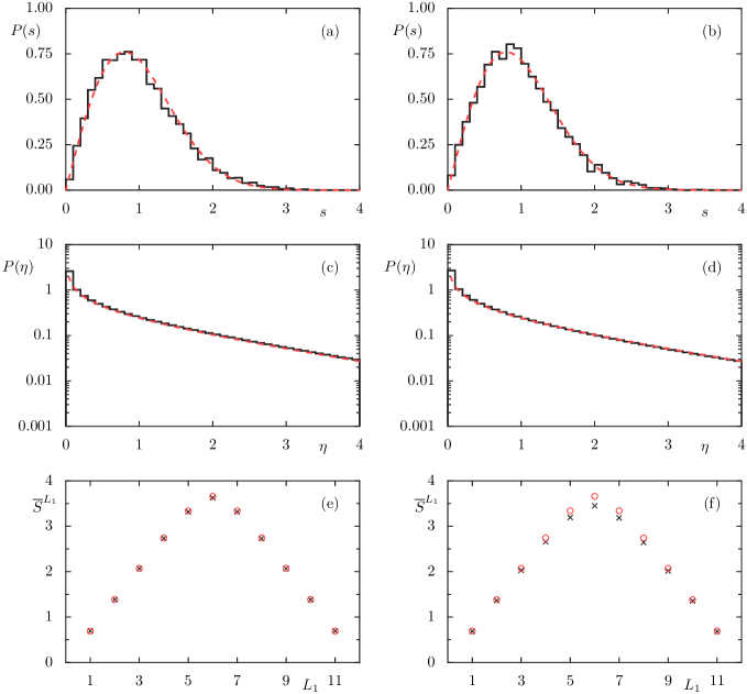
Figure 1: Level spacing distribution, eigenvector statistics, and von Neumann entropy for the kicked spin chain with $L=12$. Left column show results for parameter set A, right column for parameter set B, see table 1. Red dashed lines show COE results for level spacing distribution (3) and eigenvector statistics (6). Red circles show predictions for random states (8).

As an example of a many-body system we consider the kicked Ising spin chain with open boundary conditions. It is defined by the time dependent Hamilton operator Pro2000 ; Pro2002 ; LakSub2005 ; MisLak2014 ; PinPro2007

$$H=H_{\text{free}}+H_{\text{kick}}\sum_{k=-\infty}^{\infty}\delta(t-k)\;,$$ (9)

where

$$H_{\text{free}}= J\sum_{n=1}^{L-1}\sigma^{z}_{n}\sigma^{z}_{n+1}\;,$$ (10)

$$H_{\text{kick}}= M\sum_{n=1}^{L}\left(\cos(\Theta_{n})\sigma^{x}_{n}+\sin(\Theta_{n})\sigma^{z}_{n}\right)\;.$$ (11)

Here $\sigma^{x}_{n}$ and $\sigma^{z}_{n}$ are the standard Pauli spin-matrices, see Eq. (14) below, corresponding to the $n$th spin and $L$ is the number of spins in the chain so that the dimension of the Hilbert space is $N=2^{L}$. The free evolution part $H_{\text{free}}$ contains a nearest neighbor coupling in the $z$-component with strength $J$. The kicking part $H_{\text{kick}}$ displays a magnetic field of strength $M$, which is periodically turned on and off represented by the sum over $\delta$ distributions. The magnetic field acts on all spins but the direction in which the kick is applied for the $n$th spin depends on the angle of tilt $\Theta_{n}$ in the $x-z$ plane. The kicked Ising spin chain is time reversal invariant and has a further symmetry which is called external reflection or bitreversal symmetry PinPro2007 ; KarShaLak2007 . To avoid a desymmetrization procedure we break this symmetry by choosing different angles of tilt $\{\Theta_{n}\}$ for the individual spins. This allows us to do the following numerics in the full Hilbert space of dimension $N$. We consider the following form of the time evolution operator

$$U= \;\text{e}^{-\text{i}H_{\text{free}}/2}\text{e}^{-\text{i}H_{\text{kick}}}\text{e}^{-\text{i}H_{\text{free}}/2}\;,$$ (12)

for which the eigenstates have real coefficients in the computational basis. For the numerical computations two slightly different parameter sets for chain A and B are used, see table 1.

Figure 1 shows the level-spacing distribution, the eigenvector statistics, and the von Neumann entropy for the two chains in comparison with the corresponding RMT results. In Fig. 1(a) and (b) the level spacing distribution is shown. We see that both chains provide good agreement with the COE prediction. Also, the results for the averaged ratios $\langle r\rangle$ and $\langle\tilde{r}\rangle$ are close to the results for COE: For chain A we find $\langle r\rangle_{\text{A}}=1.735\pm 0.052$ and $\langle\tilde{r}\rangle_{\text{A}}=0.5284\pm 0.0039$ and for chain B $\langle{r}\rangle_{\text{B}}=1.770\pm 0.063$ and $\langle\tilde{r}\rangle_{\text{B}}=0.5342\pm 0.0039$. These agree within one standard deviation with results for the COE stated in section II.1. Thus, both chain A and chain B qualify as quantum chaotic. Consequently, one could expect that also other more general spectral statistics and in particular eigenstate statistics and entanglement properties follow the RMT predictions.

The eigenvector statistics is shown in Fig. 1(c) and (d) where the expansion coefficients of all eigenstates of the time evolution operator (12) in the computational basis are used. The histograms of $P(\eta)$ are shown in a semi-logarithmic representation. Neither of the two chains shows a deviation from the Porter-Thomas distribution. Note that also for small values of $\eta$, very good agreement with the COE is found, see App. A.

In Fig. 1(e) and (f) the entanglement is shown for the two chains. We compute for each eigenstate the von Neumann entropy (7) between two subchains, where subchain 1 contains the first $L_{1}$ spins of the chain, i.e. $N_{1}=2^{L_{1}}$, and subchain 2 contains the other $L_{2}=L-L_{1}$ spins, i.e. $N_{2}=2^{L-L_{1}}$. From this the average entropy $\overline{S}^{L_{1}}$ of all eigenstates is obtained. The corresponding Page curve, Eq. (8), is obtained using the corresponding dimensions $N_{1}$ and $N_{2}$ (with $N_{1}$ and $N_{2}$ exchanged if $N_{1}>N_{2}$.)

Chain A agrees well with the Page curve, with some small visible deviations around $L_{1}=6$. In contrast, the entanglement of chain B is significantly smaller. As both chains qualify as quantum chaotic, and also lead to good agreement with the RMT result for the eigenvector statistics, this is unexpected. It raises the question about the origin of this different behavior for the two spin chains which we are going to address in the following section.

III Effective spin interactions

The different behavior of the entanglement for chain A and B in Fig. 1, can be explained by differences in the effective spin interactions. To quantify these, we define an effective Hamiltonian which contains these interactions. Any unitary matrix $U$ can be written as $U=\text{e}^{-\text{i}H_{\text{eff}}}$, where $H_{\text{eff}}$ is a Hermitian matrix Thus, we define the effective Hamiltonian corresponding to the unitary operator $U$ as

$$H_{\text{eff}}=\text{i}\ln(U)\;.$$ (13)

We evaluate Eq. (13) using the eigenvectors and eigenphases defined in Sec. II.1, i.e. $H_{\text{eff}}=-\sum_{n}\varphi_{n}\outerproduct{\psi_{n}}{\psi_{n}}$. To analyze the effective spin interactions we decompose the effective Hamiltonian into the spin interaction basis. This basis is given by the tensor products $\{S_{1}\otimes\dots\otimes S_{L}\}$, where $S_{n}\in\{\sigma_{x},\sigma_{y},\sigma_{z},I\}$ for $n=1,\dots,L$, with the Pauli matrices

$$\sigma_{x}={\begin{pmatrix}0&1\\ 1&0\end{pmatrix}}\;,\quad\sigma_{y}={\begin{pmatrix}0&-{\mathrm{i}}\\ {\mathrm{i}}&0\end{pmatrix}}\;,\quad\sigma_{z}={\begin{pmatrix}1&0\\ 0&-1\end{pmatrix}}$$ (14)

and the identity matrix $I$. With the Hilbert-Schmidt inner product (also called Frobenius inner product for the finite-dimenional case) one gets an orthonormal basis. Thus, we can write

$$H_{\text{eff}}=\sum\;C_{S_{1},\dots,S_{L}}\left(S_{1}\otimes\dots\otimes S_{L}\right)\;,$$ (15)

where the sum runs over all combinations $(S_{1}\otimes\dots\otimes S_{L})$ and the $4^{L}$ real coefficients $\{C_{S_{1},\dots,S_{L}}\}$ are given by

$$C_{S_{1},\dots,S_{L}}=\frac{1}{2^{L}}\text{Tr}\left(\left(S_{1}\otimes\dots\otimes S_{L}\right)H_{\text{eff}}\right).$$ (16)

Each basis matrix is a Pauli string $(S_{1}\otimes\dots\otimes S_{L})$ and represents a specific spin interaction, e.g. for $L=4$ the basis matrix $(\sigma_{x}\otimes\sigma_{x}\otimes I\otimes I)$ represents the 2-spin interaction of the first and second spin in the $x$ component and $(\sigma_{x}\otimes\sigma_{x}\otimes\sigma_{x}\otimes I)$ the 3-spin interaction of first, second and third spin in the $x$ component.

The coefficients $C_{S_{1},\dots,S_{L}}$ describe the strength of the effective spin interactions. A basis matrix containing $k$ Pauli matrices presents a $k$-spin interaction, and we call $k$ the (interaction) order of the corresponding basis matrix. Note that we only consider the number of non-trivial factors in the basis matrix, i.e. we do not discuss effects of locality or support of the basis matrix. The distribution of the coefficients corresponding to the same $k$-spin interaction order embody the effective strength of this interaction order. The only basis matrix with $k=0$ is the identity matrix of dimension $2^{L}$. Thus, the corresponding coefficient $C_{I,\dots,I}$ correspond to a global phase, and we set this coefficient to zero by considering an adjusted time evolution operator $\tilde{U}=\text{e}^{\text{i}C_{I,\dots,I}}U$, which fulfills $\tilde{C}_{I,\dots,I}=0$. In the following we omit the tilde, to simplify notation.

For systems with time reversal invariance there exists a basis in which the eigenvectors are real BroFloFreMelPanWon1981 ; HaaGnuKus2018 . This leads to a real effective Hamiltonians, see (23), so that the coefficients corresponding to imaginary basis matrices are zero. Thus, the effective Hamiltonian is fully described by the remaining $2^{L-1}(2^{L}+1)$ coefficients. We only consider these coefficients in case of systems with an antiunitary symmetry.

III.1 Effective spin interactions for random matrices

Figure 2: Distribution of the coefficients (16) for COE matrices of size $N=2^{12}$ using 10 realizations. Coefficients for $k=2,4,7,12$ spin interactions are shown in dark to light colors. For each interaction order we use 500 coefficients of each realization. The red dashed line shows the prediction (18) for the COE.

For random matrices from the COE and CUE the distribution of the coefficients (16) describing the effective spin interactions can be obtained analytically. For this we define the effective Hamiltonian corresponding to a COE matrix $U^{\text{COE}}$ by

$$H_{\text{eff}}^{\text{COE}}=\text{i}\ln(U^{\text{COE}}).$$ (17)

In analogy to the kicked spin chains we evaluate Eq. (17) using the eigenvectors and eigenphases of $U^{\text{COE}}$, which are restricted to the interval $[-\pi,\pi)$. Random matrices do not have any spin like structure, therefore all interaction orders behave identical and moreover all coefficients show the same distribution. Using this we derive in App. B that the distribution $P(C)$ of the coefficients for $N$ dimensional COE matrices is a normal distribution

$$P_{{\text{COE}}}(C)=\frac{1}{\sqrt{2\pi\sigma^{2}_{\text{COE}}}}\exp\left(-\frac{C^{2}}{2\sigma^{2}_{\text{COE}}}\right)\;,$$ (18)

with variance $\sigma^{2}_{\text{COE}}=2\pi^{2}/(3N^{2})$. Note that we find for CUE matrices the same distribution with adapted variance $\sigma^{2}_{\text{CUE}}=\pi^{2}/(3N^{2})$, see App. B.

Figure 2 compares the prediction (18) with numerical data for $N=2^{12}$ dimensional COE matrices using 10 realizations. The distributions of the coefficients corresponding to $k=2,4,7,12$ spin interactions are shown. As expected, all interaction orders behave similar and follow the predicted Normal distribution.

III.2 Effective spin interactions for kicked spin chains

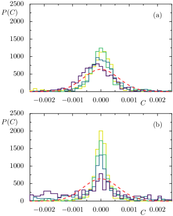
Figure 3: Distribution of the coefficients (16) for kicked spin chains of length $L=12$. (a) shows result for parameter set A, (b) for parameter set B, see table 1. Coefficients for $k=2,4,7,12$ spin interactions are shown in dark to light colors. For each interaction order 500 coefficients are used. The red dashed line shows the prediction (18) for the COE.

Now we compare the distribution of the effective spin interactions for two spin chains with the random matrix prediction, see Fig. 3. As for the COE case, we consider $k=2,4,7,12$ spin interactions.
In Fig. 3(a) we find for chain A, that the distributions for the different interaction orders are all close to the predicted COE curve. The distribution for the 2-spin interactions is slightly shifted to negative coefficients, while the larger $k$-spin interactions are centered but a bit more peaked than expected. Nevertheless, we see in particular the same distribution for all $k>2$, which is close to the RMT result and thus in line with the small deviations of the entanglement shown in Fig. 1. In contrast, Fig. 3(b) for chain B shows a clearly different behavior of the effective interactions. The distribution of the coefficients of the 2-spin interactions is broader than the predicted normal distribution. This means, that the 2-spin interactions are stronger than those of the COE. For larger $k$ the distribution becomes more and more peaked around zero, which means that these effective spin interactions are too weak in chain B. The different behavior for the individual $k$-spin interactions illustrates that we do not only find a different distribution of the interactions than expected for COE, but a fundamentally different nature of spin interactions for chain B. As a consequence, this does not allow the generation of eigenstate entanglement predicted for COE states. So the k-spin interactions, which get weaker with increasing k, explain the smaller eigenstate entanglement, found in Fig. 1 for chain B.

IV Summary, discussion, and outlook

In this paper we show, that if the level spacing distribution of a system follows RMT, the eigenstate entanglement does not necessarily show RMT results. We demonstrate this by the example of two kicked spin chains, which both qualify as quantum chaotic based on their level spacing distribution. While for both chains the eigenvector statistics follows the RMT prediction, the von Neumann entropy differs from the expected Page curve. For one chain we see the Page prediction nearly reached, but for the other the eigenstate entanglement is significantly lower. We can understand the observed entanglement by analyzing the effective $k$-spin interactions. In a random matrix situation the statitistics of the interactions behaves identical for all $k$. But for the second chain, with the smaller eigenstate entanglement, we find that the interaction reduces with increasing $k$ and thus behaves significantly different from the COE. Therefore it does not allow the creation of entanglement predicted by Page. Interestingly, we also find for the first chain, which shows only very small deviations from the Page curve, that the $k$-spin interaction statistics is slightly different from the COE result. Thus, the question arises if the deviations from RMT in the entanglement and the effective spin interactions are typical for quantum chaotic kicked spin chains. Based on the numerical explorations to find good parameter sets we have the impression that this is indeed the case for the considered kicked Ising chain. To properly decide this questions much longer chains would be required where additionally the parameter dependence seems to become less sensitive. Moreover, it would be interesting to know if this different behavior is also visible in the long-range correlations of the levels or in a more detailed analysis of the eigenvector components.

Note that deviations of the entanglement entropy from the expected RMT results were also found for the midspectrum eigenstates of autonomous spin chains BeuAndHaq2015 ; VidRig2017 ; LiuCheBal2018 ; BeuBaeMoeHaq2018 ; LeBMalVidRig2019 ; BaeHaqKha2019 including predictions and explanations for the deviations Hua2019 ; Hua2021 ; HaqClaKha2022 .

To describe the statistical properties of eigenstates of many-body systems, several RMT models have been introduced, which take the many body structure of the Hamiltonian into account. One commonly used model are the embedded random matrices FreWon1970 ; FreWon1971 ; BohFlo1971a ; BohFlo1971b ; BroFloFreMelPanWon1981 ; AsaBenRupWei2001 ; BenRupWei2001a ; GomKarKotMolRelRet2011 ; Kot2014 ; BorIzrSanZel2016 and power-law-banded random matrices KraMut1997 ; VarBra2000 ; EveMir2008 ; BogSie2018b . Another ansatz is to use random 2-spin interactions to build a random Hamiltonian KeaLinWel2015b . It would be helpful to have similar models for the unitary case. One possible approach are Floquet random unitary circuits KosLjuPro2018 ; ChaLucCha2018b ; ChaLucCha2018a ; ChaLucCha2019 ; MouPreHusCha2021 which are an extension of random unitary circuits NahRuhVijHaa2017 ; vonRakPolSon2018 to the Floquet setting and take the local structure of the time evolution operator into account by applying repeatedly the same set of random gates which couple neighboring spins. A different ansatz is based on the effective Hamiltonian (13) and its decomposition (15) into the spin interaction basis. If one can find the distribution for the coefficients corresponding to a generic kicked spin chain one can build random effective Hamiltonians $H_{\text{eff}}^{\text{random}}$ and study $U=\exp\left({-\text{i}H_{\text{eff}}^{\text{random}}}\right)$ to investigate the properties of the corresponding time evolution operator. This is an interesting task for the future.

Appendix A Logarithmic eigenvector statistics

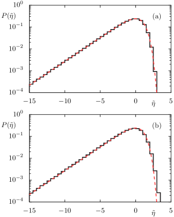
Figure 4: Distribution of $\tilde{\eta}=\ln(\eta)$ for the kicked spin chain with $L=12$. (a) shows the results for parameter set A and (b) for parameter set B, see table 1. The red dashed lines show the COE result (19).

In Fig. 1 the eigenvector distribution $P(\eta)$ is shown in a logarithmic representation, where no differences are visible between the chains A and B. To investigate the behaviour for small $\eta$ we consider the logarithm of the scaled and squared eigenvector elements $\tilde{\eta}=\ln(\eta)$. The logarithmic version of the Porter-Thomas distribution (6) reads

$$P_{\text{COE}}(\tilde{\eta})=\sqrt{\frac{\text{e}^{\tilde{\eta}}}{2\pi}}\exp\left(-\frac{\text{e}^{\tilde{\eta}}}{2}\right)\;.$$ (19)

In Fig. 4 the distribution of $\tilde{\eta}$ for chain A and chain B is shown in a logarithmic representation. For small values of $\eta$, corresponding to $\tilde{\eta}<0$, we find for both chains equally good agreement with the COE result. Interestingly, we see here for large values of $\tilde{\eta}$, that the distribution is a bit closer to the expectations for chain A than for chain B. This is in line with the deviations we see for the eigenstate entanglement. Thus, this can be seen as a hint that already the distribution of the eigenvector components can show differences from the expected behavior even if the level-spacing statistics agrees well with the RMT results.

Appendix B Distribution of the coefficients

Here we derive the distribution of the coefficients (16) of the effective spin interactions for $H_{\text{eff}}^{\text{COE}}$ as defined in Eq. (17) for random matrices, based on the known distributions of individual eigenphases and eigenvector elements for COE matrices.

The effective Hamiltonian can be written in terms of the eigenphases and eigenvectors of $U$ as

$$H_{\text{eff}} =\text{i}\ln U$$ (20)

$$=\text{i}\,\mathbf{C}\mathbf{C}^{\dagger}\,\ln U\,\mathbf{C}\mathbf{C}^{\dagger}$$ (21)

$$=\text{i}\,\mathbf{C}\,\ln(\mathbf{C}^{\dagger}U\,\mathbf{C})\,\mathbf{C}^{\dagger}$$ (22)

$$=-\mathbf{C}\,\text{diag}\left(\varphi_{1},\dots,\varphi_{N}\right)\mathbf{C}^{\dagger}\;.$$ (23)

Here we use the matrix $\mathbf{C}$, which contains the eigenvector elements, $(\mathbf{C})_{nm}=c_{m}^{(n)}=\langle m|\psi_{n}\rangle$ for the computational basis $\{|m\rangle\}_{m=1,\dots,N}$. Thus, the coefficients can be computed by

$$C_{S_{1},\dots,S_{L}}=-\frac{1}{N}\text{Tr}\big{(} \left(S_{1}\otimes\dots\otimes S_{L}\right)$$

$$\times\mathbf{C}\text{diag}\left(\varphi_{1},\dots,\varphi_{N}\right)\mathbf{C}^{\dagger}\big{)}\;.$$ (24)

The simplest non-trivial form of the dependence on the phases and eigenvector elements of $U$ arises for the coefficient

$$C_{I,I,\dots,I,\sigma_{z}}=\frac{-1}{N}\sum_{n}\varphi_{n}\sum_{m}(-1)^{m-1}|c^{(n)}_{m}|^{2}\;.$$ (25)

To find the distribution of the coefficient $C_{I,I,\dots,I,\sigma_{z}}$ we would have to use the joint distribution of all eigenphases and eigenvector elements. This distribution does not have a closed analytical from. Instead we assume that the eigenphases and eigenvector elements are independent of each other. For the COE and CUE the eigenphases are uniformly distributed in $[-\pi,\pi)$, i.e.

$$P_{\text{COE/CUE}}(\varphi)=\frac{1}{2\pi}\quad\text{for}\quad\varphi\in[-\pi,\pi)\;.$$ (26)

This distribution has an average value $\overline{\varphi}=0$ and finite variance $\sigma^{2}_{\varphi}={\pi^{2}}/{3}$. In the following, each eigenvector $|\psi_{n}\rangle$ is modeled using a normalized state $|\phi_{n}\rangle$ with coefficients $c_{m}^{(n)}=\langle m|\phi_{n}\rangle$. In case of the COE the elements $c_{m}^{(n)}$ have to be real and $\eta_{nm}=N|c_{m}^{(n)}|^{2}$ follows the Porter-Thomas distribution

$$P_{\text{COE}}(\eta)=\frac{\exp(-\eta/2)}{\sqrt{2\pi\eta}}\;,$$ (27)

which has average $\overline{\eta}_{\text{COE}}=1$ and variance $\sigma^{2}_{\eta,\text{COE}}=2$. For the CUE $c_{m}^{(n)}$ can also become complex and the distribution is an exponential,

$$P_{\text{CUE}}(\eta)=\text{e}^{-\eta}\;,$$ (28)

with average $\overline{\eta}_{\text{CUE}}=1$ and variance $\sigma^{2}_{\eta,\text{CUE}}=1$.

To derive the distribution of the coefficient $C_{I,I,\dots,I,\sigma_{z}}$ we assume for simplicity that the matrix dimension $N$ is even and first discuss the sum over $m$,

$$\Sigma_{m} :=\sum_{m}(-1)^{m-1}|c^{(n)}_{m}|^{2}$$

$$=\frac{1}{N}\sum_{m=1}^{N}(-1)^{m-1}\eta_{nm}$$

$$=\frac{1}{N}\left(\sum_{m^{\prime}=1}^{N/2}\eta_{n,2m^{\prime}}-\sum_{m^{\prime}=0}^{N/2}\eta_{n,2m^{\prime}+1}\right)$$

$$=\frac{1}{2}\left(\underbrace{\frac{1}{N/2}\sum_{m^{\prime}=1}^{N/2}\eta_{n,2m^{\prime}}}_{I_{1}}-\underbrace{\frac{1}{N/2}\sum_{m^{\prime}=0}^{N/2}\eta_{n,2m^{\prime}+1}}_{I_{2}}\right)\;.$$

The entries in both sums have the same distribution, given by Eq. (27) or Eq. (28), respectively. Applying the central limit theorem for large $N$, the distributions of $I_{1}$ and $I_{2}$ will both approach a normal distribution with average zero and variance $\sigma^{2}_{I}=\sigma_{\eta}^{2}/(N/2)$. This implies that $\Sigma_{m}=1/2(I_{1}-I_{2})$ is the scaled sum of two Gaussian random variables and thus itself a Gaussian random variable with mean $\overline{\Sigma_{m}}=0$ and variance $\sigma^{2}_{\Sigma_{m}}=\frac{1}{2^{2}}(\sigma_{I}^{2}+\sigma_{I}^{2})=\sigma^{2}_{\eta}/N$, where

$$\sigma^{2}_{\Sigma_{m},\text{COE}}=2/N\;,\quad\sigma^{2}_{\Sigma_{m},\text{CUE}}=1/N\;.$$ (29)

We can now return to the distribution of the coefficient,

$$C_{I,I,\dots,I,\sigma_{z}}=\frac{-1}{N}\sum_{n}\varphi_{n}\Sigma_{m}\;,$$ (30)

which can be interpreted as a product of two random variables which follows the joint distribution of $\varphi$ and $\Sigma_{m}$. Since the mean values $\overline{\varphi}$ and $\overline{\Sigma_{m}}$ are both zero also the mean of the joint distribution is zero. The variance is given by

$$\sigma^{2}_{\varphi\Sigma_{m}}=\sigma^{2}_{\varphi}\sigma^{2}_{\Sigma_{m}}+\sigma^{2}_{\varphi}\left(\overline{\Sigma_{m}}\right)^{2}+\sigma^{2}_{\Sigma_{m}}\left(\overline{\varphi}\right)^{2}=\frac{\pi^{2}}{3}\sigma^{2}_{\Sigma_{m}}\;.$$

Since this is a finite value we can apply the central limit theorem and find that the coefficient $C_{I,I,\dots,I,\sigma_{z}}$ follow Gaussian distribution with mean value zero and variance $\sigma^{2}=\sigma^{2}_{\varphi\Sigma_{m}}/N$. Thus, we find

$$\sigma^{2}_{\text{COE}}=\frac{\pi^{2}}{3}\frac{2}{N^{2}}\;,\quad\sigma^{2}_{\text{CUE}}=\frac{\pi^{2}}{3}\frac{1}{N^{2}}\;.$$

As discussed before this distribution holds also for all the other coefficients.

References

- (1) T. Guhr, A. Müller-Groeling, and H. A. Weidenmüller, Random-matrix theories in quantum physics: common concepts, Phys. Rep. 299, 189 (1998).
- (2) M. L. Mehta, Random Matrices, Elsevier, 3rd edition (2004).
- (3) O. Bohigas, M. J. Giannoni, and C. Schmit, Characterization of chaotic quantum spectra and universality of level fluctuation laws, Phys. Rev. Lett. 52, 1 (1984).
- (4) M. V. Berry, Semiclassical theory of spectral rigidity, Proc. R. Soc. Lon. A 400, 229 (1985).
- (5) M. Sieber and K. Richter, Correlations between periodic orbits and their rôle in spectral statistics, Phys. Scripta 2001, 128 (2001).
- (6) S. Müller, S. Heusler, A. Altland, P. Braun, and F. Haake, Periodic-orbit theory of universal level correlations in quantum chaos, New J. Phys. 11, 103025 (2009).
- (7) R. V. Jensen and R. Shankar, Statistical behavior in deterministic quantum systems with few degrees of freedom, Phys. Rev. Lett. 54, 1879 (1985).
- (8) T. C. Hsu and J. C. Anglés d’Auriac, Level repulsion in integrable and almost-integrable quantum spin models, Phys. Rev. B 47, 14291 (1993).
- (9) G. Montambaux, D. Poilblanc, J. Bellissard, and C. Sire, Quantum chaos in spin-fermion models, Phys. Rev. Lett. 70, 497 (1993).
- (10) P. Jacquod and D. L. Shepelyansky, Emergence of quantum chaos in finite interacting Fermi systems, Phys. Rev. Lett. 79, 1837 (1997).
- (11) Y. Avishai, J. Richert, and R. Berkovits, Level statistics in a Heisenberg chain with random magnetic field, Phys. Rev. B 66, 052416 (2002).
- (12) L. F. Santos, Integrability of a disordered Heisenberg spin-1/2 chain, J. Phys. A 37, 4723 (2004).
- (13) P. Ponte, Z. Papić, F. Huveneers, and D. A. Abanin, Many-body localization in periodically driven systems, Phys. Rev. Lett. 114, 140401 (2015).
- (14) V. Khemani, A. Lazarides, R. Moessner, and S. L. Sondhi, Phase structure of driven quantum systems, Phys. Rev. Lett. 116, 250401 (2016).
- (15) M. Akila, D. Waltner, B. Gutkin, and T. Guhr, Particle-time duality in the kicked Ising spin chain, J. Phys. A 49, 375101 (2016).
- (16) P. Bordia, H. Lüschen, U. Schneider, M. Knap, and I. Bloch, Periodically driving a many-body localized quantum system, Nature Physics 13, 460 (2017).
- (17) D. J. Luitz and Y. Bar Lev, The ergodic side of the many-body localization transition, Ann. Phys. 529, 1600350 (2017).
- (18) P. Kos, M. Ljubotina, and T. Prosen, Many-body quantum chaos: Analytic connection to random matrix theory, Phys. Rev. X 8, 021062 (2018).
- (19) L. F. Santos and M. Rigol, Onset of quantum chaos in one-dimensional bosonic and fermionic systems and its relation to thermalization, Phys. Rev. E 81, 036206 (2010).
- (20) L. D’Alessio and M. Rigol, Long-time behavior of isolated periodically driven interacting lattice systems, Phys. Rev. X 4, 041048 (2014).
- (21) D. J. Luitz, N. Laflorencie, and F. Alet, Many-body localization edge in the random-field Heisenberg chain, Phys. Rev. B 91, 081103(R) (2015).
- (22) E. Lubkin, Entropy of an -system from its correlation with a -reservoir, J. Math. Phys. 19, 1028 (1978).
- (23) D. N. Page, Average entropy of a subsystem, Phys. Rev. Lett. 71, 1291 (1993).
- (24) S. Sen, Average entropy of a quantum subsystem, Phys. Rev. Lett. 77, 1 (1996).
- (25) S. Kumar and A. Pandey, Entanglement in random pure states: spectral density and average von Neumann entropy, J. Phys. A 44, 445301 (2011).
- (26) E. Wigner, Random matrices in physics, SIAM Rev. 9, 1 (1967).
- (27) B. Dietz and F. Haake, Taylor and Padé analysis of the level spacing distributions of random-matrix ensembles, Z. Phys. B 80, 153 (1990).
- (28) V. Oganesyan and D. A. Huse, Localization of interacting fermions at high temperature, Phys. Rev. B 75, 155111 (2007).
- (29) Y. Y. Atas, E. Bogomolny, O. Giraud, and G. Roux, Distribution of the ratio of consecutive level spacings in random matrix ensembles, Phys. Rev. Lett. 110, 084101 (2013).
- (30) C. E. Porter and R. G. Thomas, Fluctuations of nuclear reaction widths, Phys. Rev. 104, 483 (1956).
- (31) T. A. Brody, J. Flores, J. B. French, P. A. Mello, A. Pandey, and S. S. M. Wong, Random-matrix physics: spectrum and strength fluctuations, Rev. Mod. Phys. 53, 385 (1981).
- (32) F. Haake, S. Gnutzmann, and M. Kuś, Quantum Signatures of Chaos, Springer Series in Synergetics, Springer International Publishing, Cham (2018).
- (33) T. Prosen, Exact time-correlation functions of quantum Ising chain in a kicking transversal magnetic field, Prog. Theor. Phys. Suppl. 139, 191 (2000).
- (34) T. Prosen, General relation between quantum ergodicity and fidelity of quantum dynamics, Phys. Rev. E 65, 036208 (2002).
- (35) A. Lakshminarayan and V. Subrahmanyam, Multipartite entanglement in a one-dimensional time-dependent Ising model, Phys. Rev. A 71, 062334 (2005).
- (36) S. K. Mishra and A. Lakshminarayan, Resonance and generation of random states in a quenched Ising model, Europhys. Lett. 105, 10002 (2014).
- (37) C. Pineda and T. Prosen, Universal and nonuniversal level statistics in a chaotic quantum spin chain, Phys. Rev. E 76, 061127 (2007).
- (38) J. Karthik, A. Sharma, and A. Lakshminarayan, Entanglement, avoided crossings, and quantum chaos in an Ising model with a tilted magnetic field, Phys. Rev. A 75, 022304 (2007).
- (39) W. Beugeling, A. Andreanov, and M. Haque, Global characteristics of all eigenstates of local many-body Hamiltonians: participation ratio and entanglement entropy, J. Stat. Mech. 2015, P02002 (2015).
- (40) L. Vidmar and M. Rigol, Entanglement entropy of eigenstates of quantum chaotic Hamiltonians, Phys. Rev. Lett. 119, 220603 (2017).
- (41) C. Liu, X. Chen, and L. Balents, Quantum entanglement of the Sachdev-Ye-Kitaev models, Phys. Rev. B 97, 245126 (2018).
- (42) W. Beugeling, A. Bäcker, R. Moessner, and M. Haque, Statistical properties of eigenstate amplitudes in complex quantum systems, Phys. Rev. E 98, 022204 (2018).
- (43) T. LeBlond, K. Mallayya, L. Vidmar, and M. Rigol, Entanglement and matrix elements of observables in interacting integrable systems, Phys. Rev. E 100, 062134 (2019).
- (44) A. Bäcker, M. Haque, and I. M. Khaymovich, Multifractal dimensions for random matrices, chaotic quantum maps, and many-body systems, Phys. Rev. E 100, 032117 (2019).
- (45) Y. Huang, Universal eigenstate entanglement of chaotic local Hamiltonians, Nuclear Physics B 938, 594 (2019).
- (46) Y. Huang, Universal entanglement of mid-spectrum eigenstates of chaotic local Hamiltonians, Nuclear Physics B 966, 115373 (2021).
- (47) M. Haque, P. A. McClarty, and I. M. Khaymovich, Entanglement of midspectrum eigenstates of chaotic many-body systems: Reasons for deviation from random ensembles, Phys. Rev. E 105, 014109 (2022).
- (48) J. B. French and S. S. M. Wong, Validity of random matrix theories for many-particle systems, Phys. Lett. B 33, 449 (1970).
- (49) J. B. French and S. S. M. Wong, Some random-matrix level and spacing distributions for fixed-particle-rank interactions, Phys. Lett. B 35, 5 (1971).
- (50) O. Bohigas and J. Flores, Spacing and individual eigenvalue distributions of two-body random Hamiltonians, Phys. Lett. B 35, 383 (1971).
- (51) O. Bohigas and J. Flores, Two-body random Hamiltonian and level density, Phys. Lett. B 34, 261 (1971).
- (52) T. Asaga, L. Benet, T. Rupp, and H. A. Weidenmüller, Non-ergodic behaviour of the k-body embedded Gaussian random ensembles for bosons, Europhys. Lett. 56, 340 (2001).
- (53) L. Benet, T. Rupp, and H. A. Weidenmüller, Nonuniversal behavior of the -body embedded Gaussian unitary ensemble of random matrices, Phys. Rev. Lett. 87, 010601 (2001).
- (54) J. M. G. Gómez, K. Kar, V. K. B. Kota, R. A. Molina, A. Relaño, and J. Retamosa, Many-body quantum chaos: Recent developments and applications to nuclei, Phys. Rep. 499, 103 (2011).
- (55) V. K. B. Kota, Embedded Random Matrix Ensembles in Quantum Physics, number 884 in Lecture Notes in Physics, Springer International Publishing (2014).
- (56) F. Borgonovi, F. M. Izrailev, L. F. Santos, and V. G. Zelevinsky, Quantum chaos and thermalization in isolated systems of interacting particles, Phys. Rep. 626, 1 (2016).
- (57) V. E. Kravtsov and K. A. Muttalib, New class of random matrix ensembles with multifractal eigenvectors, Phys. Rev. Lett. 79, 1913 (1997).
- (58) I. Varga and D. Braun, Critical statistics in a power-law random-banded matrix ensemble, Phys. Rev. B 61, R11859 (2000).
- (59) F. Evers and A. D. Mirlin, Anderson transitions, Rev. Mod. Phys. 80, 1355 (2008).
- (60) E. Bogomolny and M. Sieber, Power-law random banded matrices and ultrametric matrices: Eigenvector distribution in the intermediate regime, Phys. Rev. E 98, 042116 (2018).
- (61) J. P. Keating, N. Linden, and H. J. Wells, Random matrices and quantum spin chains, Markov Processes and Related Fields 21, 537 (2015).
- (62) A. Chan, A. De Luca, and J. T. Chalker, Solution of a minimal model for many-body quantum chaos, Phys. Rev. X 8, 041019 (2018).
- (63) A. Chan, A. De Luca, and J. T. Chalker, Spectral statistics in spatially extended chaotic quantum many-body systems, Phys. Rev. Lett. 121, 060601 (2018).
- (64) A. Chan, A. De Luca, and J. T. Chalker, Eigenstate correlations, thermalization, and the butterfly effect, Phys. Rev. Lett. 122, 220601 (2019).
- (65) S. Moudgalya, A. Prem, D. A. Huse, and A. Chan, Spectral statistics in constrained many-body quantum chaotic systems, Phys. Rev. Res. 3, 023176 (2021).
- (66) A. Nahum, J. Ruhman, S. Vijay, and J. Haah, Quantum entanglement growth under random unitary dynamics, Phys. Rev. X 7, 031016 (2017).
- (67) C. W. von Keyserlingk, T. Rakovszky, F. Pollmann, and S. L. Sondhi, Operator hydrodynamics, OTOCs, and entanglement growth in systems without conservation laws, Phys. Rev. X 8, 021013 (2018).