Abstract

We suggest an explanation for and explore the consequences of the excess around 95 GeV in the di-photon and di-tau invariant mass distributions recently reported by the CMS collaboration at the Large Hadron Collider (LHC), together with the discrepancy that has long been observed at the Large Electron-Positron (LEP) collider in the $b\bar{b}$ invariant mass. Interestingly, the most recent findings announced by the ATLAS collaboration do not contradict, or even support, these intriguing observations. Their search in the di-photon final state similarly reveals an excess of events within the same mass range, albeit with a bit lower significance, thereby corroborating and somewhat reinforcing the observations made by CMS. We have found that all three signatures can be explained within the general 2-Higgs Doublet Model (2HDM) Type-III. We demonstrate that the lightest CP-even Higgs boson in this scenario can explain the excess in all three channels simultaneously, i.e., in the di-photon, di-tau and $b\bar{b}$ mass spectra, while satisfying up-to-date theoretical and experimental constraints. Moreover, the 2HDM Type-III predicts an excess in the $pp\to t\bar{t}H_{\rm SM}$ production channel of the 125 GeV Higgs boson discovered in 2012, with properties (couplings, spin and CP quantum numbers) consistent with those predicted in the Standard Model (SM). This effect is caused by a up to 18% enhancement of the Yukawa coupling to top (anti)quarks in comparison to the SM value. Such an effect can be tested soon at the High Luminosity LHC (HL-LHC), which can either discover or exclude the scenario we suggest. This unique characteristic of the 2HDM Type-III makes this scenario with the 95 GeV resonance very attractive for further theoretical and experimental investigations at the (HL-)LHC and future colliders.

1 Introduction

In the last ten years, a great amount of effort has been put into the precise determination of the properties of the Higgs boson, following its discovery at the Large Hadron Collider (LHC) in 2012 [1, 2]. Many such properties are now established with accuracies better than 10% and most of the experimental observations made up to date are consistent with the Standard Model (SM) expectations. Nevertheless, current precision Higgs physics at the LHC provides room for the possibility to go Beyond the SM (BSM) in search of additional Higgs states besides the SM-like one, with masses ranging from a few GeV up to the TeV scale. Many well-motivated BSM scenarios with extended Higgs sectors, either fundamental (e.g., various Supersymmetric models [3]) or effective ones (e.g., 2-Higgs Doublet Models (2HDMs) [4, 5]), predict the existence of extra light and heavy Higgs bosons, thus motivating searches for these non-standard (pseudo)scalar states at various lepton and hadron colliders.

The 2HDM is one of the most well-studied BSM scenarios where the SM Higgs sector is extended by one additional Higgs doublet. In the most generic version of the 2HDM, the Yukawa couplings are non-diagonal in flavour space since each of the two Higgs doublets couple to all the SM fermions simultaneously. As a consequence, unwanted tree-level Flavour Changing Neutral Currents (FCNCs) may be induced, contradicting experimental observations. To tackle this problem, usually a $Z_{2}$ symmetry is imposed on the model that determines in turn the coupling structure of the two Higgs doublets to the SM fermions, so that the 2HDM can be classified into the so-called Type-I, Type-II, lepton-specific and flipped scenarios [5]. However, there is another possibility, i.e., the 2HDM Type-III where, instead of introducing such a $Z_{2}$ symmetry, one allows for simultaneous couplings of the two Higgs doublets to all SM fermions. The generic Yukawa structure resulting from such a configuration can be constrained using various theoretical requirements of self-consistency of the model as well as a range of experimental measurements of the Higgs masses and couplings present in the model.

In the ongoing search for a low-mass Higgs boson, the CMS collaboration reported in 2018 an excess in the invariant mass of di-photon events near 95 GeV [6]. In March 2023, CMS has released their latest results, confirming the excess by employing advanced analysis techniques and utilising data collected during the first, second and third years of Run 2, corresponding to integrated luminosities of 36.3 fb^-1, 41.5 fb^-1 and 54.4 fb^-1, respectively, all at a center-of-mass energy of 13 TeV [7]. The combined data exhibited an excess with a local significance of 2.9$\sigma$ at a mass of $m_{\gamma\gamma}=95.4$ GeV.

The ATLAS collaboration recently released their findings in this channel derived from the full Run 2 data set [8]. Notably, their latest analysis showcases a significantly enhanced level of sensitivity compared to their previous study, which relied on only 80 fb^-1 of data [9]. In their updated analysis, ATLAS reveals an excess with a local significance of 1.7$\sigma$ in the $\gamma\gamma$ channel around an invariant mass of 95 GeV, remarkably aligning with the reported CMS observation.

Furthermore, an additional excess has recently been reported by CMS in the search for a light neutral (pseudo)scalar boson $\phi$ in the production and decay process $gg,~{}b\bar{b}\to\phi\to\tau\tau$[10], with a local (global) significance of $3.1\sigma(2.7\sigma)$ for $m_{\phi}\approx 100~{}\text{GeV}$. Considering the poor resolution of $m_{\tau\tau}$ in comparison to $m_{\gamma\gamma}$, the two excesses observed in the two final states actually appear to be compatible. Previously, the Large Electron Positron (LEP) collider collaborations [11] explored the low-mass domain extensively in the $e^{+}e^{-}\to Z\phi$ production mode, with a generic Higgs boson state $\phi$ decaying via the $\tau\tau$ and $b\overline{b}$ channels. Interestingly, an excess has been reported in 2006 in the $e^{+}e^{-}\to Z{\phi}(\to b\overline{b})$ mode for $m_{b\bar{b}}$ around 98 GeV [12]. Given the limited mass resolution of the di-jet invariant mass at LEP, this anomaly may well coincide with the aforementioned excesses seen by CMS and/or ATLAS in the $\gamma\gamma$ and $\tau\tau$ final state. Since the excesses appear in very similar mass regions, several studies [13, 14, 15, 16, 17, 18, 19, 20, 21, 22, 23, 24, 25, 26, 27, 28, 29] have explored the possibility of simultaneously explaining these anomalies within BSM frameworks featuring a non-standard Higgs state lighter than 125 GeV, while being in agreement with current measurements of the properties of the $\approx 125$ GeV SM-like Higgs state observed at the LHC. In the attempt to explain the excesses in the $\gamma\gamma$ and $b\overline{b}$ channels, it was found in Refs. [30, 31] that the 2HDM Type-III with a particular Yukawa texture can successfully accommodate both measurements simultaneously with the lightest CP-even Higgs boson of the model, while being consistent with all relevant theoretical and experimental constraints. Further recent studies have shown that actually all three aforementioned signatures can be simultaneously explained in the 2HDM plus a real (N2HDM) [26] and complex (S2HDM)  [27, 29] singlet.

In the present study, we show that all three anomalies seen in the $\gamma\gamma$, $\tau\tau$ and $b\bar{b}$ final states can also be explained within the 2HDM Type-III of Refs. [30, 31], thereby making the point that one does not need to go beyond the minimal 2HDM framework. Moreover, in our study, we obtain an important prediction from the 2HDM Type-III configuration explaining the anomalous data, namely, we predict an enhancement of the $gg,q\bar{q}\to t\bar{t}H_{\rm SM}$ production process of the SM-like Higgs, due to an increase of the Yukawa coupling of such Higgs state with top (anti)quarks, with respect to the SM, which can be tested in the near future to finally discover or exclude the scenario we suggest.

The paper is organised as follows. In section 2, we review the theoretical framework we have chosen, i.e., the 2HDM Type-III. We describe the three excesses observed at LEP and the LHC in section 3. In section 4, we outline the relevant theoretical and experimental constraints considered in this analysis. In section 5, we present our numerical set-up to scan the parameter space of the 2HDM Type-III in order to find an explanation of the three anomalies and how this can be achieved, including the consequences for other Higgs processes. Finally, we conclude in section 6. (We also have an appendix with additional results.)

2 2HDM Type-III

The 2HDM includes two $SU(2)_{L}$ doublets with hypercharge $Y=1$. The most general renormalisable $SU(2)_{L}\times U(1)_{Y}$ invariant scalar potential is written as follows [5]:

$$\mathcal{V} =m_{11}^{2}\Phi_{1}^{\dagger}\Phi_{1}+m_{22}^{2}\Phi_{2}^{\dagger}\Phi_{2}-\left[m_{12}^{2}\Phi_{1}^{\dagger}\Phi_{2}+\rm{H.c.}\right]+\lambda_{1}(\Phi_{1}^{\dagger}\Phi_{1})^{2}+\lambda_{2}(\Phi_{2}^{\dagger}\Phi_{2})^{2}+\lambda_{3}(\Phi_{1}^{\dagger}\Phi_{1})(\Phi_{2}^{\dagger}\Phi_{2})~{}$$ (1)

$$+\lambda_{4}(\Phi_{1}^{\dagger}\Phi_{2})(\Phi_{2}^{\dagger}\Phi_{1})+\frac{1}{2}\left[\lambda_{5}(\Phi_{1}^{\dagger}\Phi_{2})^{2}+\rm{H.c.}\right]+\left\{\left[\lambda_{6}(\Phi_{1}^{\dagger}\Phi_{1})+\lambda_{7}(\Phi_{2}^{\dagger}\Phi_{2})\right](\Phi_{1}^{\dagger}\Phi_{2})+\rm{H.c.}\right\},$$

where $m_{11}^{2}$, $m_{22}^{2}$, $m_{12}^{2}$ are mass squared terms and $\lambda_{i}$ ($i=1,...,7$) are dimensionless quantities describing the coupling of the order-4 interactions. Of all such parameters, 6 are real ($m_{11}^{2}$, $m_{22}^{2}$ and $\lambda_{i}$ with $i=1,...,4$) and 4 are a priori complex ($m_{12}^{2}$ and $\lambda_{i}$ with $i=5,...,7$). Therefore, in general, the model has 14 free parameters. Under appropriate manipulations, this number can however be reduced. Following Ref. [32], to start with, one can diagonalise the quadratic part of the potential in the $({\Phi_{1},\Phi_{2}})$ space, removing the $m_{12}^{2}$ term, thus getting rid of 2 parameters. Then, one can make a relative $U(1)$ transformation on $\Phi_{1}$ or $\Phi_{2}$, making $\lambda_{5}$ real, hence down to 11 parameters. Next, by removing CP violation, the number of free parameters reduces to 9 (this requires making one neutral Higgs state decouple from both $VV$ ($VV=W^{+}W^{-}$ and $ZZ$) and $H^{+}H^{-}$ interactions). Furthermore, the Yukawa matrices corresponding to the two doublets are not simultaneously diagonalisable, which can pose a problem, as the off-diagonal elements lead to tree-level Higgs mediated Flavour Changing Neutral Currents (FCNCs) on which severe experimental bounds exist. The Glashow-Weinberg-Paschos (GWP) theorem [33, 34] states that this type of FCNCs is absent if at most one Higgs multiplet is responsible for providing mass to fermions of a given electric charge. This GWP condition can be enforced by a discrete ${Z}_{2}$-symmetry ($\Phi_{1}\rightarrow+\Phi_{1}$ and $\Phi_{2}\rightarrow-\Phi_{2}$) on the doublets, in which case the absence of FCNCs is natural. However, the need to allow for a softly broken ${Z}_{2}$-symmetry (in turn re-introducing a small $m^{2}_{12}$), as customarily done to enable Electro-Weak Symmetry Breaking (EWSB) compliant with experimental measurements, relies on the existence of a basis where $\lambda_{6}=\lambda_{7}$ = 0. As a consequence, altogether, one loses 2 parameters ($\lambda_{6}$ and $\lambda_{7}$) but regains 1 ($m^{2}_{12}$), thus reducing further their overall number down to 8. Then, after EWSB has taken place, each scalar doublet acquires a Vacuum Expectation Value (VEV) that can be parametrised as follows:

$$\langle\Phi_{1}\rangle=\frac{v}{\sqrt{2}}\begin{pmatrix}0\\ \cos\beta\end{pmatrix}\quad\quad\langle\Phi_{2}\rangle=\frac{v}{\sqrt{2}}\begin{pmatrix}0\\ \sin\beta\end{pmatrix},$$ (2)

where the angle $\beta$ determines the ratio of the two doublet VEVs, $v_{1}$ and $v_{2}$, as $\tan\beta=v_{2}/v_{1}$, and where $v=246$ GeV is a fixed value, thereby giving a final count of 7 free parameters, which we choose to be:

$$m_{h},~{}~{}m_{H},~{}~{}m_{A},~{}~{}m_{H^{\pm}},~{}~{}\sin(\beta-\alpha),~{}~{}\tan\beta,~{}~{}m^{2}_{12},$$ (3)

where $\alpha$ is the mixing angle in the CP-even Higgs sector, $m_{H}$ and $m_{h}$ denote the two CP-even Higgs masses (with $m_{h}<m_{H}$ and where either of these can be the discovered SM-like Higgs state $H_{\rm SM}$) whereas $m_{H^{\pm}}$ and $m_{A}$ are the masses of the charged and CP-odd Higgs states, respectively. (In the remainder, we will use the short-hand notation $s_{x}$ and $c_{x}$ in place of $\sin(x)$ and $\cos(x)$.)

In the Yukawa sector, the general scalar to fermions couplings are given by:

$$-{\cal L}_{Y} = \bar{Q}_{L}Y^{u}_{1}U_{R}\tilde{\Phi}_{1}+\bar{Q}_{L}Y^{u}_{2}U_{R}\tilde{\Phi}_{2}+\bar{Q}_{L}Y^{d}_{1}D_{R}\Phi_{1}+\bar{Q}_{L}Y^{d}_{2}D_{R}\Phi_{2}$$ (4)

$$+ \bar{L}Y^{\ell}_{1}\ell_{R}\Phi_{1}+\bar{L}Y^{\ell}_{2}\ell_{R}\Phi_{2}+{\rm H.c.},$$

where $Y^{f}_{1,2}$ are $3\times 3$ Yukawa matrices and $\tilde{\Phi}_{1,2}=i\sigma_{1,2}\Phi_{1,2}^{*}$, with $\sigma_{1,2}$ being the Pauli matrices. After EWSB has taken place, one can then derive the fermion masses from Eq. (4).

Here, however, we investigate a modified version of the described 2HDM, the so-called Type-III, where neither a global symmetry is implemented in the Yukawa sector nor any alignment in flavour space is enforced. We adopt instead the Cheng-Sher ansatz [35, 36], which assumes a flavour symmetry in turn suggesting a specific texture of the Yukawa matrices, where FCNC effects are proportional to the geometric mean of the two fermion masses and dimensionless parameters $\chi_{i,j}^{f}$, such that the Yukawa couplings $Y^{f}_{n}$ from the Eq. (4) are given by

$$\left[Y_{n}^{f}\right]_{i,j}=\left[\chi_{n}^{f}\right]_{ij}\sqrt{m_{i}m_{j}}/v,$$ (5)

where $i,j=1-3$. After EWSB, the Yukawa sector can be expressed in terms of the mass eigenstates of the Higgs bosons, as follows:

$$-{\cal L}^{\rm III}_{Y} =\sum_{f=u,d,\ell}\frac{m^{f}_{j}}{v}\times\left((\xi^{f}_{h})_{ij}\bar{f}_{Li}f_{Rj}h+(\xi^{f}_{H})_{ij}\bar{f}_{Li}f_{Rj}H-i(\xi^{f}_{A})_{ij}\bar{f}_{Li}f_{Rj}A\right)$$

$$+\frac{\sqrt{2}}{v}\sum_{k=1}^{3}\bar{u}_{i}\left[\left(m^{u}_{i}(\xi^{u*}_{A})_{ki}V_{kj}P_{L}+V_{ik}(\xi^{d}_{A})_{kj}m^{d}_{j}P_{R}\right)\right]d_{j}H^{+}$$

$$+\frac{\sqrt{2}}{v}\bar{\nu}_{i}(\xi^{\ell}_{A})_{ij}m^{\ell}_{j}P_{R}\ell_{j}H^{+}+{\rm H.c.}\,,$$ (6)

where the $(\xi^{f}_{\phi})_{ij}$ couplings are given in Tab. 1 in terms of the free parameters $\chi_{ij}^{f}$, $\tan\beta$ and the mixing angle $\alpha$. These expressions encompass the Higgs-fermion interactions of 2HDM Type-II together with a contribution coming from the Yukawa texture.

$\phi$	$(\xi^{u}_{\phi})_{ij}$	$(\xi^{d}_{\phi})_{ij}$	$(\xi^{\ell}_{\phi})_{ij}$
$h$	$\frac{c_{\alpha}}{s_{\beta}}\delta_{ij}-\frac{c_{\beta-\alpha}}{\sqrt{2}s_{\beta}}\sqrt{\frac{m^{u}_{i}}{m^{u}_{j}}}\chi^{u}_{ij}$	$-\frac{s_{\alpha}}{c_{\beta}}\delta_{ij}+\frac{c_{\beta-\alpha}}{\sqrt{2}c_{\beta}}\sqrt{\frac{m^{d}_{i}}{m^{d}_{j}}}\chi^{d}_{ij}$	$-\frac{s_{\alpha}}{c_{\beta}}\delta_{ij}+\frac{c_{\beta-\alpha}}{\sqrt{2}c_{\beta}}\sqrt{\frac{m^{\ell}_{i}}{m^{\ell}_{j}}}\chi^{\ell}_{ij}$
$H$	$\frac{s_{\alpha}}{s_{\beta}}\delta_{ij}+\frac{s_{\beta-\alpha}}{\sqrt{2}s_{\beta}}\sqrt{\frac{m^{u}_{i}}{m^{u}_{j}}}\chi^{u}_{ij}$	$\frac{c_{\alpha}}{c_{\beta}}\delta_{ij}-\frac{s_{\beta-\alpha}}{\sqrt{2}c_{\beta}}\sqrt{\frac{m^{d}_{i}}{m^{d}_{j}}}\chi^{d}_{ij}$	$\frac{c_{\alpha}}{c_{\beta}}\delta_{ij}-\frac{s_{\beta-\alpha}}{\sqrt{2}c_{\beta}}\sqrt{\frac{m^{\ell}_{i}}{m^{\ell}_{j}}}\chi^{\ell}_{ij}$
$A$	$\frac{1}{t_{\beta}}\delta_{ij}-\frac{1}{\sqrt{2}s_{\beta}}\sqrt{\frac{m^{u}_{i}}{m^{u}_{j}}}\chi^{u}_{ij}$	$t_{\beta}\delta_{ij}-\frac{1}{\sqrt{2}c_{\beta}}\sqrt{\frac{m^{d}_{i}}{m^{d}_{j}}}\chi^{d}_{ij}$	$t_{\beta}\delta_{ij}-\frac{1}{\sqrt{2}c_{\beta}}\sqrt{\frac{m^{\ell}_{i}}{m^{\ell}_{j}}}\chi^{\ell}_{ij}$

Table 1: Yukawa interactions in the 2HDM Type-III.

Based on the arguments presented above, the fundamental components of the Yukawa sector can be obtained in terms of the $\chi_{ij}^{f}$ parameters. These are additional free parameters of the model which describe masses and mixings of the quarks and leptons. It is crucial to ensure that rare decays, which are suppressed in the SM, do not exceed current bounds, though. Specifically, it is important to investigate the contributions of Higgs bosons to FCNC processes in $B$ mesons. Here, the non-diagonal terms are not considered and the constraints from $\Delta B=2$ processes can be ignored due to the suppression factor $\sqrt{m^{f}_{j}m^{f}_{i}}/v$. However, our analysis takes into account transitions involving $\Delta B=1$ processes. The loop transition $b\to s\gamma$ is also sensitive to BSM physics, as deviations from the currently measured rate and SM predictions could indicate the presence of a light charged Higgs boson with appropriate Yukawa couplings. Finally, since $\rm{CP}$ violation is not observed in the lepton sector, it is reasonable to assume that the $\chi_{ij}$’s are real numbers and the ensuing matrix is symmetric. However, the presence of these terms could also modify FCNCs in the Higgs sector, particularly $h\to f_{i}\bar{f_{j}}$ processes, which are proportional to non-diagonal matrix terms [36, 39], so corresponding constraints need to be enforced.

In the presence of the $\chi^{f}_{ij}$ texture parameters, alongside the standard 2HDM inputs of Eq. (3), we will start our analysis by testing the 2HDM Type-III against theoretical and current experimental constraints, which we do in the forthcoming section.

3 The Excesses in $h\to\gamma\gamma,~{}\tau\tau$ and $b\bar{b}$ Channels

In this section, we investigate whether the 2HDM Type-III can describe consistently the excess observed by both LEP and the LHC at 94–100 GeV in the $\gamma\gamma$, $\tau\tau$ and $b\overline{b}$ channels. The evaluation of the so-called ‘signal strengths’ for these excesses was done in the Narrow Width Approximation (NWA), in terms of the product of the relevant production cross section ($\sigma$, which at the LHC is dominated by gluon-gluon fusion and at LEP by the Bjorken channel) as well as decay Branching Ratios (${\cal BR}$s) as follows:

$$\mu_{{b\bar{b}}} = \frac{\sigma_{\rm 2HDM}(e^{+}e^{-}\to Z\phi)}{\sigma_{\rm SM}(e^{+}e^{-}\to Zh_{SM})}\times\frac{{\cal BR}_{\rm 2HDM}(\phi\to b\bar{b})}{{\cal BR}_{\rm SM}(h_{\rm SM}\to b\bar{b})}=\left|c_{\phi ZZ}\right|^{2}\times\frac{{\cal BR}_{\rm 2HDM}(\phi\to b\bar{b})}{{\cal BR}_{\rm SM}(h_{\rm SM}\to b\bar{b})},$$ (7)

$$\mu_{\mathrm{\tau\tau}} = \frac{\sigma_{\rm 2HDM}(gg\to\phi)}{\sigma_{\rm SM}(gg\to h_{\rm SM})}\times\frac{{\cal BR}_{\rm 2HDM}(\phi\to\tau\tau)}{{\cal BR}_{\rm SM}(h_{\rm SM}\to\tau\tau)}=\left|c_{\phi tt}\right|^{2}\times\frac{{\cal BR}_{\rm 2HDM}(\phi\to\tau\tau)}{{\cal BR}_{\rm SM}(h_{\rm SM}\to\tau\tau)},$$ (8)

$$\mu_{\mathrm{\gamma\gamma}} = \frac{\sigma_{\rm 2HDM}(gg\to\phi)}{\sigma_{\rm SM}(gg\to h_{\rm SM})}\times\frac{{\cal BR}_{\rm 2HDM}(\phi\to\gamma\gamma)}{{\cal BR}_{\rm SM}(h_{\rm SM}\to\gamma\gamma)}=\left|c_{\phi tt}\right|^{2}\times\frac{{\cal BR}_{\rm 2HDM}(\phi\to\gamma\gamma)}{{\cal BR}_{\rm SM}(h_{\rm SM}\to\gamma\gamma)},$$ (9)

where $c_{\phi ZZ}$ and $c_{\phi tt}$ are the $\phi$ couplings to $ZZ$ and $t\bar{t}$ (entering the LEP and LHC production modes, respectively) normalised to the corresponding SM values. The experimental measurements are expressed in terms of

$$\mu_{\gamma\gamma}^{\mathrm{exp}}=\mu_{\gamma\gamma}^{\mathrm{ATLAS+CMS}}=0.27^{+0.10}_{-0.09},\quad\quad\quad\mu_{\tau\tau}^{\mathrm{exp}}=1.2\pm 0.5,\quad\quad\quad\mu_{b\bar{b}}^{\mathrm{exp}}=0.117\pm 0.057,$$ (10)

where $h_{\rm SM}$ corresponds to a SM-like Higgs boson with a mass of $95$ GeV – the mass of the $h$ state of our interest from the 2HDM Type-III. In our analysis, we have combined the di-photon measurements from the ATLAS and CMS experiments, denoted as $\mu_{\gamma\gamma}^{\mathrm{ATLAS}}$ and $\mu_{\gamma\gamma}^{\mathrm{CMS}}$, respectively. The ATLAS measurement yields a central value of $0.21^{+0.12}_{-0.12}$ while the CMS measurement yields a central value of $0.33^{+0.19}_{-0.12}$. By doing so, we aimed at leveraging the strengths of both experiments and improve the precision of our analysis. The combined measurement, denoted as $\mu_{\gamma\gamma}^{\mathrm{ATLAS+CMS}}$, is determined by taking the average of the central values without assuming any correlation between them. To evaluate the combined uncertainty we sum ATLAS and CMS uncertainties in quadrature.

To determine whether a simultaneous fit to the observed excesses is possible, a $\chi^{2}$ analysis is performed using measured central values $\mu^{\mathrm{exp}}$ and the 1$\sigma$ uncertainties $\Delta\mu^{\mathrm{exp}}$ of the signal rates related to the two excesses as defined in Eqs. (7)–(9). The contribution to the $\chi^{2}$ value for each channel ($\gamma\gamma$, $\tau\tau$, $b\bar{b}$) is calculated using the formula

$$\chi^{2}_{\gamma\gamma,\tau\tau,b\bar{b}}=\frac{\left(\mu_{\gamma\gamma,\tau\tau,b\bar{b}}-\mu_{\gamma\gamma,\tau\tau,b\bar{b}}^{\mathrm{exp}}\right)^{2}}{\left(\Delta\mu^{\mathrm{exp}}_{\gamma\gamma,\tau\tau,b\bar{b}}\right)^{2}}.$$ (11)

So, the resulting $\chi^{2}$ which we will use to judge whether the points from the model describe the excess in three channels, reads as:

$$\chi^{2}_{\gamma\gamma+\tau\tau+b\bar{b}}=\chi^{2}_{\gamma\gamma}+\chi^{2}_{\tau\tau}+\chi^{2}_{b\bar{b}}.$$ (12)

In particular, we dismiss points with $\chi^{2}_{\gamma\gamma+\tau\tau+b\bar{b}}$ above 8.02, corresponding to $2\sigma$ exclusion at 95.45% C.L. for 3 degrees of freedom.

4 Theoretical and Experimental Constraints

In our study we use a comprehensive set of theoretical and experimental constraints that must be satisfied to establish a viable model.

4.1 Theoretical Constraints

In our study we impose the following set of the theoretical constraints on the scalar potential.

• Unitarity: The scattering processes involving (pseudo)scalar-(pseudo)scalar, gauge-gauge and/or (pseudo)scalar-gauge initial and/or final states must satisfy unitarity constraints. The eigenvalues $e_{i}$ of the tree-level 2-to-2 body scattering matrix should meet the following criteria: $|e_{i}|<8\pi$  [40, 41].

• Perturbativity: Adherence to perturbativity constraints imposes an upper limit on the quartic couplings of the Higgs potential: $|\lambda_{i}|<8\pi$  [5].

• Vacuum Stability: The scalar potential must be positive and bounded from below in any direction of the fields $\Phi_{i}$ to ensure vacuum stability. This requires that $\lambda_{1}>0$, $\lambda_{2}>0$, $\lambda_{3}>-\sqrt{\lambda_{1}\lambda_{2}}$, and $\lambda_{3}+\lambda_{4}-|\lambda_{5}|>-\sqrt{\lambda_{1}\lambda_{2}}$  [42, 43].

4.2 Experimental Constraints

We also apply a variety of experimental constraints from EW Precision Observables (EWPOs), measurements of the observed Higgs boson properties at the LHC, lack of signals from non-SM-like Higgs bosons at LEP, Tevatrron and LHC as well as flavour observables, which include the following.

• EWPOs: We require a $95\%$ C.L. in matching the global fit results of the EW oblique parameters $S,T$ and $U$ [44, 45] with the following values [46]:

  $$S=0.05\pm 0.08,\quad T=0.09\pm 0.07,\quad\rho_{ST}=0.92~{}~{}(\mathrm{for}~{}U=0).\hskip 42.67912pt$$

• SM-like Higgs Boson Discovery:

  We made sure that the points from our parameter space agree with the experimental measurement of the properties of the discovered SM-like Higgs boson with mass of $\approx 125$ GeV. To do this we have used public code HiggsSignals 2.6.1 [47] to evaluates a $\chi^{2}$ measure to check how the Higgs signal strengths from Tevatron and LHC are compatible with the model predictions.

• Non-SM-like Higgs Boson Exclusions: To further scrutinise the parameter space of our 2HDM Type-III, we subject the selected parameter space points to rigorous examinations against exclusion limits derived from additional Higgs boson searches. We utilise the code HiggsBounds-5.10.2 [48] to incorporate the exclusion constraints from various experiments, including LEP, Tevatron and the LHC.

• $B$-Physics Observables: We test various $B$-physics observables against experimental data using the public code SuperIso_v4.1 [49]. The following experimental measurements are used in our analysis:

         Observable        Value        Reference        ${\cal BR}(\overline{B}\to X_{s}\gamma)|_{E_{\gamma}<1.6\mathrm{~{}GeV}}$        $\left(3.32\pm 0.15\right)\times 10^{-4}$        [50]        ${\cal BR}(B^{+}\to\tau^{+}\nu_{\tau})$        $\left(1.06\pm 0.19\right)\times 10^{-4}$        [50]        ${\cal BR}(D_{s}\to\tau\nu_{\tau})$        $\left(5.51\pm 0.18\right)\times 10^{-2}$        [50]        ${\cal BR}(B_{s}\to\mu^{+}\mu^{-})$ (LHCb)        $\left(3.09^{+0.46}_{-0.43}\right)\times 10^{-9}$        [51, 52]        ${\cal BR}(B_{s}\to\mu^{+}\mu^{-})$ (CMS)        $\left(3.83^{+0.38}_{-0.36}\right)\times 10^{-9}$        [53]        ${\cal BR}(B^{0}\to\mu^{+}\mu^{-})$ (LHCb)        $\left(1.2^{+0.8}_{-0.7}\right)\times 10^{-10}$        [51, 52]        ${\cal BR}(B^{0}\to\mu^{+}\mu^{-})$ (CMS)        $\left(0.37^{+0.75}_{-0.67}\right)\times 10^{-10}$        [53]        ${\cal BR}(K\to\mu\nu_{\mu})/{\cal BR}(\pi\to\mu\nu_{\mu})$        $0.6357\pm 0.0011$        [54]

  Table 2: Flavour physics observables and corresponding values employed in our analysis.

  By rigorously examining these $B$-physics observables against experimental constraints, we can validate the compatibility of our 2HDM Type-III with existing data and potentially uncover any deviations that could indicate new physics phenomena.

5 Explanation of the Excesses

In this section, we present our numerical analysis of the 2HDM Type-III parameter space. In doing it, we have used 2HDMC 1.8.0 [55] interfaced with HiggsBounds and HiggsSignal to take into account the various constraints discussed in the previous section. In accordance with the above discussions, we consider the scenario where the heavier CP-even Higgs boson $H$ is the SM-like Higgs particle $H_{\rm SM}$ discovered at the LHC with $m_{H_{\rm SM}}\approx$ 125 GeV. In this scenario the lighter CP-even Higgs, $h$, is the source of the observed excess in $\gamma\gamma$, $\tau\tau$ and $b\bar{b}$ channels around 95 GeV, which we previously labelled $h_{\rm SM}$. First, we performed an extensive scan across a wide range of model parameters to identify the optimal parameter ranges outlined in Tab. 3. These ranges have been carefully determined in accordance with all the constraints discussed in the previous section. This comprehensive scan allowed us to identify the parameter space which explains the observed excess in all three channels simultaneously at a 2$\sigma$ C.L. or better. Then we have run a dedicated scan over the reduced parameter space from Tab. 3 relevant to the explanation of the excesses in the $\gamma\gamma$, $\tau\tau$ and $b\bar{b}$ channels for $m_{h}$ around 95 GeV.

$m_{h}$ $m_{H}$ $m_{A}$ $m_{H^{\pm}}$ $s_{\beta-\alpha}$ $\tan\beta$ $m_{12}^{2}$ $\chi_{ij}^{f,\ell}$ $[94;\,98.5]$ $125.09$ $[80;\,100]$ $[160;\,200]$ $[-0.28;\,-0.21]$ $[1;\,4]$ $m_{h}^{2}\tan\beta/(1+{\tan^{2}\beta})$ $[-3;\,3]$

Table 3: Scan ranges of the 2HDM Type-III input parameters. Masses are given in GeV.

As mentioned in the previous section, using the HiggsSignals package, we have evaluated the $\chi^{2}$ measure to judge the model compatibility with the 125 GeV Higgs boson data, which we denote as $\chi^{2}_{125}$. From the scan of the parameter space of our interest we have found $\chi^{2}_{\mathrm{125\,min}}=97.22$, the minimum value of ${\chi^{2}_{125}}$. Taking into account the number of observables, $n_{\rm obs}=107$, from HiggsSignals, which for the $\chi^{2}_{125}$ measure coincides with the Number of Degrees of Freedom, (NDF), one finds ${\chi^{2}}_{\mathrm{125\,min}}/{\rm NDF}=0.90$ (the reduced value of $\chi^{2}$), which indicates a good level of compatibility of the parameter space at $\chi^{2}_{\mathrm{125\,min}}$ with the Higgs boson data. Then we explore the parameter space around this minimum and evaluate

$$\Delta\chi^{2}_{125}=\chi^{2}_{125}-\chi^{2}_{\mathrm{125\,min}},$$ (13)

i.e., the deviation of $\chi^{2}$ around the minimum, which we study in 2-dimensional (2D) planes of the signal strength parameters: ($\mu_{\tau\tau}$ - $\mu_{\gamma\gamma}$), ($\mu_{bb}$ - $\mu_{\gamma\gamma}$) and ($\mu_{\tau\tau}$ - $\mu_{bb}$). In these planes we remove points with $\Delta\chi^{2}_{125}>5.99$, which corresponds to an exclusion of the corresponding parameter space region at 95% C.L. for 2 degrees of freedom, corresponding to the dimension of the respective planes. We emphasise that this exclusion is solely based on the properties of the SM-like Higgs state.

As a next step, over the remaining parameter space, we evaluate $\chi^{2}_{\gamma\gamma+\tau\tau+b\bar{b}}$ as given by Eq. (12) and find its minimum, which we denote as $\chi^{2}_{\mathrm{95\,min}}$. The point in the parameter space where $\chi^{2}_{\mathrm{95\,min}}$ takes place yields a ${\chi^{2}_{125}}/n_{\rm obs}=0.96$, thereby indicating again a good level of its compatibility with the Higgs boson data.

Figure 1: The colour map of $\chi^{2}_{\gamma\gamma+\tau\tau+b\bar{b}}$ in the the ($\mu_{\tau\tau}$-$\mu_{\gamma\gamma}$)(left), ($\mu_{bb}$-$\mu_{\gamma\gamma}$)(middle) and ($\mu_{\tau\tau}$-$\mu_{bb}$)(right) planes of the signal strength parameters for 2HDM Type-III parameter space under study. The solid and dashed ellipses define the regions consistent with the excess at 1$\sigma$ and 2$\sigma$ C.L. The black and red contours are for $\chi^{2}$ constructed using $\mu_{\gamma\gamma}^{\mathrm{CMS}}$ and $\mu_{\gamma\gamma}^{\mathrm{CMS+ATLAS}}$ signal strength respectively. Positions of $\chi^{2}_{95\mathrm{min}}$ and $\chi^{2}_{125\mathrm{min}}$ are indicated by green and magenta stars respectively.

(In the following we will refer to the $h$ and $H$ states of the 2HDM Type-III by using the labels ‘$h_{95}$’ and ‘$h_{125}$’, respectively.)

In Fig. 1, we present the results for $\chi^{2}_{\gamma\gamma+\tau\tau+b\bar{b}}$ in the form of its colour map projected into the ($\mu_{\tau\tau}$-$\mu_{\gamma\gamma}$) (left), ($\mu_{bb}$-$\mu_{\gamma\gamma}$) (middle) and ($\mu_{\tau\tau}$-$\mu_{bb}$) (right) planes of the signal strength parameters. All points satisfy $\chi^{2}_{\gamma\gamma+\tau\tau+b\bar{b}}\leq 8.02$ criterium required to describe an excess, the rest is excluded at 2$\sigma$ level. The solid and dashed ellipses define the regions consistent with the excess at 1$\sigma$ and 2$\sigma$ C.L., respectively, described by the $\chi^{2}_{x}+\chi^{2}_{y}=2.30$ and $\chi^{2}_{x}+\chi^{2}_{y}=6.18$ equations, where the subscripts $x$ and $y$ label each possible pairing out of three signal channels ($\gamma\gamma$, $\tau\tau$ and $b\bar{b}$), depending on the frame of Fig. 1. The black and red contours are for the $\chi^{2}$ constructed using the $\mu_{\gamma\gamma}^{\mathrm{CMS}}$ and $\mu_{\gamma\gamma}^{\mathrm{CMS+ATLAS}}$ signal strengths, respectively. Here, one can see that the green star, which indicates the position of the $\chi^{2}_{95\,\mathrm{min}}$ is inside of all 1$\sigma$ C.L. contours for each pair of signal strengths, meaning that the best point from our scan successfully describes the excess in all three channels simultaneously. This is our key result. Moreover, there are a lot of points around $\chi^{2}_{95\,\mathrm{min}}$ that are also inside 1$\sigma$ C.L. contours, in turn indicating the power of the 2HDM Type-III in general to explain the observed excess in all three channels simultaneously. The point where $\chi^{2}_{\mathrm{125\,min}}$ takes place is denoted by a magenta star.

The colour map of $\chi^{2}_{\gamma\gamma+\tau\tau+b\bar{b}}$ clearly indicates that the majority of the data points lie within the 1$\sigma$ C.L., i.e., below the threshold set by $\lesssim 3.53$, which corresponds to 2$\sigma$ C.L. for 3 degrees of freedom and one can recognise those points by their dark blue colour. One can also note from the middle and right frames of Fig. 1 that the majority of the points are situated close to the boundary of the 1$\sigma$ ellipse. This implies that, although $\mu_{\gamma\gamma}$ and $\mu_{\tau\tau}$ can be significantly large, it is slightly more difficult to achieve large values of $\mu_{b\bar{b}}$ satisfying the three constraints simultaneously. This is not surprising since satisfying the CMS $\gamma\gamma$ excess requires the $h_{95}b\bar{b}$ coupling to be small, in turn suppressing ${\cal BR}(h_{95}\to b\bar{b})$. In fact, at fixed $\Gamma_{\gamma\gamma}$ and $\Gamma_{\tau\tau}$, in order to explain the di-photon and di-tau excesses, one needs to reduce $\Gamma_{\rm tot}$, i.e., $\Gamma_{b\bar{b}}$, via a reduced Yukawa, which in turn makes ${\cal BR}(h_{95}\to b\bar{b})$ smaller. It is also observed from the right plot that $\chi^{2}_{\gamma\gamma+\tau\tau+b\bar{b}}$ exhibits lower values around the medium range of $\mu_{\tau\tau}$ (i.e., around the central value). Indeed, the decay channel $h_{95}\to\tau\tau$ has a large ${\cal BR}$ which would compete with $h_{95}\to b\overline{b}$, leading then to a large value of the $h_{95}VV$ coupling in order to fit the $b\overline{b}$ excess and to enhance the $\gamma\gamma$ one, thus lowering the values of $\chi^{2}_{\gamma\gamma+\tau\tau+b\overline{b}}$.

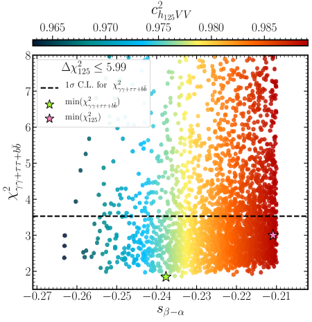
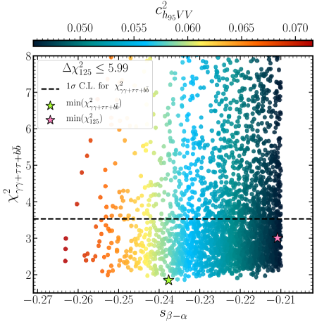
Figure 2: The $\chi^{2}_{\gamma\gamma+\tau\tau+b\bar{b}}$ dependence upon $s_{\beta-\alpha}$. The colour bar indicates the value of $c^{2}_{h_{125}VV}$ (left) and $c^{2}_{h_{95}VV}$ (right). The horizontal dashed line indicates the 1$\sigma$ region.

In Fig. 2, we show $\chi^{2}_{\gamma\gamma+\tau\tau+b\bar{b}}$ in our parameter scans as a function of $s_{\beta-\alpha}$. We also indicate the value of the Higgs couplings to SM gauge bosons, $c^{2}_{h_{125}VV}$ (left) and $c^{2}_{h_{95}VV}$ (right) in the colour bar. The horizontal dashed line represents the 1$\sigma$ region corresponding to the three excesses ($\gamma\gamma,~{}\tau\tau,~{}b\bar{b}$). The magenta and green best fit points have $\chi^{2}$ values of 1.79 and 3.05, respectively. The couplings of the $\approx 125$ GeV Higgs state, being proportional to $c_{\beta-\alpha}$, lie close to $\sim 1$. In contrast, the $c^{2}_{h_{95}VV}$ value is restricted to be quite small in the parameter region which can accommodate the three excesses.

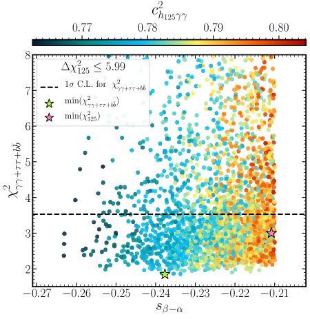
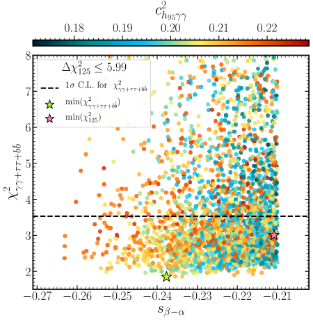
Figure 3: As in Fig. 2, but the colour coding indicates the value of $c^{2}_{h_{125}\gamma\gamma}$ (left) and $c^{2}_{h_{95}\gamma\gamma}$ (right).

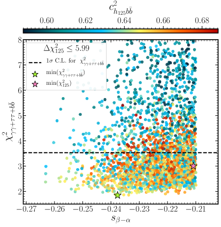
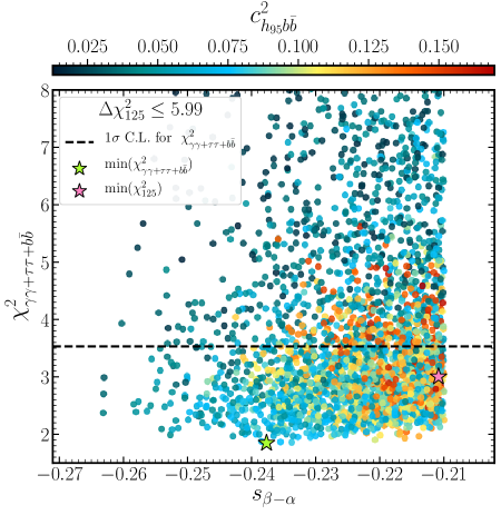
Figure 4: As in Fig. 2, but the colour coding indicates the value of $c^{2}_{h_{125}b\bar{b}}$ (left) and $c^{2}_{h_{95}b\bar{b}}$ (right).

Fig. 3 presents analogous plots to those displayed in Fig. 2. However, in this case, the colour bar represents the values of the couplings of the $\approx 125$ GeV and $\approx 95$ GeV Higgs states to $\gamma\gamma$. Clearly one can read from the left panel that, when simultaneously describing the three excesses at the 1$\sigma$ C.L., the SM-like Higgs coupling to $\gamma\gamma$ experiences a significant decrease from the predicted value in the SM with its value reaching a minimum of 0.87 and a maximum of 0.89.

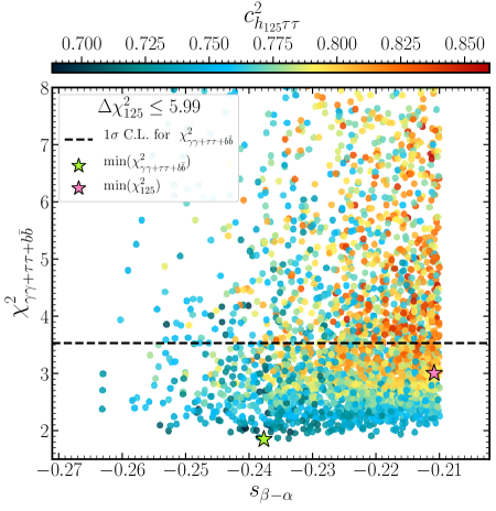
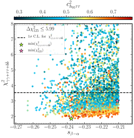
Figure 5: As in Fig. 2, but the colour coding indicates the value of $c^{2}_{h_{125}\tau\tau}$ (left) and $c^{2}_{h_{95}\tau\tau}$ (right).

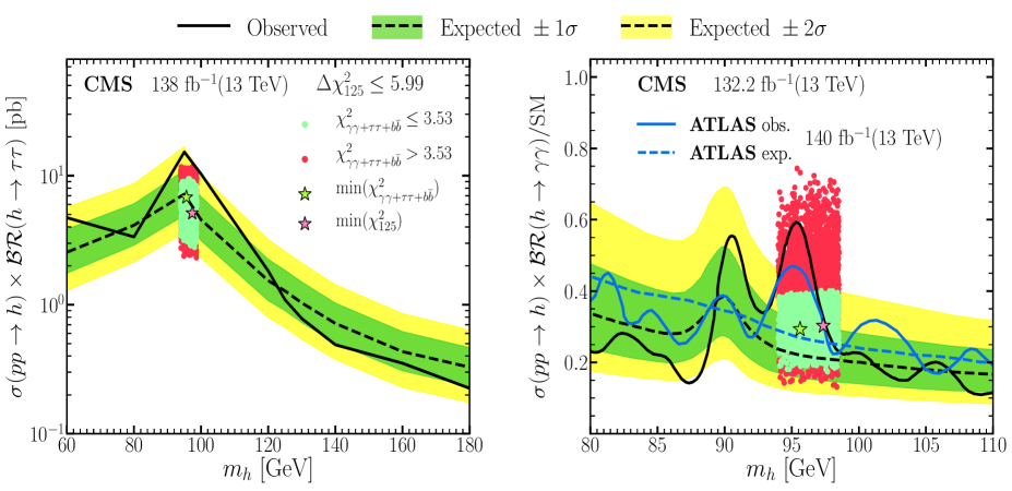
Figure 6: Allowed points, following the discussed theoretical and experimental constraints, superimposed onto the results of the CMS 13 TeV low-mass $\tau\tau$ [10] (left) and $\gamma\gamma$ [7] (right) analysis. (Notably, the right panel further includes the depiction of the ATLAS expected and observed limits from [8], showcased in blue.) The light green colour represents the parameter points that fit the excesses within a three-dimensional C.L. of 1$\sigma$ and additionally fulfil the condition $\Delta\chi^{2}_{125}\leq 5.99$, whereas the points that fit the excesses at 2$\sigma$ are shown in red in both panels.

In Fig. 4, we show similar plots as in Fig. 2, but here the colour bar depicts the values of the couplings of the 125 GeV and 95 GeV Higgs states to $b\bar{b}$. Accommodating the CMS $\gamma\gamma$ excess requires $c^{2}_{h_{95}b\bar{b}}$ to be considerably small. In contrast, the LEP $b\bar{b}$ excess prevents it to be too tiny. The balancing act between these two excesses leads to maximum values of $c^{2}_{h_{95}b\bar{b}}\sim$ 0.15 in our scans. Furthermore, $c^{2}_{h_{125}b\bar{b}}$ can reach a maximum values of $0.68$, indicating a deviation of $\sim$ 30% from the SM expectations. Thus, the precision measurement of the 125 GeV Higgs boson properties at future colliders has the potential to establish or rule out our BSM scenario as an explanation for the three excesses.

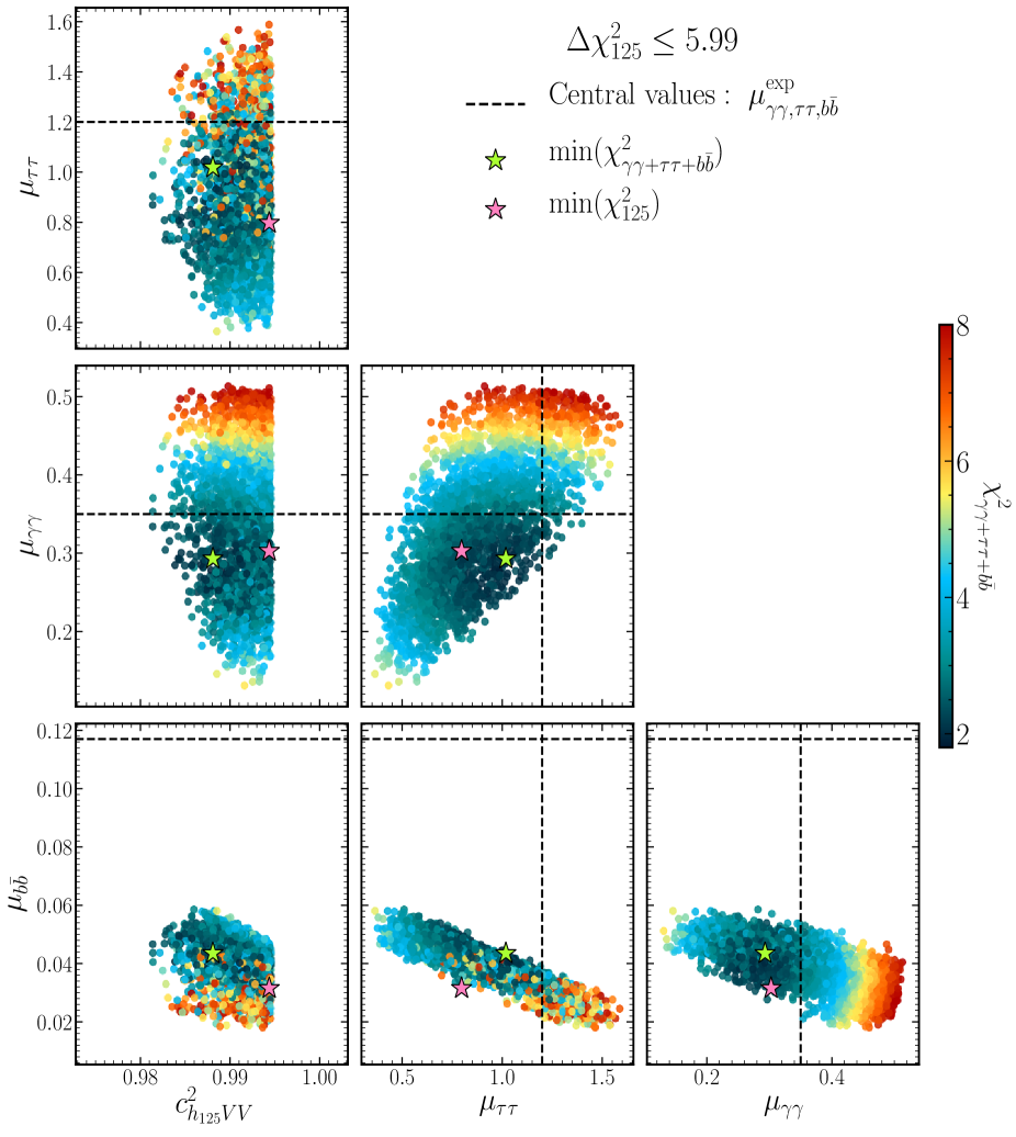
Figure 7: Correlations between $\mu_{\tau\tau}$, $\mu_{\gamma\gamma}$ and $\mu_{b\bar{b}}$ as well as the normalised coupling $c^{2}_{h_{125}VV}$. The colour bar represents $\chi^{2}_{\gamma\gamma+\tau\tau+b\bar{b}}$.(Recall that all the points satisfy the condition $\Delta\chi^{2}_{125}\leq 5.99$.)

A similar plot with the colour bar showing the $\tau\tau$ couplings of the Higgs states can be found in Fig. 5. This plot also points towards a potentially significant deviation in the SM-like Higgs boson coupling to $\tau\tau$, which can potentially be observed in upcoming collider experiments.

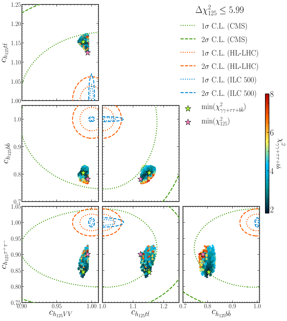
Figure 8: Correlations between pairs of $c_{h_{125}t\bar{t}}$, $c_{b_{125}t\bar{b}}$, $c_{h_{125}\tau^{+}\tau^{-}}$ and $c_{h_{125}VV}$. The colour bar represents $\chi^{2}_{\gamma\gamma+\tau\tau+b\bar{b}}$. The current $1\sigma~{}(2\sigma)$ uncertainties of the measurements of the normalised couplings $c_{h_{125}ij}$ from CMS [56] are represented by the green contours. The ellipses highlighted in orange (blue) correspond to the projected experimental precision for the normalised couplings $c_{h_{125}ij}$ at the HL-LHC [57] (International Linear Collider with $\sqrt{s}=$ 500 GeV (ILC 500)[58]) with centres located at the SM values. (Recall that all the points satisfy the condition $\Delta\chi^{2}_{125}\leq 5.99$.)

In Fig. 6, we directly compare our allowed parameter points to the experimental data by superimposing these onto the CMS 13 TeV low-mass $\tau\tau$ [10] (left) and $\gamma\gamma$ [7] (right) analysis data. The light green colour represents the parameter points that fit the excesses within a three-dimensional C.L. of 1$\sigma$ and additionally fulfil the condition $\Delta\chi^{2}_{125}\leq 5.99$, whereas the points that fit the excesses at 2$\sigma$ are shown in red. It can be clearly observed from the plots that our parameter points are exactly suited to satisfy the excesses.

In Fig. 7, we show the correlations among the signal strengths of the 95 GeV Higgs state, $\mu_{\tau\tau}$, $\mu_{\gamma\gamma}$ and $\mu_{b\bar{b}}$, against the normalised coupling $c^{2}_{h_{125}VV}$. The colour bar indicates the values of $\chi^{2}_{\gamma\gamma,\tau\tau,b\overline{b}}$. The points represent the parameter regions that fit the three excesses at the level of 1$\sigma$ and 2$\sigma$, while additionally satisfying the condition $\Delta\chi^{2}_{125}<5.99$. The dotted lines indicate the experimental central values of the excesses. One can see that both $\mu_{\tau\tau}$ and $\mu_{\gamma\gamma}$ can reach these while, in contrast, $\mu_{b\bar{b}}$ lies below the experimental central value. From the lower row, one can observe an anti-correlation between $\mu_{b\bar{b}}$ and the normalised coupling $c^{2}_{h_{125}VV}$. The small values of $\mu_{b\overline{b}}$ is due to the suppression from $h_{95}VV$. To better understand this, we recall the sum rule that implies that $\sum c^{2}_{h_{i}VV}=1$, therefore, an enhancement of $c^{2}_{h_{125}VV}$, with a deviation of less than 4% from unity, would lead to a suppression of $\mu_{b\overline{b}}\sim c^{2}_{h_{95}VV}$. Negative correlation also exists between $\mu_{b\bar{b}}$ and the other two signal strengths $\mu_{\tau\tau}$ and $\mu_{\gamma\gamma}$. This is because the latter two pose as competing decay modes to $\mu_{b\bar{b}}$. In contrast, positive correlations exist between $\mu_{\tau\tau}$ and $\mu_{\gamma\gamma}$ as can be seen from the right plot of the middle row.

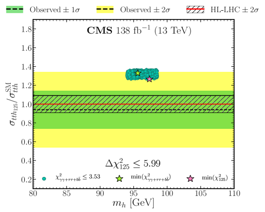
Figure 9: Predicted signal strength $\sigma_{tth_{125}}/\sigma_{tth}^{\mathrm{SM}}$ in relation to the three observed excesses. The black dashed line represents the observed value from CMS [56] while the lime green (yellow) band denotes the $1\sigma$ ($2\sigma$) range around the observed value. The hatched area illustrates the 95% probability sensitivity of the HL-LHC [57] to the normalised cross section $\sigma_{tth_{125}}/\sigma_{tth}^{\mathrm{SM}}$, centered on the value of the SM (depicted as a solid red line). Here, it is important to note that all the points adhere to the conditions $\chi^{2}_{\gamma\gamma+\tau\tau+b\bar{b}}\leq 3.53~{}\&~{}\Delta\chi^{2}_{125}\leq 5.99$.

Fig. 8 depicts the correlation between the normalised couplings of the $\approx 125$ GeV Higgs (the so-called $c_{h_{125}ij}$ parameters) in the region which accommodates the three excesses at $1\sigma$ and $2\sigma$, while being in agreement with the Higgs signal strength measurements at the LHC at $2\sigma$ ($\Delta\chi^{2}_{125}\leq 5.99$). One can see from the plot that explanation of the three excesses in $b\overline{b}$, $\tau\tau$ and $\gamma\gamma$ channels requires a large suppression of the $h_{125}b\overline{b}$ coupling which deviates by $\sim 24\%$ from the SM at $1\sigma$. In contrast, an enhancement can be seen in the Higgs coupling to $t\overline{t}$ ($c_{h_{125}t\bar{t}}$), which deviates from the SM value by $\sim 17\%$. Furthermore, the plot includes green dashed lines (solid lines) representing the current $1\sigma$ ($2\sigma$) uncertainties of the normalised couplings $c_{h_{125}i\bar{j}}$, as measured by CMS [56]. Additionally, orange and blue ellipses are depicted, illustrating the projected experimental precision for the normalised couplings at the HL-LHC [57] with an integrated luminosity of 3000 fb^-1 and the projected precision from a combination of data from the HL-LHC and ILC 500, respectively. One should bear in mind that the center of these experimental projections, for HL-LHC and ILC 500, corresponds to the SM value. Clearly, each point that simultaneously describes the three excesses is situated outside the ellipses corresponding to the HL-LHC and ILC 500. Since the points deviate significantly from the SM predictions, the expected precision of the HL-LHC and ILC 500 experiments would allow us to distinguish between the SM-like properties of $h_{125}$ and the $H$ from the 2HDM Type-III model within the parameter range that aligns with the observed excesses. Moreover, one can see that already at the HL-LHC one will be able either to discover of disprove the scenario which describes the current excess in three channels under study.

Fig. 9 illustrates the allowed parameter space in the 2HDM Type-III satisfying theoretical and experimental constraints in the $(m_{h},\sigma_{tth_{125}}/\sigma_{tth}^{\mathrm{SM}})$ plane. The black dashed line corresponds to the observed value from CMS [56] and the lime green (yellow) band represents instead the $1\sigma$ ($2\sigma$) range. The hatched area denotes the 95% C.L. probability sensitivity of the HL-LHC [57] to the normalised cross section $\sigma_{tth_{125}}/\sigma_{tth}^{\mathrm{SM}}$, centered on the SM value (solid red line). It is evident from the figure that the majority of points that simultaneously explain the three excesses fall within the 2$\sigma$ measurement range of CMS. Additionally, as seen in Fig. 8, these points exhibit an enhancement in the $h_{125}{t\bar{t}}$ coupling. In fact, due to such an enhancement, these points deviate significantly from the $2\sigma$ level of the HL-LHC projection. Note, however, that the central value used for the HL-LHC measurement corresponds to the SM prediction, i.e., 1. Thus, for points that are notably away from the SM prediction, the projected precision of the HL-LHC experiment would be sufficient to distinguish between the SM-like properties of the $h_{125}$ and the predictions of the 2HDM Type-III within the parameter space consistent with the observed enhancement in the $h_{125}{t\bar{t}}$ coupling.

In summary, there is a smoking-gun prediction stemming from our 2HDM Type-III scenario (in the configuration explaining the $\gamma\gamma,\tau\tau$ and $b\bar{b}$ anomalies), which could readily be tested at the LHC. On the one hand, $c_{h_{125}b\bar{b}}$ is consistently smaller than 1. On the other hand, $c_{h_{125}t\bar{t}}$ is consistently larger than 1. While the former condition may be difficult to test because of the uncertainties connected with $h_{125}\to b\bar{b}$ decay measurements, the latter can be accessible with good precision in production modes, not only in gluon-gluon fusion where, however, there is contamination from $b$-quark loops, but also in associated production with $t\bar{t}$ pairs, which could then be tested at the (HL-)LHC, via $pp\to t\bar{t}h_{125}$, and an ILC 500, via $e^{+}e^{-}\to t\bar{t}h_{125}$.

Finally, we conclude this section by providing a detailed overview of our best fit points in Tab. 4.

6 Conclusion

To date, large data samples have been accumulated by the LHC experiments and many analyses have been performed to examine the discussed 95 GeV excesses, following initial observations. In order to better explain the nature of these potential anomalies, a careful examination of the data, in-depth simulations and advanced computational approaches have been carried out in the literature. Along these lines, we have in this article proposed a theoretical framework, the 2HDM Type-III with a specific Yukawa texture, as a possible solution to the $\gamma\gamma$, $\tau\tau$ and $b\bar{b}$ anomalies. Specifically, we concentrated on a Higgs boson with a mass of about 95 GeV produced by gluon-gluon fusion at the 13 TeV LHC and decaying into $\tau\tau$ and $\gamma\gamma$ as well as produced by Higgs-strahlung at LEP and decaying into $b\bar{b}$.

By assuming that the heaviest CP-even Higgs state herein, $H$, is the one discovered at the LHC with mass $\approx 125$ GeV, we have identified parameter space regions where the lightest CP-even state, $h$, with a mass of $\approx 95$ GeV, can explain the observed excesses while accommodating both standard theoretical requirements of self-consistency and up-to-date experimental constraints.

Throughout this paper, we have analysed correlations amongst the signal strengths $\mu_{\gamma\gamma}$, $\mu_{\tau\tau}$ and $\mu_{b\bar{b}}$ up to the 2$\sigma$ level, arguing that the results presented are compelling and support a more extensive investigation of the proposed 2HDM Type-III scenario, by looking at processes predicted therein, which would constitute an hallmark signature of it, like $pp\to t\bar{t}H$ production, at both Run 3 of the LHC and the HL-LHC, which would be significantly enhanced with respect to the SM yield. In fact, also the study of $e^{+}e^{-}\to t\bar{t}H$ at the ILC 500, which would probe the coupling of $H$ to top (anti)quarks at the percent level, will play a crucial role in confirming the BSM construct pursued in our investigation. Thus, by incorporating the insights gained from these complementary measurements, a more comprehensive understanding of the nature of the studied excesses and the underlying theoretical framework can be achieved (assuming their persistence in future data samples at these machines).

Moreover, the anticipated precision of the HL-LHC and ILC 500 allows for effective differentiation between the SM-like characteristics of the $H$ state and the predictions of the 2HDM Type-III. This distinction is achievable for data points that display notable deviations from the SM predictions, while remaining within the parameter space that corresponds to the observed enhancement in the ${t\bar{t}}H$ coupling. Finally, one should stress that the precise measurement of the ${t\bar{t}}H$ coupling would be also very instrumental for discovery or dismissal of the proposed scenario already in the near future at the HL-LHC.

To aid such investigations, we have presented four BPs that can be used for further phenomenological studies in these directions.

Appendix

In this appendix, we provide further insights on the viability of the 2HDM Type-III as a paradigm to explain the three excesses in $\gamma\gamma$, $\tau\tau$ and $b\bar{b}$.

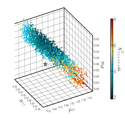
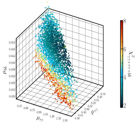
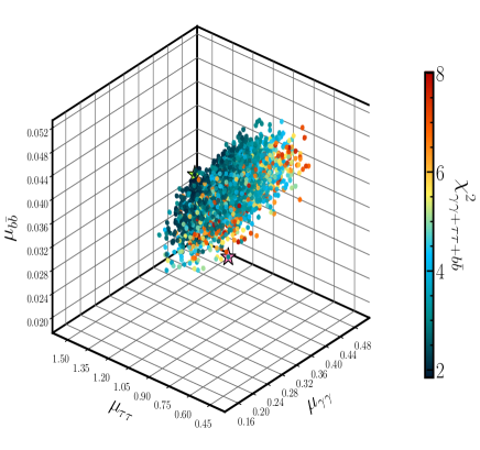
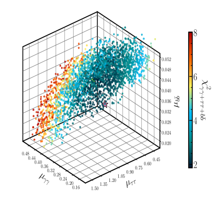
Figure 10: Same points as in Fig. 1 plotted on the 3D space with axes $\mu_{\gamma\gamma},~{}\mu_{\tau\tau}$ and $\mu_{b\bar{b}}$. The colour scheme utilised in the plot retains the same interpretation as in Fig. 1. Four visualisations of the same distribution are presented from different angles.

In Fig. 10, we present the results for $\chi^{2}_{\gamma\gamma+\tau\tau+b\bar{b}}$ by depicting its colour map projected onto the 3-Dimensional (3D) space identified by $\mu_{\gamma\gamma},\mu_{\tau\tau}$ and $\mu_{b\bar{b}}$ as axes from four distinct visualisation angles (to improve understanding of the plots). Note that the displayed data points fulfill the condition $\chi^{2}_{\gamma\gamma+\tau\tau+b\bar{b}}\leq 8.02$, indicating their ability to describe the three excesses simultaneously, at least at the 2$\sigma$ C.L. or better. Additionally, they align with the 95% C.L. measurements of the $h_{125}$ state at the LHC ($\Delta\chi^{2}_{125}\leq 5.99$), as mentioned previously. Such a figure offers a comprehensive visual representation, allowing us to explore the distribution of all our points with respect to the magenta and green stars (which retain their usual meaning). By carefully examining the 3D plot from various viewing angles, we can discern an intriguing pattern. Specifically, when the projection is made onto the $z$-axis, which corresponds to the signal strength $\mu_{b\bar{b}}$, we observe that the magenta star representing $\chi^{2}_{125\,{\rm min}}$ is notably distant from the region of high data density. Indeed, we note that the actual $\chi^{2}_{125\,{\rm min}}$ value lies close to the boundary of the viable parameter space. This observation suggests that our optimal fit is found in proximity to the edges, hence, subject to prompt experimental scrutiny with future data.

Finally, as an elaboration to what mentioned in footnote 4, we also present here Fig. 11, in order to confirm that our parameter space has been tested against the cross section limits derived from searches conducted at LEP [11] for $e^{+}e^{-}\to Zh_{95}\to Z\tau\tau$. Our scan points, the same as in Fig. 6, depicted over the $(m_{h},~{}\mathcal{\xi}^{2}\times\mathcal{BR}(h\to\tau\tau))$ 2D plane, are overlaid onto the observed and expected limits of the LEP $\tau\tau$ analyses. (The meaning of the colours is the same as in Fig. 6). Upon examination, it becomes evident that our results, describing simultaneously the three excesses, predict a cross section significantly lower than the LEP limit.

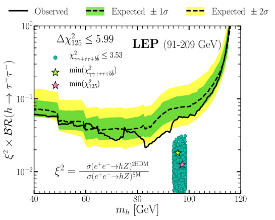
Figure 11: Same points as in Fig. 9 plotted over the $(m_{h}-\mathcal{\xi}^{2}\times\mathcal{BR}(h\to\tau^{+}\tau^{-})$ plane, superimposed onto the observed and expected limits obtained at LEP from $h_{95}\tau\tau$ searches  [11].

                  Parameters                   ★☆                   ★☆                   (Masses are in GeV)                   $m_{h}$                   97.35                   95.62                   $m_{H}$                   125.09                   125.09                   $m_{A}$                   93.98                   89.79                   $m_{H^{\pm}}$                   162.97                   162.96                   $\tan\beta$                   1.657                   1.615                   $\sin(\beta-\alpha)$                   -0.211                   -0.238                   $\chi_{11}^{u}$                   0.030                   -0.033                   $\chi_{22}^{u}$                   -0.052                   0.226                   $\chi_{33}^{u}$                   -0.153                   -0.208                   $\chi_{11}^{d}$                   0.939                   0.191                   $\chi_{22}^{d}$                   1.149                   0.339                   $\chi_{33}^{d}$                   -0.485                   -0.451                   $\chi_{11}^{\ell}$                   -0.869                   -0.383                   $\chi_{22}^{\ell}$                   -0.869                   -0.383                   $\chi_{33}^{\ell}$                   0.889                   0.760                   Effective coupling $c_{h_{i}t\bar{t}}$                   $c_{h_{95}t\bar{t}}$                   0.511                   0.541                   $c_{h_{125}t\bar{t}}$                   1.125                   1.153                   Collider signal strength                   $\mu_{\gamma\gamma}$                   0.303                   0.293                   $\mu_{\tau\tau}$                   0.797                   1.018                   $\mu_{b\bar{b}}$                   0.032                   0.044                   Total decay width in MeV                   $\Gamma(h)$                   0.333                   0.464                   $\Gamma(H)$                   4.847                   5.011                   $\Gamma(A)$                   0.852                   1.085                   $\Gamma(H^{\pm})$                   4.994                   6.388                   ${\cal BR}(h\to XY)$ in %                   ${\cal BR}(h\to\gamma\gamma)$                   0.182                   0.171                   ${\cal BR}(h\to gg)$                   12.538                   11.442                   ${\cal BR}(h\to b\bar{b})$                   55.003                   56.848                   ${\cal BR}(h\to c\bar{c})$                   5.245                   0.431                   ${\cal BR}(h\to s\bar{s})$                   0.019                   0.003                   ${\cal BR}(h\to\mu^{+}\mu^{-})$                   1.918                   0.916                   ${\cal BR}(h\to\tau\tau)$                   24.848                   29.972                   ${\cal BR}(h\to ZZ)$                   0.027                   0.024                   ${\cal BR}(h\to W^{+}W^{-})$                   0.220                   0.193                   ${\cal BR}(H\to XY)$ in %                   ${\cal BR}(H\to\gamma\gamma)$                   0.154                   0.144                   ${\cal BR}(H\to gg)$                   8.472                   8.617                   ${\cal BR}(H\to b\bar{b})$                   65.059                   66.703                   ${\cal BR}(H\to c\bar{c})$                   3.075                   2.767                   ${\cal BR}(H\to\tau\tau)$                   4.180                   3.559                   ${\cal BR}(H\to ZZ)$                   2.103                   2.008                   ${\cal BR}(H\to W^{+}W^{-})$                   16.809                   16.054                   ${\cal BR}(A\to XY)$ in %                   ${\cal BR}(A\to\gamma\gamma)$                   0.042                   0.034                   ${\cal BR}(A\to gg)$                   26.348                   22.048                   ${\cal BR}(A\to b\bar{b})$                   63.769                   69.861                   ${\cal BR}(A\to c\bar{c})$                   4.753                   1.629                   ${\cal BR}(A\to\mu\mu)$                   0.655                   0.275                   ${\cal BR}(A\to\tau\tau)$                   4.433                   6.060                   ${\cal BR}(H^{\pm}\to XY)$ in %                   ${\cal BR}(H^{\pm}\to\mu\nu)$                   0.194                   0.085                   ${\cal BR}(H^{\pm}\to cs)$                   1.129                   0.415                   ${\cal BR}(H^{\pm}\to W^{+}h)$                   25.916                   23.303                   ${\cal BR}(H^{\pm}\to W^{+}A)$                   36.613                   42.264                   ${\cal BR}(H^{\pm}\to\tau\nu)$                   1.311                   1.868                   ${\cal BR}(H^{\pm}\to tb)$                   34.612                   31.881                   $\sigma$ in [pb]                   $\sigma(pp\to h\to\gamma\gamma)$                   0.038                   0.036                   $\sigma(pp\to h\to\tau\tau)$                   5.131                   6.801

Table 4: The full description of the BPs for which the minimum value of $\chi^{2}_{\gamma\gamma+\tau\tau+b\bar{b}}$ (green star) and $\chi^{2}_{125}$ (magenta star) are found under the condition that $\Delta\chi^{2}_{125}\leq 5.99$.

References

- [1] ATLAS collaboration, Observation of a new particle in the search for the Standard Model Higgs boson with the ATLAS detector at the LHC, Phys. Lett. B 716 (2012) 1 [1207.7214].
- [2] CMS collaboration, Observation of a New Boson at a Mass of 125 GeV with the CMS Experiment at the LHC, Phys. Lett. B 716 (2012) 30 [1207.7235].
- [3] S. Moretti and S. Khalil, Supersymmetry Beyond Minimality: From Theory to Experiment, CRC Press (2019).
- [4] J.F. Gunion, H.E. Haber, G.L. Kane and S. Dawson, Errata for the Higgs hunter’s guide, hep-ph/9302272.
- [5] G.C. Branco, P.M. Ferreira, L. Lavoura, M.N. Rebelo, M. Sher and J.P. Silva, Theory and phenomenology of two-Higgs-doublet models, Phys. Rept. 516 (2012) 1 [1106.0034].
- [6] CMS collaboration, Search for a standard model-like Higgs boson in the mass range between 70 and 110 GeV in the diphoton final state in proton-proton collisions at 8 and 13 TeV, Phys. Lett. B 793 (2019) 320 [1811.08459].
- [7] CMS collaboration, Search for a standard model-like Higgs boson in the mass range between 70 and 110 in the diphoton final state in proton-proton collisions at , CMS-PAS-HIG-20-002 (2023) .
- [8] C. Arcangeletti. on behalf of ATLAS collaboration, LHC Seminar https://indico.cern.ch/event/1281604/attachments/2660420/4608571/LHCSeminarArcangeletti_final.pdf, 7th of June, 2023.
- [9] ATLAS collaboration, “Search for resonances in the 65 to 110 GeV diphoton invariant mass range using 80 fb-1 of collisions collected at TeV with the ATLAS detector.” ATLAS-CONF-2018-025, 7, 2018.
- [10] CMS collaboration, Searches for additional Higgs bosons and vector leptoquarks in final states in proton-proton collisions at , 2208.02717.
- [11] LEP Working Group for Higgs boson searches, ALEPH, DELPHI, L3, OPAL collaboration, Search for the standard model Higgs boson at LEP, Phys. Lett. B 565 (2003) 61 [hep-ex/0306033].
- [12] ALEPH, DELPHI, L3, OPAL, LEP Working Group for Higgs Boson Searches collaboration, Search for neutral MSSM Higgs bosons at LEP, Eur. Phys. J. C 47 (2006) 547 [hep-ex/0602042].
- [13] J. Cao, X. Guo, Y. He, P. Wu and Y. Zhang, Diphoton signal of the light Higgs boson in natural NMSSM, Phys. Rev. D 95 (2017) 116001 [1612.08522].
- [14] S. Heinemeyer, C. Li, F. Lika, G. Moortgat-Pick and S. Paasch, Phenomenology of a 96 GeV Higgs boson in the 2HDM with an additional singlet, Phys. Rev. D 106 (2022) 075003 [2112.11958].
- [15] T. Biekötter, A. Grohsjean, S. Heinemeyer, C. Schwanenberger and G. Weiglein, Possible indications for new Higgs bosons in the reach of the LHC: N2HDM and NMSSM interpretations, Eur. Phys. J. C 82 (2022) 178 [2109.01128].
- [16] T. Biekötter, M. Chakraborti and S. Heinemeyer, A 96 GeV Higgs boson in the N2HDM, Eur. Phys. J. C 80 (2020) 2 [1903.11661].
- [17] J. Cao, X. Jia, Y. Yue, H. Zhou and P. Zhu, 96 GeV diphoton excess in seesaw extensions of the natural NMSSM, Phys. Rev. D 101 (2020) 055008 [1908.07206].
- [18] T. Biekötter, S. Heinemeyer and G. Weiglein, Excesses in the low-mass Higgs-boson search and the -boson mass measurement, 2204.05975.
- [19] S. Iguro, T. Kitahara and Y. Omura, Scrutinizing the 95–100 GeV di-tau excess in the top associated process, Eur. Phys. J. C 82 (2022) 1053 [2205.03187].
- [20] W. Li, J. Zhu, K. Wang, S. Ma, P. Tian and H. Qiao, A light Higgs boson in the NMSSM confronted with the CMS di-photon and di-tau excesses, 2212.11739.
- [21] J.M. Cline and T. Toma, Pseudo-Goldstone dark matter confronts cosmic ray and collider anomalies, Phys. Rev. D 100 (2019) 035023 [1906.02175].
- [22] T. Biekötter and M.O. Olea-Romacho, Reconciling Higgs physics and pseudo-Nambu-Goldstone dark matter in the S2HDM using a genetic algorithm, JHEP 10 (2021) 215 [2108.10864].
- [23] A. Crivellin, J. Heeck and D. Müller, Large in generic two-Higgs-doublet models, Phys. Rev. D 97 (2018) 035008 [1710.04663].
- [24] G. Cacciapaglia, A. Deandrea, S. Gascon-Shotkin, S. Le Corre, M. Lethuillier and J. Tao, Search for a lighter Higgs boson in Two Higgs Doublet Models, JHEP 12 (2016) 068 [1607.08653].
- [25] A.A. Abdelalim, B. Das, S. Khalil and S. Moretti, Di-photon decay of a light Higgs state in the BLSSM, Nucl. Phys. B 985 (2022) 116013 [2012.04952].
- [26] T. Biekötter, S. Heinemeyer and G. Weiglein, Mounting evidence for a 95 GeV Higgs boson, JHEP 08 (2022) 201 [2203.13180].
- [27] T. Biekötter, S. Heinemeyer and G. Weiglein, The CMS di-photon excess at 95 GeV in view of the LHC Run 2 results, 2303.12018.
- [28] D. Azevedo, T. Biekötter and P.M. Ferreira, 2HDM interpretations of the CMS diphoton excess at 95 GeV, 2305.19716.
- [29] T. Biekötter, S. Heinemeyer and G. Weiglein, The 95.4 GeV di-photon excess at ATLAS and CMS, 2306.03889.
- [30] R. Benbrik, M. Boukidi, S. Moretti and S. Semlali, Explaining the 96 GeV Di-photon anomaly in a generic 2HDM Type-III, Phys. Lett. B 832 (2022) 137245 [2204.07470].
- [31] R. Benbrik, M. Boukidi, S. Moretti and S. Semlali, Probing a 96 GeV Higgs Boson in the Di-Photon Channel at the LHC, PoS ICHEP2022 (2022) 547 [2211.11140].
- [32] S. Davidson and H.E. Haber, Basis-independent methods for the two-higgs-doublet model, Phys. Rev. D 72 (2005) 035004.
- [33] S.L. Glashow and S. Weinberg, Natural conservation laws for neutral currents, Phys. Rev. D 15 (1977) 1958.
- [34] E.A. Paschos, Diagonal neutral currents, Phys. Rev. D 15 (1977) 1966.
- [35] T.P. Cheng and M. Sher, Mass Matrix Ansatz and Flavor Nonconservation in Models with Multiple Higgs Doublets, Phys. Rev. D 35 (1987) 3484.
- [36] J.L. Diaz-Cruz, R. Noriega-Papaqui and A. Rosado, Mass matrix ansatz and lepton flavor violation in the THDM-III, Phys. Rev. D 69 (2004) 095002 [hep-ph/0401194].
- [37] J. Hernandez-Sanchez, S. Moretti, R. Noriega-Papaqui and A. Rosado, Off-diagonal terms in Yukawa textures of the Type-III 2-Higgs doublet model and light charged Higgs boson phenomenology, JHEP 07 (2013) 044 [1212.6818].
- [38] A. Crivellin, A. Kokulu and C. Greub, Flavor-phenomenology of two-Higgs-doublet models with generic Yukawa structure, Phys. Rev. D 87 (2013) 094031 [1303.5877].
- [39] R. Benbrik, C.-H. Chen and T. Nomura, , , in generic two-Higgs-doublet models, Phys. Rev. D 93 (2016) 095004 [1511.08544].
- [40] S. Kanemura, T. Kubota and E. Takasugi, Lee-Quigg-Thacker bounds for Higgs boson masses in a two doublet model, Phys. Lett. B 313 (1993) 155 [hep-ph/9303263].
- [41] A.G. Akeroyd, A. Arhrib and E.-M. Naimi, Note on tree level unitarity in the general two Higgs doublet model, Phys. Lett. B 490 (2000) 119 [hep-ph/0006035].
- [42] A. Barroso, P.M. Ferreira, I.P. Ivanov and R. Santos, Metastability bounds on the two Higgs doublet model, JHEP 06 (2013) 045 [1303.5098].
- [43] N.G. Deshpande and E. Ma, Pattern of Symmetry Breaking with Two Higgs Doublets, Phys. Rev. D 18 (1978) 2574.
- [44] W. Grimus, L. Lavoura, O.M. Ogreid and P. Osland, A Precision constraint on multi-Higgs-doublet models, J. Phys. G 35 (2008) 075001 [0711.4022].
- [45] W. Grimus, L. Lavoura, O.M. Ogreid and P. Osland, The Oblique parameters in multi-Higgs-doublet models, Nucl. Phys. B 801 (2008) 81 [0802.4353].
- [46] Particle Data Group collaboration, Review of Particle Physics, PTEP 2020 (2020) 083C01.
- [47] P. Bechtle, S. Heinemeyer, T. Klingl, T. Stefaniak, G. Weiglein and J. Wittbrodt, HiggsSignals-2: Probing new physics with precision Higgs measurements in the LHC 13 TeV era, Eur. Phys. J. C 81 (2021) 145 [2012.09197].
- [48] P. Bechtle, D. Dercks, S. Heinemeyer, T. Klingl, T. Stefaniak, G. Weiglein et al., HiggsBounds-5: Testing Higgs Sectors in the LHC 13 TeV Era, Eur. Phys. J. C 80 (2020) 1211 [2006.06007].
- [49] F. Mahmoudi, SuperIso v2.3: A Program for calculating flavor physics observables in Supersymmetry, Comput. Phys. Commun. 180 (2009) 1579 [0808.3144].
- [50] HFLAV collaboration, Averages of -hadron, -hadron, and -lepton properties as of summer 2016, Eur. Phys. J. C 77 (2017) 895 [1612.07233].
- [51] LHCb collaboration, Measurement of the decay properties and search for the and decays, Phys. Rev. D 105 (2022) 012010 [2108.09283].
- [52] LHCb collaboration, Analysis of Neutral B-Meson Decays into Two Muons, Phys. Rev. Lett. 128 (2022) 041801 [2108.09284].
- [53] CMS collaboration, Measurement of the Bs0→+ decay properties and search for the B0→+ decay in proton-proton collisions at s=13TeV, Phys. Lett. B 842 (2023) 137955 [2212.10311].
- [54] LHCb collaboration, Measurement of the branching fraction and effective lifetime and search for decays, Phys. Rev. Lett. 118 (2017) 191801 [1703.05747].
- [55] D. Eriksson, J. Rathsman and O. Stal, 2HDMC: Two-Higgs-Doublet Model Calculator Physics and Manual, Comput. Phys. Commun. 181 (2010) 189 [0902.0851].
- [56] CMS collaboration, A portrait of the Higgs boson by the CMS experiment ten years after the discovery, Nature 607 (2022) 60 [2207.00043].
- [57] M. Cepeda et al., Report from Working Group 2: Higgs Physics at the HL-LHC and HE-LHC, CERN Yellow Rep. Monogr. 7 (2019) 221 [1902.00134].
- [58] P. Bambade et al., The International Linear Collider: A Global Project, 1903.01629.