Solution of a $5$-state Landau-Zener model and applications to Su-Schrieffer-Heeger chains

Abstract

We study a $5$-state Landau-Zener model which cannot be solved by integrability methods. By analyzing analytical constraints on its scattering matrix combined with fitting to results from numerical simulations of the Schrödinger equation, we find nearly exact analytical expressions of all its transition probabilities. We further apply this model to study a $5$-site Su-Schrieffer-Heeger chain with couplings changing linearly in time. Our work points out a new possibility to solve multistate Landau-Zener models not necessarily integrable and with insufficient numbers of constraints on their scattering matrices.

I Introduction

Multistate Landau-Zener (LZ) model is a class of quantum model whose Hamiltonian depends linearly on time. It is a generalization of the two-state LZ model landau ; zener ; majorana ; stuckelberg to larger numbers of levels. Unlike the two-state LZ model which is exactly solvable in the sense that its transition probabilities for an evolution from $t=-\infty$ to $t=\infty$ can be obtained in analytical forms, a general multistate LZ model cannot be exactly solved. However, at special choices of parameters, exact solvability of a multistate LZ model can be achieved; since the 1960s, different types of such models have been identified DO ; Hioe-1987 ; bow-tie ; GBT-Demkov-2000 ; GBT-Demkov-2001 ; chain-2002 ; 4-state-2002 ; 4-state-2015 ; 6-state-2015 ; DTCM-2016 ; DTCM-2016-2 ; quest-2017 ; large-class . Among them are the Demkov-Osherov model DO , the bow-tie model bow-tie , the generalized bow-tie model GBT-Demkov-2000 ; GBT-Demkov-2001 , and the driven Tavis-Cummings model DTCM-2016 ; DTCM-2016-2 ; they each present classes of solvable Hamiltonians whose number of levels can be arbitrarily large. In 2018, Sinitsyn et al. discovered that a time-dependent quantum model satisfying the so-called “integrability conditions” is integrable and may be exactly solvable commute , which provides a unified framework on studying solvable multistate LZ models. It has been shown that most of the previously discovered solvable multistate LZ models are indeed integrable, and new multistate LZ models have been studied and new solvable models been found in the light of the integrability conditions Yuzbashyan-2018 ; DSL-2019 ; MTLZ ; parallel-2020 ; quadratic-2021 ; nogo-2022 .

Integrability conditions impose strict constraints on the Hamiltonian, so a general multistate LZ model is not expected to satisfy them. Moreover, models that do satisfy the integrability conditions are not necessarily solvable, as pointed out in quadratic-2021 . However, exact solvability is also possible for certain models even without the help of integrability. For the purpose of solving such models, first, one can make use of the fact that the scattering matrix of an arbitrary multistate LZ model satisfies certain analytical constraints. In 1993, Brundolbler and Elser observed that for a general multistate LZ model, the transition probabilities to stay in the levels with extremal slopes take exact analytical forms B-E-1993 . The Brundolbler-Elser formula was later rigorously proved nogo-2004 ; Shytov-2004 , and also extended to a set of constraints on the scattering matrix of a general multistate LZ model (named the hierarchy constraints) HC-2017 . Besides, the scattering matrix of any models with a Hermitian Hamiltonian is unitary. Moreover, the specific model may possess certain symmetries which generate additional relations among its scattering amplitudes. All these together form a set of constraints on the scattering matrix, and if this set is solvable the model is also solvable. Such a method was used in HC-2017 and cross-2017 to solve several multistate LZ models (see also Nikolai-2014 on the so-called multistate Landau-Zener-Coulomb models which generalizes multistate LZ models by including terms inversely proportional to time). Since the number of unknown scattering amplitudes scales as $N^{2}$ with the number of levels $N$ and the number of constraints generally increases less fast, this analytical constraint method is generally expected to work better for models with small numbers of levels.

In this work, we consider a type of multistate LZ model which cannot be solved by integrability methods. We apply the analytical constraint method described in the previous paragraph to write out a set of constraints on its scattering matrix. We show that although this set is not solvable, the number of remaining independent unknowns is small, and for particular choices of parameters, together with results from numerical simulations we are able to express all transition probabilities by analytical functions with good accuracies. Our work thus provides a new possibility to solve a multistate LZ model without the help of integrability and when it cannot be solved directly by the constraints on its scattering matrices. We also discuss applications of our result to a $5$-site Su-Schrieffer-Heeger (SSH) model under a linear quench of its couplings.

This paper is organized as follows. In Section II, we introduce the $5$-state LZ model considered and define the scattering problem. In Section III, we analyze constraints on the scattering matrix of this model and show that all its transition probabilities depend on two independent unknowns. In Section IV, we show that, for a particular choice of parameters, these two independent unknowns can be approximately expressed by analytical expressions via fitting to exact numerical simulations. In Section V, we map the model to a $5$-site SSH chain under a linear quench and discuss its applications to the latter. Finally, Section VI presents conclusions and discussions.

II The model

The multistate LZ model we consider is the following:

$$i\frac{d\psi}{dt}=H(t)\psi,$$ (1)

$$H(t)=\left(\begin{array}[]{ccccc}-b_{1}t&g_{12}&g_{13}&g_{14}&0\\ g_{12}&-b_{2}t&0&0&-g_{14}\\ g_{13}&0&0&0&-g_{13}\\ g_{14}&0&0&b_{2}t&-g_{12}\\ 0&-g_{14}&-g_{13}&-g_{12}&b_{1}t\end{array}\right),$$ (7)

where the slopes satisfy $b_{2}>b_{1}>0$ and the couplings $g_{12}$, $g_{13}$ and $g_{14}$ are all real. This model describes interactions of two groups of levels labelled by $1,5$ and $2,3,4$, as illustrated in its connectivity graph in Fig. 1. All its diabatic energies (namely the diagonal elements of the Hamiltonian as functions of time) cross at a single point, and it thus belongs to the class of bipartite models studied in cross-2017 . Its evolution operator from an initial time $t_{i}$ to a final time $t_{f}$ can be formally written as $U(t_{f},t_{i})={\cal T}e^{-i\int_{t_{i}}^{t_{f}}H(t)dt}$, where ${\cal T}$ is a time-ordering operator. We are especially interested in the scattering matrix $S$ of an evolution from $t=-\infty$ to $\infty$, namely, $S=\lim_{T\rightarrow\infty}U(T,-T)$. The transition probability matrix $P$ is connected to $S$ by $P_{ij}=|S_{ij}|^{2}$.

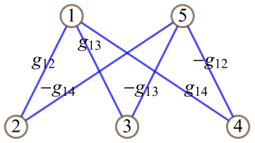
Figure 1: Connectivity graph of the model (1), with each vertex corresponding to a diabatic level and each edge to a non-zero coupling between a pair of levels. Each coupling is labelled on its corresponding edge.

One may wonder if the model (1) is integrable. We first observe that, although it has the same connectivity graph as the $5$-state “fan” model which is integrable and exactly solvable large-class ; MTLZ , it is actually not a fan model, since its order of slopes do not satisfy the constraints for a fan model large-class . It thus does not belong to multitime LZ models, because for a $5$-state LZ model the fan model is the only possibility of a multitime LZ model, as proved in nogo-2022 . Besides, we do not observe that the model can be constructed as a degenerate limit of a known integrable model with parallel levels. We also considered the Hamiltonian (7) to depend on another variable $\tau$ and looked for its commutating operator quadratic in time that satisfy integrability conditions following the procedures in quadratic-2021 . We find that such an operator does exist, but only when we allow the Hamiltonian at a general $\tau$ to violate the chiral symmetry, i.e. to allow the magnitudes of slopes of the states $1$ and $5$ to be different. In other words, the model (1) corresponds to a snapshot – a special parameter choice which respects the chiral symmetry – of a more general integrable model. But we do not find this fact helpful in solving the original model, since the underlying integrable model has lower symmetry and seems more difficult to be solved. In sum, methods on solving integrable models are not helpful in the current problem.

III Constraints on the scattering matrix

We will try to solve the model (1) by the method outlined in the second paragraph of Section I, namely, by analyzing constraints on the scattering matrix. We first notice that the model (1) possesses certain symmetries. Its Schrödinger equation is invariant under each of the following two symmetry operations (let’s write $\psi=(a_{1},a_{2},a_{3},a_{4},a_{5})^{T}$):

1. (time-reversal symmetry) $t\rightarrow-t$, and $a_{1}\rightarrow-a_{1}$, $a_{5}\rightarrow-a_{5}$;
2. (chiral symmetry) $H\rightarrow-H$, and $a_{1}\leftrightarrow a_{5}$, $a_{2}\leftrightarrow a_{4}$.

The time-reversal symmetry is a general property of a bipartite model cross-2017 . The chiral symmetry is a result of the special arrangement of the slopes and couplings in the Hamiltonian. It dictates the Hamiltonian’s adiabatic energy diagram ($E$ vs. $t$) to be symmetric under a reflection about the $E=0$ line. These two symmetries can be equivalently expressed by the following operations on the Hamiltonian:

$$H(-t)=-\Theta H(t)\Theta,$$ (8)

$$H(t)=-\Gamma H(t)\Gamma,$$ (9)

where $\Theta=\operatorname{diag}(-1,1,1,1,-1)$ is a diagonal matrix, and $\Gamma$ is an anti-diagonal matrix with all anti-diagonal elements equal to $1$. The corresponding operations on the evolution matrix $U(t_{f},t_{i})$ read:

$$\Theta U(t_{f},t_{i})\Theta=U^{\dagger}(-t_{i},-t_{f}),$$ (10)

$$\Gamma U(t_{f},t_{i})\Gamma=U^{*}(t_{f},t_{i}).$$ (11)

Taking $-t_{i}=t_{f}=T$, we find that the scattering matrix satisfies $\Theta S\Theta=S^{\dagger}$ and $\Gamma S\Gamma=S^{*}$. The most general form of $S$ satisfying these two relations is:

$$S=\left(\begin{array}[]{ccccc}S_{11}&-S_{21}^{*}&-S_{31}^{*}&-S_{41}^{*}&S_{51}^{*}\\ S_{21}&S_{22}&S_{32}^{*}&S_{42}^{*}&S_{41}^{*}\\ S_{31}&S_{32}&S_{33}&S_{32}^{*}&S_{31}^{*}\\ S_{41}&S_{42}&S_{32}&S_{22}&S_{21}^{*}\\ S_{51}&-S_{41}&-S_{31}&-S_{21}&S_{11}\end{array}\right),$$ (17)

with $S_{11}$, $S_{22}$ and $S_{33}$ real. This scattering matrix contains $6$ complex unknowns and $3$ real unknowns. Effectively, there are $6\times 2+3=15$ real unknowns. To find solutions of the scattering problem, one needs to reduce the number of independent unknowns in $S$ as much as possible, which we will do next.

First, the time-reversal symmetry leads to one constraint among the diagonal elements of $S$ as derived in cross-2017 for a general bipartite model, which for our model reads:

$$2S_{22}+S_{33}-2S_{11}=1.$$ (18)

Second, the matrix $S$ has to be unitary since the Hamiltonian is Hermitian. This gives $9$ more relations, $3$ of which involve only magnitudes:

$$S_{11}^{2}+|S_{21}|^{2}+|S_{31}|^{2}+|S_{41}|^{2}+|S_{51}|^{2}=1,$$ (19)

$$|S_{21}|^{2}+S_{22}^{2}+|S_{32}|^{2}+|S_{42}|^{2}+|S_{41}|^{2}=1,$$ (20)

$$2|S_{31}|^{2}+2|S_{32}|^{2}+S_{33}^{2}=1,$$ (21)

and the rest involve also phases:

$$2S_{11}S_{51}+2S_{21}S_{41}+S_{31}^{2}=0,$$ (22)

$$2S_{21}^{*}S_{41}+2S_{22}S_{42}+S_{32}^{2}=0,$$ (23)

$$-S_{11}S_{21}+S_{21}S_{22}+S_{31}S_{32}^{*}+S_{41}S_{42}^{*}-S_{51}S_{41}^{*}=0,$$ (24)

$$-S_{11}S_{31}+S_{21}S_{32}+S_{31}S_{33}+S_{41}S_{32}^{*}-S_{51}S_{31}^{*}=0,$$ (25)

$$-S_{11}S_{41}+S_{21}S_{42}+S_{31}S_{32}+S_{41}S_{22}-S_{51}S_{21}^{*}=0,$$ (26)

$$S_{21}^{*}S_{31}+S_{22}S_{32}+S_{32}S_{33}+S_{42}S_{32}^{*}+S_{41}S_{31}^{*}=0.$$ (27)

Note that the symmetry-required form (17) of $S$ and all the constraints above apply to an evolution $U(T,-T)$ for any $T$, not necessarily at the limit $T\rightarrow\infty$. When this limit is taken, there exists another type of constraints. Namely, it was found in HC-2017 that the scattering matrix for a $-\infty$ to $\infty$ evolution of any multistate LZ model satisfies the so-called hierarchy constraints (HCs). For the model (1), they read:

$$S_{22}=X,$$ (28)

$$\det\left(\begin{array}[]{cc}S_{11}&-S_{21}^{*}\\ S_{21}&S_{22}\\ \end{array}\right)=Y,$$ (31)

$$\det\left(\begin{array}[]{c cc}S_{11}&-S_{21}^{*}&-S_{31}^{*}\\ S_{21}&S_{22}&S_{32}^{*}\\ S_{31}&S_{32}&S_{33}\\ \end{array}\right)=Y,$$ (35)

$$\det\left(\begin{array}[]{cccc}S_{11}&-S_{21}^{*}&-S_{31}^{*}&S_{51}^{*}\\ S_{21}&S_{22}&S_{32}^{*}&S_{41}^{*}\\ S_{31}&S_{32}&S_{33}&S_{31}^{*}\\ S_{51}&-S_{41}&-S_{31}&S_{11}\end{array}\right)=X,$$ (40)

where

$$X=\sqrt{p_{12}}\sqrt{p_{14}},\quad Y=\sqrt{p_{13}}p_{14},$$ (41)

with

$$p_{12}=e^{-2\pi|\Omega_{12}|},\quad\Omega_{12}=\frac{g_{12}^{2}}{b_{1}-b_{2}},$$ (42)

$$p_{13}=e^{-2\pi|\Omega_{13}|},\quad\Omega_{13}=\frac{g_{13}^{2}}{b_{1}},$$ (43)

$$p_{14}=e^{-2\pi|\Omega_{14}|},\quad\Omega_{14}=\frac{g_{14}^{2}}{b_{1}+b_{2}}.$$ (44)

The $14$ equations (18)-(40) are all the constraints we found on the elements of $S$ in the form (17). To see whether this system of equations can be solved, we need to compare the number of unknowns and that of independent equations.

At first sight, the number of real unknowns seems to be $15$. But a detailed analysis, which we present in Appendix A, shows that this system of equations actually does not depend on $6$ independent phases – only $4$ combinations of phases appear in it. Let’s define $4$ “rotated” elements as:

$$\tilde{S}_{21}=S_{21}e^{i(-\arg S_{31}+\arg S_{32})},$$ (45)

$$\tilde{S}_{41}=S_{41}e^{i(-\arg S_{31}-\arg S_{32})},$$ (46)

$$\tilde{S}_{51}=S_{51}e^{i(-2\arg S_{31})},$$ (47)

$$\tilde{S}_{42}=S_{42}e^{i(-2\arg S_{32})}.$$ (48)

Replacing $S_{21}$, $S_{41}$, $S_{51}$ and $S_{42}$ by their corresponding rotated elements, one finds that the phases of $S_{31}$ and $S_{32}$ drop out from all the equations. Namely, the constraints (18)-(40) can be expressed by $5$ real variables $S_{11}$, $S_{22}$, $S_{33}$, $|S_{31}|$ and $|S_{32}|$, and $4$ complex variables $\tilde{S}_{21}$, $\tilde{S}_{41}$, $\tilde{S}_{51}$ and $\tilde{S}_{42}$. Therefore, the number of real unknowns is $13$ instead of $15$.

On the other hand, our analysis also show that only $11$ of the $14$ equations are independent (see Appendix A). Therefore, there are $2$ more unknowns than independent equations. Thus, these equations cannot determine all the unknowns, but they reduce the number of independent unknowns to $2$. One can express all other unknowns in terms of two appropriately chosen ones. For example, we can choose $S_{33}$ and $|S_{32}|$ and express all other real elements and magnitudes of complex elements in terms of them as:

$$S_{11}=\frac{1}{2}(S_{33}-1)+X,$$ (49)

$$S_{22}=X,$$ (50)

$$|S_{21}|^{2}=-\frac{X}{2}(S_{33}-1)-X^{2}+Y,$$ (51)

$$|S_{31}|^{2}=\frac{1}{2}(1-S_{33}^{2})-|S_{32}|^{2},$$ (52)

$$|S_{41}|^{2}=-\frac{X}{2}(S_{33}-1)-X^{2}+Z,$$ (53)

$$|S_{51}|^{2}=\frac{1}{4}(1+S_{33})^{2}+|S_{32}|^{2}+X^{2}-Y-Z,$$ (54)

$$|S_{42}|^{2}=1+X(S_{33}-1)-|S_{32}|^{2}+X^{2}-Y-Z,$$ (55)

where we defined the combination

$$Z=\frac{[X(1+S_{33})-|S_{32}|^{2}]^{2}}{4Y}$$ (56)

to simplify the expressions. The $4$ rotated elements can also be determined in terms of $S_{33}$ and $|S_{32}|$ up to an overall sign of their phases, as shown in Appendix A. Thus, from the set of constraints on $S$, all unknowns can be determined in terms of two of them, up to a sign of the phases.

Note that this does not mean that the scattering matrix $S$ depends only on two unknowns. Recall that the phases of $S_{31}$ and $S_{32}$ do not enter these set of equations; they also become independent unknowns. Thus, the total number of independent unknowns in $S$ is $4$. Actually by considering the limiting behavior at $|t|\rightarrow\infty$, one see that $S_{31}$ and $S_{32}$ depend on $t$ as $e^{i[b_{1}t^{2}/2+O(t)]}$ and $e^{i[b_{2}t^{2}/2+O(t)]}$, respectively. These time-dependencies of course are not captured by the above constraints on the scattering matrix. But these complications on phases do not matter as long as only transition probabilities are concerned. From Eqs. (49)-(55), we conclude that by using constraints on the scattering matrix there are only two independent transition probabilities.

IV Solution at a specific parameter choice

The analysis above shows that it is not possible to determine all the unknowns from the constraints – two of the unknowns, e.g. $S_{33}$ and $|S_{32}|$, need to be determined by other means.

Thus, we will seek a solution by numerically solving the Schrödinger equation and fitting the two independent unknowns by analytical expressions. The analysis in the previous section applies to an arbitrary choice of the set of parameters $b_{1}$, $b_{2}$, $g_{12}$, $g_{13}$ and $g_{14}$. But to perform a fitting, we will allow only a single parameter in this set to change and fix all the rest parameters. In particular, we will consider a special form of the Hamiltonian with the following choices of parameters:

$$b_{1}=\beta,\quad b_{2}=\sqrt{3}\beta,$$ (57)

$$g_{12}=-\frac{1}{12}(3-\sqrt{3}),\quad g_{13}=-\frac{\sqrt{3}}{3},\quad g_{14}=\frac{1}{12}(3+\sqrt{3}).$$ (58)

Namely, the two slopes scale with a variable $\beta$ and the three couplings are fixed. We are going to discuss the physical meaning of such a choice of the set of parameters in the next section.

We performed numerical simulation of the Schrödinger equation with the Hamiltonian (7) with its parameters given by Eqs. (57) and (58) across a wide range of $\beta$. The evolution time is from $t=-T$ to $t=T$, with $T$ taken large enough so that LZ transitions happen in a time much smaller than $T$. In Fig. 2, we plot the numerical results of $S_{33}$ and $|S_{32}|$ vs. $1/\beta$ as dots, with $10^{-3}\leq\beta\leq 10^{3}$. After some tries, we find that both of them can be fitted quite accurately by simple analytical expressions involving exponentials of the form $e^{-const./\beta}$ (such a form appears commonly in scattering amplitudes of solvable multistate LZ models):

$$S_{33}\approx(1-2e^{-\frac{a_{1}}{\beta}})(1-2e^{-\frac{b_{1}}{\beta}}),$$ (59)

$$|S_{32}|\approx c_{2}e^{-\frac{a_{2}}{\beta}}(1-e^{-\frac{b_{2}}{\beta}}),$$ (60)

where the fitting parameters keeping $3$ digits are given by

$$a_{1}=0.219,\quad b_{1}=0.827,$$ (61)

$$a_{2}=0.108,\quad b_{2}=0.373,\quad c_{2}=1.29.$$ (62)

These fittings are shown in Fig. 2 as solid curves. Since other $7$ real elements or magnitudes of complex elements are related to them by (49)-(55), we have obtained analytical expressions of all the magnitudes the scattering amplitudes, and thus analytical expressions of all the transition probabilities.

We note that the fittings (59) and (60), although quite accurate, are not exact. Within the range plotted in Fig. 2, the maximal difference between each fitting and its corresponding exact numerical result has an absolute value of roughly $5\times 10^{-3}$ – small but not vanishingly small. Thus, the two analytical expressions should be regarded as good approximations to the true scattering elements instead of their exact expressions. For this reason, we call our solutions nearly exact. Of course, one could improve the accuracy of fittings by considering expressions with more fitting parameters. But that results in more complicated analytical expressions, and this procedure could be endless unless one can make a very clever guess of the analytical expressions of the true scattering elements. In fact, it could well be that the true scattering elements are not in forms of any known analytical expressions made of elementary or special functions (if this is the case, the solution of the scattering problem itself in a sense defines new special functions). Thus, we will not seek better fittings beyond (59) and (60), although one can readily do so if more accurate analytical expressions are useful under certain circumferences.

(a)
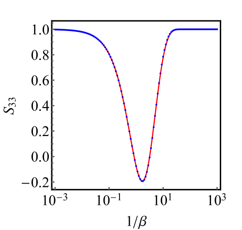
(b)

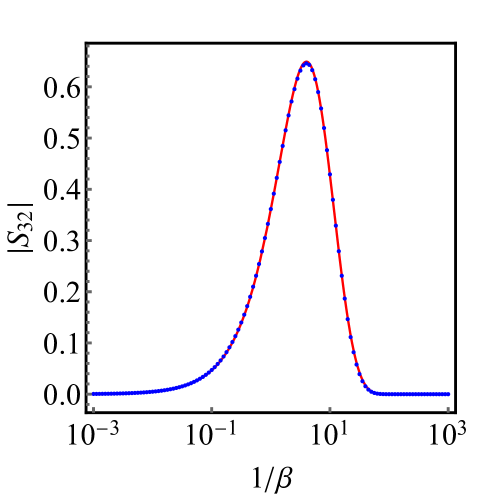
Figure 2: The numerically calculated $S_{33}$ and $|S_{32}|$ vs. $1/\beta$ and their fittings for evolution under the Hamiltonian (7) with its parameters given by Eqs. (57) and (58): (a) $S_{33}$ fitted by $(1-2e^{-0.219/\beta})(1-2e^{-0.827/\beta})$ and (b) $|S_{32}|$ fitted by $1.29e^{-0.108/\beta}(1-e^{-0.373/\beta})$. The dots are from numerics, and the solid curves are the fittings.

V Application to a $5$-site SSH chain

In this section, we are going to show that the choice of the set of parameters in (57) and (58) physically corresponds to a $5$-site SSH chain which couplings change linearly in time.

V.1 Odd-sized SSH chain under a linear quench

We will first consider a general odd-sized SSH chain with $2N-1$ sites with zero onsite energies, whose Hamiltonian reads:

$$H_{SSH}=\left(\begin{array}[]{ccccccc}0&J_{1}&0&0&\cdots&0&0\\ J_{1}&0&J_{2}&0&\cdots&0&0\\ 0&J_{2}&0&J_{1}&\cdots&0&0\\ 0&0&J_{1}&0&\cdots&0&0\\ \vdots&\vdots&\vdots&\vdots&\ddots&\vdots&\vdots\\ 0&0&0&0&\cdots&0&J_{2}\\ 0&0&0&0&\cdots&J_{2}&0\end{array}\right).$$ (70)

We take the couplings to change linearly in time as:

$$J_{1}=\frac{1}{2}+\beta t,\quad J_{2}=\frac{1}{2}-\beta t.$$ (71)

We will call it a linear quench. At $t=0$ the two couplings equal, and at $t=\pm 1/(2\beta)$ the chain is fully dimerized.

Since the Hamiltonian (70) depends linearly on time, it belongs to the multistate LZ model. We will transform it to the so-called diabatic basis which is the standard form of a multistate LZ model, which has its time-dependent part resting only on the diagonal elements. For this purpose, we first rewrite (70) as

$$H_{SSH}=Bt+A,$$ (72)

where

$$B=\beta\left(\begin{array}[]{ccccccc}0&1&0&0&\cdots&0&0\\ 1&0&-1&0&\cdots&0&0\\ 0&-1&0&1&\cdots&0&0\\ 0&0&1&0&\cdots&0&0\\ \vdots&\vdots&\vdots&\vdots&\ddots&\vdots&\vdots\\ 0&0&0&0&\cdots&0&-1\\ 0&0&0&0&\cdots&-1&0\end{array}\right),$$ (80)

and

$$A=\frac{1}{2}\left(\begin{array}[]{ccccccc}0&1&0&0&\cdots&0&0\\ 1&0&1&0&\cdots&0&0\\ 0&1&0&1&\cdots&0&0\\ 0&0&1&0&\cdots&0&0\\ \vdots&\vdots&\vdots&\vdots&\ddots&\vdots&\vdots\\ 0&0&0&0&\cdots&0&1\\ 0&0&0&0&\cdots&1&0\end{array}\right).$$ (88)

A transformation to the diabatic basis is then realized by a unitary transformation to diagonalize of the matrix $B$. The eigenvalues of $B$ read:

$$\epsilon_{j}=2\sin\frac{k_{j}}{2},$$ (89)

where $k_{j}=\pi j/N$ with $j=-N+1,\ldots,0,\ldots,N-1$. The corresponding eigenstates are:

$$\psi_{j}=(\psi_{1,j},\psi_{2,j},\ldots,\psi_{2N-1,j})^{T},$$ (90)

$$\psi_{x,j}=\frac{1}{\sqrt{N}}\sin(\frac{1}{2}k_{j}x),\quad\textrm{for }x\textrm{ even,}$$

$$\psi_{x,j}=\frac{1}{\sqrt{N}}\cos(\frac{1}{2}k_{j}x),\quad\textrm{for }x\textrm{ odd,}$$

where $x=1,2,\ldots,2N-1$ labels the sites. A unitary transformation with the matrix $V=(\psi_{1},\psi_{2},\ldots,\psi_{2N-1})$ then transforms $H$ to the diabatic basis, which we denote as $H_{LZ}$:

$$H_{LZ}=V^{T}H_{SSH}V=V^{T}BVt+V^{T}AV$$

$$\equiv B_{LZ}t+A_{LZ}.$$ (91)

Since all elements of the matrix $V$ are real, this transformation is also orthogonal. The matrix $B_{LZ}$ is, by construction, a diagonal matrix made of the eigenvalues:

$$(B_{LZ})_{l,l}=2\beta\sin(\frac{1}{2}k_{l}),$$ (92)

where $l=-N+1,\ldots,N-1$ (for convenience, we labelled the rows and columns of the matrix $B_{LZ}$ from $-N+1$ to $N-1$ instead of from $1$ to $2N-1$). The elements of the matrix $A_{LZ}$ can also be obtained in closed forms – evaluation of $V^{T}AV$ show that they can be written as imaginary parts of sums of certain geometric sequences, performing which leads to the result

$$(A_{LZ})_{l,m}=\frac{1}{N}\frac{\cos\frac{k_{l}}{2}\cos\frac{k_{m}}{2}}{\sin\frac{k_{l}}{2}+\sin\frac{k_{m}}{2}},\quad\textrm{for odd $m+l$},$$

$$(A_{LZ})_{l,m}=0,\quad\textrm{otherwise},$$ (93)

where $l=-N+1,\ldots,N-1$ and $m=-N+1,\ldots,N-1$.

The Hamiltonian $H_{LZ}=B_{LZ}t+A_{LZ}$ is now of the standard form of an multistate LZ model, from which we can read out several of its properties. First, since $A_{LZ}$’s diagonal elements are zero, the diabatic energy levels all cross at the same point. Second, the states are separated into two groups: one group for states with even indices and the other group for states with odd indices, and the coupling between any two states within the same group is zero. It thus belongs to the class of bipartite models studied in cross-2017 . Finally, as a result of the chiral symmetry of the original SSH model, the adiabatic energy diagram of $H_{LZ}$ is symmetric under a reflection of $E\rightarrow-E$, and there is a state with permanent zero energy – the state with index $0$.

Regardless of the above properties, the general model (V.1) at an arbitrary $N$ is very complicated, and it is not obvious at all if it is exactly solvable. But for a small $N$ the model is simple enough, and there is a hope to solve it. At $N=2$, the model can be recognized as a $3$-state bow-tie model bow-tie , which is indeed integrable and exactly solvable. At $N=3$, the Hamiltonian is a $5\times 5$ matrix. Calculating out the matrix elements using the above expressions of $(B_{LZ})_{l,l}$ and $(A_{LZ})_{l,m}$, one finds that this Hamiltonian is just the previously discussed Hamiltonian (7) with its parameters given by Eqs. (57) and (58), if the levels labelled by $-2,-1,0,1,2$ in (V.1) are identified as levels $2,1,3,5,4$ in (7), respectively. Thus, our result of the solution of the model (1) can be applied in studying a $5$-site SSH chain under a linear quench, which we discuss in the next subsection.

V.2 $5$-site SSH chain under a linear quench

The Hamiltonian of a $5$-site SSH chain under a linear quench reads:

$$H_{5,SSH}=\left(\begin{array}[]{ccccc}0&J_{1}&0&0&0\\ J_{1}&0&J_{2}&0&0\\ 0&J_{2}&0&J_{1}&0\\ 0&0&J_{1}&0&J_{2}\\ 0&0&0&J_{2}&0\end{array}\right).$$ (99)

where $J_{1}=\frac{1}{2}+\beta t$ and $J_{2}=\frac{1}{2}-\beta t$ as before. An illustration of this model is shown in Fig. 3(a). Its adiabatic energy diagram, Fig. 3(b), contains a state with permanent zero energy – the topological edge state. Especially, at two special times $t=\pm 1/(2\beta)$ the couplings take $J_{1}=0$ or $J_{2}=0$, respectively, i.e. the chain splits into isolate dimers and an isolate site at the left/right end. A quench from $t=-1/(2\beta)$ to $t=1/(2\beta)$ connects the two dimerized limits, as illustrated in Fig. 3(c).

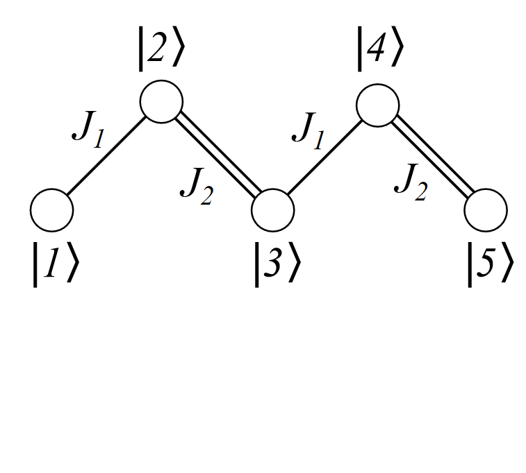
(a) (b)

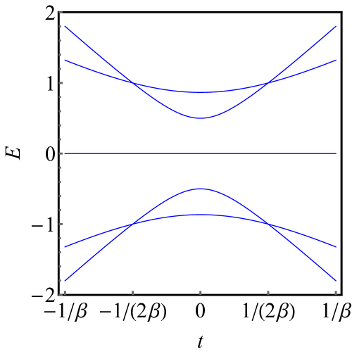
(c)

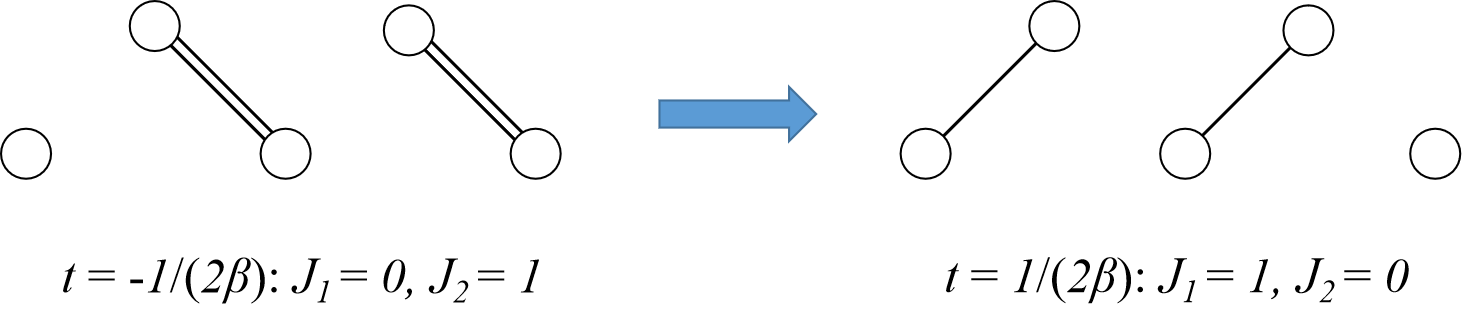
Figure 3: A 5-state SSH chain under a linear quench: (a) a sketch of the chain with $5$ sites; (b) the adiabatic energy diagram $E$ vs. $t$; (c) The chain under a quench from $t=-1/(2\beta)$ to $t=1/(2\beta)$ that connects the two dimerized limits.

As discussed in the last subsection, the Hamiltonian (99) is connected to the Hamiltonian (7) with parameters (57) and (58) by an orthogonal transformation:

$$H_{5,LZ}=V^{T}H_{5,SSH}V.$$ (100)

The evolution operator of the SSH chain $U_{5,SSH}(t_{f},t_{i})$ is then related to that of the LZ model by the same transformation:

$$U_{5,SSH}(t_{f},t_{i})={\cal T}e^{-i\int_{t_{i}}^{t_{f}}H_{5,SSH}dt}$$

$$={\cal T}e^{-i\int_{t_{i}}^{t_{f}}VH_{5,LZ}V^{T}dt}=V{\cal T}e^{-i\int_{t_{i}}^{t_{f}}H_{5,LZ}dt}V^{T}$$

$$=VU_{5,LZ}(t_{f},t_{i})V^{T}.$$ (101)

For this $5$-site chain we have $N=3$, and the explicit form of the matrix $V$ is:

$$V=\left(\begin{array}[]{ccccc}\frac{1}{2\sqrt{3}}&\frac{1}{2}&\frac{1}{\sqrt{3}}&\frac{1}{2}&\frac{1}{2\sqrt{3}}\\ -\frac{1}{2}&-\frac{1}{2}&0&\frac{1}{2}&\frac{1}{2}\\ -\frac{1}{\sqrt{3}}&0&\frac{1}{\sqrt{3}}&0&-\frac{1}{\sqrt{3}}\\ \frac{1}{2}&-\frac{1}{2}&0&\frac{1}{2}&-\frac{1}{2}\\ \frac{1}{2\sqrt{3}}&-\frac{1}{2}&\frac{1}{\sqrt{3}}&-\frac{1}{2}&\frac{1}{2\sqrt{3}}\\ \end{array}\right).$$ (107)

Thus, we can express any scattering amplitude of the $5$-site SSH chain in terms of those of the LZ model (7). For an evolution from $t=-T$ to $t=T$ with a large $T$, the results in the previous two sections can then be used.

One may also be interested in a quench from $t=-1/(2\beta)$ to $t=1/(2\beta)$, as sketched in Fig. 3(c). Especially, let’s take the system to be initially localized at the left edge $|1\rangle$ and ask how this state will transfer under such a quench. In Fig. 4 we plot the scattering amplitudes $S_{1\rightarrow 1}$ and $S_{1\rightarrow 5}$ for this quench (both amplitudes turn out to be always real – a result of symmetries). $S_{1\rightarrow 1}$ corresponds to the probability that the state stays on the left end, and $S_{1\rightarrow 5}$ the probability that the state transfers to the right end. We see that as $\beta$ decreases, $S_{1\rightarrow 1}$ decreases from $1$ to $0$ after some oscillations, whereas $S_{1\rightarrow 5}$ increases from $0$ to $1$. These tendencies are expected, since at large $\beta$ the state does not have time to transfer so $S_{1\rightarrow 1}$ is close to $1$, whereas at small $\beta$ the evolution is adiabatic so $S_{1\rightarrow 5}$ is close to $1$. Besides, we see that the amplitude $S_{1\rightarrow 5}$ becomes close to the previously calculated $S_{33}$ (for a $t=-\infty$ to $t=\infty$ evolution of the model (7) with parameters (57) and (58)) at around $\beta<0.1$. Actually $S_{33}$ can be interpreted as the amplitude of adiabatic evolution to stay on the zero energy eigenstate; the left or right edge states at $t=\pm 1/(2\beta)$ are both instantaneous eigenstates along this adiabatic evolution. For $\beta$ small enough, the LZ transition happens well within the time interval from $t=-1/(2\beta)$ to $t=1/(2\beta)$, so the scattering amplitude $S_{1\rightarrow 5}$ can be approximated by $S_{33}$ from a $t=-\infty$ to $t=\infty$ evolution.

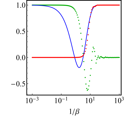
Figure 4: The numerically calculated $S_{1\rightarrow 1}$ (green dots) and $S_{1\rightarrow 5}$ (red dots) vs. $1/\beta$ for a $5$-site SSH chain (99) under a linear quench from $t=1/(2\beta)$ to $t=1/(2\beta)$. For comparison, the blue curve is $S_{33}$ for a $t=-\infty$ to $t=\infty$ evolution of the model (7) with parameters (57) and (58).

VI Conclusions and Discussions

We study a $5$-state LZ model for which integrability is not helpful in finding its solutions. We analyze the constraints on its scattering matrix and show that the transition probabilities depend on two independent unknowns. For a particular choice of parameters, by fitting to exact results from numerical simulations of the Schrödinger equation we find that these two independent unknowns can be approximately expressed by analytical expressions. Thus, we obtain nearly exact solution of all transition probabilities of this model. We also show that this model can describe a $5$-site SSH chain under a linear quench of its couplings.

We expect that our method could also be used to solve other multistate LZ models not necessarily integrable and when analytical constraints on their scattering matrices are insufficient for their solutions. For example, one could just consider the same Hamiltonian (1) but with a different choice of couplings. Then all the previous constraints apply and again one need to find two independent unknowns by fitting. One could also consider a completely different model; we expect that the method generally works better for a model when the number of independent unknowns is small after using all constraints on its scattering matrix. Thus, it would be interesting to look at other currently unsolved multistate LZ models with small numbers of levels and with symmetries as rich as possible.

Another interesting possibility is to perform a fitting with the help of computers, especially artificial intelligence. The fitting problem we face here is basically to find an unknown symbolic expression to describe a set of data. Such kind of problem is known in computer science as symbolic regression, which is a rapidly growing research area Udrescu-2020 ; La-Cava-2021 . In our case, the data set is generated from exact numerical solution of an equation (the Schrödinger equation of the $5$-state LZ model) at different choices of parameters. This is exactly the type of problems studied in a recent work Ashhab-2023 , where a state-of-the-art symbolic regression package based on machine learning was tested on looking for symbolic solutions of the LZ model and a few multistate LZ models. Although these tests show that still the package’s performance seems not better than human brains’, it is possible that in the future artificial intelligence will outperform human in such fitting works, and thus it will become a powerful tool in studying problems like the one considered in this paper.

Appendix A: Simplification of constraints on the scattering matrix

In this appendix, we present details of simplification of the constraints on the elements of the scattering matrix $S$, namely, Eqs. (18)-(40).

We first demonstrate that, although there are originally $6$ complex unknowns, the system of equations depends on only $4$ phases. There are $8$ equations that involve phases: the last two HCs (35) and (40), and the last $6$ unitarity constraints (22)-(27). In terms of the $4$ rotated elements defined in (45)-(48), the $6$ unitarity constraints involving phases read:

$$2S_{11}\tilde{S}_{51}+2\tilde{S}_{21}\tilde{S}_{41}+|S_{31}|^{2}=0,$$ (A1)

$$2\tilde{S}_{21}^{*}\tilde{S}_{41}+2S_{22}\tilde{S}_{42}+|S_{32}|^{2}=0,$$ (A2)

$$(S_{22}-S_{11})\tilde{S}_{21}+|S_{31}S_{32}|+\tilde{S}_{41}\tilde{S}_{42}^{*}-\tilde{S}_{51}\tilde{S}_{41}^{*}=0,$$ (A3)

$$(S_{33}-S_{11})|S_{31}|+\tilde{S}_{21}|S_{32}|+\tilde{S}_{41}|S_{32}|-\tilde{S}_{51}|S_{31}|=0,$$ (A4)

$$(S_{22}-S_{11})\tilde{S}_{41}+\tilde{S}_{21}\tilde{S}_{42}+|S_{31}S_{32}|-\tilde{S}_{51}\tilde{S}_{21}^{*}=0,$$ (A5)

$$(S_{22}+S_{33})|S_{32}|+\tilde{S}_{21}^{*}|S_{31}|+\tilde{S}_{42}|S_{32}|+\tilde{S}_{41}|S_{31}|=0.$$ (A6)

We see the phases of $S_{31}$ and $S_{32}$ drop out from all these equations. This also happens in the $3$rd HC (35), which becomes:

$$YS_{33}-S_{11}|S_{32}|^{2}+S_{22}|S_{31}|^{2}-|S_{31}S_{32}|(\tilde{S}_{21}+\tilde{S}^{*}_{21})=Y.$$ (A7)

The $4$th HC (40) involves calculation of the determinant of a $4\times 4$ matrix. After some tedious algebra with repetitive usages of other constraints, we find that it reduces to a simple form

$$[(1+S_{11})^{2}-|S_{51}^{2}|](S_{11}-S_{22})$$

$$+|S_{31}|^{2}[1+S_{11}-\frac{1}{2}(\tilde{S}_{51}+\tilde{S}^{*}_{51})]=0.$$ (A8)

Therefore, the system of equations involves only $4$ complex unknowns, or equivalently, $4$ phases.

We next show that all $4$ rotated elements (or equivalently, their $4$ phases) can be determined up to a sign by the real elements and the magnitudes of complex elements. From (A1) and (A2), we get:

$$\tilde{S}_{51}=-\frac{1}{S_{11}}(\tilde{S}_{21}\tilde{S}_{41}+\frac{1}{2}|S_{31}|^{2}),$$ (A9)

$$\tilde{S}_{42}=-\frac{1}{S_{22}}(\tilde{S}_{21}^{*}\tilde{S}_{41}+\frac{1}{2}|S_{32}|^{2}).$$ (A10)

On the other hand, from (A4), we get:

$$\tilde{S}_{51}=S_{33}-S_{11}+(\tilde{S}_{21}+\tilde{S}_{41})\frac{|S_{32}|}{|S_{31}|}.$$ (A11)

From Eqs. (A9) and (A11), we can express $\tilde{S}_{41}$ in terms of $\tilde{S}_{21}$ as:

$$\tilde{S}_{41}=-\frac{S_{11}(S_{33}-S_{11})+\frac{1}{2}|S_{31}|^{2}+S_{11}\tilde{S}_{21}\frac{|S_{32}|}{|S_{31}|}}{\tilde{S}_{21}+S_{11}\frac{|S_{32}|}{|S_{31}|}}.$$ (A12)

Therefore, $\tilde{S}_{41}$, $\tilde{S}_{51}$, and $\tilde{S}_{42}$ can all be expressed in terms of the three real elements $S_{11}$, $S_{22}$ and $S_{33}$, the two magnitudes $|S_{31}|$ and $|S_{32}|$, and $\tilde{S}_{21}$. Besides, Eq. (A7) shows that $\tilde{S}_{21}+\tilde{S}_{21}^{*}$ can be expressed in terms of the three real elements and the two magnitudes. So if all the real elements and the magnitudes of complex elements are known, all the $4$ four unknown phases can be determined up to a sign. There is still a sign ambiguity when determining the phases of $\tilde{S}_{21}$. Actually, each the original $14$ constraints is invariant if we send the $4$ rotated elements to their complex conjugates. Thus, the sign of the phase of $\tilde{S}_{21}$ cannot be determined by the real elements and the magnitudes. This sign needs to be fixed by the solution of the actual evolution process.

Finally, we show that all the real elements and the magnitudes of complex elements can be expressed in terms of two of them. There are totally $9$ of them – $3$ real elements and $6$ magnitudes of complex elements. The original set of constraints already contain $6$ independent relations on them, namely, Eqs. (18)-(21) and Eqs. (28)-(31). From the constraints involving phases, we can derive one more constraint on the real elements and the magnitudes. Plugging Eq. (A12) into Eq. (A11), we express $\tilde{S}_{51}$ in terms of $\tilde{S}_{21}$ as:

$$\tilde{S}_{51}=\frac{1}{2}(S_{33}+1)-X\frac{X(1+S_{33})-|S_{32}|^{2}}{2Y}$$

$$+\frac{|S_{32}|}{|S_{31}|}\frac{X(1+S_{33})-|S_{32}|^{2}+2Y}{2Y}\tilde{S}_{21}.$$ (A13)

Calculating the real part of $\tilde{S}_{51}$ with the help of some constraints involving only real elements and magnitudes, we get:

$$\frac{1}{2}(\tilde{S}_{51}+\tilde{S}_{51}^{*})=\frac{1}{2}(S_{33}+1)+X$$

$$+\frac{S_{33}-1}{8Y|S_{31}|^{2}}[X(1+S_{33})-|S_{32}|^{2}+2Y]^{2}.$$ (A14)

Plugging this into (Appendix A: Simplification of constraints on the scattering matrix) and simplifying, we get an expression of $|S_{51}|^{2}$ in terms of $|S_{32}|$ and $S_{33}$ only:

$$|S_{51}|^{2}=\frac{1}{4}(1+S_{33})^{2}+|S_{32}|^{2}+X^{2}-Y-Z.$$ (A15)

This equation and the original $6$ constraints Eqs. (18)-(21) and Eqs. (28)-(31) form the set of constraints on the real elements and the magnitudes. We checked that there are no other independent relations on the real elements and the magnitudes. Thus, the total number of independent equations on the real elements and the magnitudes is $7$, and we will have $9-7=2$ independent real elements and magnitudes after these $7$ equations are used. If we choose the two independent unknowns to be $S_{33}$ and $|S_{32}|$, and the rest $7$ are then expressed as Eqs. (49)-(55) in the main text.

Summarizing, from the $14$ constraints (18)-(40) on the elements of the scattering matrix $S$, all unknowns can be determined in terms of two of them (e.g. $S_{33}$ and $|S_{32}|$), up to an overall sign of the phases of the complex unknowns.

References

- (1) L. Landau, Zur Theorie der Energieubertragung. II, Phys. Z. Sowj. 2, 46 (1932).
- (2) C. Zener. Non-Adiabatic Crossing of Energy Levels, Proc. R. Soc. 137, 696 (1932).
- (3) E. Majorana, Atomi orientati in campo magnetico variabile, Nuovo Cimento 9, 43 (1932).
- (4) E. C. G. Stückelberg. Theorie der unelastischen Stösse zwischen Atomen, Helv. Phys. Acta. 5, 370 (1932).
- (5) Yu. N. Demkov and V. I. Osherov, Zh. Eksp. Teor. Fiz. 53, 1589 (1967) [Stationary and nonstationary problems in quantum mechanics that can be solved by means of contour integration, Sov. Phys. JETP 26, 916 (1968)].
- (6) F. T. Hioe, -level quantum systems with dynamic symmetry, J. Opt. Soc. Am. B 4, 1327 (1987).
- (7) V. N. Ostrovsky and H. Nakamura, Exact analytical solution of the -level Landau-Zener-type bow-tie model, J. Phys. A: Math. Gen. 30, 6939 (1997).
- (8) Y. N. Demkov and V. N. Ostrovsky, Multipath interference in a multistate Landau-Zener-type model, Phys. Rev. A 61, 032705 (2000).
- (9) Y. N. Demkov and V. N. Ostrovsky, The exact solution of the multistate Landau-Zener type model: the generalized bow-tie model, J. Phys. B: At. Mol. Opt. Phys. 34, 2419 (2001).
- (10) N. A. Sinitsyn, Multiparticle Landau-Zener model: Application to quantum dots, Phys. Rev. B 66, 205303 (2002).
- (11) V. L. Pokrovsky and N. A. Sinitsyn, Landau-Zener transitions in a linear chain, Phys. Rev. B 65, 153105 (2002).
- (12) N. A. Sinitsyn, Solvable four-state Landau-Zener model of two interacting qubits with path interference, Phys. Rev. B 92, 205431 (2015).
- (13) N. A. Sinitsyn, Exact transition probabilities in a -state Landau-Zener system with path interference, J. Phys. A: Math. Theor. 48, 195305 (2015).
- (14) N. A. Sinitsyn and F. Li, Solvable multistate model of Landau-Zener transitions in cavity QED, Phys. Rev. A 93, 063859 (2016).
- (15) C. Sun and N. A. Sinitsyn, Landau-Zener extension of the Tavis-Cummings model: Structure of the solution, Phys. Rev. A 94, 033808 (2016).
- (16) N. A. Sinitsyn and V. Y. Chernyak, The quest for solvable multistate Landau-Zener models, J. Phys. A: Math. Theor. 50, 255203 (2017).
- (17) V. Y. Chernyak, N. A. Sinitsyn, and C. Sun. A large class of solvable multistate Landau-Zener models and quantum integrability, J. Phys. A: Math. Theor. 51, 245201 (2018).
- (18) A. Patra and E. A. Yuzbashyan, Quantum integrability in the multistate Landau-Zener problem, J. Phys. A: Math. Theor. 48, 245303 (2015).
- (19) N. A. Sinitsyn, E. A. Yuzbashyan, V. Y. Chernyak, A. Patra, and C. Sun, Integrable time-dependent quantum Hamiltonians, Phys. Rev. Lett. 120, 190402 (2018).
- (20) E. A. Yuzbashyan, Integrable time-dependent Hamiltonians, solvable Landau-Zener models and Gaudin magnets, Ann. Phys. 392, 323 (2018).
- (21) Dynamic spin localization and -magnets, V. Y. Chernyak, N. A. Sinitsyn, and C. Sun, Phys. Rev. B 100, 224304 (2019).
- (22) V. Y. Chernyak, N. A. Sinitsyn, and C. Sun, Multitime Landau-Zener model: classification of solvable Hamiltonians, J. Phys. A: Math. Theor. 53, 185203 (2020).
- (23) V. Y. Chernyak, F. Li, C. Sun, and N. A. Sinitsyn, Integrable multistate Landau-Zener models with parallel energy levels, J. Phys. A: Math. Theor. 53, 295201 (2020).
- (24) V. Y. Chernyak and N. A. Sinitsyn, Integrability in the multistate Landau-Zener model with time-quadratic commuting operators, J. Phys. A: Math. Theor. 54, 115204 (2021).
- (25) L. Wang and C. Sun, No-go rules for multitime Landau-Zener models, Eur. Phys. J. Plus 137, 1204 (2022).
- (26) S. Brundobler and V. Elser, S-matrix for generalized Landau-Zener problem, J. Phys. A: Math. Gen. 26, 1211 (1993).
- (27) N. A. Sinitsyn, Counterintuitive transitions in the multistate Landau-Zener problem with linear level crossings, J. Phys. A: Math. Gen. 37, 10691 (2004).
- (28) A. V. Shytov, Landau-Zener transitions in a multilevel system: An exact result, Phys. Rev. A 70, 052708 (2004).
- (29) N. A. Sinitsyn, J. Lin, and V. Y. Chernyak, Constraints on scattering amplitudes in multistate Landau-Zener theory, Phys. Rev. A 95, 012140 (2017).
- (30) F. Li, C. Sun, V. Y. Chernyak, and N. A. Sinitsyn, Multistate Landau-Zener models with all levels crossing at one point, Phys. Rev. A 96, 022107 (2017).
- (31) N. A. Sinitsyn, Exact results for models of multichannel quantum nonadiabatic transitions, Phys. Rev. A 90, 062509 (2014).
- (32) S. M. Udrescu and M. Tegmark, AI Feynman: A physics-inspired method for symbolic regression, Sci. Adv. 6, 2631 (2020).
- (33) W. La Cava, P. Orzechowski, B. Burlacu, F. O. de Franca, M. Virgolin, Y. Jin, M. Kommenda, and J. H. Moore, Contemporary Symbolic Regression Methods and their Relative Performance, arXiv:2107.14351 [cs.NE] 29 Jul 2021.
- (34) S. Ashhab, Using machine learning to find exact analytic solutions to analytically posed physics problems, arXiv:2306.02528 [physics.comp-ph] 5 Jun 2023.