SSCBench: Monocular 3D Semantic Scene
Completion Benchmark in Street Views

Yiming Li^1,∗, Sihang Li^1,∗, Xinhao Liu^1,∗, Moonjun Gong^1,, Kenan Li¹, Nuo Chen¹,
Zijun Wang¹, Zhiheng Li¹, Tao Jiang², Fisher Yu³, Yue Wang⁴, Hang Zhao²,
Zhiding Yu⁴, Chen Feng^1,
¹New York University, ²Tsinghua University, ³ETH Zurich, ⁴NVIDIA Equal contributionThe corresponding author is Chen Feng cfeng@nyu.edu

Abstract

Monocular scene understanding is a foundational component of autonomous systems. Within the spectrum of monocular perception topics, one crucial and useful task for holistic 3D scene understanding is semantic scene completion (SSC), which jointly completes semantic information and geometric details from RGB input. However, progress in SSC, particularly in large-scale street views, is hindered by the scarcity of high-quality datasets. To address this issue, we introduce SSCBench, a comprehensive benchmark that integrates scenes from widely used automotive datasets (e.g., KITTI-360, nuScenes, and Waymo). SSCBench follows an established setup and format in the community, facilitating the easy exploration of SSC methods in various street views. We benchmark models using monocular, trinocular, and point cloud input to assess the performance gap resulting from sensor coverage and modality. Moreover, we have unified semantic labels across diverse datasets to simplify cross-domain generalization testing. We commit to including more datasets and SSC models to drive further advancements in this field.

1 Introduction

Understanding 3D scenes from a single RGB image is crucial and meaningful in vision and robotics, with monocular perception tasks like object detection (Wang et al., 2022), tracking (Hu et al., 2022), and depth estimation (Yuan et al., 2022) garnering significant attention. The emerging field of 3D semantic scene completion (SSC) (Roldao et al., 2022) seeks to jointly infer complete 3D semantics and geometry from a sparse and partial observation (e.g., an RGB image). The resulting volumetric representation seamlessly integrates occupancy and semantic information, facilitating robotic scene understanding and planning capabilities in street views.

One critical challenge in SSC is to generate accurate ground truth labels, especially in street views. Given the current limitations of 3D sensing technology, achieving a perfectly comprehensive 3D representation is impossible. The pioneering SemanticKITTI benchmark (Behley et al., 2019) proposes to leverage the temporal information through the aggregation of different LiDAR sweeps, which can effectively reveal previously occluded 3D surfaces. Meanwhile, it excludes 3D voxels not observed from all viewpoints during driving. Consequently, SemanticKITTI provides relatively comprehensive and accurate ground truth labels for SSC tasks.

While SemanticKITTI is a valuable resource for learning sparse-to-dense mapping, its limited scale and diversity impede the development of more powerful and generalizable SSC models. Another significant limitation of SemanticKITTI is the omission of dynamic objects during ground truth generation, resulting in inaccurate labels. Hence, there is an urgent need for a large-scale SSC dataset with reliable ground truth to advance learning-based scene understanding in street views.

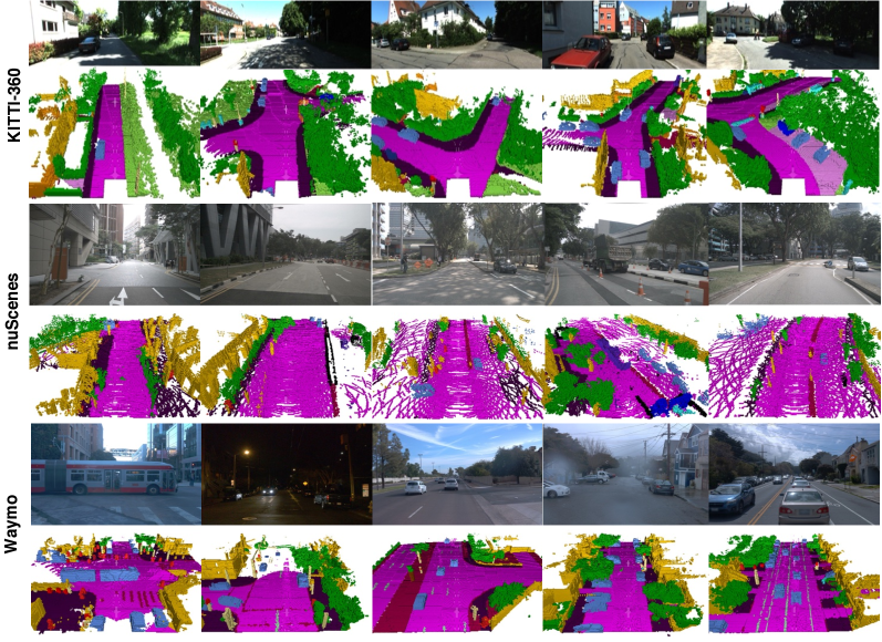
To this end, we introduce SSCBench, a large-scale benchmark comprising diverse street views sourced from well-established automotive datasets, including KITTI-360 (Liao et al., 2022), nuScenes (Caesar et al., 2020), and Waymo (Sun et al., 2020), as illustrated in Fig. 1. To enhance label accuracy, we utilize the 3D bounding box labels provided in these datasets to synchronize measurements of dynamic objects. Our key features include (a) accessibility: we provide datasets in a format compatible with SemanticKITTI, facilitating seamless usage within the community; (b) large scale: we offer an extensive dataset with $\sim$ 8 times more frames than SemanticKITTI, encompassing diverse geographic locations across six cities; (c) comprehensiveness: we mainly focus on SSC methods with monocular input. Additionally, we utilize trinocular input to compare the single-view and panoramic-view methods and use point cloud input to show the gap between camera-based and LiDAR-based methods. Furthermore, we have unified semantic labels across different datasets in SSCBench, facilitating cross-domain generalization experiments. We plan to continually incorporate novel automotive datasets and SSC algorithms to drive further advancements in the field.

Refer to caption — Figure 1: Visualizations of SSCBench derived from KITTI-360 (Liao et al., 2022), nuScenes (Caesar et al., 2020), and Waymo (Sun et al., 2020). We showcase accurate SSC ground truth in a variety of street views. We commit to incorporating novel datasets for further development.

2 Related Works

Monocular Perception and 3D Semantic Scene Completion. The simplicity, efficiency, affordability, and accessibility of monocular cameras have made monocular perception a focal point of attention in the vision and robotics community. This has resulted in extensive research into various tasks, including depth estimation (Dong et al., 2022), 3D object detection and tracking (Enzweiler & Gavrila, 2008), as well as localization and mapping (Younes et al., 2017). Song et al. (2017) introduce the concept of monocular 3D semantic scene completion (SSC), which seeks to reconstruct and complete the semantics as well as geometry within a 3D volume from a single depth image. However, they only consider the bounded indoor scenarios due to the lack of outdoor datasets. Behley et al. (2019) build the first outdoor dataset based on KITTI (Geiger et al., 2012) for 3D semantic scene completion in street views. Existing approaches usually depend on 3D inputs, such as LiDAR point clouds (Roldao et al., 2020; Cheng et al., 2021a; Rist et al., 2021; Yan et al., 2021), while recent monocular vision-based solutions also emerge (Cao & de Charette, 2022; Li et al., 2023). However, the development of outdoor SSC is hindered by the lack of datasets, with SemanticKITTI (Behley et al., 2019) being the only dataset supporting SSC in street views. Building diverse datasets is imperative to unlock the full potential of SSC for autonomous systems.

Point Cloud Segmentation in Street Views. 3D LiDAR segmentation aims to assign point-wise semantic labels for point clouds, including a range of specific tasks, like LiDAR semantic (Hu et al., 2020; Qiu et al., 2021; Milioto et al., 2019; Xu et al., 2020; Cortinhal et al., 2020), panoptic (Zhou et al., 2021; Hong et al., 2021; Behley et al., 2021), and 4D panoptic segmentation (Kreuzberg et al., 2022; Aygun et al., 2021). In this field, point-based methods, stemming from PointNet++ (Qi et al., 2017), perform well on small synthetic point cloud (Yi et al., 2016) rather than sparse LiDAR point cloud, with sampling and gathering disordered neighbors. Voxel-based approaches (Zhu et al., 2021; Tang et al., 2020; Li et al., 2022a; Cheng et al., 2021b) process point clouds by initially partitioning 3D space into voxels through Cartesian coordinates. Note that 3D LiDAR segmentation aims to classify and understand the scenes based on raw LiDAR scans, while 3D semantic scene completion includes the completion of occluded areas, with input of camera or LiDAR.

Table 1: Overview of widely-used autonomous driving datasets with multimodal sensors. C denotes camera and L denotes LiDAR. Most datasets provide bounding annotations for 3D detection, yet only a few of them provide semantic labels for the LiDAR point cloud due to the high cost. Note that ApolloScape (Huang et al., 2019) only provides 3D semantic labels for the static environments.

Datasets	Year	Sensors	Annotations	# Fr. with Pts Ann.	Sequential
KITTI Geiger et al. (2012)	CVPR 2012	C&L	3D Bbox	N.A.	✗
SemanticKITTI Behley et al. (2019)	ICCV 2019	C&L	3D Pts.	20K	✓
nuScenes Caesar et al. (2020)	CVPR 2019	C&L	3D Bbox	N.A.	✓
Panoptic nuScenes Fong et al. (2022)	RA-L 2022	C&L	3D Pts.	40K	✓
Waymo Sun et al. (2020)	CVPR 2020	C&L	3D Bbox&Pts.	230K	✓
KITTI-360 Liao et al. (2022)	T-PAMI 2022	C&L	3D Bbox&Pts.	100K	✓
ApolloScape Huang et al. (2019)	T-PAMI 2019	C&L	3D Bbox&Pts.	N.A.	✓
Argoverse Chang et al. (2019)	CVPR 2019	C&L	3D Bbox	N.A.	✓
ONCE Mao et al.	NeurIPS 2021	C&L	3D Bbox	N.A.	✓
Lyft Level 5 Kesten et al. (2019)	2019	C&L	3D Bbox	N.A.	✓
A*3D Pham et al. (2020)	ICRA 2020	C&L	3D Bbox	N.A.	✓
A2D2 Geyer et al. (2020)	2020	C&L	3D Bbox	N.A.	✗

Autonomous Driving Dataset and Benchmark. Autonomous driving research thrives on high-quality datasets, which serve as the lifeblood for training and evaluating perception (Caesar et al., 2020), prediction (Ettinger et al., 2021), and planning algorithms (Hu et al., 2023). In 2012, the pioneering KITTI dataset sparked a revolution in autonomous driving research, unlocking a multitude of tasks including object detection, tracking, mapping, and optical/depth estimation (Geiger et al., 2012; 2013; Fritsch et al., 2013; Menze & Geiger, 2015; Chen et al., 2023). Since then, the research community has embraced the challenge, giving rise to a wealth of datasets. These datasets push the boundaries of autonomous driving research by addressing challenges posed by multimodal fusion (Caesar et al., 2020), multi-tasking learning (Huang et al., 2018; Liao et al., 2022), adverse weather (Pitropov et al., 2021), collaborative driving (Agarwal et al., 2020; Li et al., 2022b; Xu et al., 2023), repeated driving (Diaz-Ruiz et al., 2022), and dense traffic scenarios (Pham et al., 2020; Xiao et al., 2021), etc. There are several impactful and widely-used driving datasets such as KITTI-360 (Liao et al., 2022), nuScenes (Caesar et al., 2020), and Waymo (Sun et al., 2020). They provide LiDAR and camera recordings as well as point cloud semantics and bounding annotations, as summarized in Tab. 1. Therefore, we can create accurate ground truth labels for SSC by aggregating multiple semantic point clouds and leveraging the 3D boxes to handle dynamic objects.

Occ3D and OpenOccupancy. We compare SSCBench with the concurrent relevant work Occ3D (Tian et al., 2023). The differences lie in: (a) setup: Occ3D uses surrounding-view images as input, and only considers the reconstruction of 3D voxels visible to the camera. SSCBench considers a more challenging yet meaningful setup (also a well-established one): how to reconstruct and complete 3D semantics in both visible and occluded areas only with monocular visual input. This task requires reasoning about temporal information and 3D geometric relationships to get rid of the limited field of view; (b) scale: SSCBench provides more datasets than Occ3D and plans to add more due to the abundance of monocular driving recordings; (c) accessibility: we inherit the widely-used setup from the pioneer KITTI, thus making SSCBench more accessible to the community; (d) comprehensiveness: we benchmark SSC methods with monocular, trinocular, and point cloud input and provide unified labels for cross-domain generalization tests. Another relevant benchmark, OpenOccupancy (Wang et al., 2023), exhibits similar differences, notably its exclusive use of the nuScenes dataset (Caesar et al., 2020), which results in a limitation of diversity.

3 Dataset Curation

3.1 Revisit of SemanticKITTI

SemanticKITTI (Behley et al., 2019) extends the odometry dataset of the KITTI vision benchmark (Geiger et al., 2012) by providing point-wise semantic annotations for 22 driving sequences in Karlsruhe, Germany. SemanticKITTI not only supports 3D semantic segmentation but also serves as the first outdoor SSC benchmark. Similar to indoor SSC (Song et al., 2017), SemanticKITTI uses voxelized 3D representation widely employed in robotics such as occupancy grid mapping (Thrun, 2002). SemanticKITTI generates ground truth labels through voxelization of a dense semantic point cloud given by rigid registration of multiple LiDAR scans.

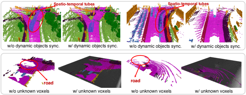
SemanticKITTI has two limitations. First, rigid registration with sensor poses can only handle measurements for static environments, resulting in traces produced by dynamic objects such as moving cars as shown in Fig. 2, which can confuse the 3D representation learning (Rist et al., 2021). Secondly, it is constrained by the limited scale and lack of diverse geographical coverage. The data collection is confined to a single city, resulting in training, validation, and test sets composed of 3,834, 815, and 3,992 frames, respectively, amounting to a total of 8,641 frames. However, this falls short of the large-scale benchmark necessary for comprehensive evaluation and generalization in the field.

3.2 SSCBench

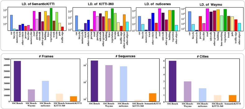
We aim to establish a large-scale SSC benchmark in street views that facilitates the training of robust and generalizable SSC models. To achieve this, we harness well-established and widely-used datasets and integrate them into a unified setup and format. Overall, our SSCBench, consisting of three subsets, includes 38,562 frames for training, 15,798 frames for validation, and 12,553 frames for testing respectively, amounting totally to 66,913 frames ( $\sim$ 67K), which greatly exceeds the scale of SemanticKITTI mentioned above by $\sim$ 7.7 times. In the following, we introduce three carefully designed datasets, all based on existing data sources, that collectively contribute to our SSCBench.

SSCBench-KITTI-360. KITTI-360 (Liao et al., 2022) represents a significant advancement in autonomous driving research, building upon the renowned KITTI dataset (Geiger et al., 2012). It introduces an enriched data collection framework with diverse sensor modalities as well as panoramic viewpoints (a perspective stereo camera plus a pair of fisheye cameras) and provides comprehensive annotations including consistent 2D and 3D semantic instance labels as well as 3D bounding primitives. The dense and coherent labels not only support established tasks such as segmentation and detection but also enable novel applications like semantic SLAM (Bowman et al., 2017) and novel view synthesis (Zhang et al., 2023a). While KITTI-360 includes point cloud-based semantic scene completion, the prevalent methodology for SSC remains centered around voxelized representations (Roldao et al., 2022), which exhibit broader applicability in robotics.

Remark. KITTI-360 covers a driving distance of 73.7km, comprising 300K images and 80K laser scans. While adhering to KITTI’s forward-facing camera setup, it offers greater geographical diversity and demonstrates minimal trajectory overlap with KITTI. Leveraging the open-source training and validation set, we build SSCBench-KITTI-360 consisting of 9 long sequences. To reduce redundancy, we sample every 5 frames following the SemanticKITTI SSC benchmark. The training set includes 8,487 frames from scenes 00, 02-05, 07, and 10, while the validation set comprises 1,812 frames from scene 06. The testing set comprises 2,566 frames from scene 09. In total, the dataset contains 12,865 ( $\sim$ 13K) frames, surpassing the scale of SemanticKITTI by $\sim$ 1.5 times.

SSCBench-nuScenes. Unlike KITTI’s forward-facing camera setup, nuScenes (Caesar et al., 2020) captures a complete 360-degree view around the ego vehicle. It provides a diverse range of multimodal sensory data, including camera images, LiDAR point clouds, and radar data, gathered in Boston and Singapore. nuScenes offers meticulous annotations for complex urban driving scenarios, including diverse weather conditions, construction zones, and varying illumination. Later on, panoptic nuScenes (Fong et al., 2022) extends the original nuScenes dataset with semantic and instance labels. With comprehensive metrics and evaluation protocols, nuScenes is widely employed in autonomous driving research (Gu et al., 2023; Hu et al., 2023; Li et al., 2021; Huang et al., 2023).

Remark. The nuScenes dataset consists of 1K 20-second scenes with labels provided only for the training and validation set, totaling 850 scenes. From the available 850 scenes, we allocate 500 scenes for training, 200 scenes for validation, and 150 scenes for testing. This distribution results in 20,064 frames for training, 8,050 frames for validation, and 5,949 frames for testing, totaling 34,078 frames ( $\sim$ 34K). This scale is approximately four times that of SemanticKITTI. As nuScenes only provides annotations for keyframes at a frequency of 2Hz, there is no downsampling in SSCBench-nuScenes.

SSCBench-Waymo. The Waymo dataset (Sun et al., 2020), collected from various locations in the US, offers a large-scale collection of multimodal sensor recordings. Waymo provides 5 cameras with a combined horizontal field of view of $\sim$ 230 degrees, slightly smaller than nuScenes. The data is captured in diverse conditions across multiple cities, including San Francisco, Phoenix, and Mountain View, ensuring broad geographical coverage within each city. It consists of 1000 scenes for training and validation, as well as 150 scenes for testing, with each scene spanning 20 seconds.

Remark. To construct SSCBench-Waymo, we utilize the open-source training and validation scenes and redistribute them into sets of 500, 298, and 202 scenes for training, validation, and testing, respectively. In order to reduce redundancy and training time for our benchmark, we downsample the original data by a factor of 10. This downsampling results in a training set of 10,011 frames, a validation set of 5,936 frames, and a test set of 4,038 frames, totaling 19,985 frames ( $\sim$ 20K).

3.3 Construction Pipeline

Prerequisites. To establish SSCBench, a driving dataset with multimodal recordings is required for LiDAR-based or camera-based SSC. The dataset should include sequentially collected 3D LiDAR point clouds with accurate sensor poses for geometry completion, per-point semantic annotations for semantic scene understanding, and 3D bounding annotations to handle dynamic instances.

Aggregation of Point Clouds. To generate a complete representation, our approach involves superimposing an extensive set of laser scans within a defined region in front of the vehicle. In short sequences like nuScenes and Waymo, we utilize future scans with measurements from the corresponding region to create a dense semantic point cloud. In long sequences like KITTI-360, which feature multiple loop closures, we incorporate all spatial neighboring point clouds in addition to the temporal neighborhood. Accurate sensor poses, provided by advanced SLAM systems (Bailey & Durrant-Whyte, 2006), greatly facilitate the aggregation of point clouds for the static environment. As for dynamic objects, we avoid the spatial-temporal tubes by synchronization. We utilize the instance label to transform dynamic objects to their spatial alignment within the current frame. As shown in Fig. 2, the spatial-temporal tubes are removed and the objects have a denser shape.

Voxelization of Aggregated Point Clouds. Voxelization is to discretize a continuous 3D space into a regular grid structure composed of volumetric elements called voxels, enabling the conversion of unstructured data into a structured format that can be efficiently processed by convolutional neural networks (CNNs) or vision transformers (ViTs). Voxelization introduces a trade-off between spatial resolution and memory consumption and offers a flexible and scalable representation for 3D perception (Maturana & Scherer, 2015; Zhou & Tuzel, 2018; Li et al., 2023). For easy integration, SSCBench adheres to SemanticKITTI’s setup, with a volume extending 51.2m ahead, 25.6m on each side, and 6.4m in height. Voxel resolution is 0.2m, resulting in a 256 $\times$ 256 $\times$ 32 voxel volume. Labels for each voxel are determined by majority voting among labeled points within it, while empty voxels are marked accordingly if no points are present.

Exclusion of Unknown Voxels. Capturing complete 3D outdoor dynamic scenes is nearly impossible without ubiquitous scene sensing. While it is possible to utilize spatial or prior knowledge-based inference, our intention is to ensure the fidelity of ground truth by minimizing errors originating from these steps. Hence, we only consider visible and probed voxels from all viewpoints during training and evaluation. Specifically, we first employ ray tracing from different perspectives to identify and remove occluded voxels within objects or behind walls. Furthermore, in datasets with sparse sensing, where numerous voxels remain unprobed, we remove these unknown voxels during training and evaluation to enhance the reliability of the ground truth labels as shown in Fig. 2.

3.4 Dataset Statistics

We show dataset statistics in Fig. 3. The dataset label distribution reveals noticeable domain gaps among various cities. Specifically, KITTI-360 and SemanticKITTI exhibit similar label distributions due to being captured within the same city in Germany. However, nuScenes and Waymo collected in the US and Singapore demonstrate distinct label distributions. Furthermore, SSCBench stands out for its larger scale in comparison to SemanticKITTI. For instance, SSCBench comprises 7.7 times more frames than SemanticKITTI, and its collection of driving sequences is also more diverse.

4 Experimental Setup

Benchmark Methods. Our benchmark employs four camera-based methods, i.e., MonoScene (Cao & de Charette, 2022), VoxFormer (Li et al., 2023), TPVFormer (Huang et al., 2023), and OccFormer (Zhang et al., 2023b), as well as two LiDAR-based methods, i.e., SSCNet (Song et al., 2017) and LMSCNet (Roldao et al., 2020), due to their widespread adoption and cutting-edge performance. Using their public codebases, we run them under default settings but appropriately adjust data loaders and batch sizes to align with our SSCBench. We separately train, validate, and test these methods on SSCBench subsets, as reported in Sec. 5. Furthermore, we provide a unified benchmark for evaluating cross-domain generalizability in Sec. 6, where models are trained on one subset and tested on others, e.g., trained on SSCBench-KITTI-360 and tested on SSCBench-Waymo.

Evaluation Metrics. We adopt the intersection over union (IoU) for evaluating geometry completion and the mean IoU (mIoU) of each class for evaluating semantic segmentation, following SemanticKITTI. We also report the ratio of different classes in the dataset to better understand the relationship between IoU and mIoU. We report the performances within the volume extending 51.2m ahead, 25.6m on each side, and 6.4m in height, and the voxel resolution is 0.2m. The design of this front-view evaluation emphasizes the area directly in the vehicle’s anticipated forward trajectory. Experimental results across different ranges, i.e., short-range areas (12.8 $\times$ 12.8 $\times$ 6.4m³) and medium-range areas (25.6 $\times$ 25.6 $\times$ 6.4m³), are reported in the Appendix. This range-based evaluation provides valuable insights into performance concerning spatial distance.

5 Separate Benchmarking Results

Table 2: Separate benchmarking results on three SSCBench subsets. We benchmark models with monocular images and point cloud inputs. The default evaluation range is 51.2

\times

51.2

\times

6.4m³. Due to the label differences amongst the three subsets, missing labels are replaced with "-". The top three performances on each dataset are marked by red, green, and blue respectively.

Dataset	Method	Input	IoU	mIoU	car	bicycle	motorcycle	truck	other-veh.	person	road	parking	sidewalk	other-grnd	building	fence	vegetation	terrain	pole	traf.-sign	other-struct.	other-object	bicyclist	lane-marking	trunk
SSCBench- KITTI-360	LMSCNet	L	47.53	13.65	20.91	0	0	0.26	0	0	62.95	13.51	33.51	0.2	43.67	0.33	40.01	26.80	0	0	3.63	0.0003	-	-	-
	SSCNet	L	53.58	16.95	31.95	0	0.17	10.29	0.58	0.07	65.7	17.33	41.24	3.22	44.41	6.77	43.72	28.87	0.78	0.75	8.60	0.67	-	-	-
	MonoScene	C	37.87	12.31	19.34	0.43	0.58	8.02	2.03	0.86	48.35	11.38	28.13	3.22	32.89	3.53	26.15	16.75	6.92	5.67	4.20	3.09	-	-	-
	Voxformer	C	38.76	11.91	17.84	1.16	0.89	4.56	2.06	1.63	47.01	9.67	27.21	2.89	31.18	4.97	28.99	14.69	6.51	6.92	3.79	2.43	-	-	-
	TPVFormer	C	40.22	13.64	21.56	1.09	1.37	8.06	2.57	2.38	52.99	11.99	31.07	3.78	34.83	4.80	30.08	17.51	7.46	5.86	5.48	2.70	-	-	-
	OccFormer	C	40.27	13.81	22.58	0.66	0.26	9.89	3.82	2.77	54.3	13.44	31.53	3.55	36.42	4.80	31.00	19.51	7.77	8.51	6.95	4.60	-	-	-
SSCBench- nuScenes	LMSCNet	L	21.09	8.36	14.74	0	0	5.93	8.52	3.41	24.14	-	7.55	8.40	18.56	-	9.02	-	-	-	-	0	-	-	-
	SSCNet	L	27.64	11.84	18.06	0	0.36	13.42	10.35	7.59	28.74	-	12.65	12.65	21.05	-	16.33	-	-	-	-	0.01	-	-	-
	MonoScene	C	29.63	9.60	10.17	1.7	3.80	8.35	8.74	3.72	38.77	-	14.74	12.58	7.23	-	5.50	-	-	-	-	0.03	-	-	-
	Voxformer	C	25.16	4.96	4.95	0.29	1.21	2.73	2.45	1.12	23.94	-	10.14	4.06	3.97	-	4.58	-	-	-	-	0.06	-	-	-
	OccFormer	C	28.23	7.55	14.61	2.25	7.97	11.88	9.80	5.87	37.62	-	18.63	19.76	9.05	-	5.92	-	-	-	-	0	-	-	-
SSCBench- Waymo	LMSCNet	L	89.04	38.58	75.21	0	0	-	-	58.22	76.29	-	51.07	51.30	71.63	-	73.30	-	41.58	27.24	-	8.83	0.19	9.12	34.69
	SSCNet	L	85.43	41.63	69.97	13.23	0	-	-	58.32	75.40	-	51.63	52.12	70.15	-	70.93	-	41.88	33.07	-	23.28	15.37	13.15	35.89
	MonoScene	C	36.81	10.54	14.54	1.36	0.03	-	-	6.59	42.51	-	19.82	18.96	12.55	-	11.48	-	3.48	3.59	-	2.94	3.01	14,43	2.88
	Voxformer	C	36.36	9.46	14.58	0.36	0.02	-	-	5.20	40.79	-	17.26	15.68	10.33	-	11.34	-	3.10	2.71	-	2.38	1.83	13.86	2.49
	TPVFormer	C	36.78	10.91	15.23	1.54	0.23	-	-	4.88	43.02	-	22.31	19.78	13.53	-	12.75	-	2.96	2.53	-	4.65	2.90	14.78	2.53

5.1 Quantitative Comparisons

Camera-based Methods. On SSCBench-KITTI-360, TPVFormer and OccFormer demonstrate superior geometry completion performance (IoU) compared to VoxFormer and MonoScene, as illustrated in Tab. 2. Improved geometry completion contributes to enhancing semantic segmentation (mIoU). On SSCBench-Waymo, MonoScene marginally outperforms VoxFormer across the majority of evaluation metrics. Due to the absence of stereo data in SSCBench-Waymo, the utilization of off-the-shelf self-supervised depth estimation modules (Bhat et al., 2021; Shamsafar et al., 2022), primarily trained on KITTI, results in suboptimal depth knowledge, leading to less competitive performance by VoxFormer in SSC. This trend becomes more pronounced in SSCBench-nuScenes, where the IoU and mIoU metrics for MonoScene significantly surpass those of VoxFormer (IoU, $29.63\rightarrow 25.16$ and mIoU, $9.60\rightarrow 4.96$ ). It is evident that accurate depth estimation plays a crucial role in scene geometry estimation within camera-based methods.

LiDAR-based Methods. SSCNet consistently outperforms LMSCNet across all three subsets, mainly due to its larger number of parameters (1.03M compared to 0.35M). Additionally, it is worth noting that SSCNet exhibits superior recognition capabilities for small objects, such as motorcycles ( , $2.24\leftrightarrow 0.00$ in SSCBench-nuScenes) and bicycles ( , $13.23\leftrightarrow 0.00$ in SSCBench-Waymo). This demonstrates SSCNet’s advantage in handling sparse LiDAR data compared to LMSCNet. When comparing results between SSCBench-KITTI-360 and SSCBench-nuScenes to SSCBench-Waymo, SSCNet and LMSCNet consistently deliver significantly better performance on the SSCBench-Waymo dataset, with IoU values approaching 90%. This improvement can be attributed to the denser LiDAR input available in Waymo data. However, it is crucial to emphasize that while dense LiDAR input leads to satisfactory performance, implementing this 5-LiDAR setup remains costly for most common autonomous driving solutions.

Camera vs. LiDAR. As demonstrated in Tab. 2, on SSCBench-KITTI-360, LiDAR-based methods outperform camera-based approaches in terms of geometry metrics and most semantic metrics. This outcome is expected since camera-based methods must infer 3D scene geometry from 2D images, while LiDAR-based methods directly extract scene geometry from LiDAR input. However, the scenario changes in SSCBench-nuScenes, where camera-based methods generally surpass LiDAR-based methods in terms of IoU. This difference can be attributed to the use of a sparse LiDAR sensor (Velodyne HDL32E) in the nuScenes dataset. These results indicate that LiDAR-based methods are sensitive to the sparsity of input. Specifically, while dense input has the potential for significant performance improvement, sparse input can lead to significant degradation. This observation is further confirmed in SSCBench-Waymo, where the Waymo dataset contains point cloud data collected from one mid-range and four short-range LiDARs. As seen in Tab. 2, the two LiDAR-based methods outperform camera-based methods by a significant margin on all metrics in SSCBench-Waymo.

However, camera-based methods outperform LiDAR-based ones for smaller objects that comprise a minuscule fraction of samples ( $<0.5\%$ ). For classes such as bicycles ( , $0.00\rightarrow 1.16$ ), persons ( , $0.26\rightarrow 4.54$ ), poles ( , $1.09\rightarrow 12.93$ ), and traffic signs ( , $0.90\rightarrow 14.25$ ) in SSCBench-KITTI-360, as well as motorcycles ( , $0.00\rightarrow 3.80$ ) and bicycles ( , $0.00\rightarrow 1.70$ ) in SSCBench-nuScenes, camera-based methods significantly outperform LiDAR-based methods. Despite the low frequency of small objects, their identification is vitally important for collision avoidance and traffic understanding.

Table 3: Comparison between monocular and trinocular setup on SSCBench-Waymo. The monocular setup utilizes the front camera only. The trinocular setup utilizes images from all 3 front-facing cameras, which collectively provide a 180^∘ view.

Method	Camera Setting	IoU	mIoU	car	bicycle	motorcycle	person	bicyclist	road	sidewalk	other-grnd	building	lane-marking	vegetation	trunk	pole	traf.-sign	other-object
TPVFormer	Monocular	36.78	10.91	15.23	1.54	0.23	4.88	2.90	43.02	22.31	19.78	13.53	14.78	12.75	2.53	2.96	2.53	4.65
TPVFormer	Trinocular	39.06	13.70	20.62	2.27	0.09	9.41	3.59	47.07	26.53	23.67	17.91	16.73	18.28	4.84	5.98	4.25	4.35

5.2 Discussions and Analyses

Impact of Point Cloud Density. Our experiments illuminate the impact of LiDAR input density on model performance. In the SSCBench-nuScenes dataset, which features relatively sparse LiDAR input (32 channels), camera-based methods outperform LiDAR-based methods on geometric metrics. However, in the SSCBench-Waymo dataset, which benefits from dense LiDAR input (64 channels, 5 LiDARs), LiDAR-based methods vastly outperform camera-based methods. The sensitivity of LiDAR-based methods to input becomes evident, with advantages observed in dense input and notable performance degradation in sparse input. This highlights the need for future research in developing robust LiDAR-based methods that can mitigate degradation while capitalizing on the benefits.

Monocular vs. Trinocular. Table 3 displays the performance of TPVFormer with monocular and trinocular input. While a trinocular setup offers a broader field of view that can help enhance overall performance in terms of both IoU ( $36.78\rightarrow 39.06$ ) and mIoU ( $10.91\rightarrow 13.70$ ), achieving excellent results using only a single camera remains a compelling academic challenge. There is still significant research value in developing monocular methods that can match the performance of models with panoramic views, as they are memory-efficient, computation-efficient, and easy to deploy.

Comparison with SemanticKITTI. We observe significant discrepancies when comparing our experimental results on SSCBench to those from SemanticKITTI (Behley et al., 2019) (for more details, we refer readers to VoxFormer (Li et al., 2023)). While VoxFormer performs admirably well on SemanticKITTI in metrics such as IoU and mIoU, it faces challenges with the diversity of our SSCBench dataset. This challenge primarily arises from its depth estimation module’s inability to generalize beyond SemanticKITTI. Furthermore, LMSCNet, which typically exhibits superior geometric performance compared to SSCNet on SemanticKITTI, demonstrates the opposite trend on SSCBench. These discrepancies underscore two essential points. First, they highlight the significance of SSCBench, which provides diverse and demanding real-world scenarios for comprehensive evaluations. Second, they emphasize the necessity for robust methods capable of maintaining high performance across various environments.

Table 4: Cross-domain evaluation. We report the experiment results of training and testing on different datasets using unified labels.

Training- dataset	Testing- dataset	Method	IoU	mIoU	vehicle	bicycle	motorcycle	person	road	sidewalk	other-grnd	building	vegetation	other-object
SSCBench- KITTI-360	SSCBench- KITTI-360	LMSCNet	48.49	22.48	23.87	0.00	0.00	0.00	64.04	35.13	17.46	44.47	39.755	0.04
		SSCNet	54.50	25.63	34.14	0.00	0.00	0.11	67.54	41.84	19.86	46.89	44.92	1.01
		MonoScene	39.11	19.53	21.29	2.60	1.60	3.27	51.62	30.42	14.25	34.83	29.16	6.26
	SSCBench- Waymo	LMSCNet	17.45	1.83	0.36	0.00	0.00	0.00	4.02	0.82	2.77	2.74	9.99	0.00
		SSCNet	17.82	4.18	3.11	0.00	0.00	0.00	3.47	1.47	2.31	18.20	12.77	0.44
		MonoScene	7.07	2.16	9.87	0.01	0.00	2.12	2.99	0.55	0.24	0.45	5.00	0.38
SSCBench- Waymo	SSCBench- KITTI-360	LMSCNet	4.12	1.04	1.34	0.00	0.00	0.03	1.65	0.19	0.90	4.03	2.19	0.06
		SSCNet	8.99	1.33	2.73	0.00	0.00	0.04	1.73	0.27	0.50	5.53	2.46	0.07
		MonoScene	14.72	2.28	0.98	0.00	0.00	0.00	6.58	0.19	2.37	5.11	5.26	0.02
	SSCBench- Waymo	LMSCNet	89.59	51.98	76.56	0.00	0.00	62.69	79.96	52.37	52.27	72.45	74.94	48.54
		SSCNet	85.89	51.31	71.55	5.65	0.00	60.26	78.65	53.11	53.02	70.17	71.99	48.73
		MonoScene	54.61	14.67	16.09	2.03	0.09	6.82	46.31	23.14	20.92	13.70	13.90	3.65

6 Unified Benchmarking Results

To assess the domain gap and compare the cross-domain generalizability of state-of-the-art algorithms, we established a unified benchmark for cross-validation on SSCBench. Specifically, we employed two LiDAR-based methods, LMSCNet (Roldao et al., 2020) and SSCNet (Song et al., 2017), and one camera-based method, MonoScene (Cao & de Charette, 2022), for experiments on SSCBench-KITTI-360 and SSCBench-Waymo. To ensure consistent evaluation metrics, we standardized the labels of SSCBench-KITTI-360 and SSCBench-Waymo to a unified set comprising 10 common objects. All other experimental settings and evaluation metrics adhere to the guidelines outlined in Sec. 4.

Overall Performance. As shown in Tab. 4, all three methods exhibit a notable decline in performance when cross-validated on another dataset across both the geometric metric (IoU) as well as the semantic metric (mIoU), regardless of the training dataset. Specifically, the model trained on SSCBench-Waymo and tested on SSCBench-KITTI-360 suffers a more severe decline for LiDAR-based methods than the other way around. This is because SSCBench-Waymo has a very dense point cloud input from five LiDARs, which effectively reduces the performance degradation caused by domain differences. Interestingly, the deterioration trend in terms of mIoU for MonoScene is more severe when transferring from SSCBench-KITTI-360 to SSCBench-Waymo than the other way around. This can be partially explained by the higher in-domain mIoU on SSCBench-KITTI-360 than that on SSCBench-Waymo and the difference in input resolutions (1408 $\times$ 376 $\leftrightarrow$ 960 $\times$ 640), which is magnified by the fixed model parameters, and thereby affects feature representation.

Class-Specific Performance. We observe the most significant performance drop in the "road" class ( ) for both transfer directions in all three methods. This suggests that ground types may be represented differently across datasets, causing challenges for both camera-based and LiDAR-based methods to adapt to these variations. It is worth noting that after unifying the labels in SSCBench-KITTI-360, the score for "motorcycle" ( ) drops to 0 (from 1.02). This demonstrates that a relatively smaller number of classes can impact feature extraction and classification, particularly for uncommon small objects. Throughout cross-domain evaluations, a recurring phenomenon of deterioration can be observed. This phenomenon underscores the value and necessity of our proposed SSCBench dataset. It is envisioned that models trained on this dataset would be better equipped to handle the variations and complexities encountered in cross-domain scenarios. Moreover, it also serves as motivation for the development of models that are more robust and capable of generalizing across different domains.

7 Conclusion

Limitations and Future Work. SSCBench only encompasses 3D data following the convention of the SSC problem. This limits evaluations of 4D methods with temporal dimensions. Future work will aim to expand SSCBench to include temporal information.

Summary. In this paper, we introduce SSCBench, a large-scale benchmark composed of diverse street views, aimed at facilitating the development of robust and generalizable semantic scene completion models. Through meticulous curation and comprehensive benchmarking, we identify the bottlenecks of existing methods and offer valuable insights into future research directions. Our ambition is for SSCBench to stimulate advancements in 3D semantic scene completion, ultimately enhancing perception capabilities for the next-generation autonomous systems.

References

Agarwal et al. (2020) Siddharth Agarwal, Ankit Vora, Gaurav Pandey, Wayne Williams, Helen Kourous, and James McBride. Ford multi-av seasonal dataset. The International Journal of Robotics Research, 39(12):1367–1376, 2020.
Aygun et al. (2021) Mehmet Aygun, Aljosa Osep, Mark Weber, Maxim Maximov, Cyrill Stachniss, Jens Behley, and Laura Leal-Taixé. 4d panoptic lidar segmentation. In Proceedings of the IEEE/CVF Conference on Computer Vision and Pattern Recognition, pp. 5527–5537, 2021.
Bailey & Durrant-Whyte (2006) Tim Bailey and Hugh Durrant-Whyte. Simultaneous localization and mapping (slam): Part ii. IEEE robotics & automation magazine, 13(3):108–117, 2006.
Behley et al. (2019) Jens Behley, Martin Garbade, Andres Milioto, Jan Quenzel, Sven Behnke, Cyrill Stachniss, and Jurgen Gall. Semantickitti: A dataset for semantic scene understanding of lidar sequences. In Proceedings of the IEEE/CVF International Conference on Computer Vision, pp. 9297–9307, 2019.
Behley et al. (2021) Jens Behley, Andres Milioto, and Cyrill Stachniss. A benchmark for lidar-based panoptic segmentation based on kitti. In 2021 IEEE International Conference on Robotics and Automation (ICRA), pp. 13596–13603. IEEE, 2021.
Bhat et al. (2021) Shariq Farooq Bhat, Ibraheem Alhashim, and Peter Wonka. Adabins: Depth estimation using adaptive bins. In Proceedings of the IEEE/CVF Conference on Computer Vision and Pattern Recognition, pp. 4009–4018, 2021.
Bowman et al. (2017) Sean L Bowman, Nikolay Atanasov, Kostas Daniilidis, and George J Pappas. Probabilistic data association for semantic slam. In 2017 IEEE international conference on robotics and automation (ICRA), pp. 1722–1729. IEEE, 2017.
Caesar et al. (2020) Holger Caesar, Varun Bankiti, Alex H Lang, Sourabh Vora, Venice Erin Liong, Qiang Xu, Anush Krishnan, Yu Pan, Giancarlo Baldan, and Oscar Beijbom. nuscenes: A multimodal dataset for autonomous driving. In Proceedings of the IEEE/CVF conference on computer vision and pattern recognition, pp. 11621–11631, 2020.
Cao & de Charette (2022) Anh-Quan Cao and Raoul de Charette. Monoscene: Monocular 3d semantic scene completion. In Proceedings of the IEEE/CVF Conference on Computer Vision and Pattern Recognition, pp. 3991–4001, 2022.
Chang et al. (2019) Ming-Fang Chang, John Lambert, Patsorn Sangkloy, Jagjeet Singh, Slawomir Bak, Andrew Hartnett, De Wang, Peter Carr, Simon Lucey, Deva Ramanan, et al. Argoverse: 3d tracking and forecasting with rich maps. In Proceedings of the IEEE/CVF conference on computer vision and pattern recognition, pp. 8748–8757, 2019.
Chen et al. (2023) Chao Chen, Xinhao Liu, Yiming Li, Li Ding, and Chen Feng. Deepmapping2: Self-supervised large-scale lidar map optimization. In Proceedings of the IEEE/CVF Conference on Computer Vision and Pattern Recognition, pp. 9306–9316, 2023.
Cheng et al. (2021a) Ran Cheng, Christopher Agia, Yuan Ren, Xinhai Li, and Liu Bingbing. S3cnet: A sparse semantic scene completion network for lidar point clouds. In Conference on Robot Learning, pp. 2148–2161. PMLR, 2021a.
Cheng et al. (2021b) Ran Cheng, Ryan Razani, Ehsan Taghavi, Enxu Li, and Bingbing Liu. 2-s3net: Attentive feature fusion with adaptive feature selection for sparse semantic segmentation network. In Proceedings of the IEEE/CVF conference on computer vision and pattern recognition, pp. 12547–12556, 2021b.
Cortinhal et al. (2020) Tiago Cortinhal, George Tzelepis, and Eren Erdal Aksoy. Salsanext: Fast, uncertainty-aware semantic segmentation of lidar point clouds. In Proceedings of the Advances in Visual Computing, pp. 207–222. Springer, 2020.
Diaz-Ruiz et al. (2022) Carlos A Diaz-Ruiz, Youya Xia, Yurong You, Jose Nino, Junan Chen, Josephine Monica, Xiangyu Chen, Katie Luo, Yan Wang, Marc Emond, et al. Ithaca365: Dataset and driving perception under repeated and challenging weather conditions. In Proceedings of the IEEE/CVF Conference on Computer Vision and Pattern Recognition, pp. 21383–21392, 2022.
Dong et al. (2022) Xingshuai Dong, Matthew A Garratt, Sreenatha G Anavatti, and Hussein A Abbass. Towards real-time monocular depth estimation for robotics: A survey. IEEE Transactions on Intelligent Transportation Systems, 23(10):16940–16961, 2022.
Enzweiler & Gavrila (2008) Markus Enzweiler and Dariu M Gavrila. Monocular pedestrian detection: Survey and experiments. IEEE transactions on pattern analysis and machine intelligence, 31(12):2179–2195, 2008.
Ettinger et al. (2021) Scott Ettinger, Shuyang Cheng, Benjamin Caine, Chenxi Liu, Hang Zhao, Sabeek Pradhan, Yuning Chai, Ben Sapp, Charles R Qi, Yin Zhou, et al. Large scale interactive motion forecasting for autonomous driving: The waymo open motion dataset. In Proceedings of the IEEE/CVF International Conference on Computer Vision, pp. 9710–9719, 2021.
Fong et al. (2022) Whye Kit Fong, Rohit Mohan, Juana Valeria Hurtado, Lubing Zhou, Holger Caesar, Oscar Beijbom, and Abhinav Valada. Panoptic nuscenes: A large-scale benchmark for lidar panoptic segmentation and tracking. IEEE Robotics and Automation Letters, 7(2):3795–3802, 2022.
Fritsch et al. (2013) Jannik Fritsch, Tobias Kuehnl, and Andreas Geiger. A new performance measure and evaluation benchmark for road detection algorithms. In International Conference on Intelligent Transportation Systems (ITSC), 2013.
Geiger et al. (2012) Andreas Geiger, Philip Lenz, and Raquel Urtasun. Are we ready for autonomous driving? the kitti vision benchmark suite. In 2012 IEEE conference on computer vision and pattern recognition, pp. 3354–3361. IEEE, 2012.
Geiger et al. (2013) Andreas Geiger, Philip Lenz, Christoph Stiller, and Raquel Urtasun. Vision meets robotics: The kitti dataset. International Journal of Robotics Research (IJRR), 2013.
Geyer et al. (2020) Jakob Geyer, Yohannes Kassahun, Mentar Mahmudi, Xavier Ricou, Rupesh Durgesh, Andrew S Chung, Lorenz Hauswald, Viet Hoang Pham, Maximilian Mühlegg, Sebastian Dorn, et al. A2d2: Audi autonomous driving dataset. arXiv preprint arXiv:2004.06320, 2020.
Gu et al. (2023) Junru Gu, Chenxu Hu, Tianyuan Zhang, Xuanyao Chen, Yilun Wang, Yue Wang, and Hang Zhao. Vip3d: End-to-end visual trajectory prediction via 3d agent queries. In Proceedings of the IEEE/CVF Conference on Computer Vision and Pattern Recognition, pp. 5496–5506, 2023.
Hong et al. (2021) Fangzhou Hong, Hui Zhou, Xinge Zhu, Hongsheng Li, and Ziwei Liu. Lidar-based panoptic segmentation via dynamic shifting network. In Proceedings of the IEEE/CVF Conference on Computer Vision and Pattern Recognition, pp. 13090–13099, 2021.
Hu et al. (2022) Hou-Ning Hu, Yung-Hsu Yang, Tobias Fischer, Trevor Darrell, Fisher Yu, and Min Sun. Monocular quasi-dense 3d object tracking. IEEE Transactions on Pattern Analysis and Machine Intelligence, 45(2):1992–2008, 2022.
Hu et al. (2020) Qingyong Hu, Bo Yang, Linhai Xie, Stefano Rosa, Yulan Guo, Zhihua Wang, Niki Trigoni, and Andrew Markham. Randla-net: Efficient semantic segmentation of large-scale point clouds. In Proceedings of the IEEE/CVF Conference on Computer Vision and Pattern Recognition, pp. 11108–11117, 2020.
Hu et al. (2023) Yihan Hu, Jiazhi Yang, Li Chen, Keyu Li, Chonghao Sima, Xizhou Zhu, Siqi Chai, Senyao Du, Tianwei Lin, Wenhai Wang, et al. Planning-oriented autonomous driving. In Proceedings of the IEEE/CVF Conference on Computer Vision and Pattern Recognition, pp. 17853–17862, 2023.
Huang et al. (2018) Xinyu Huang, Xinjing Cheng, Qichuan Geng, Binbin Cao, Dingfu Zhou, Peng Wang, Yuanqing Lin, and Ruigang Yang. The apolloscape dataset for autonomous driving. In Proceedings of the IEEE conference on computer vision and pattern recognition workshops, pp. 954–960, 2018.
Huang et al. (2019) Xinyu Huang, Peng Wang, Xinjing Cheng, Dingfu Zhou, Qichuan Geng, and Ruigang Yang. The apolloscape open dataset for autonomous driving and its application. IEEE transactions on pattern analysis and machine intelligence, 42(10):2702–2719, 2019.
Huang et al. (2023) Yuanhui Huang, Wenzhao Zheng, Yunpeng Zhang, Jie Zhou, and Jiwen Lu. Tri-perspective view for vision-based 3d semantic occupancy prediction. In Proceedings of the IEEE/CVF Conference on Computer Vision and Pattern Recognition, pp. 9223–9232, 2023.
Kesten et al. (2019) R. Kesten, M. Usman, J. Houston, T. Pandya, K. Nadhamuni, A. Ferreira, M. Yuan, B. Low, A. Jain, P. Ondruska, S. Omari, S. Shah, A. Kulkarni, A. Kazakova, C. Tao, L. Platinsky, W. Jiang, and V. Shet. Woven planet perception dataset 2020. https://woven.toyota/en/perception-dataset, 2019.
Kreuzberg et al. (2022) Lars Kreuzberg, Idil Esen Zulfikar, Sabarinath Mahadevan, Francis Engelmann, and Bastian Leibe. 4d-stop: Panoptic segmentation of 4d lidar using spatio-temporal object proposal generation and aggregation. In European Conference on Computer Vision, pp. 537–553. Springer, 2022.
Li et al. (2022a) Jiale Li, Hang Dai, and Yong Ding. Self-distillation for robust lidar semantic segmentation in autonomous driving. In European Conference on Computer Vision, pp. 659–676. Springer, 2022a.
Li et al. (2021) Yiming Li, Congcong Wen, Felix Juefei-Xu, and Chen Feng. Fooling lidar perception via adversarial trajectory perturbation. In Proceedings of the IEEE/CVF International Conference on Computer Vision, pp. 7898–7907, 2021.
Li et al. (2022b) Yiming Li, Dekun Ma, Ziyan An, Zixun Wang, Yiqi Zhong, Siheng Chen, and Chen Feng. V2x-sim: Multi-agent collaborative perception dataset and benchmark for autonomous driving. IEEE Robotics and Automation Letters, 7(4):10914–10921, 2022b.
Li et al. (2023) Yiming Li, Zhiding Yu, Christopher Choy, Chaowei Xiao, Jose M Alvarez, Sanja Fidler, Chen Feng, and Anima Anandkumar. Voxformer: Sparse voxel transformer for camera-based 3d semantic scene completion. In Proceedings of the IEEE/CVF Conference on Computer Vision and Pattern Recognition, pp. 9087–9098, 2023.
Liao et al. (2022) Yiyi Liao, Jun Xie, and Andreas Geiger. Kitti-360: A novel dataset and benchmarks for urban scene understanding in 2d and 3d. IEEE Transactions on Pattern Analysis and Machine Intelligence, 2022.
(39) Jiageng Mao, Minzhe Niu, Chenhan Jiang, Jingheng Chen, Xiaodan Liang, Yamin Li, Chaoqiang Ye, Wei Zhang, Zhenguo Li, Jie Yu, et al. One million scenes for autonomous driving: Once dataset. In Thirty-fifth Conference on Neural Information Processing Systems Datasets and Benchmarks Track.
Maturana & Scherer (2015) Daniel Maturana and Sebastian Scherer. Voxnet: A 3d convolutional neural network for real-time object recognition. In 2015 IEEE/RSJ international conference on intelligent robots and systems (IROS), pp. 922–928. IEEE, 2015.
Menze & Geiger (2015) Moritz Menze and Andreas Geiger. Object scene flow for autonomous vehicles. In Conference on Computer Vision and Pattern Recognition (CVPR), 2015.
Milioto et al. (2019) Andres Milioto, Ignacio Vizzo, Jens Behley, and Cyrill Stachniss. Rangenet++: Fast and accurate lidar semantic segmentation. In IEEE/RSJ international conference on intelligent robots and systems (IROS), pp. 4213–4220. IEEE, 2019.
Pham et al. (2020) Quang-Hieu Pham, Pierre Sevestre, Ramanpreet Singh Pahwa, Huijing Zhan, Chun Ho Pang, Yuda Chen, Armin Mustafa, Vijay Chandrasekhar, and Jie Lin. A 3d dataset: Towards autonomous driving in challenging environments. In 2020 IEEE International Conference on Robotics and Automation (ICRA), pp. 2267–2273. IEEE, 2020.
Pitropov et al. (2021) Matthew Pitropov, Danson Evan Garcia, Jason Rebello, Michael Smart, Carlos Wang, Krzysztof Czarnecki, and Steven Waslander. Canadian adverse driving conditions dataset. The International Journal of Robotics Research, 40(4-5):681–690, 2021.
Qi et al. (2017) Charles R Qi, Hao Su, Kaichun Mo, and Leonidas J Guibas. Pointnet: Deep learning on point sets for 3d classification and segmentation. In Proceedings of the IEEE conference on computer vision and pattern recognition, pp. 652–660, 2017.
Qiu et al. (2021) Shi Qiu, Saeed Anwar, and Nick Barnes. Semantic segmentation for real point cloud scenes via bilateral augmentation and adaptive fusion. In Proceedings of the IEEE/CVF Conference on Computer Vision and Pattern Recognition, pp. 1757–1767, 2021.
Rist et al. (2021) Christoph B Rist, David Emmerichs, Markus Enzweiler, and Dariu M Gavrila. Semantic scene completion using local deep implicit functions on lidar data. IEEE transactions on pattern analysis and machine intelligence, 44(10):7205–7218, 2021.
Roldao et al. (2020) Luis Roldao, Raoul de Charette, and Anne Verroust-Blondet. Lmscnet: Lightweight multiscale 3d semantic completion. In 2020 International Conference on 3D Vision (3DV), pp. 111–119. IEEE, 2020.
Roldao et al. (2022) Luis Roldao, Raoul De Charette, and Anne Verroust-Blondet. 3d semantic scene completion: a survey. International Journal of Computer Vision, pp. 1–28, 2022.
Shamsafar et al. (2022) Faranak Shamsafar, Samuel Woerz, Rafia Rahim, and Andreas Zell. Mobilestereonet: Towards lightweight deep networks for stereo matching. In Proceedings of the IEEE/CVF Winter Conference on Applications of Computer Vision, pp. 2417–2426, 2022.
Song et al. (2017) Shuran Song, Fisher Yu, Andy Zeng, Angel X Chang, Manolis Savva, and Thomas Funkhouser. Semantic scene completion from a single depth image. In Proceedings of the IEEE conference on computer vision and pattern recognition, pp. 1746–1754, 2017.
Sun et al. (2020) Pei Sun, Henrik Kretzschmar, Xerxes Dotiwalla, Aurelien Chouard, Vijaysai Patnaik, Paul Tsui, James Guo, Yin Zhou, Yuning Chai, Benjamin Caine, et al. Scalability in perception for autonomous driving: Waymo open dataset. In Proceedings of the IEEE/CVF conference on computer vision and pattern recognition, pp. 2446–2454, 2020.
Tang et al. (2020) Haotian Tang, Zhijian Liu, Shengyu Zhao, Yujun Lin, Ji Lin, Hanrui Wang, and Song Han. Searching efficient 3d architectures with sparse point-voxel convolution. In European conference on computer vision, pp. 685–702. Springer, 2020.
Thrun (2002) Sebastian Thrun. Probabilistic robotics. Communications of the ACM, 45(3):52–57, 2002.
Tian et al. (2023) Xiaoyu Tian, Tao Jiang, Longfei Yun, Yue Wang, Yilun Wang, and Hang Zhao. Occ3d: A large-scale 3d occupancy prediction benchmark for autonomous driving. arXiv preprint arXiv:2304.14365, 2023.
Wang et al. (2022) Tai Wang, Jiangmiao Pang, and Dahua Lin. Monocular 3d object detection with depth from motion. In European Conference on Computer Vision, pp. 386–403. Springer, 2022.
Wang et al. (2023) Xiaofeng Wang, Zheng Zhu, Wenbo Xu, Yunpeng Zhang, Yi Wei, Xu Chi, Yun Ye, Dalong Du, Jiwen Lu, and Xingang Wang. Openoccupancy: A large scale benchmark for surrounding semantic occupancy perception. arXiv preprint arXiv:2303.03991, 2023.
Xiao et al. (2021) Pengchuan Xiao, Zhenlei Shao, Steven Hao, Zishuo Zhang, Xiaolin Chai, Judy Jiao, Zesong Li, Jian Wu, Kai Sun, Kun Jiang, et al. Pandaset: Advanced sensor suite dataset for autonomous driving. In 2021 IEEE International Intelligent Transportation Systems Conference (ITSC), pp. 3095–3101. IEEE, 2021.
Xu et al. (2020) Chenfeng Xu, Bichen Wu, Zining Wang, Wei Zhan, Peter Vajda, Kurt Keutzer, and Masayoshi Tomizuka. Squeezesegv3: Spatially-adaptive convolution for efficient point-cloud segmentation. In Proceedings of the European Conference on Computer Vision (ECCV), pp. 1–19, 2020.
Xu et al. (2023) Runsheng Xu, Xin Xia, Jinlong Li, Hanzhao Li, Shuo Zhang, Zhengzhong Tu, Zonglin Meng, Hao Xiang, Xiaoyu Dong, Rui Song, et al. V2v4real: A real-world large-scale dataset for vehicle-to-vehicle cooperative perception. In Proceedings of the IEEE/CVF Conference on Computer Vision and Pattern Recognition, pp. 13712–13722, 2023.
Yan et al. (2021) Xu Yan, Jiantao Gao, Jie Li, Ruimao Zhang, Zhen Li, Rui Huang, and Shuguang Cui. Sparse single sweep lidar point cloud segmentation via learning contextual shape priors from scene completion. In Proceedings of the AAAI Conference on Artificial Intelligence, volume 35, pp. 3101–3109, 2021.
Yi et al. (2016) Li Yi, Vladimir G Kim, Duygu Ceylan, I-Chao Shen, Mengyan Yan, Hao Su, Cewu Lu, Qixing Huang, Alla Sheffer, and Leonidas Guibas. A scalable active framework for region annotation in 3d shape collections. ACM Transactions on Graphics (ToG), 35(6):1–12, 2016.
Younes et al. (2017) Georges Younes, Daniel Asmar, Elie Shammas, and John Zelek. Keyframe-based monocular slam: design, survey, and future directions. Robotics and Autonomous Systems, 98:67–88, 2017.
Yuan et al. (2022) Weihao Yuan, Xiaodong Gu, Zuozhuo Dai, Siyu Zhu, and Ping Tan. Newcrfs: Neural window fully-connected crfs for monocular depth estimation. In Proceedings of the IEEE Conference on Computer Vision and Pattern Recognition, 2022.
Zhang et al. (2023a) Xiaoshuai Zhang, Abhijit Kundu, Thomas Funkhouser, Leonidas Guibas, Hao Su, and Kyle Genova. Nerflets: Local radiance fields for efficient structure-aware 3d scene representation from 2d supervision. In Proceedings of the IEEE/CVF Conference on Computer Vision and Pattern Recognition, pp. 8274–8284, 2023a.
Zhang et al. (2023b) Yunpeng Zhang, Zheng Zhu, and Dalong Du. Occformer: Dual-path transformer for vision-based 3d semantic occupancy prediction. In Proceedings of the IEEE International Conference on Computer Vision (ICCV), 2023b.
Zhou & Tuzel (2018) Yin Zhou and Oncel Tuzel. Voxelnet: End-to-end learning for point cloud based 3d object detection. In Proceedings of the IEEE conference on computer vision and pattern recognition, pp. 4490–4499, 2018.
Zhou et al. (2021) Zixiang Zhou, Yang Zhang, and Hassan Foroosh. Panoptic-polarnet: Proposal-free lidar point cloud panoptic segmentation. In Proceedings of the IEEE/CVF Conference on Computer Vision and Pattern Recognition, pp. 13194–13203, 2021.
Zhu et al. (2021) Xinge Zhu, Hui Zhou, Tai Wang, Fangzhou Hong, Yuexin Ma, Wei Li, Hongsheng Li, and Dahua Lin. Cylindrical and asymmetrical 3d convolution networks for lidar segmentation. In Proceedings of the IEEE/CVF conference on computer vision and pattern recognition, pp. 9939–9948, 2021.

Appendix

Appendix A Overview

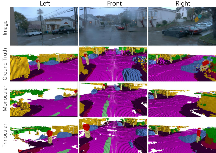
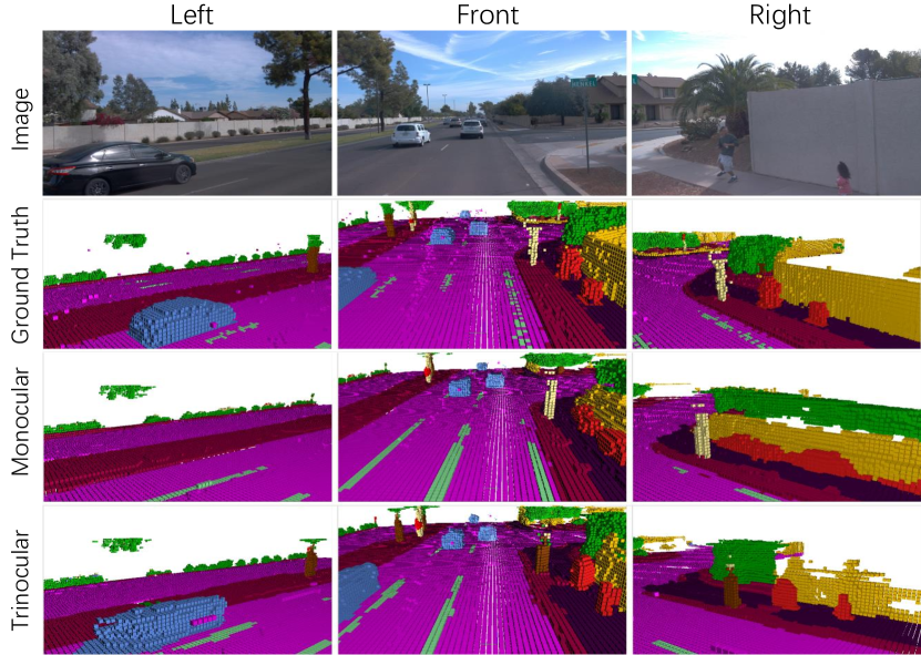
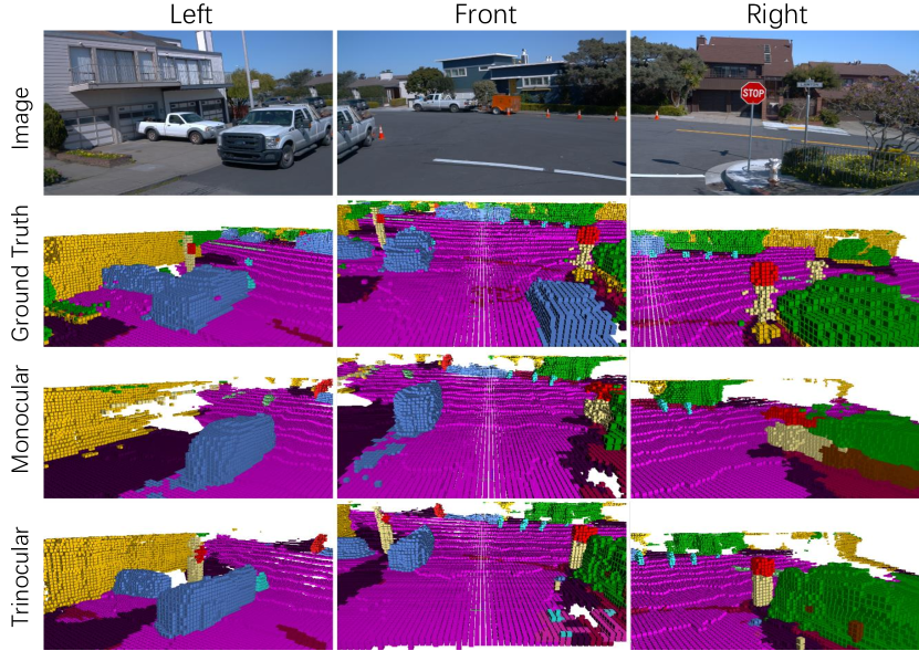
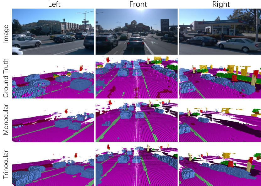
We present the necessary licenses in Appendix B, because our benchmark is constructed based on the previous works (Liao et al., 2022; Caesar et al., 2020; Sun et al., 2020). We also exhaustively analyze the impact of perception distance on the evaluation performance in Appendix C, where we present detailed results comparison from short-range to long-range under different settings. In Appendix D, we display representative qualitative visualization results from our SSCBench, along with the input image and LiDAR. Finally, the visualization comparison between the monocular method and trinocular method has also been presented in Appendix D for better qualitative evaluation.

Appendix B Dataset Details

Complying with the original dataset we used, different parts of the SSCBench dataset are released under different licenses. In particular:

•

SSCBench-KITTI-360: CC BY-NC-SA 3.0
•

SSCBench-nuScenes: CC BY-NC-SA 4.0
•

SSCBench-Waymo: Waymo Dataset License Agreement for Non-Commercial Use

The authors bear all responsibilities for the licensing, distribution, and maintenance of our datasets.

To improve the usability and readability of our SSCBench, we will release the complete dataset and detailed configurations upon acceptance, along with the codes and corresponding models for the evaluation methods on our SSCBench, based on their official codebases.

Appendix C Analysis of Range

We report the performances across three distinct scales of volume, namely 12.8 $\times$ 12.8 $\times$ 6.4m³, 25.6 $\times$ 25.6 $\times$ 6.4m³, and 51.2 $\times$ 51.2 $\times$ 6.4m³. These scales have been deliberately selected and provide an in-depth analysis of performance across varying perception ranges. Such an understanding is paramount for a variety of subsequent tasks, especially those associated with vehicle planning and navigation (Hu et al., 2023). Notably, all the aforementioned scales lie within the observable range of onboard sensors, such as cameras and LiDAR. The design choice of our evaluation from short-range to long-range underscores its significance in assessing the vehicle’s forward anticipation and the associated implications on performance in relation to the perception range.

C.1 Per Subset

In Tab. I, II, and III, comprehensive performances of the proposed three subsets SSCBench-KITTI-360, SSCBench-nuScenes, and SSCBench-Waymo have been demonstrated, especially for the three distinct evaluation ranges. As the perception range expands, all LiDAR-based and camera-based methods generally experience a decrease in performance due to increased complexity and uncertainty in larger volumes. However, LiDAR-based methods, specifically in SSCBench-Waymo, demonstrate minimal performance degradation. This trend, likely attributed to the dense LiDAR input, highlights their ability to maintain stable performance across varying perception ranges. It underscores the potential benefits of dense LiDAR data collection, albeit with increased cost and computational demand. Additionally, this trend emphasizes the need for further research to enhance LiDAR data density and advance depth estimation for camera-based methods, improving their scalability to larger perception ranges.

C.2 Trinocular vs. Monocular

Mirroring the degradation with SSCBench-Waymo, trinocular setting can also confront a decrease in performance along with the increase of evaluation range, shown in Tab. IV. However, it is worth noting that while trinocular method exhibits a comparable decline in geometric metrics (IoU) to that of monocular method, it experiences a more pronounced deterioration in semantic metrics (mIoU). One possible explanation might be that trinocular method becomes more reliant on semantic information due to the influx of additional visual information from triple inputs. As the evaluation range expands, there is a potential misalignment in the features from the visual data captured by the cameras heading to different view angles, which can have a more adverse effect on the recognition of distant objects.

C.3 Unified Benchmark Results

Table V, VI, and VII demonstrate the cross-domain evaluation across three different evaluation ranges, following the unified setting mentioned above. It is noteworthy that for LMSCNet, after training on SSCBench-KITTI-360 and testing on SSCBench-Waymo, there is a subtle improvement in performance as the evaluation distance increases. This is likely attributed to the denser LiDAR data in the SSCBench-Waymo. While a similar trend can be observed for SSCNet, a distinction emerges when trained on SSCBench-Waymo and tested on SSCBench-360: SSCNet demonstrates greater robustness to the change of distance compared to LMSCNet, which is likely due to the aforementioned number of parameters. Interestingly, for MonoScenes, the model showcases an insensitivity to the evaluation range across different datasets. Specifically, the semantic metric (mIoU) for MonoScenes experiences a decline of less than 1%.

Table I: Quantitative comparison on SSCBench-KITTI-360. We report the performances with respect to different ranges (12.8m, 25.6m, and 51.2m). We provide both geometric (IoU) and semantic (mIoU) metrics. The top three performances are marked by red, green, and blue respectively.

Methods	TPVFormer			OccFormer			VoxFormer-S			MonoScene			LMSCNet			SSCNet
Range (m)	12.8	25.6	51.2	12.8	25.6	51.2	12.8	25.6	51.2	12.8	25.6	51.2	12.8	25.6	51.2	12.8	25.6	51.2
IoU (%)	56.56	46.83	40.22	58.71	47.96	40.27	55.45	46.36	38.76	54.65	44.70	37.87	65.34	57.43	47.35	70.97	62.96	53.58
Precision (%)	68.14	62.41	59.32	69.47	62.68	59.7	66.10	61.34	58.52	65.88	59.96	56.73	77.14	73.07	72.77	78.17	72.25	69.63
Recall (%)	76.90	65.21	55.54	79.13	67.12	55.31	77.48	65.48	53.44	76.24	63.72	53.26	81.03	72.85	57.55	88.52	83.05	69.92
mIoU	22.50	18.03	13.64	23.04	18.38	13.81	18.17	15.4	11.91	20.29	16.18	12.31	20.04	17.57	13.65	24.01	21.40	16.95
car (2.85%)	36.70	30.60	21.56	40.87	33.1	22.58	29.41	25.08	17.84	30.83	26.35	19.34	37.49	31.71	20.91	50.02	44.47	31.95
bicycle (0.01%)	3.40	2.07	1.09	1.94	1.04	0.66	2.73	1.73	1.16	1.94	0.83	0.43	0.00	0.00	0.00	0.00	0.00	0.00
motorcycle (0.01%)	5.17	2.51	1.37	1.03	0.43	0.26	1.97	1.47	0.89	3.25	1.30	0.58	0.00	0.00	0.00	1.02	0.36	0.17
truck (0.16%)	17.72	12.94	8.06	22.4	15.21	9.89	6.08	6.63	4.56	14.83	12.18	8.02	0.65	0.46	0.26	14.67	13.69	10.29
other-veh. (5.75%)	5.78	4.74	2.57	8.48	6.12	3.82	3.71	3.56	2.06	6.08	4.30	2.03	1.49	1.01	0.58	0.00	0.00	0.00
person (0.02%)	3.60	3.19	2.38	4.54	3.79	2.77	2.86	2.20	1.63	2.06	1.26	0.86	0.00	0.00	0.00	0.26	0.13	0.07
road (14.98%)	73.31	65.73	52.99	73.34	66.53	54.3	66.10	58.58	47.01	68.60	59.93	48.35	77.35	74.32	62.95	78.03	75.96	65.70
parking (2.31%)	28.38	18.35	11.99	30.91	20.25	13.44	18.44	13.52	9.67	24.32	16.4	11.38	25.56	20.43	13.51	29.60	24.51	17.33
sidewalk (6.43%)	48.06	39.79	31.07	49.76	41.3	31.53	38.00	33.63	27.21	44.43	36.05	28.13	51.20	44.42	33.51	56.60	51.40	41.24
other-grnd(2.05%)	6.07	5.28	3.78	5.62	5.45	3.55	4.49	4.04	2.89	5.76	4.82	3.32	0.41	0.32	0.20	6.88	5.36	3.22
building (15.67%)	50.45	43.11	34.83	53.65	44.86	36.42	41.12	38.24	31.18	45.40	40.60	32.89	58.66	54.08	43.67	62.14	54.04	44.41
fence (0.96%)	9.40	7.68	4.8	10.64	7.85	4.8	8.99	7.43	4.97	9.79	5.91	3.53	1.66	0.71	0.33	13.53	11.06	6.77
vegetation (41.99%)	45.49	35.73	30.08	49.91	37.96	31	45.68	35.16	28.99	42.98	32.75	26.15	55.87	48.52	40.01	59.28	51.96	43.72
terrain (7.10%)	31.25	22.02	17.52	34.63	24.99	19.51	24.70	18.53	14.69	31.96	21.63	16.75	41.96	34.15	26.80	40.80	34.84	28.87
pole (0.22%)	11.82	9.74	7.46	12.93	10.25	7.77	8.84	8.16	6.51	9.28	8.45	6.92	0.00	0.00	0.00	1.09	1.19	0.78
traf.-sign (0.06%)	11.17	8.49	5.86	14.25	12.37	8.51	9.15	9.02	6.92	8.58	7.67	5.67	0.00	0.00	0.00	0.90	1.16	0.75
other-struct. (4.33%)	11.72	8.98	5.48	13.81	11.04	6.95	10.31	7.02	3.79	9.18	6.76	4.20	9.87	7.09	3.63	14.80	12.98	8.60
other-obejct (0.28%)	5.48	3.59	2.70	8.96	6.71	4.6	4.40	3.27	2.43	5.86	4.49	3.09	0.0028	0.0007	0.0003	1.13	1.07	0.67

Table II: Quantitative comparison on SSCBench-nuScenes. All metrics and legends follow those in Tab. I.

Methods	OccFormer			VoxFormer-S			MonoScene			LMSCNet			SSCNet
Range	12.8m	25.6m	51.2m	12.8m	25.6m	51.2m	12.8m	25.6m	51.2m	12.8m	25.6m	51.2m	12.8m	25.6m	51.2m
IoU (%)	62.48	42.94	28.23	59.75	39.25	25.16	65.06	44.79	29.63	61.40	36.98	21.09	63.44	43.06	27.64
Precision (%)	86.77	73.99	60.08	85.48	72.33	53.11	88.83	75.95	60.64	92.89	86.48	83.12	84.22	68.89	59.21
Recall (%)	69.05	50.57	34.75	66.5	46.18	32.34	70.84	52.09	36.69	64.03	39.25	22.03	72.00	53.45	34.14
mIoU	14.24	10.75	7.55	8.89	7.05	4.96	18.89	13.59	9.60	22.4	14.19	8.36	25.7	18.24	11.84
car (2.47%)	28.20	21.29	14.61	8.23	7.65	4.95	21.95	14.86	10.17	38.62	24.29	14.74	38.36	27.04	18.06
bicycle (0.16%)	6.97	3.57	2.25	0.26	0.38	0.29	4.13	2.39	1.70	0.00	0.00	0.00	0.00	0.00	0.00
motorcycle (0.02%)	12.22	10.29	7.97	1.56	1.99	1.21	5.86	5.72	3.80	0.00	0.00	0.00	2.24	0.77	0.36
truck (0.96%)	22.26	17.05	11.88	4.06	4.05	2.73	17.18	11.55	8.35	18.40	10.32	5.93	26.67	18.89	13.42
other-veh. (7.87%)	18.84	15.31	9.80	5.17	4.13	2.45	18.51	11.87	8.74	17.58	13.28	8.52	20.01	14.85	10.35
person (0.24%)	16.08	8.74	5.87	2.53	1.71	1.12	10.65	5.66	3.72	13.22	6.37	3.41	18.15	12.25	7.59
road (36.97%)	70.52	54.74	37.62	48.79	36.19	23.94	70.60	54.59	38.77	63.39	40.82	24.14	65.28	45.49	28.74
sidewalk (8.30%)	37.57	28.43	18.63	17.22	14.45	10.14	32.75	23.03	14.74	26.10	14.29	7.55	35.46	23.23	12.65
other-grnd (0.75%))	35.58	27.39	19.76	8.56	6.52	4.06	28.86	19.94	12.58	26.90	15.29	8.40	34.63	22.00	12.65
building (21.17%)	10.30	9.77	9.05	2.62	2.30	3.97	5.28	6.51	7.23	36.77	28.94	18.56	35.83	30.44	21.05
vegetation (20.97%)	12.09	7.63	5.92	7.62	5.18	4.58	10.79	6.90	5.50	27.87	16.74	9.02	31.81	23.91	16.33
other-obejct (0.11%)	0.00	0.00	0.00	0.02	0.05	0.06	0.29	0.06	0.03	0.00	0.00	0.00	0.00	0.02	0.01

Table III: Quantitative comparison on SSCBench-Waymo. All metrics and legends follow Tab. I.

Methods	TPVFormer			VoxFormer-S			MonoScene			LMSCNet			SSCNet
Range	12.8m	25.6m	51.2m	12.8m	25.6m	51.2m	12.8m	25.6m	51.2m	12.8m	25.6m	51.2m	12.8m	25.6m	51.2m
IoU (%)	61.59	45.07	36.78	60.36	44.09	36.36	62.44	45.36	36.81	89.19	89.19	89.04	85.26	85.34	85.43
Precision (%)	75.65	60.57	51.53	75.95	62.90	52.00	79.03	63.16	52.11	94.83	94.84	94.74	88.62	88.71	88.83
Recall (%)	76.81	63.78	56.24	75.03	59.58	54.72	74.84	61.67	55.62	93.75	93.73	93.67	95.74	95.74	95.7
mIoU	13.85	13.16	10.91	9.65	10.11	9.46	12.39	12.26	10.54	39.10	39.05	38.58	42.37	42.17	41.63
car (7.65%)	20.57	19.01	15.24	14.60	17.13	14.58	18.18	17.82	14.54	74.13	74.99	75.21	68.05	69.36	69.97
bicycle (0.02%)	0.89	1.52	1.54	0.13	0.38	0.36	0.91	0.72	1.36	0.00	0.00	0.00	17.04	14.70	13.23
motorcycle (0.001%)	0.03	0.10	0.23	0.00	0.05	0.02	0.04	0.14	0.03	0.00	0.00	0.00	0.00	0.00	0.00
person (0.84%)	9.14	6.34	4.88	8.59	6.61	5.20	12.76	9.23	6.59	61.47	59.75	58.22	61.13	60.00	58.32
bycyclist (0.03%)	2.08	4.91	2.90	0.95	2.73	1.83	0.61	3.23	3.01	0.16	0.26	0.19	15.13	15.81	15.37
road (29.62%)	64.75	53.21	43.02	63.07	49.46	40.79	66.34	53.71	42.51	76.19	76.77	76.29	75.07	75.65	75.40
sidewalk (6.65%)	31.96	28.02	22.31	18.77	18.01	17.26	26.57	24.14	19.82	51.53	50.96	51.07	52.07	51.75	51.63
other-grnd(11.40%)	22.16	21.65	19.78	8.05	13.17	15.68	17.45	20.42	18.96	51.29	51.49	51.30	51.90	52.15	52.12
building (18.38%)	10.30	14.75	13.53	1.71	5.59	10.33	7.78	13.48	12.55	72.08	72.01	71.63	70.61	70.51	70.15
lane-marking (1.15%)	20.47	18.10	14.78	11.93	15.42	13.86	12.19	15.51	14.43	10.63	10.19	9.12	14.67	14.33	13.15
vegetation (22.41%)	14.28	13.24	12.75	9.72	9.72	11.34	10.03	10.18	11.48	73.67	73.55	73.30	71.06	71.03	70.93
trunk (0.90%)	2.69	3.31	2.53	2.14	2.95	2.49	3.35	3.52	2.88	35.01	35.06	34.69	35.80	35.83	35.89
pole (0.72%)	1.77	3.18	2.96	1.52	3.19	3.10	2.88	3.79	3.48	42.23	42.47	41.58	42.34	42.21	41.88
traf.-sign (0.19%)	1.71	2.32	2.53	2.06	3.08	2.71	4.13	3.74	3.59	28.63	28.78	27.24	35.21	34.51	33.07
other-obejct (0.03%)	4.99	7.70	4.65	1.50	4.18	2.38	2.7	4.21	2.94	9.54	9.46	8.83	25.46	24.65	23.28

Table IV: Comparison between monocular and trinocular setup on SSCBench-Waymo. In the monocular setup, we only use front camera images. However, in the trinocular setup, we utilize 3 camera images, which collectively provide a 180^∘ view.

Methods	TPVFormer-Mono			TPVFormer-Tri
Range	12.8m	25.6m	51.2m	12.8m	25.6m	51.2m
IoU (%)	61.59	45.07	36.78	65.03	49.38	39.06
Precision (%)	75.65	60.57	51.53	76.76	64.40	54.65
Recall (%)	76.81	63.78	56.24	80.98	67.92	57.79
mIoU	13.85	13.16	10.91	20.62	18.07	13.71
car (7.65%)	20.57	19.01	15.24	35.56	28.57	20.62
bicycle (0.02%)	0.89	1.52	1.54	6.58	3.21	2.27
motorcycle (0.001%)	0.03	0.10	0.23	0.29	0.18	0.09
person (0.84%)	9.14	6.34	4.88	21.74	14.89	9.41
bycyclist (0.03%)	2.08	4.91	2.90	4.56	6.94	3.59
road (29.62%)	64.75	53.21	43.02	67.94	58.06	47.07
sidewalk (6.65%)	31.96	28.02	22.31	40.72	35.88	26.53
other-grnd(11.40%)	22.16	21.65	19.78	27.02	27.83	23.67
building (18.38%)	10.30	14.75	13.53	18.06	21.20	17.91
lane-marking (1.15%)	20.47	18.10	14.78	22.97	21.65	16.73
vegetation (22.41%)	14.28	13.24	12.75	24.02	22.39	18.28
trunk (0.90%)	2.69	3.31	2.53	10.51	8.20	4.84
pole (0.72%)	1.77	3.18	2.96	12.09	9.48	5.98
traf.-sign (0.19%)	1.71	2.32	2.53	7.29	5.71	4.25
other-obejct (0.03%)	4.99	7.70	4.65	9.97	6.93	4.35

Table V: Cross-domain evaluation of LMSCNet (Roldao et al., 2020). We report the experiment results of training and testing on different datasets using unified labels. Each dataset name is color-highlighted for clearer reading.

Training dataset	SSCBench-KITTI-360						SSCBench-Waymo
Testing dataset	SSCBench-KITTI-360			SSCBench-Waymo			SSCBench-KITTI-360			SSCBench-Waymo
Range	12.8m	25.6m	51.2m	12.8m	25.6m	51.2m	12.8m	25.6m	51.2m	12.8m	25.6m	51.2m
IoU (%)	67.44	58.85	48.49	16.06	16.28	17.45	8.44	5.89	4.12	89.80	89.80	89.59
Precision (%)	75.60	74.90	74.82	19.86	20.22	21.81	22.99	25.62	27.24	95.73	95.73	95.63
Recall (%)	81.53	73.31	57.95	45.62	45.54	46.63	11.76	7.10	4.62	93.55	93.54	93.42
mIoU	32.84	28.69	22.48	1.71	1.75	1.83	2.41	1.59	1.04	52.42	52.41	51.98
vehicle	41.87	35.37	23.87	0.37	0.41	0.36	3.82	2.35	1.34	75.62	75.56	76.56
bicycle	0.00	0.00	0.00	0.00	0.00	0.00	0.00	0.00	0.00	0.00	0.00	0.00
motorcycle	0.00	0.00	0.00	0.00	0.00	0.00	0.00	0.00	0.00	0.00	0.00	0.00
person	0.00	0.00	0.00	0.00	0.00	0.00	0.07	0.03	0.03	65.23	64.23	62.69
road	78.45	75.47	64.04	4.07	4.19	4.02	3.15	2.34	1.65	79.70	80.33	79.96
sidewalk	53.53	46.61	35.13	0.84	0.86	0.82	0.75	0.36	0.19	52.42	52.29	52.37
other-grnd	30.05	25.41	17.46	2.31	2.36	2.77	1.81	1.34	0.90	52.37	52.44	52.27
building	60.71	54.30	44.47	2.31	2.36	2.74	6.42	5.17	4.03	72.97	72.95	72.45
vegetation	58.65	49.69	39.75	9.19	9.35	9.99	8.05	4.22	2.19	75.47	75.28	74.94
other-obejct	0.16	0.07	0.04	0.01	0.00	0.00	0.06	0.10	0.06	50.49	50.02	48.54

Table VI: Cross-domain evaluation of SSCNet (Song et al., 2017).

Training dataset	SSCBench-KITTI-360						SSCBench-Waymo
Testing dataset	SSCBench-KITTI-360			SSCBench-Waymo			SSCBench-KITTI-360			SSCBench-Waymo
Range	12.8m	25.6m	51.2m	12.8m	25.6m	51.2m	12.8m	25.6m	51.2m	12.8m	25.6m	51.2m
IoU (%)	70.98	63.56	54.50	16.79	16.99	17.82	10.52	9.01	8.99	85.83	85.86	85.89
Precision (%)	76.88	72.21	70.07	22.83	23.20	24.58	25.01	27.19	30.43	89.26	89.30	89.31
Recall (%)	90.25	84.13	71.03	38.85	38.82	39.31	15.37	11.87	11.31	95.70	95.71	95.72
mIoU	35.03	31.68	25.63	4.18	4.20	4.18	3.00	2.07	1.33	51.59	51.51	51.31
vehicle	49.54	44.31	34.14	3.92	3.69	3.11	7.00	4.62	2.73	69.80	71.00	71.55
bicycle	0.00	0.00	0.00	0.00	0.00	0.00	0.00	0.00	0.00	6.57	5.43	5.65
motorcycle	0.00	0.00	0.00	0.00	0.00	0.00	0.00	0.00	0.00	0.00	0.00	0.00
person	0.43	0.19	0.11	0.00	0.00	0.00	0.09	0.05	0.04	61.96	60.94	60.26
road	79.71	77.76	67.54	4.24	4.12	3.47	4.05	2.67	1.73	78.37	78.97	78.65
sidewalk	58.95	53.18	41.84	1.62	1.65	1.47	0.94	0.49	0.27	53.42	53.10	53.11
other-grnd	33.70	28.96	19.86	2.39	2.37	2.31	1.32	0.75	0.50	52.88	53.17	53.02
building	64.49	57.39	46.89	16.96	17.42	18.20	7.11	7.16	5.53	70.53	70.47	70.17
vegetation	61.66	53.99	44.92	12.10	12.20	12.77	9.39	4.82	2.46	72.13	72.03	71.99
other-obejct	1.79	1.66	1.01	0.59	0.55	0.44	0.05	0.10	0.07	50.22	49.95	48.73

Table VII: Cross-domain evaluation of MonoScene (Cao & de Charette, 2022).

Training dataset	SSCBench-KITTI-360						SSCBench-Waymo
Testing dataset	SSCBench-KITTI-360			SSCBench-Waymo			SSCBench-KITTI-360			SSCBench-Waymo
Range	12.8m	25.6m	51.2m	12.8m	25.6m	51.2m	12.8m	25.6m	51.2m	12.8m	25.6m	51.2m
IoU (%)	57.39	46.81	39.11	11.68	9.7	7.07	16.03	13.41	14.72	63.37	46.1	54.61
Precision (%)	70.86	64.27	60.84	19.13	15.13	11.95	28.70	25.18	25.20	80.18	64.18	53.46
Recall (%)	75.11	63.28	52.26	23.07	21.38	14.74	26.64	22.30	26.14	75.14	62.07	54.61
mIoU	32.01	25.43	19.53	2.84	2.78	2.16	2.56	2.47	2.28	18.17	17.37	14.67
vehicle	35.27	29.50	21.29	6.07	8.6	9.87	1.24	1.18	0.98	20.59	20.08	16.09
bicycle	7.59	3.89	2.60	0.54	0.15	0.01	0.00	0.00	0.00	3.83	3.29	2.03
motorcycle	7.01	3.02	1.60	0.00	0.00	0.00	0.00	0.00	0.00	0.00	0.17	0.09
person	6.36	4.54	3.27	1.23	1.76	2.12	0.00	0.00	0.00	14.28	9.86	6.82
road	73.02	64.39	51.62	3.44	4.02	2.99	13.14	8.48	6.58	69.66	57.12	46.31
sidewalk	48.87	39.37	30.42	1.14	0.95	0.55	3.80	2.51	0.19	32.46	28.31	23.14
other-grnd	30.39	21.08	14.25	0.56	0.65	0.24	1.94	2.85	2.37	19.27	22.87	20.92
building	51.44	43.12	34.83	5.78	3.28	0.45	0.76	4.23	5.11	5.21	14.23	13.7
vegetation	48.24	36.48	29.16	8.92	7.70	5.00	2.82	4.20	5.26	13.66	13.89	13.9
other-obejct	11.95	8.88	6.26	0.74	0.63	0.38	0.01	0.01	0.02	2.73	3.86	3.65

Appendix D Qualitative Results

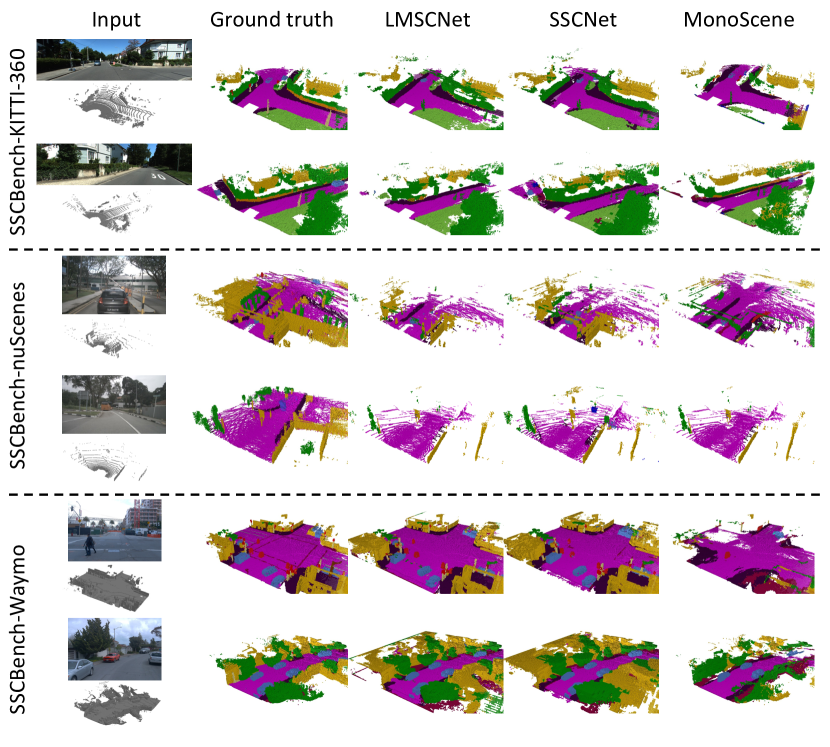
In Fig. I, we show the completion results of different methods on the SSCBench dataset. We can observe comparable results between LMSCNet (Roldao et al., 2020) and SSCNet (Song et al., 2017), while MonoScene (Cao & de Charette, 2022) has a varying performance depending on the input. On SSCBench-KITTI-360, MonoScene has comparable results to the two LiDAR-based methods due to the large FOV. It also shows a superior completion ability when there is occlusion near the ego-vehicle (see the 3rd row). However, when the FOV is limited, MonoScene fails to predict the scene outside the visible input (the last two rows). Additionally, in order to qualitatively analyze results under different camera settings, We show the comparison of semantic scene completion results between monocular and trinocular methods on our proposed SSCBench-Waymo dataset, as Fig. II, III, IV and V. Benefiting from the more visual input of the supplementary perspectives, trinocular method can also have a better perception of the environment next to the ego vehicle. Moreover, multi-view input also contributes to more reasonable reasoning for the front view, especially the details in long-range, as shown in the second column of Fig. II.

SSCBench: Monocular 3D Semantic Scene Completion Benchmark in Street Views