Scale-awareness in an eddy energy constrained mesoscale eddy parameterization
Abstract
There is an increasing interest in mesoscale eddy parameterizations that are scale-aware, normally interpreted to mean that a parameterization does not require parameter recalibration as the model resolution changes. Here we examine whether Gent–McWilliams (GM) based version of GEOMETRIC, a mesoscale eddy parameterization that is constrained by a parameterized eddy energy budget, is scale-aware in its energetics. It is generally known that GM-based schemes severely damp out explicit eddies, so the parameterized component would be expected to dominate across resolutions, and we might expect a negative answer to the question of energetic scale-awareness. A consideration of why GM-based schemes damp out explicit eddies leads a suggestion for what we term a splitting procedure: a definition of a ‘large-scale’ field is sought, and the eddy-induced velocity from the GM-scheme is computed from and acts only on the large-scale field, allowing explicit and parameterized components to co-exist. Within the context of an idealized re-entrant channel model of the Southern Ocean, evidence is provided that the GM-based version of GEOMETRIC is scale-aware in the energetics as long as we employ a splitting procedure. The splitting procedure also leads to an improved representation of mean states without detrimental effects on the explicit eddy motions.
Journal of Advances in Modeling Earth Systems (JAMES)
Department of Ocean Science, Hong Kong University of Science and Technology Center for Ocean Research in Hong Kong and Macau, Hong Kong University of Science and Technology National Oceanography Centre, Southampton School of Mathematics and Maxwell Institute for Mathematical Sciences, The University of Edinburgh Department of Physics, University of Oxford Department of Physics, The Chinese University of Hong Kong
Julian Makjulian.c.l.mak@googlemail.com
Evidence is presented for scale-awareness of the GEOMETRIC eddy parameterization with a ‘splitting’ approach
Scale-awareness means constancy of total eddy energy, while the explicit and parameterized components vary with resolution
In eddy permitting calculations, such eddy parameterizations should be applied to the large-scale background state, obtained via ‘splitting’
Plain Language Summary
With increasing computational power, ocean models are starting to explicitly resolve eddy motions with characteristic length-scales of 10 to 100 km. With the increased model resolution, there is an increasing call for scale-aware parameterizations, i.e. simplified models that are supposed to represent the missing eddy feedbacks onto the modeled state that are either self-tuning, or do not require re-tuning of parameters, without damping explicit eddies resolved by the model. The question we ask is whether an eddy parameterization known as GEOMETRIC is scale-aware. The expected answer might be “no”: such schemes are known to heavily flatten density variations and damp out explicitly resolved eddies. We instead propose a splitting scheme that avoids damping of explicitly resolved eddies. The GEOMETRIC scheme, with the use of splitting, seems to be scale-aware in the sense that there is approximate constancy of total eddy energy, where the explicit and parameterized components vary with resolution, and additionally lead to other desirable features in the model considered.
1 Introduction
The ocean is a central component of the Earth system, and changes in the overturning circulation have important consequences for the global energy and biogeochemical cycles [<]e.g.,¿ZhangVallis13, Adkins13, Ferrari-et-al14, Burke-et-al15, Bopp-et-al17, Takano-et-al18, GalbraithdeLavergne19, Li-et-al20. In particular, it is known that the representation of geostrophic mesoscale eddy processes in numerical models, whether explicitly permitted by the numerical model or through a parameterization, can have a significant influence on the ocean climate sensitivity [<]e.g.,¿FoxKemper-et-al19, Hewitt-et-al20.
Models employing parameterizations often require “tuning”, or parameter calibration, in that the paramaeters associated with the parameterizations are adjusted so that the model reduces known biases of the model, such as sea surface temperature patterns, overall Southern Ocean volume transport, or mixed layer depths, relative to a high resolution model truth and/or observational data. On the other hand, with increasing computational power, there is an increasing possibility for numerical ocean models to increase in spatial resolution. With an increased horizontal resolution the geostrophic mesoscale motion starts becoming explicitly represented, which is known to offer some benefits over parameterizations, such as improvements to global/regional biases in the relevant ocean metrics, such as those mentioned above [<]e.g.,¿Hewitt-et-al17, Hewitt-et-al20. While there is an increasing push for the so called -scale (kilometer scale) models that aim to explicitly resolve the eddy dynamics and dispense with parameterizations altogether [Slingo \BOthers. (\APACyear2022), Hewitt \BOthers. (\APACyear2022)], such models are computationally prohibitive for climate applications, which tend to require long-time integrations. A more realistic and achievable goal in the near future is for ocean models used for climate projections to be eddy permitting, at roughly horizontal resolution, where the modeled eddy-mean feedback is known to be insufficient, and some form of parameterization is still required for the missing eddy feedbacks. It is generally beneficial to have a traceable hierarchy of numerical models differing mostly in the resolution [<]e.g.,¿Storkey-et-al18, to tackle the appropriate questions in a computationally tractable manner depending on the time or spatial scales of interest.
With such a hierachy of models, there is an increasing interest in scale-aware parameterizations, in that one set of parameter choice is applicable across model resolutions. Examples of these include parameterizations based on Large Eddy Simulations designed for rotating stratified turbulence, with a resulting eddy viscosity/diffusion that is grid-scale dependent [<]e.g.,¿Smagorinsky93, Bachman-et-al17b. On the other hand, more traditional parameterizations, such as the Gent–McWilliams (GM) scheme [Gent \BBA McWilliams (\APACyear1990), Gent \BOthers. (\APACyear1995)], isoneutral diffusion [<]e.g.,¿Redi82, Griffies-et-al98, enhanced vertical momentum diffusion [<]e.g.,¿GreatbatchLamb90, and backscatter [<]e.g.,¿Zanna-et-al17, Bachman19, Jansen-et-al19, Juricke-et-al20, are based on Reynolds averaging procedures. The first three cases and variants thereof normally rely on a specification of a diffusivity or a transfer coefficient and are generally not scale-aware by construction, although there are proposals to make these schemes scale-aware, such as via a resolution function that scales the diffusivity according to the modeled state [<]e.g.,¿Hallberg13. Backscatter schemes, where a portion of the energy dissipated at the grid-scale or other means is re-injected back into the resolved scales, is scale-aware in the sense that the scheme itself dynamically adjusts depending on the model length-scales (be it the grid-scale, effective resolution based for example on the Rossby deformation radius, or otherwise).
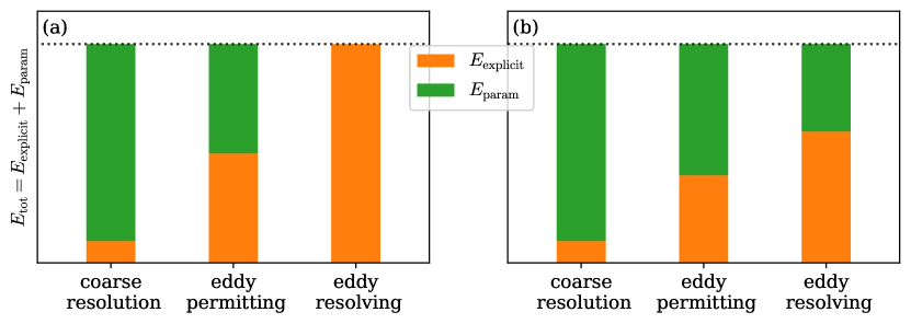
The principal focus of this work is on GM-based parameterizations, valid for geostrophic mesoscale motions for which the Rossby number is small. With the increased prevalence of eddy energy constrained GM-based parameterizations [<]e.g.,¿EdenGreatbatch08, MarshallAdcroft10, Marshall-et-al12, Jansen-et-al19, an aspect that we consider in this work is scale-awareness in the total eddy energy. We suppose that there is a fixed amount of total eddy energy available, but this can be represented in explicit or parameterized forms. The question here is whether an energetically constrained eddy parameterization is scale-aware in the eddy energetics, in the sense that total (explicit and parameterized) eddy energy is conserved as model resolution is varied without re-tuning of parameters, while the partition into explicit and parameterized components may vary. An ideal scenario we envisage would be where the parameterized eddy energy decreases while the explicit component increases as resolution increases, such that the sum remains constant, as illustrated in Fig. 1(). The eddy resolving model has all the eddy energy in the explicit component, and explicit eddies are responsible for all the eddy-mean interaction. The coarse resolution models are tuned so that the total eddy energy is roughly the same as the eddy resolving model, but most of the eddy energy contribution is in the parameterized component. Without additional tuning, as we go into the eddy permitting regime, some of that work by parameterized eddies are taken up by the explicit eddies, but such that the total eddy energy remains constant. This could be possible with energetically constrained parameterizations, since the resolved modeled state information is often utilized in the parameterized eddy energy budgets, but by no means guaranteed. An alternative and more plausible (but still desirable) scenario might be that illustrated in Fig. 1(), where the parameterized component reduces in magnitude but does not completely vanish as we move from the coarse through eddy permitting to eddy resolving resolutions. Without further tuning, there may still be a non-negligible amount of eddy energy in the parameterized component, but this might be regarded as scale-aware since the total eddy energy level is still roughly constant.
For this work we focus on one of the existing eddy energy constrained mesoscale eddy parameterizations, the GM-based version of GEOMETRIC [<]e.g.,¿Marshall-et-al12, Mak-et-al18, which has been implemented and tested in various numerical ocean general circulation models in a variety of configurations [<]e.g.,¿Mak-et-al18, Mak-et-al22, Ruan-et-al23. The principal question we address in the present article is whether GEOMETRIC, without the use of resolution functions or backscatter, is itself scale-aware in terms of the eddy energetics. A reasonable first guess at the answer would be “no”: the GM-based schemes are intended for calculations at non-eddying resolutions, and are known to severely damp any mesoscale eddies that are explicitly represented in eddy permitting models. An example of this excessive damping is shown in Fig. 2(), where the use of GM-based schemes as standard in a 25 km horizontal resolution model (to be introduced in §2) severely damps the instantaneous fluctuations, as represented by the surface relative vorticity, relative to Fig. 2() where no GM-based scheme is active. The use of the GM-based schemes as-is puts us firmly in the regime where the parameterized component is almost entirely responsible for the eddy-mean interaction and occupies a large percentage of the total eddy energy, and in this instance we would not expect scale-awareness.
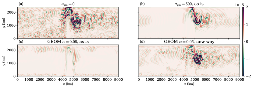
In §2 we review the reasons why GM-based schemes damp explicit eddies, suggesting what we term here a splitting procedure that would enable GM-based schemes (not necessarily just GEOMETRIC) to avoid damping explicit eddy activity; see Fig. 2() for an example of GEOMETRIC employing the splitting procedure. A splitting procedure puts us in the regime where parameterized and explicit eddies may in principle co-exist without intruding on one another. Being constrained by an overall eddy energy budget that depends on the resolved mean-state, GEOMETRIC could be scale-aware in the eddy energetics. The presence or absence of explicit eddies would lead to variations in the resolved mean-state that is expected to impact the parameterized eddy energy. The parameterized eddy feedback onto the resolved mean-state is dependent on the parameterized eddy energy, and the parameterized eddy feedback might adjust according to the level of explicit eddy feedback. The exact implementation of the splitting procedure and the numerical experiments for testing whether we have energetic scale-awareness in GEOMETRIC are detailed in §3. §4 provides evidence in support of GEOMETRIC having scale-aware energetics, and further examines other benefits offered by the splitting procedure, focusing on the model in the eddy permitting regime with a horizontal resolution of 25 km (roughly ). We close the article in §5 where we discuss the results, provide outlooks, as well as the practical and modeling implication for the splitting procedure detailed in this work, such as the use of a resolution function and backscatter parameterizations.
2 The GM scheme and the splitting approach
2.1 GM scheme currently as applied
The GM scheme, while resembling a horizontal buoyancy diffusion [<]in the quasi-geostrophic limit, e.g.,¿Treguier-et-al97 or a layer thickness diffusion [<]e.g.,¿GentMcWilliams90, is really an advection [<]e.g.,¿Gent-et-al95, Treguier-et-al97, Griffies98, Ferreira-et-al05, and introduces an eddy-induced velocity as
| (1) |
Here, denotes the unit vector pointing in the vertical direction, encodes the isopycnal slopes in the horizontal directions, is the dynamically relevant density, the horizontal gradient operator, and is the GM or the eddy-induced velocity coefficient. The GM scheme only adds the eddy-induced velocity to the tracer equations: assuming that the only thermodynamic variable is the temperature , the active tracer equation is modified to
| (2) |
where is the resolved velocity, and the right-hand-side includes the relevant forcing, diffusion and/or dissipation terms. The eddy-induced velocity as represented by the GM scheme acts to flatten isopycnals, originally intended to mimic the action of baroclinic instability. In practice it ends up leading to a parameterized interfacial form stress regardless of the generating mechanism, since meridional advection of buoyancy/density is equivalent to a vertical transfer of horizontal momentum in the quasi-geostrophic limit [<]e.g.,¿GreatbatchLamb90, McWilliamsGent94, Marshall-et-al12.
The GM scheme was originally designed for models with no explicit eddies, where the isopycnal slope is a fundamentally large-scale field with no small-scale fluctuations in both the velocity and density (the two variables being related via the thermal wind shear relation). Having GM-based schemes switched on when explicit eddies are permitted severely damps the explicit eddies. The reason for this is essentially given in Eq. (1): with explicit eddies in regimes where thermal wind balance holds, the resulting isopycnal slope has small-scale fluctuations, so that the resulting eddy-induced velocity is potentially large magnitude at small-scales, via a curl of . The resulting acts to rapidly damp the smaller-scale explicit fluctuations that are permitted. If the magnitude of is large, the resulting model calculation strongly resembles a coarse resolution model with no explicit eddies (cf. Fig. 2, and sample calculations not shown with spatially constant but large ). On the other hand, while the calculation with no GM-based scheme switched on looks better and possesses stronger explicit fluctuations, the mean state turns out to be slightly problematic, attributed to the explicit eddy feedback onto the mean-state being too weak (e.g., the stratification and circumpolar transport associated with the Fig. 2 calculation will be seen to be too deep and too strong respectively). It would appear that some form of parameterization is required to supplement the missing eddy-mean interaction.
Several approaches have been proposed to combat the excessive damping and to increase the eddy impact on the mean state, and are sometimes used in combination. One is to consider an anisotropic version of the GM parameterization, where the anisotropy refers to the along and across stream direction [<]e.g.,¿SmithGent04, although this is not commonly implemented. Another is to control the value of based on a grid spacing and/or the Rossby deformation radius of the resolved state [<]e.g.,¿Hallberg13, and the GM scheme is thus only functioning where the state is regarded as ‘under-resolved’. Yet another is via a momentum-based backscatter approach [<]e.g.,¿Zanna-et-al17, Bachman19, Jansen-et-al19, Juricke-et-al20, which aims to model the pathway of energy flowing towards large-scales associated with rotationally constrained turbulence [<]e.g.,¿Charney71, Rhines75, Salmon80, VallisMaltrud93, SrinivasanYoung12, WatermanJayne12, and has the benefit of energizing the explicit flow. One possible critique with the use of a resolution function is that controlling affects the magnitude but not the small-scale nature of , and the GM scheme is still applied outside of its intended domain of validity. A possible criticism of the damping first then backscatter approach is that it risks compensating overly strong dissipation with overly strong backscatter, leading to two balancing or competing unphysical mechanisms. For example, the strong small-scale dissipation of a direct application of GM at eddy permitting resolution does not correspond to large-scale baroclinic instability, but instead to the parameterization being used outside of its intended regime of validity. While physical eddy backscatter is observed and is a target for parameterization, it should not be confused with numerical backscatter acting to counter excessive dissipation.
2.2 A field splitting approach
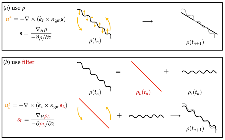
Given the previous discussion alluding to large/small-scale fields, the proposal here is to consider an approach motivated by the schematic given in Fig. 3. Given an appropriate definition of a large-scale density field , where , we compute the associated large-scale isopycnal slope . The associated eddy-induced velocity is computed using , i.e.
| (3) |
and we might apply this only to the large-scale active tracer equations.
This proposal might be expected to address the critique that GM is being used beyond its regime of validity and the excessive damping that is observed when using GM in eddy permitting regimes. Since is a large-scale field by construction, the resulting will also be large-scale, at least much larger-scale than the scales associated with the explicit eddies using a suitable definition. As a corollary, since is a curl of a large-scale rather than small-scale field, we would expect . The present proposal thus controls both the spatial distribution and the magnitude of the eddy-induced velocity, and is perhaps closer in spirit to the original intention of the GM scheme [Gent \BBA McWilliams (\APACyear1990), Gent \BOthers. (\APACyear1995)], that is, a parameterization on a background that has no eddies, here defined by a large-scale field that has the explicit eddy field filtered out in some way.
The present proposal supplements the explicit interfacial form stress with some parameterized form stress computed only using the large-scale field, but in a way that aims to avoid cancellations through competing effects. By comparison, controlling aims to avoid excessive dissipation completely, while GM-based schemes with backscatter would dissipate first and, accepting that there is cancellation, add back some of the missing parts. That said, the present proposal is not mutually exclusive of additional controls on , nor on the use of backscatter. We would argue that, with the present splitting approach, no control on is strictly necessary, since this is already taken care of by the use of . Already damping fewer eddies, such a scheme would imply that, when used in conjunction with backscatter, the degree of backscatter might not need to be that substantial.
The splitting approach here does not require substantial modification of the relevant GM-based schemes themselves, since only the data used in computing the relevant quantities are modified. There are of course various theoretical and practical aspects to consider, such as (1) the choice of filter, (2) the relevant large-scale tracer equations to implement, (3) issues with nonlinear equation of state, (4) computational cost issues, and others. These are further discussed in §3 where we detail the precise implementation choices considered in this work, and in §5 where we evaluate of our choices and provide possible alternative.
2.3 Parameterized eddy energetics
The splitting approach detailed above makes no specific choice of GM-based scheme, and to address the question of whether there is eddy energy scale-awareness, in that the total (explicit and parameterized) eddy energy remains somewhat constant with changing model resolution, we focus our attention on the GM-based version of the GEOMETRIC scheme [Marshall \BOthers. (\APACyear2012), Mak \BOthers. (\APACyear2018), Mak, Marshall\BCBL \BOthers. (\APACyear2022)]. The GM-version of GEOMETRIC arises from a bound via analyzing the Eliassen–Palm flux tensor [Marshall \BOthers. (\APACyear2012), Maddison \BBA Marshall (\APACyear2013)] in the quasi-geostrophic regime, and results in a with a linear dependence on the total eddy energy . The implementation of \citeAMak-et-al22 in a global configuration ocean global circulation model takes
| (4) |
where is the total (potential and kinetic) parameterized eddy energy, prognostically determined by the parameterized eddy energy budget
| (5) |
Here, the depth-integrated total parameterized eddy energy is advected by the depth-averaged flow , with westward propagation at the long Rossby wave phase speed [<]e.g.,¿Chelton-et-al11, KlockerMarshall14. The growth of parameterized eddy energy comes from the slumping of mean density surfaces, where and are the horizontal and vertical buoyancy frequencies (so ). The parameterized eddy energy is diffused in the horizontal [Grooms (\APACyear2015), Ni, Zhai, Wang\BCBL \BBA Hughes (\APACyear2020), Ni, Zhai, Wang\BCBL \BBA Marshall (\APACyear2020)] with a diffusivity . A linear dissipation of the parameterized eddy energy at rate is employed (with minimum parameterized eddy energy level ), so is an time-scale, and is a bulk parameterization of energy fluxes out of the mesoscales resulting from numerous dynamical processes [<]e.g.,¿Mak-et-al22b.
One question here is on the nature of the quantities to be used in Eq. (4) and Eq. (5) if we consider employing a splitting approach detailed above. To maintain a positive-definite source term, we utilize
| (6) |
where the subscript denotes the quantities computed using the large-scale density field , and the form of the source term is supported by an analysis analogous to that in Appendix A of \citeAMak-et-al17a. While there is no obvious restriction as such on the computation of in Eq. (4), it would be more consistent that we also use large-scale information, i.e., in employing as given in Eq. (3), we also compute
| (7) |
so that the resulting is a large-scale field.
3 Implementation and model set up
As a first implementation to test out the idea of scale-awareness in the eddy energetics and the splitting approach, we make some simplifications to what was proposed in §2 and Fig. 3. Specifically, we consider (1) a filtering performed per horizontal level, and (2) the resulting is applied to the full tracer equation. The first is not an unreasonable first approximation given we are dealing with systems with small aspect ratios, and we normally expect the isopycnal slopes to be rather small. While we would ideally like to define a large-scale based on some sort of isopycnal-based averaging, a horizontal average at fixed depth is maybe a reasonable first attempt, at least numerically. The second is more of a theoretical issue, where we would in this instance like to derive an equation only for the large-scale active tracer field, which is not an immediately obvious endeavor because of the definition of the velocity; some ideas and discussions are provided in §5. If however it is the case that the use of a large-scale field already leads to a large-scale and small magnitude , we might expect that the small-scales are advected in a somewhat passive manner by , and it is possible that in practice the expected reduction in damping may already allow the scale-awareness in eddy energetics (if it exists) to emerge.
3.1 Implementation in NEMO
A natural way to filter fields might be to consider a diffusion-based filter. Taking the tracer variable to be temperature for concreteness, consider the diffusion equation discretized in time given by
| (8) |
where denotes a length-scale squared, is a nominal diffusivity, and would be a nominal time-step size. Here the superscripts on denote the pseudo-time index, and the idea here is to pseudo-time-step a full field into some large-scale field as dictated by the diffusion operator. If we take the right hand side to be at pseudo-time index , then we are dealing with an explicit scheme that, while easy to code up, is subject to strong constraints on the choice of through stability conditions. One could consider repeated cycling via for some , but in practice needs to be quite large for finer resolution models because the choice of stable is rather small, and we lose the interpretability of as a length-scale.
We consider instead
| (9) |
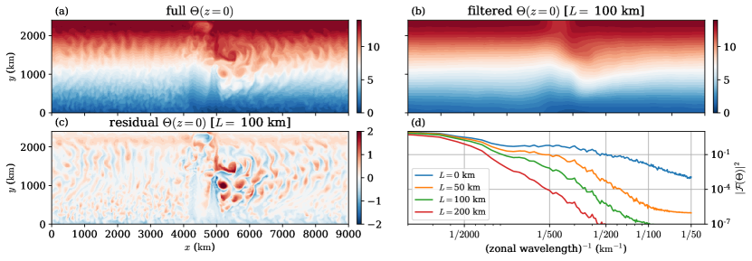
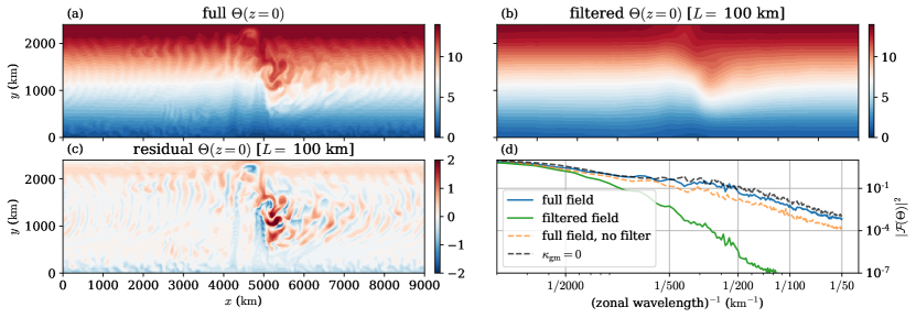
which bears resemblance to solving the diffusion equation by a backward Euler scheme, except with the exponent on the operator . Dealing with implicit schemes alleviates the constraint placed by stability conditions and can in principle be chosen independent of the choice of model resolution. The operator in this case is symmetric positive-definite, so there are a variety of solvers available [<]e.g., conjugate gradient;¿Leveque-ODEs. The choice of for the exponent follows the technical arguments given in A that the operator has an associated Green’s function with a characteristic length-scale for the choice of , such that may be interpreted as a filter length-scale (e.g., the power spectrum falling off beyond some the length-scale ). Fig. 4 shows the filter in action. Note in particular that the zonal power spectrum of the large-scale field at fixed latitude (averaged over all latitudes) shown in Fig. 4() shows a power drop off to below that coincides with the choice of as long as it is bigger than the Nyquist wavelength of the model (which is for the dataset concerned).
The present implementation for the filter employs a Richardson iteration
[<]e.g.,¿Richardson10, Trottenberg-et-al-Multigrid with a pre-conditioning
with parameter , which was easier to implement in NEMO and suffices for
the cases considered; see A for details. Within NEMO itself, a new
module called ldftra_split was introduced to perform the filtering
procedure, leveraging a substantial amount of existing code for computing
diffusive trends associated with the discretized Laplacian operator (e.g.,
traldf_lap_blp). If we are letting the relevant eddy-induced velocity
act on the total tracer field (i.e. solving for
Eq. 2) then no further modifications except for the computation of
the relevant quantities are required. The addition of operations in NEMO is
roughly:
-
•
if splitting, call
tra_ldf_splitprovided by new moduleldftra_split, resulting in a large-scale thermodynamic fieldtsb_l; -
•
use
tsb_lto recompute the related stratification variables (rab_b,rn2b,rhd) after the vertical physics step (which uses the full thermodynamic fieldtsb); -
•
compute the slopes
wslp[ij]using the recomputedrhdandrn2b; -
•
rhdis recomputed using fulltsbfor ocean physics (NEMO already does this call by default); -
•
call GEOMETRIC routines in
ldfeke, where newwslp[ij]are used to obtain eddy induced velocitiesaei[uv], and these are exposed to the tracer advection modulestraadvas usual.
The relevant data redirection are all performed in the NEMO time-stepping driver
module step; see the source files provided as part of the open data
repository (search for tra_ldf_split and tsb_l in
step.F90).
3.2 Model setup
The above procedures were implemented in NEMO 4.0.5 (r14538), and tested in an idealized zonally re-entrant channel model of the Southern Ocean. The model set up is based on that of \citeAMunday-et-al15, with no continental barriers but with a submerged ridge, and is a longer version of the channel model in \citeAMak-et-al18. The model domain is 9000 km by 2400 km by 3000 m in the zonal, meridional and vertical direction, the choice of domain extent is such that models with horizontal grid spacing of , , and km are supported (denoted here by R100, R050, R025, R010 respectively). The model employs a linear bottom drag with coefficient . Specifications of the submerged ridge (the domain is at 1500 m depth at its most shallow), the purely zonal and time-independent wind stress forcing (with peak wind stress at ) as well as the surface temperature restoring profile are the same as \citeAMunday-et-al15 and \citeAMak-et-al18, adapted to the present domain.
The model takes a linear equation of state with temperature as the only thermodynamic variable. There is a constant vertical diffusivity everywhere in the domain, except in a km sponge region towards the northern boundary where the value of is increased towards in the same manner described in \citeAMunday-et-al15 and \citeAMak-et-al18. The choice of enhanced diffusivity differs to restoring northern boundary conditions considered for example in \citeAAbernathey-et-al13 and \citeAYoungs-et-al19, and has an impact on the residual meridional overturning circulation. Given the choice of a single thermodynamic variable, no isoneutral diffusion [Redi (\APACyear1982), Griffies \BOthers. (\APACyear1998)] is employed. All models detailed below employ a lateral hyperdiffusion in the temperature field, chosen as , where for all calculations, and except for R100 where to damp out the grid-scale fluctuations. The hyper viscosities where employed follow the same prescription but with ; the Laplacian viscosity for R100 was chosen empirically. A summary of the key model parameters are given in Table 1.
Three sets of experiments were performed. One set has no GM-based parameterization switched on (denoted , neglecting units). One set has the GEOMETRIC parameterization switched on and applied as standard (employing Eq. 4 and 5). The final set and the principal focus of the present work is the one with the GEOMETRIC parameterization but with a splitting approach (Eq. 6 and 7). All calculations were spun up from rest at the relevant horizontal resolutions with to the end of model year 500, and perturbation experiments were performed from start of model year 501 to end of model year 810, where the time-averaging period is the last 10 years (start of model year 801 to end of model year 810). All the GEOMETRIC-based calculations here employ the same parameter values, given in Table 1; the choice of and is on the larger side to previous reported works, but the value of is not inconsistent with the estimates for the Southern Ocean derived from an inverse calculation [Mak, Avdis\BCBL \BOthers. (\APACyear2022)].
| Parameter | R100 | R050 | R025 | R010 | Units | |
|---|---|---|---|---|---|---|
| grid spacing | 100 | 50 | 25 | 10 | ||
| time step size | 60 | 40 | 20 | 10 | ||
| viscosity | 5000 | — | — | — | ||
| hyper-viscosity | — | |||||
| hyper-diffusivity | ||||||
| filter length scale | — | 100 | 100 | 100 | ||
| pre-conditioning param. | — | 20 | 75 | 500 | — |
| Parameter | Common values | Units | |
|---|---|---|---|
| eddy efficiency | 0.06 | — | |
| energy diffusivity | 500 | ||
| minimum energy level | 4.0 | ||
| dissipation time-scale | 80 | days |
The choice of the GEOMETRIC parameters (principally and , respectively the coefficient related to the growth and dissipation of parameterized eddy energy) were chosen as follows. We first perform a model truth calculation R010 with . We diagnose the total explicit eddy energy as the sum of domain-averaged eddy kinetic energy
| (10) |
where is a time average over the 10 year window, is the volume of the computation domain, denotes the bathymetry, and denotes the domain extents in the zonal and meridional directions. The domain-averaged eddy potential energy is computed in density co-ordinates as
| (11) |
where is the density computed from the linear equation of state. Both of the above quantities were computed from five-day averaged data output every five days over the 10 year window. The and parameters were tuned roughly so that the coarse resolution model R100 possesses similar total (explicit and parameterized) eddy energy levels and total circumpolar transport to the model truth calculation. The circumpolar transport is calculated as
| (12) |
where denotes the time-averaged zonal velocity.
For the results presented here all splitting was performed with the aforementioned filter with fixed length-scale of , and the pre-conditioning parameter was determined empirically as the value that leads to a stable convergence of the Richardson iteration procedure in a Python implementation of the filtering algorithm (see file provided in data repository). For computation cost reasons, however, the filtering procedure is only performed every model day, although the small-scale field (being the residual of the total and large-scale field) is updated at every time-step. A mild defense of this choice is that the large-scale spatial varying field is expected to be slowly evolving in time [<]cf.¿Rai-et-al21, and an update at every model time-step may not be strictly necessary. Sample experiments varying the update period from every time-step to every model month did not lead to any noticeable differences in the resulting conclusions of this article. With the current choice of updating every model day, the extra run time given the same amount of computational resources was empirically determined to be no more than 5% for the R025 calculations.
4 Results
As described in previous works [<]e.g.,¿Munday-et-al15, Mak-et-al18, the model is characterized by a flow arising from blocked contours because of the submerged ridge, where is Coriolis parameter. The mean flow deflects towards the north (or equator), and downstream of the ridge a standing meander and substantial mesoscale eddy activity results; see for example the snapshots of the surface relative vorticity shown previously in Fig. 2(). The resulting Rossby deformation radius as measured by [<]cf.¿NurserBacon14 varies in latitude from 5 to about 100 km from south to north, and has a domain-average of around ; in that sense R010 is resolving eddies except far into the south, R025 is eddy-permitting, R050 is barely eddy-permitting, and R100 is non-eddy resolving. In the model truth R010 with , the diagnosed total circumpolar transport (Eq. 12) is 115.0 Sv (where 1 Sv = ), with a domain averaged specific total eddy energy of all in the explicit component (where about 20% of this is in the form of EKE). The R100 coarse resolution calculation employing GEOMETRIC has the and roughly tuned to the aforementioned transport and eddy energy values, and the resulting calculation with the parameters given in Table 1 has total circumpolar transport of 118.8 Sv and a domain averaged specified eddy energy of , where the latter is a little high compared to the model truth. About 32% of the coarse resolution total eddy energy is in the explicit EPE, and the remaining essentially in the parameterized eddy energy, with a negligible amount in the explicit EKE.
4.1 Scale-awareness in the energetics
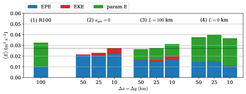
The information regarding the eddy energy across the set of calculations across resolutions is summarized in Fig. 5. In the calculations, the total eddy energy increases with resolution as expected, with most of the explicit eddy energy as EPE that remains roughly constant with increasing resolution, and a notable increase in the explicit EKE. It should be noted that the R050 and R025 (the models in the ‘eddy permitting’ regime) with have a stratification that is extended too deep compared to the model truth (e.g., Fig. 7 later), with too large a transport compared to the model truth.
In the calculations employing a filtering with the use of GEOMETRIC and , there is a suggestion that the total eddy energy (parameterized and explicit) is somewhat constant, indicating scale-awareness in the eddy energetics, although a non-negligible amount of the total eddy energy is in the parameterized component. The total explicit eddy energy component (in both EKE and EPE form) is certainly lower in comparison to the corresponding calculations, but is noticeably higher than the calculations where GEOMETRIC is used as is with no filtering of fields (particularly noticeable in the explicit EKE levels).
We note that there is a significant component of total eddy energy in the parameterized component across the resolutions. A major contribution to the parameterized eddy energy seems to be the presence of the standing meander. The standing meander is persistent (albeit substantially weakened) under the filtering, contributing to significant generation of parameterized eddy energy that leads to damping of the explicit component via the associated eddy-induced velocity, so that the parameterization ends up compensating for the reduced eddy activity. Analogous model calculations without a ridge and so no standing meander (not shown) also results in rough constancy of total eddy energy, but with a substantially decreased parameterized component as resolution is increased (cf. Fig. 1). The results suggest we may want to consider filtering procedures that remove or reduce the projection of the standing eddy onto the large-scale field; choices of the filter and the definition of a large-scale field are further discussed in the conclusion section.
We should note that the eddy energy dependence behavior discussed here seem to be robust with reasonable variations of GEOMETRIC parameters and with the present choice of filtering length scale , for sample sets of calculations that have been performed (not shown), as long as the total circumpolar transport is roughly around 115 Sv ( say).
4.2 Mean state sensitivities
To further investigate the impact of the splitting procedure in the set of calculations, we take the R025 calculations as a working example to demonstrate a few desirable features conferred to the model that results from the present procedure; similar conclusions appear to hold in the R050 calculations (not shown).
The reduced damping of the explicit eddies is apparent already in the snapshots of the surface relative vorticity shown previously in Fig. 2(). In the filtered variable, Fig. 6 shows a snapshot of the sea surface temperature field diagnosed from a prognostic calculation of R025 with GEOMETRIC and splitting active (in contrast to Fig. 4, which demonstrates the filtering procedure on a snapshot of a diagnosed tracer field from a calculation). The model large-scale field has a persistent zonal temperature gradient near the location of the ridge, arising from the projection of the standing meander onto the large-scale field. A substantial amount of activity is in the small-scales, as seen in Fig. 6(), demonstrating that the filtering and splitting procedure functions even in a prognostic setting (which is not immediately obvious given the nonlinear feedbacks present in contrast to the filtering applied diagnostically). To quantify the explicit activity, the zonal power spectrum of the sea surface temperature at fixed latitudes averaged over latitudes is shown in Fig. 6(). The power spectrum density in the large-scale decreases (the green line) to a magnitude of at the filtering length-scale (cf. Fig. 4). The power spectrum density of the full field from the present calculation (the blue line) is smaller across scales but otherwise reasonable compared to a calculation of R025 with (the black dashed line), indicating a mild decrease in explicit activity in R025 calculations with GEOMETRIC and the splitting procedure. The analogous power spectrum for a calculation with no filtering (the orange dashed line) is smaller than the two aforementioned cases by about an order of magnitude for length-scales smaller than around .
A sample set of the zonal mean temperature and zonal velocity profiles is given in Fig. 7. It can be seen here that while R100 has a comparable total zonal transport (of around 115 Sv) to the model truth R010 with , their stratification differs, with the R100 calculations having a stratification extending deeper (Fig. 7). This observation is reflected in the diagnosis of a thermal wind or baroclinic transport
| (13) |
where is given by Eq. (12), and the second term is the transport associated with the bottom flow (in practice being taken at the first wet point above the modeled bathymetry). R100 with the present choice of GEOMETRIC parameters has Sv, while the model truth R010 has Sv. The stronger depth-independent component with the increased resolution as mesoscale eddies are resolved is consistent with the findings of \citeAYankovsky-et-al22.
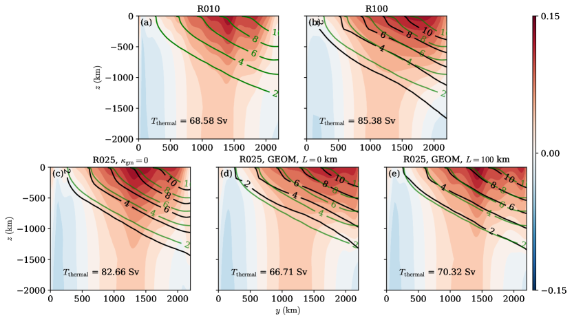
For the R025 calculations, we note that the calculations (Fig. 7), while showing the most variability (Fig. 2 and Fig. 6), has a deeper zonal mean stratification profile compared to the model truth R010, consistent with Sv in this calculation. The calculation employing GEOMETRIC but no splitting (Fig. 7) leads to a zonal mean stratification that has mismatches in the deeper regions, although the thermal wind transport is comparable to the model truth, with Sv. Note the substantially weaker variations in the zonal mean zonal velocity in the GEOMETRIC without splitting calculation, consistent with the strong damping of the present model seen in the snapshots (cf. Fig. 2). The calculation with GEOMETRIC and splitting (Fig. 7) leads to a zonal mean stratification, a baroclinic transport of Sv and a zonal mean flow that is meridionally confined, all of which agrees well with the model truth calculation. Further, the zonal mean zonal velocity also possesses more spatial fluctuations, consistent with the reduced damping of the explicit eddies. The splitting approach in this calculation allows the extra flattening of isopycnals arising from the GM-based GEOMETRIC scheme, but with only very mild damping of the explicit fluctuations. The similar diagnosed values of in the R025 cases considered is likely due to the better resolved standing eddy over the ridge; similar observations are seen in the analogous R010 calculations, though less so in the R050 set of calculations.
The calculation with splitting appears to allow both the explicit and parameterized eddy-mean feedbacks to be present, and provides the most satisfactory representation of the zonal mean stratification and zonal mean flow, while maintaining a degree of variability not present with standard implementations of GM-based schemes. It should additionally be noted that the agreement in the stratification appears to require the splitting procedure to be active. In our sample calculations of R025 employing GEOMETRIC (not shown), we find that for fixed (since changes in the mean state from can be offset accordingly by inverse changes in ), we can certainly tune so that the total or baroclinic transport agree with the model truth, but biases in the stratification appear to be persistent (e.g., inspecting the isopyncal contours visually). In that sense, there is some evidence lending support to the conclusion that the splitting approach really does lead to a better represented mean state – a mean state that standard procedures struggle to replicate by tuning. Analogous calculations in a model without a ridge results in a similar conclusion, but with the R025 calculation having an even deeper stratification (not shown), attributed to the fact there is no longer form stress contributions from the standing eddy to the momentum budget.
A set of wind perturbation experiments were performed by multiplying the zonally symmetric wind stress by a constant factor, again starting from the start of model year 501 to the end of model year 810, for the model truth R010 with , R025 with , and R025 with GEOMETRIC using the splitting procedure. Fig. 8 shows the diagnosed total transport and thermal wind transport calculated from the time-averaged data in the same analysis period (start of model year 801 to end of model year 810). The model truth R010 with has a mildly decreasing baroclinic transport with increasing wind before rebounding somewhat at very large wind forcing (four times the control wind stress). The sensitivity of transport was previously observed in the shorter channel model of \citeAMak-et-al18, and possibly arises from the use of an enhanced vertical diffusivity in the northern boundary, leading to a residual overturning in the opposite direction to the usual one [Youngs \BOthers. (\APACyear2019)].
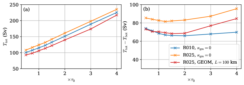
The R025 case with follows the decreasing trend in the baroclinic transport of the model truth for moderate winds, but increases again at larger winds. The overall sensitivity in the thermal wind transport with changes in wind stress however is substantially weaker than the calculations in a non-eddying calculation R100 using a constant [<]not shown, but cf. Fig. 1 of¿Mak-et-al18, likely because of the improved representation of form stress when some eddies are permitted [<]cf.¿Munday-et-al13, and also because the standing meander is better resolved [Stewart \BOthers. (\APACyear2022)]. For the R025 case employing GEOMETRIC and splitting, the thermal wind transport follows the trend of the model truth well up to twice the control wind forcing, but increases significantly at larger wind forcing. To rationalize the observed behavior, note that both the transient and standing eddy play a role in the momentum balance via their role in vertical momentum transport. With splitting, where there is a degree of separation between the explicit and parameterized eddies, with the latter increasing with wind forcing as describe by GEOMETRIC, the explicit standing eddy is still only partially resolved, leading to differing sensitivity to that observed in the model truth. On the other hand, in the cases without splitting [<]e.g. R100; cf.¿Mak-et-al18, or a case considered by accident here with splitting but where parameterized eddy energy advection by the mean flow was essentially inactive, the parameterized component intrudes on the explicit eddy and takes over its role to various degrees in the momentum budget, leading to different sensitivities (almost eddy saturated, with very weak dependence of thermal wind transport with increases in wind stress; not shown). The present observations further highlight the importance and ongoing challenges in representing the eddy-mean feedback from the standing eddy, be it explicitly or via a parameterization.
5 Conclusions and outlooks
An aim of this work is to re-examine whether it is possible to achieve a more physical representation of mesoscale eddy feedback with existing parameterization schemes, for use in the next generation of eddy-permitting ocean models. To that end, the primary question we consider here is whether the GM-based version of GEOMETRIC is scale-aware in the energetics, in that the total (parameterized plus explicit) eddy energy remains roughly constant over different spatial resolutions, without recalibration of parameters. Within the context of an idealized re-entrant channel model as a representation of the Southern Ocean, the diagnosed total eddy energy levels shown in Fig. 5 provides evidence that the GM-based version of GEOMETRIC is in fact scale-aware, as long as a splitting approach based on filtering is utilized so that the parameterized component does not completely dominate the total eddy feedback. As the explicit eddies become stronger with increased horizontal resolution, the resulting explicit feedback is reflected in the large-scale state, which affects the growth of the parameterized eddy energy (Eq. 6), modifying the resulting distributions such that the parameterized eddy component “makes way” for the explicit eddy component, and vice-versa. While we might have expected that the splitting approach would allow the parameterized and explicit eddy component to exist side by side, it was still not obvious that the GM-based version of GEOMETRIC would necessarily be scale-aware, so the present finding is by no means trivial. The scale-awareness is demonstrated for one choice of the GEOMETRIC parameters (see Table 1), where the choice was chosen so that the resulting total transport and total eddy energy levels roughly coincides with the model truth calculation. The scale-awareness result seems to be robust across sample sets of calculations (with different GEOMETRIC parameters, and analogous model calculations in the absence of a topographic ridge) as long as the resulting total transport of the coarse resolution model was roughly that of the model truth, differing only in the total eddy energy levels and in the exact partition of the explicit and parameterized eddy energy. In addition to scale-awareness, the splitting approach leads to various improvements to eddy permitting models that are also non-trivial, such as reducing bias in the mean stratification profiles without sacrificing the dynamical fluctuations (e.g., Fig. 7), and improving on the transport values and possibly on its sensitivities (e.g., Fig. 8).
The principle behind the splitting approach advocated here is summarized in Fig. 3: we would like to split out a large-scale non-eddying state from the full state via a filter, compute an eddy-induced velocity from the resulting large-scale non-eddying state, and apply the resulting only to the large-scale state. The resulting as computed is an inherently large-scale and smaller magnitude object, which avoids damping the explicitly resolved small-scale eddies, and is closer to the original intention and derivation of \citeAGentMcWilliams90 via a Reynolds averaging procedure. For this first work, two simplifications were made in the proposed splitting approach that differs from the schematic given in Fig. 3, namely (1) a horizontal filtering rather than a filtering along-isopycnals, and (2) the eddy-induced velocity acts on the full tracer field. The first is partly justified in that we are in the small aspect ratio regime where the horizontal average serves as a reasonable first approximation to along-isopycnal averaging; the horizontal average utilizes a filtering (see Eq. 9) with a well-defined length-scale (fixed to be in this work). The second is for simplicity, and we expect that since is a large-scale field with suitable choices of the filter, the small-scales are already somewhat passively advected by the eddy-induced velocity, so would allow scale-awareness to emerge. The scale-awareness in the eddy energetics as shown in Fig. 5 with the present approach we would expect to be improved by further refinements to the procedure.
The splitting procedure, while still employing a variant of the more standard isotropic advection provided by the GM scheme, removes a modeling need for a resolution function [<]e.g.,¿Hallberg13, which modifies the value of directly, with impact on the resulting eddy-induced velocity ; for this work and our particular choice of filter, the resolution scale is replaced by the definition of filtering length-scale . We also note that the existing splitting approach is agnostic to the choice of the GM-based scheme itself. Here we happen to choose the GM-based GEOMETRIC scheme, so there are some subtleties with the parameterized eddy energetics that one has to be careful about (see §2.3). The analysis however places no restriction on the exact specification of , and could be used with other GM-based variants [<]e.g.,¿Visbeck-et-al97, Treguier-et-al97, EdenGreatbatch08, Jansen-et-al15a, Jansen-et-al15b, Jansen-et-al19. In addition, the splitting approach is not mutually exclusive with backscatter parameterizations [<]e.g.,¿Zanna-et-al17, Bachman19, Jansen-et-al19, Juricke-et-al20, and some backscatter would even be preferable to energize the explicit flow and capture physical backscatter mechanisms. We would however make a note that, since the explicit eddies themselves are not strongly damped in the splitting approach, the degree of backscatter likely does not need to be so large. It would be of interest to see if the GM-based GEOMETRIC scheme (or indeed other existing mesoscale eddy parameterizations) in the presence of backscatter would still be scale-aware in the energetics, but this is beyond the scope of the present work.
In the present work we made the choice of studying scale-awareness in relation to the eddy energetics, when others have considered the total (mean and eddy) energetics [<]e.g.,¿Jansen-et-al19. We have analyzed the mean kinetic energy and see that similar conclusions regarding scale-awareness appear to hold, although we note that in the present model the domain-integrated mean kinetic energy is smaller than the total eddy energy by about an order of magnitude. Similar observations in the ratio between kinetic energy of depth-averaged component and the residual baroclinic component to \citeAYankovsky-et-al22 also hold, in both the mean and eddy component (not shown). However, compared to the mean kinetic energy, the computation for mean potential energy is more troublesome, since the reference for available potential energy is in general difficult to compute [<]e.g.,¿Tailleux13, HieronymusNycander15, SuIngersoll16, particularly for data from a -level model. In this work we made the choice to focus on the eddy energetics because the references are well-defined for eddy energetics, and present only results for eddy energetics for consistency reasons.
We make some further comments to our two simplifications made in this present work. Starting with the splitting procedure, the present work employs a filter per horizontal level given by Eq. 9, with a well-defined length-scale , where for this work we took . With a decreased (e.g., ), the splitting becomes incomplete and we somewhat return into the regime where the parameterized component dominates. For larger (e.g., ), the parameterized component becomes weak in the intermediate resolution calculations R025 and R050, leading to a deviation from total eddy energy constancy. For the present choice of filter, two elliptic solves are required, but since the filtering procedure is only carried out every model day, the computation costs are rather minimal and empirically determined to be no more than 5% extra run time in the R025 calculations, possibly improved further with a better solver. Sample calculations show no noticeable impact on the resulting calculations even if the splitting procedure was carried out once every month, which could be attributed to the fact that the large-scale field is unlikely going to evolve on a fast time-scale.
On a side point relating to large-scale field evolving on a slower time-scale, the Reynolds averaging procedure in deriving the GM-scheme would be more appropriate using a time-based averaging. Employing a spatial filter as we have done here is implicitly assuming that there is some equivalency between a time and space averaging, and is only really valid under rather specific assumptions. There is indeed a mix of averages used interchangeably here, and while this may not be an unreasonable choice to make from a practical point of view (and is indeed used by other works to do with eddy parameterization in the literature), it is ultimately a choice that should be further examined and refined, with its impacts quantified if possible.
The quantitative details are almost certainly dependent on how the large-scale field is defined. The present work utilizes a fixed choice of filtering length-scale , but it is perfectly possible to have this as a parameter that varies in space and time, since the problem is intrinsically based on solving a diffusion-like equation. For example, choices of that are some multiple of a local Rossby deformation radius should be possible, although some modifications would presumably be required so that the pre-conditioning parameter required for numerical convergence varies with the choice of filtering length-scale. Investigations with other types of spatial filters or coarse-graining operators [<]e.g.,¿Aluie19, Grooms-et-al21 or some sort of dynamics based splitting are possible and should be considered, although we note that there are computation considerations that should be taken into account (e.g. halo sizes when parallel computation is involved, re-computation of the filtering kernel if the filtering length is to vary in time). It should also be advantageous to define some sort of operator that further removes the projection of the standing eddy onto the large-scale field. Analogous numerical calculations (not shown) removing the ridge from the modeled system, thereby removing the presence of the standing eddy, still results in rough scale-awareness in the total eddy energy as in Fig. 5, but with a more significant explicit component and a much weaker parameterized component as resolution is increased (cf. Fig. 1). Beyond a horizontal filtering as we have considered, it might be more satisfactory to consider ways to define a large-scale isopycnal surface in line with the schematic in Fig. 3, via rolling averages in the co-ordinates or other computation approaches [<]e.g.,¿Kafiabad22, KafiabadVanneste23, but is beyond the scope of the present work.
Regarding the choice here that the eddy-induced velocity is applied to the full tracer field, this is largely for simplicity reasons, with the assumption that the small-scale is advected by somewhat passively. To have the eddy-induced advection acting only on the large-scales, however, requires an equation governing the large-scale field that remains to be rigorously determined. While it is certainly possible to form a large-scale equation from the usual Reynolds averaging procedure, the problem here is in determining which velocity field should be used: should it be the total velocity, the filtered velocity, the velocity associated with the filtered thermodynamic field (via geostrophic balance for example), or something else, with additions of the eddy-induced velocity as appropriate? The highlighted issues remain to be settled.
The present work employs a linear equation of state with temperature as the only thermodynamic variable, and the filtering procedure is applied directly on the temperature field per horizontal level. Care needs to be taken when utilizing a nonlinear equation of state, since the filtered density is not the same as the density of the filtered thermodynamic variables. We propose that, with a nonlinear equation of state, it should be the neutral density that is to be filtered, from which we calculate the associated eddy-induced velocity , and apply that to the tracer equations. This might be reasonable if we continue with the approximation that is to be applied to the full tracer field, but care presumably needs to be taken for points raised in the previous paragraph if is to act on to-be-determined large-scale tracer equations. One aspect that should be examined in more detail is the degree of non-adiabaticity introduced by the present procedure. For the present case where is applied to the full tracer equation we suspect the non-adiabaticity to be rather small. A slightly more problematic aspect concerns isoneutral diffusion [Redi (\APACyear1982), Griffies (\APACyear1998)]. In this model with a single thermodynamic variable there is no isoneutral diffusion, and it is not clear with a nonlinear equation of state whether the diffusion should be along the isoneutral directions of the full isopycnals, or the large-scale isopycnals. The latter is likely going to introduce some cross isopyncal transport, while the former simply requires storing and/or re-computing the isopycnal slopes and is likely a ‘safer’ default option. Both of these issues should be addressed with a comprehensive assessment quantifying the associated impacts, but is beyond the scope of the present work.
From a practical point of view, it would be of interest to further test out the splitting procedure in different and/or more realistic ocean models, but of course bearing in mind various aforementioned subtleties that we should check for in the related investigations. An extension of the investigation in \citeARuan-et-al23 assessing the impacts of the splitting procedure to physical and biogeochemical responses in an idealized gyre model is ongoing. For more realistic global configuration models, it is known that there are various issues with the physical response with eddy permitting ocean models particularly in the Southern Ocean, such as the circumpolar transport being too large, impacting on the other connected components in the ocean such as the Southern Ocean gyres, sea ice, and on the resulting tracer transports [<]e.g.¿Hewitt-et-al20. It would be of interest to see if such a splitting procedure proposed here with the use of a GM-based GEOMETRIC scheme is able to reduce the known biases, given the efficacy of the scheme demonstrated in the present idealized Southern Ocean only ocean model, and is subject of some planned future works.
Data Availability
This work utilizes the Nucleus for European Modelling of the Ocean model [<]¿[v4.0.5, r14538]NEMO_man. The instructions on setting up the numerical model, implementation of algorithm into NEMO, model data, and scripts used for generating the plots in this article are available through the repository at \citeAMak23.
Appendix A Technical details relating to the filter
The filtering procedure employed in this work is associated with the equation
| (14) |
where is the total field to be filtered at time-step , is the filtered field, is the length-scale of choice, and in this work we take . If we have then the above is essentially a pseudo time-stepping of the diffusion equation with a backward Euler scheme. The choice of is made for several properties, such as an interpretation as a filter where the radial spectral power density decreases after a specified length-scale, or through a convolution with a kernel that has decreasing support after specified length-scale [<]e.g.,¿Whittle63, Lindgren-et-al11, and is closely related to the Matérn auto-covariance.
The operator is positive definite and symmetric, and the resulting system could be readily treated with standard methods [<]e.g., conjugate gradient;¿Leveque-ODEs. In this work we consider employing Richardson iteration [<]e.g.,¿Richardson10, Trottenberg-et-al-Multigrid, i.e.
| (15) |
where is the input field at time-step and is kept fixed as iteration number is varied, as it is easier to implement in NEMO and is sufficient for the cases considered. If the iteration by (15) converges to some , then we have the solution to Eq. (14) for the case. We repeat the outlined iteration procedure once more to obtain the solution for the case.
The method above converges if the matrix 2-norm of the discretization of is sufficiently small, which is dependent on the choice of and the grid spacing through the discretization of . To aid convergence, we consider a pre-conditioning of Eq. (15) given by [<]e.g.,¿Trottenberg-et-al-Multigrid
| (16) |
where some is an acceleration parameter chosen to ensure convergence, motivated by , where the role of is to reduce the norm of the operator. A larger is required for convergence, though it also tends to reduce the rate of convergence. The actual values used are determined empirically, and in the present calculations are given in Table 1.
In this work, the convergence criteria for the Richardson iteration is that the global supremum norm is below some tolerance, i.e.
| (17) |
For this work, since we are only filtering the temperature field, we take , and all reported calculations converged within 500 iterations. With the current choices, the extra computation costs are rather minimal, empirically determined to be no more than 5% extra run time, and possibly improved further with a better solver.
Acknowledgements.
This research was funded by both the RGC General Research Fund 16304021 and the Center for Ocean Research in Hong Kong and Macau, a joint research center between the Qingdao National Laboratory for Marine Science and Technology and Hong Kong University of Science and Technology. We thank the referees Peter Gent, Elizabeth Yankovsky and Julie Deshayes for their comments that helped clarify some scientific/algorithmic points and improve the presentation of the article.References
- Abernathey \BOthers. (\APACyear2013) \APACinsertmetastarAbernathey-et-al13{APACrefauthors}Abernathey, R., Ferreira, D.\BCBL \BBA Klocker, A. \APACrefYearMonthDay2013. \BBOQ\APACrefatitleDiagnostics of isopycnal mixing in a circumpolar channel Diagnostics of isopycnal mixing in a circumpolar channel.\BBCQ \APACjournalVolNumPagesOcean Modell.721–16. {APACrefDOI} 10.1016/j.ocemod.2013.07.004 \PrintBackRefs\CurrentBib
- Adkins (\APACyear2013) \APACinsertmetastarAdkins13{APACrefauthors}Adkins, J\BPBIF. \APACrefYearMonthDay2013. \BBOQ\APACrefatitleThe role of deep ocean circulation in setting glacial climates The role of deep ocean circulation in setting glacial climates.\BBCQ \APACjournalVolNumPagesPaleoceanography28539–561. {APACrefDOI} 10.1002/palo.20046 \PrintBackRefs\CurrentBib
- Aluie (\APACyear2019) \APACinsertmetastarAluie19{APACrefauthors}Aluie, H. \APACrefYearMonthDay2019. \BBOQ\APACrefatitleConvolutions on the sphere: Commutation with differential operators Convolutions on the sphere: Commutation with differential operators.\BBCQ \APACjournalVolNumPagesGEM: Int. J. Geomath.101–31. {APACrefDOI} 10.1007/s13137-019-0123-9 \PrintBackRefs\CurrentBib
- Bachman (\APACyear2019) \APACinsertmetastarBachman19{APACrefauthors}Bachman, S\BPBID. \APACrefYearMonthDay2019. \BBOQ\APACrefatitleThe GM+E closure: A framework for coupling backscatter with the Gent and McWilliams parameterization The GM+E closure: A framework for coupling backscatter with the Gent and McWilliams parameterization.\BBCQ \APACjournalVolNumPagesOcean Modell.13685–106. {APACrefDOI} 10.1016/j.ocemod.2019.02.006 \PrintBackRefs\CurrentBib
- Bachman \BOthers. (\APACyear2017) \APACinsertmetastarBachman-et-al17b{APACrefauthors}Bachman, S\BPBID., Fox-Kemper, B.\BCBL \BBA Pearson, B. \APACrefYearMonthDay2017. \BBOQ\APACrefatitleA scale-aware subgrid model for quasi-geostrophic turbulence A scale-aware subgrid model for quasi-geostrophic turbulence.\BBCQ \APACjournalVolNumPagesJ. Geophys. Res. Oceans1221529–1554. {APACrefDOI} 10.1002/2016JC012265 \PrintBackRefs\CurrentBib
- Bopp \BOthers. (\APACyear2017) \APACinsertmetastarBopp-et-al17{APACrefauthors}Bopp, L., Resplandy, L., Untersee, A., Le Mezo, P.\BCBL \BBA Kageyama, M. \APACrefYearMonthDay2017. \BBOQ\APACrefatitleOcean (de)oxygenation from the Last Glacial Maximum to the twenty-first century: insights from Earth System models Ocean (de)oxygenation from the Last Glacial Maximum to the twenty-first century: insights from Earth System models.\BBCQ \APACjournalVolNumPagesPhil. Trans. R. Soc. A37520160323. {APACrefDOI} 10.1098/rsta.2016.0323 \PrintBackRefs\CurrentBib
- Burke \BOthers. (\APACyear2015) \APACinsertmetastarBurke-et-al15{APACrefauthors}Burke, A., Stewart, A\BPBIL., Adkins, J\BPBIF., Ferrari, R., Jansen, M\BPBIF.\BCBL \BBA Thompson, A\BPBIF. \APACrefYearMonthDay2015. \BBOQ\APACrefatitleThe glacial mid-depth radiocarbon bulge and its implications for the overturning circulation The glacial mid-depth radiocarbon bulge and its implications for the overturning circulation.\BBCQ \APACjournalVolNumPagesPaleoceanography301021–1039. {APACrefDOI} 10.1002/2015PA002778 \PrintBackRefs\CurrentBib
- Charney (\APACyear1971) \APACinsertmetastarCharney71{APACrefauthors}Charney, J\BPBIG. \APACrefYearMonthDay1971. \BBOQ\APACrefatitleGeostrophic turbulence Geostrophic turbulence.\BBCQ \APACjournalVolNumPagesJ. Atmos. Sci.281087-1095. \PrintBackRefs\CurrentBib
- Chelton \BOthers. (\APACyear2011) \APACinsertmetastarChelton-et-al11{APACrefauthors}Chelton, D\BPBIB., Schlax, M\BPBIG.\BCBL \BBA Samelson, R\BPBIM. \APACrefYearMonthDay2011. \BBOQ\APACrefatitleGlobal observations of nonlinear mesoscale eddies Global observations of nonlinear mesoscale eddies.\BBCQ \APACjournalVolNumPagesProg. Oceanog.91167–216. {APACrefDOI} 10.1016/j.pocean.2011.01.002 \PrintBackRefs\CurrentBib
- Eden \BBA Greatbatch (\APACyear2008) \APACinsertmetastarEdenGreatbatch08{APACrefauthors}Eden, C.\BCBT \BBA Greatbatch, R\BPBIJ. \APACrefYearMonthDay2008. \BBOQ\APACrefatitleTowards a mesoscale eddy closure Towards a mesoscale eddy closure.\BBCQ \APACjournalVolNumPagesOcean Modell.20223–239. {APACrefDOI} 10.1016/j.ocemod.2007.09.002 \PrintBackRefs\CurrentBib
- Ferrari \BOthers. (\APACyear2014) \APACinsertmetastarFerrari-et-al14{APACrefauthors}Ferrari, R., Jansen, M\BPBIF., Adkins, J\BPBIF., Burke, A., Stewart, A\BPBIL.\BCBL \BBA Thompson, A\BPBIF. \APACrefYearMonthDay2014. \BBOQ\APACrefatitleAntarctic sea ice control on ocean circulation in present and glacial climates Antarctic sea ice control on ocean circulation in present and glacial climates.\BBCQ \APACjournalVolNumPagesProc. Natl Acad. Sci. USA111248753–8758. {APACrefDOI} 10.1073/pnas.1323922111 \PrintBackRefs\CurrentBib
- Ferreira \BOthers. (\APACyear2005) \APACinsertmetastarFerreira-et-al05{APACrefauthors}Ferreira, D., Marshall, J.\BCBL \BBA Heimbach, P. \APACrefYearMonthDay2005. \BBOQ\APACrefatitleEstimating eddy stresses by fitting dynamics to observations using a residual-mean ocean circulation model and its adjoint Estimating eddy stresses by fitting dynamics to observations using a residual-mean ocean circulation model and its adjoint.\BBCQ \APACjournalVolNumPagesJ. Phys. Oceanogr.351891–1910. {APACrefDOI} 10.1175/JPO2785.1 \PrintBackRefs\CurrentBib
- Fox-Kemper \BOthers. (\APACyear2019) \APACinsertmetastarFoxKemper-et-al19{APACrefauthors}Fox-Kemper, B., Adcroft, A\BPBIJ., Böning, C\BPBIW., Chassignet, E\BPBIP., Curchitser, E\BPBIN., Danabasoglu, G.\BDBLYeager, S\BPBIG. \APACrefYearMonthDay2019. \BBOQ\APACrefatitleChallenges and prospects in ocean circulation models Challenges and prospects in ocean circulation models.\BBCQ \APACjournalVolNumPagesFront. Mar. Sci.665. {APACrefDOI} 10.3389/fmars.2019.00065 \PrintBackRefs\CurrentBib
- Galbraith \BBA de Lavergne (\APACyear2019) \APACinsertmetastarGalbraithdeLavergne19{APACrefauthors}Galbraith, E.\BCBT \BBA de Lavergne, C. \APACrefYearMonthDay2019. \BBOQ\APACrefatitleResponse of a comprehensive climate model to a broad range of external forcings: relevant for deep ocean ventilation and the development of late Cenozoic ice ages Response of a comprehensive climate model to a broad range of external forcings: relevant for deep ocean ventilation and the development of late Cenozoic ice ages.\BBCQ \APACjournalVolNumPagesClim. Dyn.52623–679. {APACrefDOI} 10.1007/s00382-018-4157-8 \PrintBackRefs\CurrentBib
- Gent \BBA McWilliams (\APACyear1990) \APACinsertmetastarGentMcWilliams90{APACrefauthors}Gent, P\BPBIR.\BCBT \BBA McWilliams, J\BPBIC. \APACrefYearMonthDay1990. \BBOQ\APACrefatitleIsopycnal mixing in ocean circulation models Isopycnal mixing in ocean circulation models.\BBCQ \APACjournalVolNumPagesJ. Phys. Oceanogr.20150–155. {APACrefDOI} 10.1175/1520-0485(1990)020¡0150:IMIOCM¿2.0.CO;2 \PrintBackRefs\CurrentBib
- Gent \BOthers. (\APACyear1995) \APACinsertmetastarGent-et-al95{APACrefauthors}Gent, P\BPBIR., Willebrand, J., McDougall, T\BPBIJ.\BCBL \BBA McWilliams, J\BPBIC. \APACrefYearMonthDay1995. \BBOQ\APACrefatitleParameterizing eddy-induced tracer transports in ocean circulation models Parameterizing eddy-induced tracer transports in ocean circulation models.\BBCQ \APACjournalVolNumPagesJ. Phys. Oceanogr.25463-474. {APACrefDOI} 10.1175/1520-0485(1995)025¡0463:PEITTI¿2.0.CO;2 \PrintBackRefs\CurrentBib
- Greatbatch \BBA Lamb (\APACyear1990) \APACinsertmetastarGreatbatchLamb90{APACrefauthors}Greatbatch, R\BPBIJ.\BCBT \BBA Lamb, K\BPBIG. \APACrefYearMonthDay1990. \BBOQ\APACrefatitleOn parametrizing vertical mixing of momentum in non-eddy resolving ocean models On parametrizing vertical mixing of momentum in non-eddy resolving ocean models.\BBCQ \APACjournalVolNumPagesJ. Phys. Oceanogr.201634–1637. \PrintBackRefs\CurrentBib
- Griffies (\APACyear1998) \APACinsertmetastarGriffies98{APACrefauthors}Griffies, S\BPBIM. \APACrefYearMonthDay1998. \BBOQ\APACrefatitleThe Gent–McWilliams skew flux The Gent–McWilliams skew flux.\BBCQ \APACjournalVolNumPagesJ. Phys. Oceanogr.28831–841. {APACrefDOI} 10.1175/1520-0485(1998)028¡0831:TGMSF¿2.0.CO;2 \PrintBackRefs\CurrentBib
- Griffies \BOthers. (\APACyear1998) \APACinsertmetastarGriffies-et-al98{APACrefauthors}Griffies, S\BPBIM., Gnanadesikan, A., Pacanowski, R\BPBIC., Larichev, V\BPBID., Dukowicz, J\BPBIK.\BCBL \BBA Smith, R\BPBID. \APACrefYearMonthDay1998. \BBOQ\APACrefatitleIsoneutral diffusion in a -coordinate ocean model Isoneutral diffusion in a -coordinate ocean model.\BBCQ \APACjournalVolNumPagesJ. Phys. Oceanogr.28805–830. {APACrefDOI} 10.1175/1520-0485(1998)028¡0805:IDIAZC¿2.0.CO;2 \PrintBackRefs\CurrentBib
- Grooms (\APACyear2015) \APACinsertmetastarGrooms15{APACrefauthors}Grooms, I. \APACrefYearMonthDay2015. \BBOQ\APACrefatitleA computational study of turbulent kinetic energy transport in barotropic turbulence on the -plane A computational study of turbulent kinetic energy transport in barotropic turbulence on the -plane.\BBCQ \APACjournalVolNumPagesPhys. Fluids27101701. {APACrefDOI} 10.1063/1.4934623 \PrintBackRefs\CurrentBib
- Grooms \BOthers. (\APACyear2021) \APACinsertmetastarGrooms-et-al21{APACrefauthors}Grooms, I., Loose, N., Abernathey, R., Steinberg, J\BPBIM., Bachman, S\BPBID., Marques, G.\BDBLYankovsky, E. \APACrefYearMonthDay2021. \BBOQ\APACrefatitleDiffusion-based smoothers for spatial filtering of gridded geophysical data Diffusion-based smoothers for spatial filtering of gridded geophysical data.\BBCQ \APACjournalVolNumPagesJ. Adv. Model. Earth Syst.13e2021MS002552. {APACrefDOI} 10.1029/2021MS002552 \PrintBackRefs\CurrentBib
- Hallberg (\APACyear2013) \APACinsertmetastarHallberg13{APACrefauthors}Hallberg, R. \APACrefYearMonthDay2013. \BBOQ\APACrefatitleUsing a resolution function to regulate parameterizations of oceanic mesoscale eddy effects Using a resolution function to regulate parameterizations of oceanic mesoscale eddy effects.\BBCQ \APACjournalVolNumPagesOcean Modell.7292–103. {APACrefDOI} 10.1016/j.ocemod.2013.08.007 \PrintBackRefs\CurrentBib
- Hewitt \BOthers. (\APACyear2017) \APACinsertmetastarHewitt-et-al17{APACrefauthors}Hewitt, H\BPBIT., Bell, M\BPBIJ., Chassignet, E\BPBIP., Czaja, A., Ferreira, D., Griffies, S\BPBIM.\BDBLRoberts, M\BPBIJ. \APACrefYearMonthDay2017. \BBOQ\APACrefatitleWill high-resolution global ocean models benefit coupled predictions on short-range to climate timescales? Will high-resolution global ocean models benefit coupled predictions on short-range to climate timescales?\BBCQ \APACjournalVolNumPagesOcean Modell.120120–136. {APACrefDOI} 10.1016/j.ocemod.2017.11.002 \PrintBackRefs\CurrentBib
- Hewitt \BOthers. (\APACyear2022) \APACinsertmetastarHewitt-et-al22{APACrefauthors}Hewitt, H\BPBIT., Fox-Kemper, B., Pearson, B., Roberts, M.\BCBL \BBA Klocke, D. \APACrefYearMonthDay2022. \BBOQ\APACrefatitleThe small scales of the ocean may hold the key to surprises The small scales of the ocean may hold the key to surprises.\BBCQ \APACjournalVolNumPagesNat. Clim. Change12496–499. {APACrefDOI} 10.1038/s41558-022-01386-6 \PrintBackRefs\CurrentBib
- Hewitt \BOthers. (\APACyear2020) \APACinsertmetastarHewitt-et-al20{APACrefauthors}Hewitt, H\BPBIT., Roberts, M., Mathiot, P., Biastoch, A., Blockley, E., Chassignet, E\BPBIP.\BDBLZhang, Q. \APACrefYearMonthDay2020. \BBOQ\APACrefatitleResolving and parameterising the ocean mesoscale in earth system models Resolving and parameterising the ocean mesoscale in earth system models.\BBCQ \APACjournalVolNumPagesCurr. Clim. Change Rep.6137–152. {APACrefDOI} 10.1007/s40641-020-00164-w \PrintBackRefs\CurrentBib
- Hieronymus \BBA Nycander (\APACyear2015) \APACinsertmetastarHieronymusNycander15{APACrefauthors}Hieronymus, M.\BCBT \BBA Nycander, J. \APACrefYearMonthDay2015. \BBOQ\APACrefatitleFinding the minimum potential energy state by adiabatic parcel rearrangements with a nonlinear equation of state: An exact solution in polynomial time Finding the minimum potential energy state by adiabatic parcel rearrangements with a nonlinear equation of state: An exact solution in polynomial time.\BBCQ \APACjournalVolNumPagesJ. Phys. Oceanogr.451843–1857. {APACrefDOI} 10.1175/JPO-D-14-0174.1 \PrintBackRefs\CurrentBib
- Jansen \BOthers. (\APACyear2019) \APACinsertmetastarJansen-et-al19{APACrefauthors}Jansen, M\BPBIF., Adcroft, A., Khani, S.\BCBL \BBA Kong, H. \APACrefYearMonthDay2019. \BBOQ\APACrefatitleToward an energetically consistent, resolution aware parameterization of ocean mesoscale eddies Toward an energetically consistent, resolution aware parameterization of ocean mesoscale eddies.\BBCQ \APACjournalVolNumPagesJ. Adv. Model. Earth Syst.11–17. {APACrefDOI} 10.1029/2019MS001750 \PrintBackRefs\CurrentBib
- Jansen, Adcroft\BCBL \BOthers. (\APACyear2015) \APACinsertmetastarJansen-et-al15b{APACrefauthors}Jansen, M\BPBIF., Adcroft, A\BPBIJ., Hallberg, R.\BCBL \BBA Held, I\BPBIM. \APACrefYearMonthDay2015. \BBOQ\APACrefatitleParameterization of eddy fluxes based on a mesoscale energy budget Parameterization of eddy fluxes based on a mesoscale energy budget.\BBCQ \APACjournalVolNumPagesOcean Modell.9228–41. {APACrefDOI} 10.1016/j.ocemod.2015.05.007 \PrintBackRefs\CurrentBib
- Jansen, Held\BCBL \BOthers. (\APACyear2015) \APACinsertmetastarJansen-et-al15a{APACrefauthors}Jansen, M\BPBIF., Held, I\BPBIM., Adcroft, A\BPBIJ.\BCBL \BBA Hallberg, R. \APACrefYearMonthDay2015. \BBOQ\APACrefatitleEnergy budget-based backscatter in an eddy permitting primitive equation model Energy budget-based backscatter in an eddy permitting primitive equation model.\BBCQ \APACjournalVolNumPagesOcean Modell.9215–26. {APACrefDOI} 10.1016/j.ocemod.2015.07.015 \PrintBackRefs\CurrentBib
- Juricke \BOthers. (\APACyear2020) \APACinsertmetastarJuricke-et-al20{APACrefauthors}Juricke, S., Danilov, S., Koldunov, N., Oliver, M., Sein, D\BPBIV., Sidorenko, D.\BCBL \BBA Wang, Q. \APACrefYearMonthDay2020. \BBOQ\APACrefatitleA kinematic kinetic energy backscatter parametrization: From implementation to global ocean Simulations A kinematic kinetic energy backscatter parametrization: From implementation to global ocean Simulations.\BBCQ \APACjournalVolNumPagesJ. Adv. Model. Earth Syst.1212e2020MS002175. {APACrefDOI} 10.1029/2020MS002175 \PrintBackRefs\CurrentBib
- Kafiabad (\APACyear2022) \APACinsertmetastarKafiabad22{APACrefauthors}Kafiabad, H\BPBIA. \APACrefYearMonthDay2022. \BBOQ\APACrefatitleGrid-based calculation of the Lagrangian mean Grid-based calculation of the Lagrangian mean.\BBCQ \APACjournalVolNumPagesJ. Fluid Mech.940A21. {APACrefDOI} 10.1017/jfm.2022.233 \PrintBackRefs\CurrentBib
- Kafiabad \BBA Vanneste (\APACyear2023) \APACinsertmetastarKafiabadVanneste23{APACrefauthors}Kafiabad, H\BPBIA.\BCBT \BBA Vanneste, J. \APACrefYearMonthDay2023. \BBOQ\APACrefatitleComputing Lagrangian means Computing Lagrangian means.\BBCQ \APACjournalVolNumPagesJ. Fluid Mech.960A36. {APACrefDOI} jfm.2023.228 \PrintBackRefs\CurrentBib
- Klocker \BBA Marshall (\APACyear2014) \APACinsertmetastarKlockerMarshall14{APACrefauthors}Klocker, A.\BCBT \BBA Marshall, D\BPBIP. \APACrefYearMonthDay2014. \BBOQ\APACrefatitleAdvection of baroclinic eddies by depth mean flow Advection of baroclinic eddies by depth mean flow.\BBCQ \APACjournalVolNumPagesGeophys. Res. Lett.41L060001. {APACrefDOI} 10.1002/2014GL060001 \PrintBackRefs\CurrentBib
- LeVeque (\APACyear2007) \APACinsertmetastarLeveque-ODEs{APACrefauthors}LeVeque, R\BPBIJ. \APACrefYear2007. \APACrefbtitleFinite difference methods for ordinary and partial differential equations Finite difference methods for ordinary and partial differential equations. \APACaddressPublisherSociety for Industrial and Applied Mathematics. \PrintBackRefs\CurrentBib
- Li \BOthers. (\APACyear2020) \APACinsertmetastarLi-et-al20{APACrefauthors}Li, G., Cheng, L., Zhu, J., Trenberth, K\BPBIE., Mann, M\BPBIE.\BCBL \BBA Abraham, J\BPBIP. \APACrefYearMonthDay2020. \BBOQ\APACrefatitleIncreasing ocean stratification over the past half-century Increasing ocean stratification over the past half-century.\BBCQ \APACjournalVolNumPagesNat. Clim. Change10121116–1123. {APACrefDOI} 10.1038/s41558-020-00918-2 \PrintBackRefs\CurrentBib
- Lindgren \BOthers. (\APACyear2018) \APACinsertmetastarLindgren-et-al11{APACrefauthors}Lindgren, F., Rue, H.\BCBL \BBA Lindström, J. \APACrefYearMonthDay2018. \BBOQ\APACrefatitleAn explicit link between Gaussian fields and Gaussian Markov random fields: The stochastic partial differential equation approach An explicit link between Gaussian fields and Gaussian Markov random fields: The stochastic partial differential equation approach.\BBCQ \APACjournalVolNumPagesJ. R. Stat. Soc. Series B Stat. Methodol.73423–498. {APACrefDOI} 10.1111/j.1467-9868.2011.00777.x \PrintBackRefs\CurrentBib
- Maddison \BBA Marshall (\APACyear2013) \APACinsertmetastarMaddisonMarshall13{APACrefauthors}Maddison, J\BPBIR.\BCBT \BBA Marshall, D\BPBIP. \APACrefYearMonthDay2013. \BBOQ\APACrefatitleThe Eliassen–Palm flux tensor The Eliassen–Palm flux tensor.\BBCQ \APACjournalVolNumPagesJ. Fluid Mech.72969–102. {APACrefDOI} 10.1017/jfm.2013.259 \PrintBackRefs\CurrentBib
- Mak, Avdis\BCBL \BOthers. (\APACyear2022) \APACinsertmetastarMak-et-al22b{APACrefauthors}Mak, J., Avdis, A., David, T\BPBIW., Lee, H\BPBIS., Na, Y.\BCBL \BBA Yan, F\BPBIE. \APACrefYearMonthDay2022. \BBOQ\APACrefatitleOn constraining the mesoscale eddy energy dissipation time-scale On constraining the mesoscale eddy energy dissipation time-scale.\BBCQ \APACjournalVolNumPagesJ. Adv. Model. Earth Syst.14e2022MS003223. {APACrefDOI} 10.1029/2022MS003223 \PrintBackRefs\CurrentBib
- Mak \BOthers. (\APACyear2018) \APACinsertmetastarMak-et-al18{APACrefauthors}Mak, J., Maddison, J\BPBIR., Marshall, D\BPBIP.\BCBL \BBA Munday, D\BPBIR. \APACrefYearMonthDay2018. \BBOQ\APACrefatitleImplementation of a geometrically informed and energetically constrained mesoscale eddy parameterization in an ocean circulation model Implementation of a geometrically informed and energetically constrained mesoscale eddy parameterization in an ocean circulation model.\BBCQ \APACjournalVolNumPagesJ. Phys. Oceanogr.482363–2382. {APACrefDOI} 10.1175/JPO-D-18-0017.1 \PrintBackRefs\CurrentBib
- Mak \BOthers. (\APACyear2017) \APACinsertmetastarMak-et-al17a{APACrefauthors}Mak, J., Marshall, D\BPBIP., Maddison, J\BPBIR.\BCBL \BBA Bachman, S\BPBID. \APACrefYearMonthDay2017. \BBOQ\APACrefatitleEmergent eddy saturation from an energy constrained parameterisation Emergent eddy saturation from an energy constrained parameterisation.\BBCQ \APACjournalVolNumPagesOcean Modell.112125–138. {APACrefDOI} 10.1016/j.ocemod.2017.02.007 \PrintBackRefs\CurrentBib
- Mak, Marshall\BCBL \BOthers. (\APACyear2022) \APACinsertmetastarMak-et-al22{APACrefauthors}Mak, J., Marshall, D\BPBIP., Madec, G.\BCBL \BBA Maddison, J\BPBIR. \APACrefYearMonthDay2022. \BBOQ\APACrefatitleAcute sensitivity of global ocean circulation and heat content to eddy energy dissipation time-scale Acute sensitivity of global ocean circulation and heat content to eddy energy dissipation time-scale.\BBCQ \APACjournalVolNumPagesGeophys. Res. Lett.49(8)e2021GL097259. {APACrefDOI} 10.1029/2021GL097259 \PrintBackRefs\CurrentBib
- Mak (\APACyear2023) \APACinsertmetastarMak23{APACrefauthors}Mak, J. \APACrefYearMonthDay2023. \BBOQ\APACrefatitleData collection for [FLAT_]UNAGI with splitting procedure [Dataset] Data collection for [FLAT_]UNAGI with splitting procedure [Dataset; ver. 2].\BBCQ \APACaddressPublisherZenodo. {APACrefDOI} 10.5281/zenodo.10004429 \PrintBackRefs\CurrentBib
- Marshall \BBA Adcroft (\APACyear2010) \APACinsertmetastarMarshallAdcroft10{APACrefauthors}Marshall, D\BPBIP.\BCBT \BBA Adcroft, A\BPBIJ. \APACrefYearMonthDay2010. \BBOQ\APACrefatitleParameterization of ocean eddies: Potential vorticity mixing, energetics and Arnold’s first stability theorem Parameterization of ocean eddies: Potential vorticity mixing, energetics and Arnold’s first stability theorem.\BBCQ \APACjournalVolNumPagesOcean Modell.321571–1578. {APACrefDOI} 10.1016/j.ocemod.2010.02.001 \PrintBackRefs\CurrentBib
- Marshall \BOthers. (\APACyear2017) \APACinsertmetastarMarshall-et-al17{APACrefauthors}Marshall, D\BPBIP., Ambaum, M\BPBIH\BPBIP., Maddison, J\BPBIR., Munday, D\BPBIR.\BCBL \BBA Novak, L. \APACrefYearMonthDay2017. \BBOQ\APACrefatitleEddy saturation and frictional control of the Antarctic Circumpolar Current Eddy saturation and frictional control of the Antarctic Circumpolar Current.\BBCQ \APACjournalVolNumPagesGeophys. Res. Lett.44286–292. {APACrefDOI} 10.1002/2016GL071702 \PrintBackRefs\CurrentBib
- Marshall \BOthers. (\APACyear2012) \APACinsertmetastarMarshall-et-al12{APACrefauthors}Marshall, D\BPBIP., Maddison, J\BPBIR.\BCBL \BBA Berloff, P\BPBIS. \APACrefYearMonthDay2012. \BBOQ\APACrefatitleA framework for parameterizing eddy potential vorticity fluxes A framework for parameterizing eddy potential vorticity fluxes.\BBCQ \APACjournalVolNumPagesJ. Phys. Oceanogr.42539–557. {APACrefDOI} 10.1175/JPO-D-11-048.1 \PrintBackRefs\CurrentBib
- McWilliams \BBA Gent (\APACyear1994) \APACinsertmetastarMcWilliamsGent94{APACrefauthors}McWilliams, J\BPBIC.\BCBT \BBA Gent, P\BPBIR. \APACrefYearMonthDay1994. \BBOQ\APACrefatitleThe wind-driven ocean circulation with an isopycnal-thickness mixing parameterization The wind-driven ocean circulation with an isopycnal-thickness mixing parameterization.\BBCQ \APACjournalVolNumPagesJ. Phys. Oceanogr.2446–65. \PrintBackRefs\CurrentBib
- Munday \BOthers. (\APACyear2013) \APACinsertmetastarMunday-et-al13{APACrefauthors}Munday, D\BPBIR., Johnson, H\BPBIL.\BCBL \BBA Marshall, D\BPBIP. \APACrefYearMonthDay2013. \BBOQ\APACrefatitleEddy saturation of equilibrated circumpolar currents Eddy saturation of equilibrated circumpolar currents.\BBCQ \APACjournalVolNumPagesJ. Phys. Oceanogr.43507–532. {APACrefDOI} 10.1175/JPO-D-12-095.1 \PrintBackRefs\CurrentBib
- Munday \BOthers. (\APACyear2015) \APACinsertmetastarMunday-et-al15{APACrefauthors}Munday, D\BPBIR., Johnson, H\BPBIL.\BCBL \BBA Marshall, D\BPBIP. \APACrefYearMonthDay2015. \BBOQ\APACrefatitleThe role of ocean gateways in the dynamics and sensitivity to wind stress of the early Antarctic Circumpolar Current The role of ocean gateways in the dynamics and sensitivity to wind stress of the early Antarctic Circumpolar Current.\BBCQ \APACjournalVolNumPagesPaleoceanography30284–302. {APACrefDOI} 10.1002/2014PA002675 \PrintBackRefs\CurrentBib
- NEMO (\APACyear2022) \APACinsertmetastarNEMO_man{APACrefauthors}NEMO systems team \APACrefYearMonthDay2022. \BBOQ\APACrefatitleNEMO Ocean Engine v4.0 (r14538) [Software] NEMO Ocean Engine [Software].\BBCQ \APACaddressPublisherZenodo. {APACrefDOI} 10.5281/zenodo.3878122 \PrintBackRefs\CurrentBib
- Ni, Zhai, Wang\BCBL \BBA Hughes (\APACyear2020) \APACinsertmetastarNi-et-al20b{APACrefauthors}Ni, Q., Zhai, X., Wang, G.\BCBL \BBA Hughes, C\BPBIW. \APACrefYearMonthDay2020. \BBOQ\APACrefatitleWidespread mesoscale dipoles in the global ocean Widespread mesoscale dipoles in the global ocean.\BBCQ \APACjournalVolNumPagesJ. Geophys. Res. Oceans125e2020JC016479. {APACrefDOI} 10.1029/2020JC016479 \PrintBackRefs\CurrentBib
- Ni, Zhai, Wang\BCBL \BBA Marshall (\APACyear2020) \APACinsertmetastarNi-et-al20a{APACrefauthors}Ni, Q., Zhai, X., Wang, G.\BCBL \BBA Marshall, D\BPBIP. \APACrefYearMonthDay2020. \BBOQ\APACrefatitleRandom movement of mesoscale eddies in the global ocean Random movement of mesoscale eddies in the global ocean.\BBCQ \APACjournalVolNumPagesJ. Phys. Oceanogr.502341–2357. {APACrefDOI} 10.1175/JPO-D-19-0192.1 \PrintBackRefs\CurrentBib
- Nurser \BBA Bacon (\APACyear2014) \APACinsertmetastarNurserBacon14{APACrefauthors}Nurser, A\BPBIJ\BPBIG.\BCBT \BBA Bacon, S. \APACrefYearMonthDay2014. \BBOQ\APACrefatitleThe Rossby radius in the Arctic Ocean The Rossby radius in the Arctic Ocean.\BBCQ \APACjournalVolNumPagesOcean Sci.10967–975. {APACrefDOI} 10.5194/os-10-967-2014 \PrintBackRefs\CurrentBib
- Rai \BOthers. (\APACyear2021) \APACinsertmetastarRai-et-al21{APACrefauthors}Rai, S., Hecht, M., Maltrud, M\BPBIE.\BCBL \BBA Aluie, H. \APACrefYearMonthDay2021. \BBOQ\APACrefatitleScale of oceanic eddy killing by wind from global satellite observations Scale of oceanic eddy killing by wind from global satellite observations.\BBCQ \APACjournalVolNumPagesSci. Adv.7eabf4920. {APACrefDOI} 10.1126/sciadv.abf4920 \PrintBackRefs\CurrentBib
- Redi (\APACyear1982) \APACinsertmetastarRedi82{APACrefauthors}Redi, M\BPBIH. \APACrefYearMonthDay1982. \BBOQ\APACrefatitleOceanic isopycnal mixing by coordinate rotation Oceanic isopycnal mixing by coordinate rotation.\BBCQ \APACjournalVolNumPagesJ. Phys. Oceanogr.121154–1158. {APACrefDOI} 10.1175/1520-0485(1982)012¡1154:OIMBCR¿2.0.CO;2 \PrintBackRefs\CurrentBib
- Rhines (\APACyear1975) \APACinsertmetastarRhines75{APACrefauthors}Rhines, P\BPBIB. \APACrefYearMonthDay1975. \BBOQ\APACrefatitleWaves and turbulence on a -plane Waves and turbulence on a -plane.\BBCQ \APACjournalVolNumPagesJ. Fluid Mech.69417-443. \PrintBackRefs\CurrentBib
- Richardson (\APACyear1910) \APACinsertmetastarRichardson10{APACrefauthors}Richardson, L\BPBIF. \APACrefYearMonthDay1910. \BBOQ\APACrefatitleThe approximate arithmetical solution by finite differences of physical problems involving differential equations, with an application to the stresses in a masonry dam The approximate arithmetical solution by finite differences of physical problems involving differential equations, with an application to the stresses in a masonry dam.\BBCQ \APACjournalVolNumPagesPhil. Trans. Roy. Soc. Lond. A210307–357. {APACrefDOI} 10.1098/rsta.1911.0009 \PrintBackRefs\CurrentBib
- Ruan \BOthers. (\APACyear2023) \APACinsertmetastarRuan-et-al23{APACrefauthors}Ruan, X., Couespel, D., Lévy, M., Mak, J.\BCBL \BBA Wang, Y. \APACrefYearMonthDay2023. \BBOQ\APACrefatitleAssessing the impact of ocean mesoscale eddy parameterizations on physical and biogeochemical responses: Diffusive closures in non-eddying ocean models Assessing the impact of ocean mesoscale eddy parameterizations on physical and biogeochemical responses: Diffusive closures in non-eddying ocean models.\BBCQ \APACjournalVolNumPagesOcean Modell.183102204. {APACrefDOI} 10.1016/j.ocemod.2023.102204 \PrintBackRefs\CurrentBib
- Salmon (\APACyear1980) \APACinsertmetastarSalmon80{APACrefauthors}Salmon, R. \APACrefYearMonthDay1980. \BBOQ\APACrefatitleBaroclinic instability and geostrophic turbulence Baroclinic instability and geostrophic turbulence.\BBCQ \APACjournalVolNumPagesGeophys. Astrophys. Fluid Dyn.15167-211. \PrintBackRefs\CurrentBib
- Slingo \BOthers. (\APACyear2022) \APACinsertmetastarSlingo-et-al22{APACrefauthors}Slingo, J., Bates, P., Bauer, P., Belcher, S., Palmer, T., Stephens, G.\BDBLTeutsch, G. \APACrefYearMonthDay2022. \BBOQ\APACrefatitleAmbitious partnership needed for reliable climate prediction Ambitious partnership needed for reliable climate prediction.\BBCQ \APACjournalVolNumPagesNat. Clim. Chang.12499–503. {APACrefDOI} 10.1038/s41558-022-01384-8 \PrintBackRefs\CurrentBib
- Smagorinsky (\APACyear2007) \APACinsertmetastarSmagorinsky93{APACrefauthors}Smagorinsky, J. \APACrefYearMonthDay2007. \BBOQ\APACrefatitleSome historical remarks on the use of non-linear viscosities Some historical remarks on the use of non-linear viscosities.\BBCQ \BIn B. Galperin \BBA S\BPBIA. Orszag (\BEDS), \APACrefbtitleLarge Eddy Simulation of Complex Engineering and Geophysical Flows Large eddy simulation of complex engineering and geophysical flows (\BPGS 3–36). \APACaddressPublisherCambridge University Press. \PrintBackRefs\CurrentBib
- Smith \BBA Gent (\APACyear2004) \APACinsertmetastarSmithGent04{APACrefauthors}Smith, R\BPBID.\BCBT \BBA Gent, P\BPBIR. \APACrefYearMonthDay2004. \BBOQ\APACrefatitleAnisotropic Gent–McWilliams parameterization for ocean models Anisotropic Gent–McWilliams parameterization for ocean models.\BBCQ \APACjournalVolNumPagesJ. Phys. Oceanogr.342541–2564. {APACrefDOI} 10.1175/JPO2613.1 \PrintBackRefs\CurrentBib
- Srinivasan \BBA Young (\APACyear2012) \APACinsertmetastarSrinivasanYoung12{APACrefauthors}Srinivasan, K.\BCBT \BBA Young, W\BPBIR. \APACrefYearMonthDay2012. \BBOQ\APACrefatitleZonostrophic instability Zonostrophic instability.\BBCQ \APACjournalVolNumPagesJ. Atmos. Sci691633–1656. \PrintBackRefs\CurrentBib
- Stewart \BOthers. (\APACyear2022) \APACinsertmetastarStewart-et-al22{APACrefauthors}Stewart, A\BPBIL., Neumann, N\BPBIK.\BCBL \BBA Solodoch, A. \APACrefYearMonthDay2022. \BBOQ\APACrefatitle“Eddy” saturation of the Antarctic Circumpolar Current by standing Waves “Eddy” saturation of the Antarctic Circumpolar Current by standing Waves.\BBCQ \APACjournalVolNumPagesJ. Phys. Oceanogr.531161–1181. {APACrefDOI} 10.1175/JPO-D-22-0154.1 \PrintBackRefs\CurrentBib
- Storkey \BOthers. (\APACyear2018) \APACinsertmetastarStorkey-et-al18{APACrefauthors}Storkey, D., Blaker, A\BPBIT., Mathiot, P., Megann, A., Aksenov, Y., Blockley, E\BPBIW.\BDBLSinha, B. \APACrefYearMonthDay2018. \BBOQ\APACrefatitleUK Global Ocean GO6 and GO7: a traceable hierarchy of model resolutions Uk global ocean go6 and go7: a traceable hierarchy of model resolutions.\BBCQ \APACjournalVolNumPagesGeosci. Model Dev.1183187–3213. {APACrefDOI} 10.5194/gmd-11-3187-2018 \PrintBackRefs\CurrentBib
- Su \BBA Ingersoll (\APACyear2016) \APACinsertmetastarSuIngersoll16{APACrefauthors}Su, Z.\BCBT \BBA Ingersoll, A\BPBIP. \APACrefYearMonthDay2016. \BBOQ\APACrefatitleOn the minimum potential energy state and the eddy size-constrained APE density On the minimum potential energy state and the eddy size-constrained APE density.\BBCQ \APACjournalVolNumPagesJ. Phys. Oceanogr.462663–2674. {APACrefDOI} 10.1175/JPO-D-16-0074.1 \PrintBackRefs\CurrentBib
- Tailleux (\APACyear2013) \APACinsertmetastarTailleux13{APACrefauthors}Tailleux, R. \APACrefYearMonthDay2013. \BBOQ\APACrefatitleAvailable potential energy density for a multicomponent Boussinesq fluid with arbitrary nonlinear equation of state Available potential energy density for a multicomponent Boussinesq fluid with arbitrary nonlinear equation of state.\BBCQ \APACjournalVolNumPagesJ. Fluid Mech.735499–518. {APACrefDOI} 10.1017/jfm.2013.509 \PrintBackRefs\CurrentBib
- Takano \BOthers. (\APACyear2018) \APACinsertmetastarTakano-et-al18{APACrefauthors}Takano, Y., Ito, T.\BCBL \BBA Deutsch, C. \APACrefYearMonthDay2018. \BBOQ\APACrefatitleProjected centennial oxygen trends and their attribution to distinct ocean climate forcings Projected centennial oxygen trends and their attribution to distinct ocean climate forcings.\BBCQ \APACjournalVolNumPagesGlobal Biogeochem. Cycles321329–1349. {APACrefDOI} 10.1029/2018GB005939 \PrintBackRefs\CurrentBib
- Treguier \BOthers. (\APACyear1997) \APACinsertmetastarTreguier-et-al97{APACrefauthors}Treguier, A\BPBIM., Held, I\BPBIM.\BCBL \BBA Larichev, V\BPBID. \APACrefYearMonthDay1997. \BBOQ\APACrefatitleParameterization of quasigeostrophic eddies in primitive equation ocean models Parameterization of quasigeostrophic eddies in primitive equation ocean models.\BBCQ \APACjournalVolNumPagesJ. Phys. Oceanogr.27567–580. {APACrefDOI} 10.1175/1520-0485(1997)027¡0567:POQEIP¿2.0.CO;2 \PrintBackRefs\CurrentBib
- Trottenberg \BOthers. (\APACyear2001) \APACinsertmetastarTrottenberg-et-al-Multigrid{APACrefauthors}Trottenberg, U., Oosterlee, C.\BCBL \BBA Schüller, A. \APACrefYear2001. \APACrefbtitleMultigrid Multigrid. \APACaddressPublisherAcademic Press. \PrintBackRefs\CurrentBib
- Vallis \BBA Maltrud (\APACyear1993) \APACinsertmetastarVallisMaltrud93{APACrefauthors}Vallis, G\BPBIK.\BCBT \BBA Maltrud, M\BPBIE. \APACrefYearMonthDay1993. \BBOQ\APACrefatitleGeneration of mean flows and jets on a beta plane and over topography Generation of mean flows and jets on a beta plane and over topography.\BBCQ \APACjournalVolNumPagesJ. Phys. Oceanogr.231346-1362. \PrintBackRefs\CurrentBib
- Visbeck \BOthers. (\APACyear1997) \APACinsertmetastarVisbeck-et-al97{APACrefauthors}Visbeck, M., Marshall, J., Haine, T.\BCBL \BBA Spall, M. \APACrefYearMonthDay1997. \BBOQ\APACrefatitleSpecification of eddy transfer coefficients in coarse-resolution ocean circulation models Specification of eddy transfer coefficients in coarse-resolution ocean circulation models.\BBCQ \APACjournalVolNumPagesJ. Phys. Oceanogr.27381–402. {APACrefDOI} 0.1175/1520-0485(1997)027¡0381:SOETCI¿2.0.CO;2 \PrintBackRefs\CurrentBib
- Waterman \BBA Jayne (\APACyear2012) \APACinsertmetastarWatermanJayne12{APACrefauthors}Waterman, S.\BCBT \BBA Jayne, S\BPBIR. \APACrefYearMonthDay2012. \BBOQ\APACrefatitleEddy-driven recirculations from a localized transient forcing Eddy-driven recirculations from a localized transient forcing.\BBCQ \APACjournalVolNumPagesJ. Phys. Oceanogr.42430–447. {APACrefDOI} 10.1175/JPO-D-11-060.1 \PrintBackRefs\CurrentBib
- Whittle (\APACyear1963) \APACinsertmetastarWhittle63{APACrefauthors}Whittle, P. \APACrefYearMonthDay1963. \BBOQ\APACrefatitleStochastic processes in several dimensions Stochastic processes in several dimensions.\BBCQ \APACjournalVolNumPagesBull. Int. Stat. Inst.40974–994. \PrintBackRefs\CurrentBib
- Yankovsky \BOthers. (\APACyear2022) \APACinsertmetastarYankovsky-et-al22{APACrefauthors}Yankovsky, E., Zanna, L.\BCBL \BBA Smith, K\BPBIS. \APACrefYearMonthDay2022. \BBOQ\APACrefatitleInfluences of mesoscale ocean eddies on flow vertical structure in a resolution-based model hierarchy Influences of mesoscale ocean eddies on flow vertical structure in a resolution-based model hierarchy.\BBCQ \APACjournalVolNumPagesJ. Adv. Model. Earth. Syst.1411e2022MS003203. {APACrefDOI} 10.1029/2022MS003203 \PrintBackRefs\CurrentBib
- Youngs \BOthers. (\APACyear2019) \APACinsertmetastarYoungs-et-al19{APACrefauthors}Youngs, M\BPBIK., Flierl, G\BPBIR.\BCBL \BBA Ferrari, R. \APACrefYearMonthDay2019. \BBOQ\APACrefatitleRole of residual overturning for the sensitivity of Southern Ocean isopycnal slopes to changes in wind forcing Role of residual overturning for the sensitivity of Southern Ocean isopycnal slopes to changes in wind forcing .\BBCQ \APACjournalVolNumPagesJ. Phys. Oceanogr.492867–2881. {APACrefDOI} 10.1175/JPO-D-19-0072.1 \PrintBackRefs\CurrentBib
- Zanna \BOthers. (\APACyear2017) \APACinsertmetastarZanna-et-al17{APACrefauthors}Zanna, L., Porta Mana, P., Zanna, L., Anstey, J., David, T\BPBIW.\BCBL \BBA Bolton, T. \APACrefYearMonthDay2017. \BBOQ\APACrefatitleScale-aware deterministic and stochastic parametrizations of eddy-mean flow interaction Scale-aware deterministic and stochastic parametrizations of eddy-mean flow interaction.\BBCQ \APACjournalVolNumPagesOcean Modell.11166–80. {APACrefDOI} 10.1016/j.ocemod.2017.01.004 \PrintBackRefs\CurrentBib
- Zhang \BBA Vallis (\APACyear2013) \APACinsertmetastarZhangVallis13{APACrefauthors}Zhang, Y.\BCBT \BBA Vallis, G\BPBIK. \APACrefYearMonthDay2013. \BBOQ\APACrefatitleOcean heat uptake in eddying and non-eddying ocean circulation models in a warming climate Ocean heat uptake in eddying and non-eddying ocean circulation models in a warming climate.\BBCQ \APACjournalVolNumPagesJ. Phys. Oceanogr.432211–2229. {APACrefDOI} 10.1175/JPO-D-12-078.1 \PrintBackRefs\CurrentBib