When Hyperspectral Image Classification Meets Diffusion Models: An Unsupervised Feature Learning Framework

Abstract

Learning effective spectral-spatial features is important for the hyperspectral image (HSI) classification task, but the majority of existing HSI classification methods still suffer from modeling complex spectral-spatial relations and characterizing low-level details and high-level semantics comprehensively. As a new class of record-breaking generative models, diffusion models are capable of modeling complex relations for understanding inputs well as learning both high-level and low-level visual features. Meanwhile, diffusion models can capture more abundant features by taking advantage of the extra and unique dimension of timestep $t$. In view of these, we propose an unsupervised spectral-spatial feature learning framework based on the diffusion model for HSI classification for the first time, named Diff-HSI. Specifically, we first pretrain the diffusion model with unlabeled HSI patches for unsupervised feature learning, and then exploit intermediate hierarchical features from different timesteps for classification. For better using the abundant timestep-wise features, we design a timestep-wise feature bank and a dynamic feature fusion module to construct timestep-wise features, adaptively learning informative multi-timestep representations. Finally, an ensemble of linear classifiers is applied to perform HSI classification. Extensive experiments are conducted on three public HSI datasets, and our results demonstrate that Diff-HSI outperforms state-of-the-art supervised and unsupervised methods for HSI classification.

I Introduction

HYPERSPECTRAL image (HSI) classification plays a crucial role in remote sensing [1, 2, 3, 4], as it aims to distinguish each pixel’s category in hyperspectral data by using dense and detailed electromagnetic spectral information [5]. The main objective is to effectively discriminate objects of interest by capturing subtle variations in the spectral signatures associated with their pixels [6]. To this end, a large number of methods are developed, relying on hand-crafted features [7, 8, 9, 10, 11]. However, these works are designed to extract features manually, leading to limited discriminative information extraction from the high spectral variability [12].

The rapid advancement of deep learning has led to the emergence of supervised approaches, a typical category of HSI classification methods, specifically utilizing deep convolutional neural networks (CNNs) [13, 14, 15] and transformers [16, 17, 18, 19]. Although these previous supervised methods have already achieved promising results in HSI classification, they still have limitations in spectral-spatial feature extraction. Firstly, previous supervised methods train the CNN or transformer network to learn explicit mappings which leads to poor performance to model complex spectral-spatial relations. Secondly, supervised methods tend to prioritize features from labeled areas while HSIs have large unlabeled regions that contain label-agnostic information. They result in a preference for learning labeling priors and limited general representation generation that characterize spectral-spatial relations. Additionally, the limited availability of labeled samples in HSI datasets poses constraints on previous supervised methods.

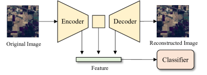
((a))

((b))

Figure 1: Different unsupervised feature learning frameworks including (a) existing unsupervised feature learning and (b) ours proposed Diff-HSI that extract timestep-wise features and construct multi-timestep representations by dynamic fusion for the first time.

As another category of HSI classification methods, [20, 21, 22, 23] is designed to learn spectral-spatial features from HSIs in an unsupervised manner. Typically, these methods leverage an encoder-decoder network trained in an unsupervised manner for HSI reconstruction and extract the spectral-spatial feature from the intermediate feature maps, depicted in Fig. 1(a). Although these methods mine implicit spectral attributes and spatial relations through unsupervised feature learning, the reconstruction networks they designed mainly capture low-level reconstruction features such as texture and edge, lacking high-level features which are necessary for discriminative representations to model the spectral-spatial relations comprehensively [24].

Learning rich representations and modeling the complex spectral-spatial relations from high dimensions are significant and should be considered for HSI classification. Most recently, diffusion models [25, 26, 27] have emerged as new generative models with superior performance in generation and reconstruction tasks, and have started to be explored in other computer vision tasks like semantic segmentation [28, 29, 30]. Diffusion models have the ability in the reconstruction task, so they are well-suited as a framework for unsupervised feature learning. Furthermore, there exist two appealing properties of using diffusion models [31, 32, 33] for unsupervised feature learning of hyperspectral data: 1) diffusion models learn implicit mappings, which have superior representation ability on complex problems via simple expressions and extract both high-level and low-level features from images; 2) the stepwise reverse denoising process of diffusion models are modeled as an iterative optimization process optimized by Langevin dynamics. This process brings a large number of degrees of freedom and tries to predict further information conditioned on the given noise-destructed data at every timestep, leading to better generalization to complex problems. When applying diffusion models to unsupervised feature learning of HSI data, it not only learns both high-level and low-level features but also extracts spectral-spatial features in the dimension of timestep $t$, as shown in Fig. 1(b).

Naturally, it is crucial to explore how to exploit abundant timestep-wise features more effectively and efficiently. On the one hand, the timestep-wise features are diverse and informative and may focus on different information. The shallow timestep-wise features are more informative for fine details, while deeper ones are more concerned about high-level semantics and global information [25, 34]. On the other hand, HSIs from various datasets acquired by different sensors exhibit distinct spectral characteristics, leading to variations in the spectral representation patterns of timestep-wise features extracted from different HSI datasets. Meanwhile, the abundant timestep-wise features pose a challenge in terms of computation overheads. In addition, manually selecting timestep-wise features to characterize spectral-spatial features effectively is struggle. Therefore, a dynamic feature fusion module that adaptively fuses features of different timesteps for different HSI datasets is desired.

In view of these, we propose the unsupervised spectral-spatial feature learning framework based on the diffusion model for HSI classification, named Diff-HSI. More specifically, the proposed framework first pretrain a diffusion model with unlabeled HSI patches for unsupervised feature learning, which is able to automatically learn label-agnostic knowledge and mine the connotation of unlabeled data that reveals the complex spectral-spatial dependencies compared to conventional supervised methods. Then, we extract features from different hierarchies from the pretrained denoising U-Net decoder to construct the timestep-wise feature bank, which contains various informative features from different timestep $t$. To effectively harness the features from the timestep-wise feature bank and softly learn the proper timestep-wise feature combination for different HSI datasets, we propose a dynamic feature fusion module. This module is designed to adaptively fuse hierarchical features from different timesteps, generating multi-timestep representations enriched with comprehensive spectral-spatial information. Ultimately, an ensemble of linear classifiers is employed to leverage these dynamic representations for accurate HSI classification.

To summarize, our contributions are listed as follows.

• As a pioneer work, we introduce diffusion models to HSI classification and propose a diffusion-based unsupervised feature learning framework called Diff-HSI, which can implicitly learn both high-level and low-level features to model complex spectral-spatial relations.

• To leverage abundant timestep-wise features effectively and efficiently, we construct a timestep-wise feature bank with hierarchical features from different timesteps, and design a dynamic feature fusion module to fuse these timestep-wise features adaptively. The above process learns the soft timestep-wise feature combination for each labeled patch of different HSI datasets and constructs comprehensive multi-timestep representations.

• Compared with several state-of-the-art supervised and unsupervised methods, experimental results demonstrate that our proposed method achieves superior classification accuracy on three public HSI datasets.

The remainder of this paper is organized as follows. Section II describes related work. In Section III, our proposed Diff-HSI is introduced in detail. Section IV conducts extensive experiments on three HSI datasets to demonstrate the effectiveness of the proposed method. Finally, some conclusions are drawn in Section V.

II Related Work

II-A Supervised-based HSI Classification Methods

Due to the remarkable breakthroughs achieved by deep learning in various computer vision tasks, many progressive deep learning-based networks have been widely utilized for supervised HSI classification methods, e.g., autoencoders (AEs) [21], deep belief networks (DBNs) [35] and recurrent neural networks (RNNs) [36]. Among these, CNNs draw significant attention with their excellent feature extraction capability and become mainstream in HSI classification [13, 14, 15]. CNNs can effectively extract spectral-spatial features through their ability to extract spatially structural information and locally contextual information. As the vision transformer rises in the field of computer vision, researchers begin to explore the value of the transformer in HSI classification and find it outperforms CNN-based methods in solving the problem of long-term spectral information dependencies [16, 17, 18, 19]. Although these supervised methods have achieved promising performance, they still require large amounts of labeled HSI samples, and are limited to modeling complex relations and capturing label-agnostic information.

II-B Unsupervised-based HSI Classification Methods

Unsupervised feature learning is a feature extraction paradigm to automatically learn feature representations from the input data without any annotated information. Leveraging unsupervised feature learning on unlabeled HSI patches is a solution to the limited labeled samples of HSI datasets. Typically, the commonly used unsupervised feature learning methods in HSI classification are based on the encoder–decoder paradigm, where an autoencoder-like network encodes the input HSI patches into a refined feature and then reconstructs the feature to initial HSI data by a decoder. Mou et al. [20] first design a fully 2D Conv–Deconv network in an end-to-end manner for unsupervised feature learning of HSI classification. Similarly, Mei et al. [21] design a 3D convolutional autoencoder (3D-CAE) for unsupervised feature learning of HSI classification. To alleviate the insufficiency of geometric representation and exploit the multi-scale features, Zhang et al. [22] design a multi-scale CNN-based unsupervised feature learning framework, with two branches of decoder and clustering optimized by the error feedback of image reconstruction and pseudo-label classification. In the aforementioned approaches, the feature representations learned from the unlabeled HSI patches contain more spectral-spatial information than supervised methods; however, they mainly focus on low-level visual concepts and ignore high-level feature extraction for HSI classification, which is solved in our methods.

II-C Diffusion Models

Diffusion models are a class of probabilistic generative models that progressively inject a standard Gaussian noise, then learn a model to reverse this process for sample generation [25, 26, 27]. Current research on diffusion models is mostly based on three formulations: denoising diffusion probabilistic models (DDPMs) [25], score-based generative models [33], and stochastic differential equations [37]. DDPMs are the mainstream diffusion models, and a large number of recent works based on DDPMs have made DDPMs increasingly powerful in terms of generative quality and diversity over other generative models [38]. Meanwhile, DDPMs have been widely used in several applications, including super-resolution [39], inpainting [40], and point cloud generation [41]. However, to the best of our knowledge, few works successfully adopt them to HSI classification. When applying diffusion models to HSI classification, it can not only implicitly learn both high-level and low-level features but also extract spectral-spatial features in the dimension of timestep $t$, leading to improvement in modeling complex spectral-spatial relations.

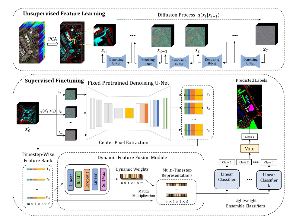
Figure 2: Overview of our proposed Diff-HSI. The method consists of two steps. Step 1: We pretrain the DDPM with HSI patches in an unsupervised manner and then freeze the parameters. Step 2: We construct a timestep-wise feature bank by extracting hierarchical features from the fixed pretrained U-Net decoder in terms of different timestep $t$. In order to softly fuse the features, a dynamic feature fusion module is designed to obtain effective multi-timestep representations adaptively. Finally, an ensemble of lightweight classifiers is trained by leveraging the multi-timestep representations of label-limited HSI patches to perform HSI classification.

III Method

Our proposed Diff-HSI aims to learn effective spectral-spatial representations in an unsupervised manner via denoising diffusion probabilistic model (DDPM) for HSI classification. The framework is shown in Fig. 2. Our method consists of two key steps. The first step is to pretrain the DDPM with unlabeled patches to learn complex spectral-spatial distributions and dependencies of HSI data. After pretraining, we freeze the parameters of the pretrained DDPM. The second step of our Diff-HSI is a supervised learning process aiming to fully extract and dynamically fuse the timestep-wise features from the pretrained denoising U-Net for classification. In order to capture the characteristics of different objects in HSI data, we first extract abundant spectral-spatial features from different timestep $t$ to construct the timestep-wise feature bank. Then, we design a dynamic feature fusion module that fuses the features in the feature bank dynamically and generates multi-timestep representations with discriminative information for classification. Finally, the representations are fed into an ensemble of lightweight classifiers to predict the label of the center pixel. In this section, we introduce our proposed Diff-HSI in detail, including the unsupervised diffusion-based pretraining step as well as the supervised finetuning step with multi-timestep representation generation.

III-A Diffusion-based Unsupervised Spectral-Spatial Feature Learning

In order to learn complex spectral-spatial relations and label-agnostic information of HSI data, we pretrain a diffusion model in an unsupervised manner in the first step of our Diff-HSI. We first give a brief review of DDPM and introduce the basic principles to make our method easier to understand. Then, we explain our unsupervised feature learning procedure in detail through diffusion-based pretraining with HSI data.

III-A1 A Brief Review of DDPM

Denoising diffusion probabilistic models are a class of likelihood-based models that reconstruct the distribution of training data via an encoder-decoder denoising model. The denoising model is trained to remove noise from the training data destructed by Gaussian noises step-by-step. These models consist of a forward noising process and a reverse denoising process. In the forward process, Gaussian noise is added to the original training data $x_{0}\sim q\left(x_{0}\right)$ step by step over $T$ time steps, which follows the Markovian process:

$$q(x_{t}|x_{t-1})=\mathcal{N}(\sqrt{1-\beta_{t}}x_{t-1},\beta_{t}I)$$ (1)

where $\mathcal{N}(.)$ is a Gaussian distribution, and the Gaussian variances $\{\beta_{t}\}_{t=0}^{T}$ that determines the noise schedule are either be learned or scheduled. The above formulation leads that an arbitrary noisy sample $x_{t}$ for each timestep $t$ is obtained directly from $x_{0}$:

$$x_{t}=\sqrt{\overline{\alpha}_{t}}x_{0}+\sqrt{(1-\overline{\alpha}_{t})}\epsilon,\epsilon\sim\mathcal{N}(0,I)$$ (2)

where $\alpha_{t}=1-\beta_{t}$, and $\overline{\alpha}_{t}=\prod_{s=1}^{t}\alpha_{s}$. Then in the reverse process, DDPM also follows a Markovian process to denoise the noisy sample $x_{T}$ to $x_{0}$ step by step. Under large $T$ and small $\beta_{t}$, the reverse transitions probability is approximated as a Gaussian distribution and is predicted by a learned neural network as follows:

$$p_{\theta}(x_{t-1}|x_{t})=\mathcal{N}(x_{t-1};\mu_{\theta}(x_{t},t),\sigma_{\theta}(x_{t},t))$$ (3)

where the reverse process is re-parameterized by estimating $\mu_{\theta}(x_{t},t)$ and $\sigma_{\theta}(x_{t},t)$. $\sigma_{\theta}(x_{t},t)$ is set to $\sigma_{t}^{2}\mathbf{I}$, where $\sigma_{t}^{2}$ is not learned. In practice, rather than predicting $\mu_{\theta}(x_{t},t)$ directly, predicting the noise $\epsilon$ in Eq. 2 via a U-Net works best, and the parameterization of $\mu_{\theta}(x_{t},t)$ is derived as follows:

$$\mu_{\theta}(x_{t},t)=\frac{1}{\sqrt{\alpha_{t}}}(x_{t}-\frac{1-\alpha_{t}}{\sqrt{1-\overline{\alpha}_{t}}}\epsilon_{\theta}(x_{t},t))$$ (4)

The U-Net denoising model $\epsilon_{\theta}(x_{t},t)$ is optimized by minimizing the following loss function:

$$\mathcal{L}(\theta)=E_{t,x_{0},\epsilon}[(\epsilon-\epsilon_{\theta}(\sqrt{\overline{\alpha}_{t}}x_{0})+\sqrt{1-\overline{\alpha}_{t}\epsilon},t)^{2}]$$ (5)

In our work, improved DDPM [27] is adopted and has been proven to bring some improvements to the above DDPM. In detail, learned variances $\sigma_{\theta}(x_{t},t)$ and an improved cosine noise schedule proposed in [27] lead to enhanced distribution learning ability.

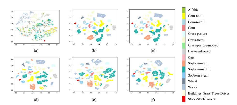
Figure 3: 2D t-SNE visualization of features from different timesteps on the Indian Pines dataset. (a) original spectral feature. (b) feature at $t=100$. (c) feature at $t=300$. (d) feature at $t=500$. (e) feature at $t=700$. (f) feature at $t=900$.

III-A2 Unsupervised Hyperspectral Diffusion Pretraining

Using the training skills and optimization objectives mentioned above, our DDPM is trained by unlabeled hyperspectral data. Suppose that $S$ is the set of all samples in a dataset, $D$ is a denoising diffusion probabilistic model, and $E$ is an ensemble of lightweight classifiers. The target of the unsupervised pretraining step is to learn label-agnostic spectral-spatial features on unlabelled data sampled from $S$ so that the features can be leveraged in the finetuning step to train ensemble lightweight classifiers using a small amount of labeled data sampled from $S_{labeled}\in S$ for classification.

In order to learn effective spectral-spatial features in an unsupervised manner, we first pretrain a denoising diffusion probabilistic model with unlabeled patches randomly cropped from the HSI dataset. Before training, the data is pre-processed by principal components analysis (PCA) and patch cropping operation. Then, patches are randomly sampled from compressed HSI for DDPM pretraining. In detail, given an unlabeled patch $x_{0}\in\mathcal{R}^{H\times H}$, we gradually add Gaussian noise to the HSI patch according to the variance schedule $\{\beta_{t}\}_{t=0}^{T}$ in the diffusion process where $T$ is the total number of the timestep. Then, in the reverse process, a denoising U-Net is trained to predict the noise added on $x_{t-1}$ taking noisy patch $x_{t}$ and timestep $t$ as inputs. And $x_{t-1}$ is calculated by subtracting the predicted noise from $x_{t}$. In other words, the model tries to capture some useful information of $x_{t}$ to reconstruct $x_{t-1}$ that is closer to $x_{0}$. In each step of the training process, the timestep $t$ is randomly sampled from 0 to $T$.

In the pretraining procedure with unlabeled hyperspectral data, the DDPM is able to automatically learn the label-agnostic prior of HSI data that reveals the complex dependencies and relations in the spectral and spatial dimensions. At different timesteps, different input noisy patches and their optimization goals allow the DDPM to attend to varied information of the data, which is demonstrated to be critical to HSI classification.

III-B Multi-Timestep Representation for Supervised Finetuning

After unsupervised pretraining, in order to explore the rich information learned by the pretrained DDPM, the second step of our method is to extract effective features from the pretrained DDPM and construct multi-timestep representations for HSI classification. We first extract abundant features and construct a timestep-wise feature bank. Then, a dynamic feature fusion module is designed to automatically fuse the features into multi-timestep representations. Finally, ensemble lightweight classifiers are trained for classification.

III-B1 Timestep-Wise Feature Bank

In the finetuning step, the parameters of the pretrained DDPM are frozen. The denoising U-Net is able to capture meaningful information from the input data in the reverse process. Leveraging the rich and diverse information captured in the reverse steps is crucial for accurate classification. Therefore, timestep-wise spectral-spatial features are extracted from the intermediate hierarchies of DDPM at different timesteps to construct effective representations that contain diverse information of input HSI. Given an input patch $x_{0}\in\mathcal{R}^{H\times H}$ randomly cropped from HSI and a timestep $t$, Gaussian noise is gradually added to $x_{0}$ according to the variance schedule through diffusion process $q(x_{t}|x_{0})$. The noisy patch $x_{t}$ can be directly obtained by equation 2. Then, the noisy patch $x_{t}$ is fed into the pretrained denoising U-Net to obtain hierarchal features from the U-Net decoder, which implies rich spectral information as well as multi-scale spatial information, as shown in Fig. 2. The features from different layers of the decoder are jointly upsampled to $H\times H$ and then concatenated to get the feature $f_{t}\in\mathcal{R}^{H\times H\times d}$ at timestep $t$. The above process is defined as a function $\mathcal{F}$ and formulated as follows:

$$f_{t}=\mathcal{F}(D,x_{t},t)$$ (6)

where $D$ is the pretrained denoising U-Net.

For each feature $f_{t_{i}}\in\mathcal{R}^{H\times H\times d}$, we reserve only the vector corresponding to the center pixel indexed as $(\frac{H}{2},\frac{H}{2})$ to obtain the pixel-wise feature $h_{t_{i}}\in\mathcal{R}^{1\times 1\times d}$, which largely reduce computational cost with fewer parameters. Following the above process, we draw $m$ sets of features to construct the timestep-wise feature bank:

$$\mathcal{B}=\{h_{t_{i}}|i\in\{1,...,m\},h_{t_{i}}=center(f_{t_{i}})\}$$ (7)

where $t_{1},...,t_{m}$ are sampled from $[0,T]$ at equal intervals. Features extracted at different timestep $t$ tend to capture different information of HSI data since the reverse process is a step-by-step denoising process that tries to predict further information conditioned on the given destructed data at every different timestep.

To further demonstrate this, we visualize the features in 2-dimensional space using t-distributed stochastic neighbor embedding (TSNE) to show the diversity of features at different timesteps $t$. The visualization of the original spectral feature space is shown in Fig. 3(a), and the features in the timestep-wise feature bank at timestep 100, 300, 500, 700, and 900 are visualized in Fig. 3(b)-(f) respectively. As observed, the features in the timestep-wise feature bank show great diversity. Furthermore, with the increase of timestep $t$, the clusters of the features tend to be more loosely structured, and features of the same class tend to be formed into a few large clusters rather than dispersed into multiple smaller clusters. Features at smaller $t$ tend to capture stochastic variation, and features at larger $t$ tend to focus on high-level information, both of which are key to HSI classification with different categories of land covers. Thus the abundant features in the feature bank contain diverse and multi-level information of the input HSI data, exhibiting diverse properties and concerns.

III-B2 Dynamic Feature Fusion Module

For each input HSI patch $x_{0}$, a timestep-wise feature bank is obtained with abundant features containing varied characteristics of the patch. However, the features contain a wealth of information, but not all of it is essential. Using all the features for classification will bring high computational costs and redundant information, and manually selecting timestep-wise features from the feature bank is difficult to characterize spectral-spatial features effectively and robustly. Meanwhile, HSI data have different spectral characteristics for different HSI datasets, resulting in different spectral representation laws of timestep-wise features. Also, data on the same dataset is very different due to its position. Therefore, the dynamic feature fusion module is crucial to be proposed, and is capable of adaptively fusing features of different timesteps from the DDPM to learn effective multi-timestep representations with key information.

To obtain dynamic multi-timestep representations, we design the dynamic feature fusion module to predict the soft dynamic weight of multi-timestep representations. The architecture of the dynamic feature fusion module is illustrated in Fig. 2. Specifically, Let $L=[h_{t_{1}}...h_{t_{m}}]$ denotes the concatenated features from the timestep-wise feature bank as the input of the dynamic weight network. The dynamic weight network consists of two linear layers and outputs the $n$ sets of dynamic weights $w$ with a SoftMax function:

$$w =\mathcal{M}(L,W)=SoftMax(a(L,W))$$ (8)

$$=SoftMax(W_{2}\delta(W_{1}L))$$

where $M$ is the dynamic weight network, $W$ is the linear weight of $M$, $\delta$ is ReLU function, $w\in\mathcal{R}^{m\times 1\times 1\times n}$ and $L\in\mathcal{R}^{m\times 1\times 1\times n}$. Inspired by the design of the multi-head attention mechanism in [42], we generate multiple sets of dynamic weights, which allows the representations to focus on different information from different positions and spectral bands. Each dynamic weight determines the proportion of each feature in the corresponding representation. Then, the dynamic weights are used to weight the pixel-wise features by matrix multiplication to obtain $n$ multi-timestep representations:

$$r_{i}=w^{T}_{i}L$$ (9)

where $r_{i}$ is the i-th representation, $i\in{1,...,n}$. The multi-step representations will be concatenated into the final representation to be classified. Thus, the most appropriate and relevant representation is automatically learned from the feature bank without human intervention, saving time cost and reducing the impact of redundant information. $n$ will be ablated to find the most suitable value balancing the performance and computational cost.

III-B3 Lightweight Ensemble Classifiers

After getting the dynamic representation, a lightweight network is needed to predict the classification label. Inspired by [43], we train an ensemble of lightweight linear classifiers that takes the dynamic pixel representations as inputs and predicts the classification label of each pixel. Specifically, each classifier is trained independently, consisting of two hidden layers with ReLU activation and batch normalization. When testing a sample, the final predicted label is obtained by majority voting of the ensemble of pixel classifiers, as illustrated in Fig. 2. This method brings more stability of prediction with a very small cost since the parameters of each classifier are very limited.

IV Experiments and results

In this section, we first describe the three used well-known HSI datasets, including the Indian Pines dataset, Pavia University dataset and Houston2018 dataset. The experimental setting is then introduced including evaluation metrics, a brief introduction of compared state-of-art methods, and implementation details. Then, we conduct quantitative experiments and ablation analysis to evaluate our proposed method.

IV-A Datasets Description

IV-A1 Indian Pines

The Indian Pines dataset was acquired in 1992 over an area of Indian pines in North-Western Indiana by Airborne Visible Infrared Imaging Spectrometer (AVIRIS) sensor. It consists of $145\times 145$ pixels with a spatial resolution of 20 m and 220 spectral bands in the wavelength range of 400 to 2500 nm. There are 200 bands retained for classification (1-103, 109-149, 164-219) after removing the bands affected by noise. The dataset contains 10249 labeled pixels with 16 categories. We use 10% of the labeled samples for training and the rest for testing. The class name and the number of training and testing samples are listed in Table I.

IV-A2 Pavia University

The University of Pavia dataset was collected in 2003 by the reflective optics system imaging spectrometer (ROSIS-3) sensor over a part of the city of Pavia, Italy. The dataset consists of $610\times 340$ pixels with a spatial resolution of 1.3 m and 115 spectral bands in the wavelength range of 430 to 860 nm. 103 out of 115 bands are used for classification after removing 12 noisy bands. The image contains a large number of background pixels and only 42776 labeled pixels divided into 9 classes, including asphalt, meadows, gravel, and so on. We use 5% of the labeled samples for training and the rest for testing. The class name and the number of training and testing samples are listed in Table II.

IV-A3 Houston2018

The Houston2018 dataset, identified as 2018 IEEE GRSS DFC dataset, was gathered in 2018 by the National Center for Airborne Laser Mapping (NCALM) over the University of Houston campus and its neighboring urban area, including HSI, multispectral LiDAR, and very high resolution RGB images. The HSI dataset consists of $601\times 2384$ pixels with a spatial resolution of 1 m and 48 spectral bands in the wavelength range of 380 to 1050 nm. It contains 504856 labeled pixels and 20 classes of interest. We use 5% of the labeled samples for training and the rest for testing. The class name and the number of training and testing samples are listed in Table III.

TABLE I: Land-cover types, the number of labeled training samples and testing samples of the Indian Pines dataset.

Class	Land Cover Type	Training	Testing
1	Alfalfa	5	41
2	Corn-Notill	143	1285
3	Corn-Mintill	83	747
4	Corn	24	213
5	Grass-Pasture	48	435
6	Grass-Trees	73	657
7	Grass-Pasture-Mowed	3	25
8	Hay-Windrowed	48	430
9	Oats	2	18
10	Soybean-Notill	97	875
11	Soybean-Mintill	245	2210
12	Soybean-Clean	59	534
13	Wheat	20	185
14	Woods	126	1139
15	Buildings-Grass-Trees-Drives	39	347
16	Stone-Steel-Towers	9	84
	Total	1024	9225

TABLE II: Land-cover types, the number of labeled training samples and testing samples of the Pavia University dataset.

Class	Land Cover Type	Training	Testing
1	Asphalt	332	6299
2	Meadows	932	17717
3	Gravel	105	1994
4	Trees	153	2911
5	Painted Metal Sheets	67	1278
6	Bare Soil	251	4778
7	Bitumen	67	1263
8	Self-Blocking Bricks	184	3498
9	Shadows	47	900
	Total	2138	40638

TABLE III: Land-cover types, the number of labeled training samples and testing samples of the Houston2018 dataset.

Class	Land Cover Type	Training	Testing
1	Healthy Grass	490	9309
2	Stressed Grass	1625	30877
3	Artificial turf	34	650
4	Evergreen trees	680	12915
5	Deciduous trees	251	4770
6	Bare earth	226	4290
7	Water	13	253
8	Residential buildings	1989	37783
9	Non-residential buildings	11187	212565
10	Roads	2293	43573
11	Sidewalks	1702	32327
12	Crosswalks	76	1442
13	Major thoroughfares	2317	44031
14	Highways	493	9372
15	Railways	347	6590
16	Paved parking lots	575	10925
17	Unpaved parking lots	7	139
18	Cars	327	6220
19	Trains	269	5100
20	Stadium seats	341	6483
	Total	25242	479614

TABLE IV: Quantitative performance of different classification methods in terms of OA, AA, and $\kappa$ as well as the accuracies for each class on the Indian Pines dataset. The best one is shown in bold.

Class	CNN Based Methods			Transformer Based Methods			Unsupervised Methods		Diff-HSI
	2-D CNN	3-D CNN	SSRN	SF	SSFTT	GAHT	3DCAE	UMSDFL
1	65.85	58.54	94.14	63.00	95.12	97.56	72.97	99.10	99.51
2	99.77	76.19	97.84	92.35	97.67	98.05	88.50	96.10	98.89
3	81.66	77.64	97.54	86.86	98.87	98.66	87.20	95.39	99.84
4	96.71	52.11	90.70	88.96	91.55	95.31	84.90	97.24	99.81
5	85.75	93.56	97.75	92.49	96.32	95.17	90.28	94.12	98.85
6	97.87	98.17	99.24	99.12	99.54	99.85	97.97	99.25	100.00
7	100.00	36.00	81.60	52.50	100.00	100.00	56.52	88.46	98.40
8	100.00	98.60	100.00	99.16	100.00	100.00	99.48	100.00	100.00
9	50.00	55.56	74.44	41.18	88.89	100.00	87.50	94.44	100.00
10	35.54	82.86	94.77	93.16	97.71	94.29	86.80	95.84	98.88
11	88.01	90.45	98.87	92.27	98.69	99.37	96.68	99.29	99.63
12	98.13	62.55	97.83	85.44	98.13	96.63	80.83	93.37	98.91
13	99.46	88.65	99.24	99.02	97.28	100.00	100.00	100.00	99.89
14	99.91	99.39	99.18	96.73	99.91	97.89	99.90	95.25	100.00
15	91.35	86.17	93.95	83.41	98.84	97.12	96.80	99.15	99.25
16	86.90	45.24	98.33	93.50	95.54	94.05	84.00	100.00	98.10
OA (%)	87.77	85.42	97.75	92.31	97.47	97.95	92.69	97.02	99.46
AA (%)	86.06	75.10	94.71	84.95	96.57	97.75	88.15	96.00	99.37
$\kappa$	0.8603	0.8324	0.9743	0.9124	0.9711	0.9766	0.9162	0.9660	0.9938

TABLE V: Quantitative performance of different classification methods in terms of OA, AA, and $\kappa$, as well as the accuracies for each class on the Pavia University dataset. The best one is shown in bold.

Class	CNN Based Methods			Transformer Based Methods			Unsupervised Methods		Diff-HSI
	2-D CNN	3-D CNN	SSRN	SF	SSFTT	GAHT	3DCAE	UMSDFL
1	99.68	97.02	98.81	96.21	99.33	99.38	94.20	99.62	100.00
2	99.41	99.97	99.83	99.64	99.92	99.80	99.58	99.98	99.99
3	86.56	92.98	92.45	87.65	98.29	98.35	78.83	91.02	100.00
4	98.18	97.53	98.32	96.64	98.49	99.52	97.53	98.40	99.51
5	99.84	99.06	99.65	99.97	99.53	100.00	100.00	100.00	100.00
6	100.00	99.10	99.43	99.56	100.00	99.75	95.30	98.32	100.00
7	99.84	79.10	99.76	90.30	99.13	99.60	97.42	99.61	100.00
8	100.00	97.34	99.32	94.60	98.05	98.63	96.87	98.36	99.82
9	98.22	95.22	99.82	98.49	95.44	99.33	98.61	99.89	99.96
OA (%)	98.86	97.88	99.10	97.54	99.21	99.53	96.77	99.02	99.94
AA (%)	97.97	95.26	98.60	95.88	98.69	99.37	95.37	98.36	99.92
$\kappa$	0.9848	0.9719	0.9881	0.9674	0.9915	0.9937	0.9571	0.9870	0.9993

TABLE VI: Quantitative performance of different classification methods in terms of OA, AA, and $\kappa$ as well as the accuracies for each class on the Houston2018 dataset. The best one is shown in bold.

Class	CNN Based Methods			Transformer Based Methods			Unsupervised Methods		Diff-HSI
	2-D CNN	3-D CNN	SSRN	SF	SSFTT	GAHT	3DCAE	UMSDFL
1	84.33	82.02	86.30	92.36	79.93	79.50	91.60	88.99	89.41
2	95.98	96.64	95.32	95.08	93.44	96.55	93.92	97.53	96.24
3	96.92	96.00	99.72	96.21	99.66	100.00	97.60	99.23	99.88
4	98.13	95.55	97.49	98.48	96.64	97.62	95.92	97.98	99.26
5	91.26	79.16	86.09	91.87	90.11	95.01	85.79	92.51	96.86
6	99.91	97.51	98.48	99.62	99.62	99.91	98.50	99.58	100.00
7	80.63	71.94	93.68	27.01	85.45	95.65	61.15	96.85	97.63
8	94.29	88.62	91.62	95.42	98.72	99.18	91.15	94.20	99.62
9	99.54	92.80	97.88	98.60	99.09	99.35	95.12	99.07	99.63
10	95.44	71.61	81.72	88.22	91.15	92.64	76.72	88.61	95.89
11	77.86	73.17	69.44	27.01	80.97	85.73	70.22	82.28	93.02
12	15.26	11.10	0.51	31.46	41.69	33.43	4.79	42.76	50.23
13	87.30	69.12	84.59	91.79	94.49	96.79	90.52	93.26	97.72
14	94.97	96.18	89.65	92.91	96.97	99.17	87.23	97.02	99.23
15	95.40	98.98	99.34	99.33	99.30	99.92	99.06	99.59	99.81
16	93.62	90.40	91.00	96.36	97.84	98.15	92.01	96.36	99.69
17	86.33	20.86	0.00	22.78	69.21	90.65	0.00	100.00	94.10
18	96.64	89.05	93.66	91.61	93.07	97.85	90.43	94.24	99.46
19	99.24	95.45	96.92	96.53	97.97	99.84	96.09	99.59	99.89
20	92.77	93.92	99.12	99.77	99.96	100.00	97.27	99.89	99.94
OA (%)	94.84	86.88	91.61	90.65	95.48	96.69	90.34	95.38	98.07
AA (%)	88.79	80.50	82.63	80.75	90.26	92.85	80.76	92.98	95.37
$\kappa$	0.9325	0.8313	0.8906	0.8784	0.9412	0.9570	0.8751	0.9398	0.9748

IV-B Experimental Setting

IV-B1 Evaluation Metrics

We evaluate the performance of all methods by three widely used indexes: overall accuracy (OA), average accuracy (AA), and Kappa coefficient ($\kappa$).

IV-B2 Comparison with State-of-the-art Methods

To demonstrate the effectiveness of our proposed method, we compare our classification performance with several state-of-the-art approaches, including CNN-based and transformer-based supervised methods, and unsupervised methods. We use the most effective setting for each of these methods.

• The 2-D CNN architecture contains three 2-D convolution blocks and a softmax layer. Each convolution block consists of a 2-D convolution layer, a BN layer, an avg-pooling layer, and a ReLU activation function.

• The 3-D CNN contains three 3-D convolution blocks and a softmax layer. Each 3-D convolution block consists of a 3-D convolution layer, a BN layer, a ReLU activation function, and a 3-D convolution layer with step size 2.

• The SSRN[14] is a spectral-spatial residual network based on 3-D CNN and residual connection. Spatial residual blocks and spatial residual blocks are designed to extract discriminative features from HSI data.

• For SF[16], there are four encoder blocks in the ViT-based network. In the transformer framework of SF, group-wise spectral embedding and cross-layer adaptive fusion modules are adopted to capture local spectral representations from neighboring bands.

• The SSFTT[17] systematically combines CNN network and transformer structure to exploit spectral-spatial information in the HSI, with a Gaussian weighted feature tokenizer module making the samples more separable.

• The GAHT[18] is a end-to-end group-aware transformer method with three-stage hierarchical framework.

• The 3DCAE[21] is an unsupervised method using the encoder-decoder backbone with 3D convolution operation to learn spectral-spatial features.

• The UMSDFL[22] is an unsupervised method using encoder and decoder with convolutional layers to learn spectral-spatial features. A clustering branch and a multi-layer fusion module is designed to enhance the features.

IV-B3 Implementation Details

The proposed Diff-HSI was implemented using the Pytorch framework. The patch size is set to $48\times 48$, and the dimension of PCA is set to 10. In the diffusion-pretraining procedure, we use Kullback-Leibler Divergence Loss as the loss function. And the Adam optimizer is adopted with a batch size of 128 and a learning rate of 1e-4. In the second stage, the cross-entropy loss is used in lightweight classifiers. $m$, $n$, and $k$ are set to be 20, 3, and 5, respectively. We adopt the Adam Optimizer and the Cosine Annealing as our training schedule. The original learning rate and minimum learning rate are set to be 1e-4 and 5e-6, respectively. The number of epochs is set to 100 for all datasets. Fairly, we calculate the results by averaging the results of ten repeated experiments with different training sample selections.

IV-C Quantitative Results and Analysis

Quantitative classification results in terms of class-specific accuracy, OA, AA, and $\kappa$ of the compared methods on the Indian Pines, PaviaU, and Houston 2018 datasets are listed in Table IV, V, and VI, respectively. And the classification maps of all methods are shown in Fig. 4, 5 and 6.

Compared with other methods, our proposed Diff-HSI achieves the highest OA, AA, and $\kappa$ on the three datasets. According to the results, the CNN-based supervised methods obtain good performance owing to the ability of capturing local spatial information. Besides, since transformers are capable of capturing sequential information, transformer-based supervised methods also achieve competitive performance. The GAHT method achieves the best results in CNN-based and transformer-based supervised methods because it balances the local information and the global dependencies. However, the methods that learn explicit mappings have bottlenecks in learning label-agnostic information and complex relations, which limits performance. Some unsupervised methods are proposed to tackle the problem by learning representative features through an encoder-decoder network. Limited by the model architecture, the features learned are not discriminative and rich enough for HSI classification lacking high-level information. Therefore, the performance of these methods is even lower than that of some explicit learning methods. Our proposed Diff-HSI introduces the diffusion model to HSI classification, which has the powerful ability to model complex relations. Furthermore, the features learned by our method are of great diversity, enriching the representation capability. Thus, our Diff-HSI outperforms all the previous methods on the three datasets. Notably, the classification performance of the Houston2018 Dataset is largely improved compared with the previous SOTA method in terms of OA (98.07% versus 96.69%), AA (95.37% versus 92.98%), and $\kappa$ (0.9748 versus 0.9570), which especially demonstrate our effectiveness.

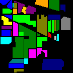
((a))

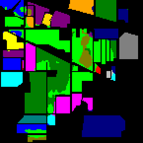
((b))

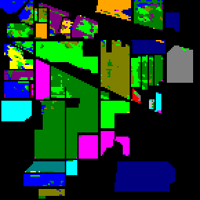
((c))

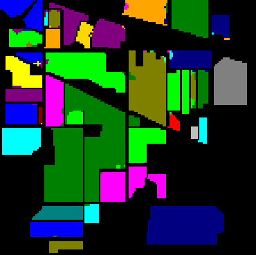
((d))

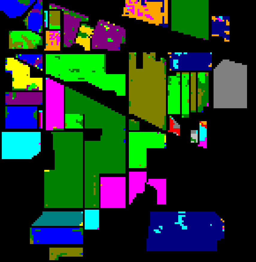
((e))

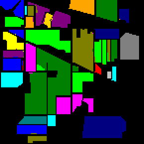
((f))

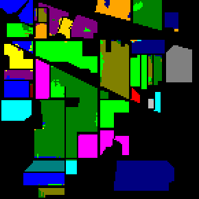
((g))

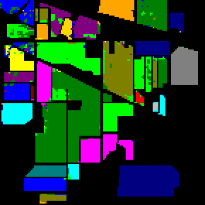
((h))

((i))

((j))

Figure 4: Classification maps obtained by different methods on the Indian Pines dataset. (a) Ground truth. (b) 2-D CNN (OA=87.77%). (c) 3-D CNN (OA=85.42%). (d) SSRN (OA=97.75%). (e) SF (OA=92.31%). (f) SSFTT (OA=97.47%). (g) GAHT (OA=97.95%). (h) 3DCAE (OA=92.69%). (i) UMSDFL (OA=97.02%). (j) Diff-HSI (OA=99.46%).

((a))

((b))

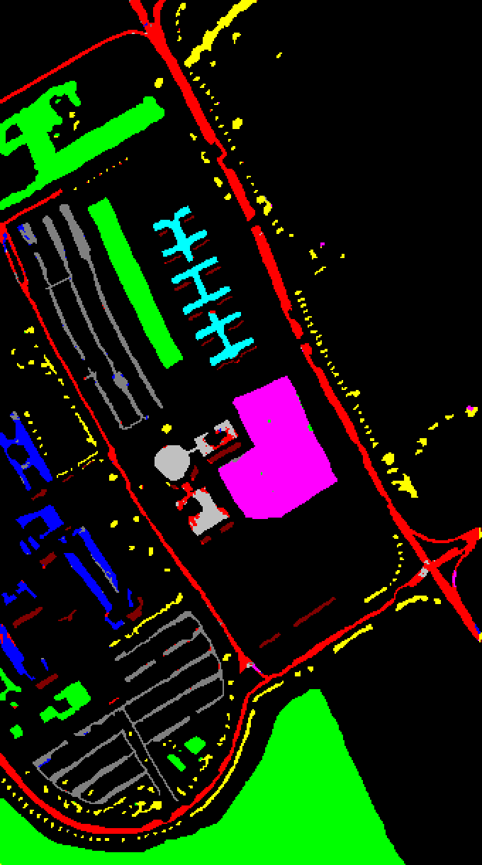
((c))

((d))

((e))

((f))

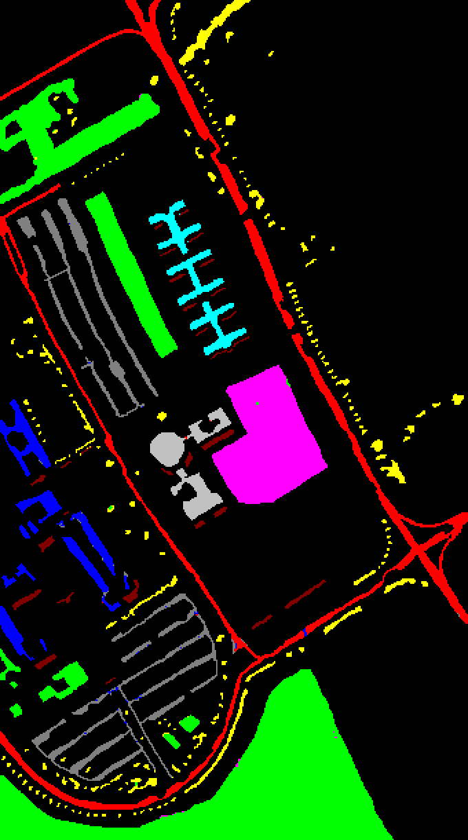
((g))

((h))

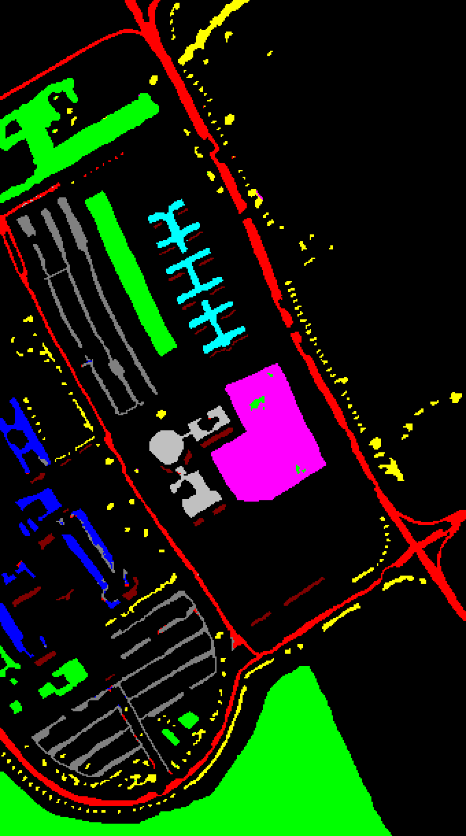
((i))

((j))

Figure 5: Classification maps obtained by different methods on the Pavia University dataset. (a) Ground truth. (b) 2-D CNN (OA=98.86%). (c) 3-D CNN (OA=97.88%). (d) SSRN (OA=99.10%). (e) SF (OA=97.54%). (f) SSFTT (OA=99.21%). (g) GAHT (OA=99.53%). (h) 3DCAE (OA=96.77%). (i) UMSDFL (OA=99.02%). (j) Diff-HSI (OA=99.94%).

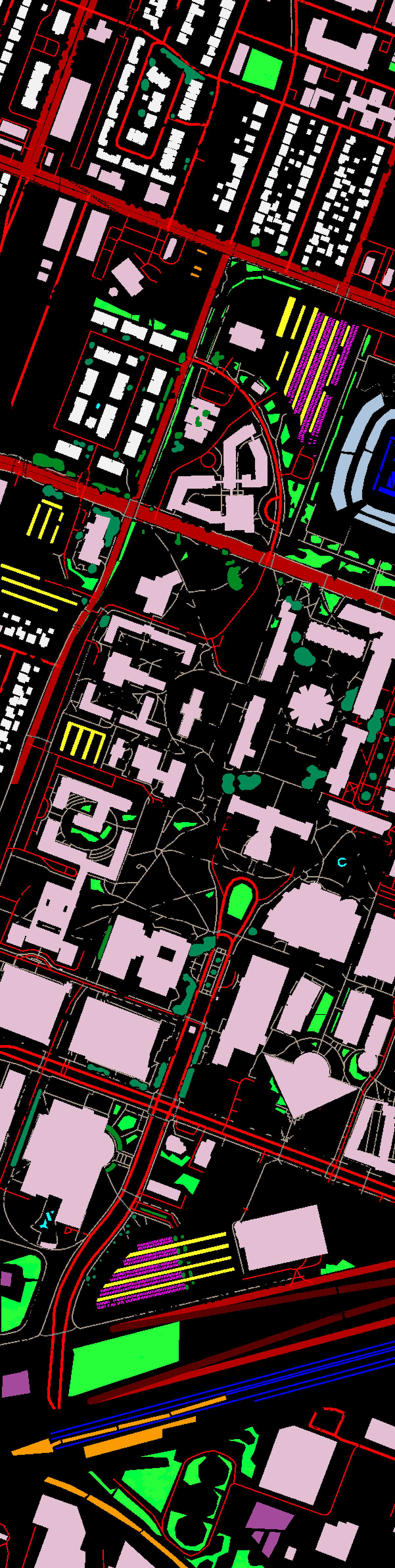
((a))

((b))

((c))

((d))

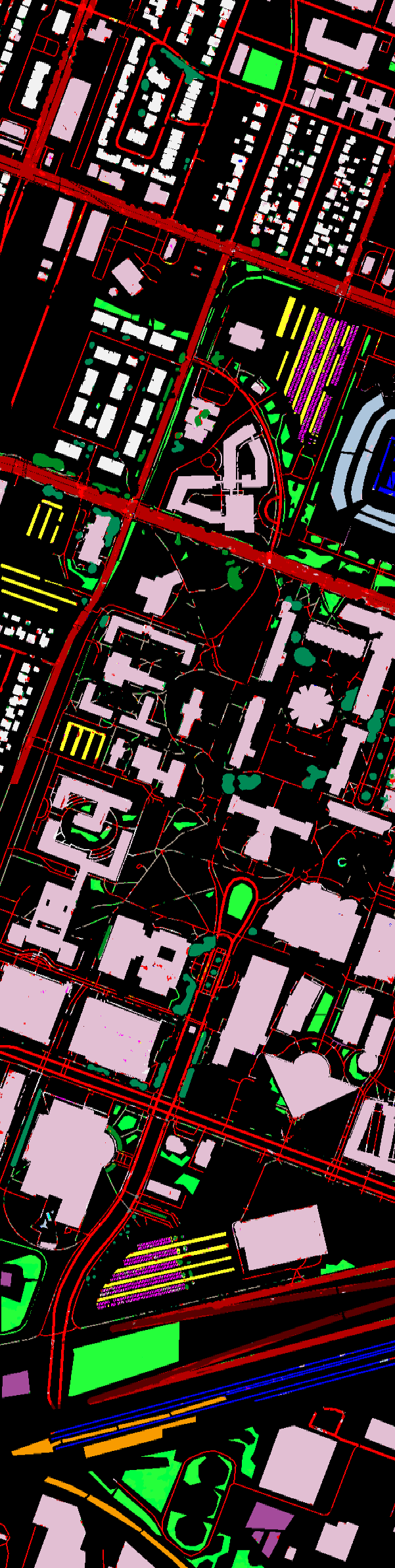
((e))

((f))

((g))

((h))

((i))

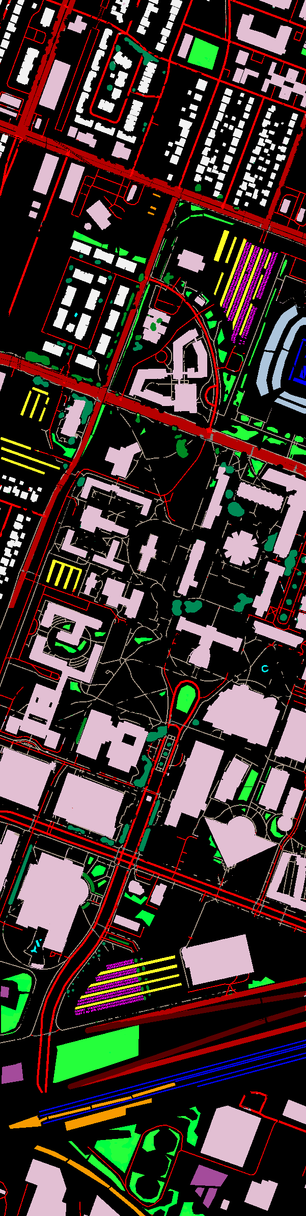
((j))

Figure 6: Classification maps obtained by different methods on the Houston2018 dataset. (a) Ground truth. (b) 2-D CNN (OA=94.84%). (c) 3-D CNN (OA=86.88%). (d) SSRN (OA=91.61%). (e) SF (OA=90.65%). (f) SSFTT (OA=95.48%). (g) GAHT (OA=96.69%). (h) 3DCAE (OA=90.34%). (i) UMSDFL (OA=95.38%). (j) Diff-HSI (OA=98.07%).

IV-D Ablation Studies

In this section, we analyze the effect of the components in our method.

IV-D1 Ablation for Set Number of Dynamic Weights

Our dynamic feature fusion module contains $n$ sets of dynamic weights which impact the classification performance. The change of results by changing $n$ is shown in Tabel VII. We reveal that the best performance is achieved when $n$ is taken as 3. With smaller $n$, only part of the useful information is obtained from the feature bank, which is insufficient for classification. On the other hand, larger $n$ will bring more parameters and excess information.

IV-D2 Ablation for Pretraining Steps

We validate the effectiveness of pretraining on the Indian Pines dataset in terms of OA, AA, and $\kappa$. As shown in Table VIII, only 10k steps pretraining brings dramatic improvement (more than 30% OA) to the final classification performance. Furthermore, as the pretraining steps increase, the performance continues to rise to the best at around 40k steps.

IV-D3 Sensitivity Analysis of Timestep T

To analyze the features extracted from different timestep $t$, we record the change of the classification performance when changing $t$. For easy understanding, we choose 4 of the 16 classes to show their changes, as illustrated in Fig. 7. The performance for each class behaves differently as the $t$ increases. Features of larger $t$ are more sensitive to class ”corn-notill” and features of smaller $t$ are more informative to class ”woods”. For class ”Grass-pasture-mowed” and class ”corn”, features extracted at the intermediate $t$ is the most discriminative. Thus, an appropriate set of $t$ is vital for accurate performance.

TABLE VII: Ablation analysis of the proposed dynamic feature fusion module with a different number of dynamic weight sets in terms of OA, AA, and $\kappa$ on the Indian Pines dataset.

Metric	The number of the sets of dynamic weights $n$
	1	2	3	4
OA (%)	99.36	99.38	99.46	99.43
AA (%)	99.20	99.20	99.37	99.28
$\kappa$	0.9918	0.9930	0.9938	0.9935

TABLE VIII: Effect of Pretraining Steps in terms of OA, AA, and $\kappa$ on the Indian Pines dataset.

Metric	The number of pretraining steps
	0	10k	20k	30k	40k	50k
OA (%)	68.04	97.53	98.40	99.39	99.46	99.45
AA (%)	48.95	96.64	97.76	99.30	99.37	99.39
$\kappa$	58.51	0.9718	0.9817	0.9930	0.9938	0.9936

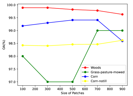
Figure 7: Variation of classification results for four classes with the change of timestep on the Indian Pines dataset.

TABLE IX: Classification performance with different sets of timestep $t$ on the Indian Pines dataset.

Timestep Sets $X$	Metric
	OA (%)	AA (%)	$\kappa$
$[100,200,300]$	98.81	98.72	0.9874
$[700,800,900]$	98.77	98.68	0.9872
$[100,500,900]$	98.87	98.83	0.9886
Dynamic Feature Fusion	99.46	99.37	0.9938

Table IX shows the results with several sets of manually assigned $t$. Specifically, given a timestep set $X=[t_{1},t_{2},t_{3}]$, we extract the features at timestep $t_{1}$, $t_{2}$, and $t_{3}$ to construct the pixel-wise representation for classification. As Table IX presents, the performance is sensitive to the choice of $t$. $X$ with a large $t$, a small $t$ and a medial $t$ performs better than $X$ with only smaller $t$ or larger $t$. Because the former contains a wider range of $t$ leading to more diverse features which make the representation more general for samples of all classes. However, representation obtained by the manually designed method is not always the most appropriate for each sample, since it sacrifices some specificity to improve generalization. So we propose the dynamic feature fusion module to customize $T$ for each sample which makes it more accurate for classification. The results in Table IX demonstrate that our dynamic feature fusion module learns more effective representation compared with the manually selected method.

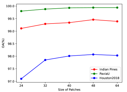
Figure 8: Classification results of different patch sizes on the Indian Pines, Pavia University, and Houston2018 Dataset.

Figure 9: Classification results of different PCA components on the Indian Pines, Pavia University, and Houston2018 Dataset.

IV-E Parameter Analysis

In this section, we analyze the effect of various parameters that influence classification performance by training our proposed Diff-HSI in the same experimental setting as Section IV-B with different parameters.

IV-E1 Effect of Different Patch Size

First, we discuss the effect of different patch sizes on classification performance by two indexes, OA and AA. As shown in Fig. 8, the patch size varies from 24$\times$24 to 60$\times$60. as the patch size increases, the performance first increases and then decreases. The best performance is obtained when the patch size is 48$\times$48 with OA of 99.39% and AA of 99.30%. Too small patches contain insufficient spatial information and too large patches reduce the attention to detailed structures. Thus, we choose 48$\times$48 to be the patch size for the proposed Diff-HSI.

IV-E2 Effect of Different PCA Components

This section analyzes the influence of the number of PCA components, which determines how much spectral information is retained in the compressed data. As the number of PCA components increases, more spectral information is retained while more computational cost and more redundant information are brought. Since each dataset has a different number of channels, the range of PCA components is different for the three datasets. Assuming that $N$ is the channel number of a dataset, the number of PCA components varies from $N/20$ to $N/5$. According to the results shown in Fig. 9, the best performance is achieved at PCA components of $N/8$.

V Conclusion

HSI contains rich spectral-spatial information and complex relations, which are critical for classification tasks. We propose the Diff-HSI method to learn discriminative spectral-spatial features in an unsupervised manner using the diffusion model. Most of the existing works perform HSI classification in an explicit way based on CNN or Transformer. These methods often heavily rely on the number of labeled data and are insufficient to model complex relations, limiting the improvement in performance. Some works explore unsupervised learning for HSI classification through an encoder-decoder feature learning method. However, limited by the feature-extracting capability of the model, they mainly tend to capture low-level features, lacking high-level features which are significant for discriminative spectral-spatial feature representation. Our proposed method leverages the powerful implicit learning ability of the diffusion model to learn effective spectral-spatial features with high degrees of freedom, constructing the step-wise feature bank. Furthermore, we design a dynamic feature fusion model to obtain multi-timestep representation from the feature bank automatically. Quantitative experiments on three HSI datasets demonstrate that our proposed Diff-HSI outperforms state-of-art supervised and unsupervised methods.

References

- [1] J. Fan, T. Chen, and S. Lu, “Superpixel guided deep-sparse-representation learning for hyperspectral image classification,” IEEE Transactions on Circuits and Systems for Video Technology, vol. 28, no. 11, pp. 3163–3173, 2017.
- [2] J. Xie, N. He, L. Fang, and P. Ghamisi, “Multiscale densely-connected fusion networks for hyperspectral images classification,” IEEE Transactions on Circuits and Systems for Video Technology, vol. 31, no. 1, pp. 246–259, 2020.
- [3] H. Liu, Y. Jia, J. Hou, and Q. Zhang, “Global-local balanced low-rank approximation of hyperspectral images for classification,” IEEE Transactions on Circuits and Systems for Video Technology, vol. 32, no. 4, pp. 2013–2024, 2022.
- [4] M. Li, Y. Liu, G. Xue, Y. Huang, and G. Yang, “Exploring the relationship between center and neighborhoods: Central vector oriented self-similarity network for hyperspectral image classification,” IEEE Transactions on Circuits and Systems for Video Technology, vol. 33, no. 4, pp. 1979–1993, 2023.
- [5] S. Li, W. Song, L. Fang, Y. Chen, P. Ghamisi, and J. A. Benediktsson, “Deep learning for hyperspectral image classification: An overview,” IEEE Transactions on Geoscience and Remote Sensing, vol. 57, no. 9, pp. 6690–6709, 2019.
- [6] S. Zhang, H. Huang, and Y. Fu, “Fast parallel implementation of dual-camera compressive hyperspectral imaging system,” IEEE Transactions on Circuits and Systems for Video Technology, vol. 29, no. 11, pp. 3404–3414, 2018.
- [7] T. V. Bandos, L. Bruzzone, and G. Camps-Valls, “Classification of hyperspectral images with regularized linear discriminant analysis,” IEEE Transactions on Geoscience and Remote Sensing, vol. 47, no. 3, pp. 862–873, 2009.
- [8] P. Ghamisi, N. Yokoya, J. Li, W. Liao, S. Liu, J. Plaza, B. Rasti, and A. Plaza, “Advances in hyperspectral image and signal processing: A comprehensive overview of the state of the art,” IEEE Geoscience and Remote Sensing Magazine, vol. 5, no. 4, pp. 37–78, 2017.
- [9] M. Fauvel, J. A. Benediktsson, J. Chanussot, and J. R. Sveinsson, “Spectral and spatial classification of hyperspectral data using svms and morphological profiles,” IEEE Transactions on Geoscience and Remote Sensing, vol. 46, no. 11, pp. 3804–3814, 2008.
- [10] D. Hong, X. Wu, P. Ghamisi, J. Chanussot, N. Yokoya, and X. X. Zhu, “Invariant attribute profiles: A spatial-frequency joint feature extractor for hyperspectral image classification,” IEEE Transactions on Geoscience and Remote Sensing, vol. 58, no. 6, pp. 3791–3808, 2020.
- [11] J. Peng and Q. Du, “Robust joint sparse representation based on maximum correntropy criterion for hyperspectral image classification,” IEEE Transactions on Geoscience and Remote Sensing, vol. 55, no. 12, pp. 7152–7164, 2017.
- [12] D. Hong, N. Yokoya, J. Chanussot, and X. X. Zhu, “An augmented linear mixing model to address spectral variability for hyperspectral unmixing,” IEEE Transactions on Image Processing, vol. 28, no. 4, pp. 1923–1938, 2018.
- [13] X. Yang, Y. Ye, X. Li, R. Y. Lau, X. Zhang, and X. Huang, “Hyperspectral image classification with deep learning models,” IEEE Transactions on Geoscience and Remote Sensing, vol. 56, no. 9, pp. 5408–5423, 2018.
- [14] Z. Zhong, J. Li, Z. Luo, and M. Chapman, “Spectral-spatial residual network for hyperspectral image classification: A 3-d deep learning framework,” IEEE Transactions on Geoscience and Remote Sensing, vol. 56, no. 2, pp. 847–858, 2018.
- [15] C. Yu, R. Han, M. Song, C. Liu, and C.-I. Chang, “Feedback attention-based dense cnn for hyperspectral image classification,” IEEE Transactions on Geoscience and Remote Sensing, vol. 60, pp. 1–16, 2021.
- [16] D. Hong, Z. Han, J. Yao, L. Gao, B. Zhang, A. Plaza, and J. Chanussot, “Spectralformer: Rethinking hyperspectral image classification with transformers,” IEEE Transactions on Geoscience and Remote Sensing, vol. 60, pp. 1–15, 2021.
- [17] L. Sun, G. Zhao, Y. Zheng, and Z. Wu, “Spectral–spatial feature tokenization transformer for hyperspectral image classification,” IEEE Transactions on Geoscience and Remote Sensing, vol. 60, pp. 1–14, 2022.
- [18] S. Mei, C. Song, M. Ma, and F. Xu, “Hyperspectral image classification using group-aware hierarchical transformer,” IEEE Transactions on Geoscience and Remote Sensing, vol. 60, pp. 1–14, 2022.
- [19] K. Wu, J. Fan, P. Ye, and M. Zhu, “Hyperspectral image classification using spectral–spatial token enhanced transformer with hash-based positional embedding,” IEEE Transactions on Geoscience and Remote Sensing, vol. 61, pp. 1–16, 2023.
- [20] L. Mou, P. Ghamisi, and X. X. Zhu, “Unsupervised spectral–spatial feature learning via deep residual conv–deconv network for hyperspectral image classification,” IEEE Transactions on Geoscience and Remote Sensing, vol. 56, no. 1, pp. 391–406, 2017.
- [21] S. Mei, J. Ji, Y. Geng, Z. Zhang, X. Li, and Q. Du, “Unsupervised spatial–spectral feature learning by 3d convolutional autoencoder for hyperspectral classification,” IEEE Transactions on Geoscience and Remote Sensing, vol. 57, no. 9, pp. 6808–6820, 2019.
- [22] S. Zhang, M. Xu, J. Zhou, and S. Jia, “Unsupervised spatial-spectral cnn-based feature learning for hyperspectral image classification,” IEEE Transactions on Geoscience and Remote Sensing, vol. 60, pp. 1–17, 2022.
- [23] M. Zhu, J. Fan, Q. Yang, and T. Chen, “Sc-eadnet: A self-supervised contrastive efficient asymmetric dilated network for hyperspectral image classification,” IEEE Transactions on Geoscience and Remote Sensing, vol. 60, pp. 1–17, 2022.
- [24] H. Xu, W. He, L. Zhang, and H. Zhang, “Unsupervised spectral–spatial semantic feature learning for hyperspectral image classification,” IEEE Transactions on Geoscience and Remote Sensing, vol. 60, pp. 1–14, 2022.
- [25] J. Ho, A. Jain, and P. Abbeel, “Denoising diffusion probabilistic models,” Advances in Neural Information Processing Systems, vol. 33, pp. 6840–6851, 2020.
- [26] J. Sohl-Dickstein, E. Weiss, N. Maheswaranathan, and S. Ganguli, “Deep unsupervised learning using nonequilibrium thermodynamics,” in International Conference on Machine Learning, 2015, pp. 2256–2265.
- [27] A. Q. Nichol and P. Dhariwal, “Improved denoising diffusion probabilistic models,” in International Conference on Machine Learning, 2021, pp. 8162–8171.
- [28] T. Amit, E. Nachmani, T. Shaharbany, and L. Wolf, “Segdiff: Image segmentation with diffusion probabilistic models,” arXiv preprint arXiv:2112.00390, 2021.
- [29] D. Baranchuk, A. Voynov, I. Rubachev, V. Khrulkov, and A. Babenko, “Label-efficient semantic segmentation with diffusion models,” in International Conference on Learning Representations, 2022.
- [30] J. Wolleb, R. Sandkühler, F. Bieder, P. Valmaggia, and P. C. Cattin, “Diffusion models for implicit image segmentation ensembles,” in International Conference on Medical Imaging with Deep Learning, 2022, pp. 1336–1348.
- [31] W. Zhao, Y. Rao, Z. Liu, B. Liu, J. Zhou, and J. Lu, “Unleashing text-to-image diffusion models for visual perception,” arXiv preprint arXiv:2303.02153, 2023.
- [32] M. Welling and Y. W. Teh, “Bayesian learning via stochastic gradient langevin dynamics,” in International Conference on Machine Learning, 2011, pp. 681–688.
- [33] Y. Song and S. Ermon, “Generative modeling by estimating gradients of the data distribution,” Advances in neural information processing systems, vol. 32, 2019.
- [34] J. Choi, J. Lee, C. Shin, S. Kim, H. Kim, and S. Yoon, “Perception prioritized training of diffusion models,” in Proceedings of the IEEE/CVF Conference on Computer Vision and Pattern Recognition, 2022, pp. 11 472–11 481.
- [35] Y. Chen, X. Zhao, and X. Jia, “Spectral–spatial classification of hyperspectral data based on deep belief network,” IEEE journal of selected topics in applied earth observations and remote sensing, vol. 8, no. 6, pp. 2381–2392, 2015.
- [36] R. Hang, Q. Liu, D. Hong, and P. Ghamisi, “Cascaded recurrent neural networks for hyperspectral image classification,” IEEE Transactions on Geoscience and Remote Sensing, vol. 57, no. 8, pp. 5384–5394, 2019.
- [37] Y. Song, C. Durkan, I. Murray, and S. Ermon, “Maximum likelihood training of score-based diffusion models,” Advances in Neural Information Processing Systems, vol. 34, pp. 1415–1428, 2021.
- [38] P. Dhariwal and A. Nichol, “Diffusion models beat gans on image synthesis,” Advances in Neural Information Processing Systems, vol. 34, pp. 8780–8794, 2021.
- [39] C. Saharia, J. Ho, W. Chan, T. Salimans, D. J. Fleet, and M. Norouzi, “Image super-resolution via iterative refinement,” IEEE Transactions on Pattern Analysis and Machine Intelligence, vol. 45, no. 4, pp. 4713–4726, 2023.
- [40] A. Lugmayr, M. Danelljan, A. Romero, F. Yu, R. Timofte, and L. Van Gool, “Repaint: Inpainting using denoising diffusion probabilistic models,” in Proceedings of the IEEE/CVF Conference on Computer Vision and Pattern Recognition, 2022, pp. 11 461–11 471.
- [41] S. Luo and W. Hu, “Diffusion probabilistic models for 3d point cloud generation,” in Proceedings of the IEEE/CVF Conference on Computer Vision and Pattern Recognition, 2021, pp. 2837–2845.
- [42] A. Vaswani, N. Shazeer, N. Parmar, J. Uszkoreit, L. Jones, A. N. Gomez, Ł. Kaiser, and I. Polosukhin, “Attention is all you need,” Advances in neural information processing systems, vol. 30, 2017.
- [43] Y. Zhang, H. Ling, J. Gao, K. Yin, J.-F. Lafleche, A. Barriuso, A. Torralba, and S. Fidler, “Datasetgan: Efficient labeled data factory with minimal human effort,” in Proceedings of the IEEE/CVF Conference on Computer Vision and Pattern Recognition, 2021, pp. 10 145–10 155.