Re-Benchmarking Pool-Based Active Learning for Binary Classification

Abstract

Active learning is a paradigm that significantly enhances the performance of machine learning models when acquiring labeled data is expensive. While several benchmarks exist for evaluating active learning strategies, their findings exhibit some misalignment. This discrepancy motivates us to develop a transparent and reproducible benchmark for the community. Our efforts result in an open-sourced implementation (https://github.com/ariapoy/active-learning-benchmark) that is reliable and extensible for future research. By conducting thorough re-benchmarking experiments, we have not only rectified misconfigurations in the existing benchmark but also shed light on the under-explored issue of model compatibility, which directly causes the observed discrepancy. Resolving the discrepancy reassures that the uncertainty sampling strategy of active learning remains an effective and preferred choice for most datasets. Our experience highlights the importance of dedicating research efforts towards re-benchmarking existing benchmarks to produce more credible results and gain deeper insights.

1 Introduction

Benchmark attempts to establish a standard for evaluating the performance of techniques in a specific topic. The progress in the field of machine learning is strongly propelled by benchmarking. For instance, benchmarking on the ImageNet dataset [12] has advanced the use and development of deep learning for comprehensive real-world image classification tasks [28], autonomous driving [19] or medical image analysis [30]. The efforts dedicated to benchmarking are highly regarded by the community, recognizing them as more than just laborious tasks but also as endeavors that have the potential to generate impactful insights. The recognition is best reflected by the benchmark track of NeurIPS, which advanced several machine learning tasks, including semi-supervised [51], self-supervised [18], and weakly-supervised learning [63].

This work focuses on benchmarking the performance of active learning strategies. While machine learning models can achieve competitive results with sufficient high-quality labeled data, acquiring such data can be costly in specific domains. The situation calls for active learning, a learning paradigm that strategically selects critical unlabeled examples for labeling to reduce the labeling cost. Despite the vast potential applications of active learning [37, 31, 24, 11, 40, 38], selecting an effective strategy remains a non-trivial task. Therefore, there is a critical need for a reliable benchmark that accurately represents the current state of active learning techniques.

Two large-scale benchmarks for pool-based active learning have been developed in recent years to evaluate existing strategies [60, 54]. These two benchmarks, however, present conflicting conclusions regarding the preferred query strategies. While Yang and Loog [54] suggests that the straightforward and efficient approach of uncertainty sampling performs the best across most datasets, Zhan et al. [60] argues that Learning Active Learning (LAL) [25] outperforms uncertainty sampling specifically on binary classification datasets. The discrepancy of conclusions can confuse practitioners, prompting us to study the underlying reasons behind this discrepancy.

Our study encountered challenges due to the lack of transparency in the two benchmarks [60, 54]. Specifically, when we initiated our study, these benchmarks did not have open-source implementations. Although Zhan et al. [60] released their source code later in March 2023, we discovered that the code did not include all the necessary details to reproduce the results. As Munjal et al. [34] emphasized the importance of disclosing the model architecture, budget size, and data splitting for reproducibility in active learning experiments, we establish a transparent and reproducible active learning benchmark for the community. Through this benchmark, we aimed to re-evaluate existing strategies and address the discrepancies observed in the previous benchmarks.

Our re-benchmarking results show that the uncertainty sampling remains competitive on most datasets. Furthermore, we uncover that the incompatibility between a model used within uncertainty sampling and a model being trained would degrade the performance of uncertainty sampling. The incompatible models’ setting, for example, Logistic Regression (LR) used for uncertainty sampling and Support Vector Machine with Radial Basis Function kernel (SVM(RBF)) used for training and evaluation, results in the learning algorithm not necessarily obtaining the most uncertain example at each round and leading to a decrease in the effectiveness of model improvement. Besides claiming the superiority of uncertainty sampling, we observe that over half of the investigated active learning strategies did not exhibit significant advantages over the passive baseline of uniform sampling.

Our key contributions are:

• We develop a transparent and reproducible benchmark for the community to conduct future research.

• We discover the model compatibility issue that significantly affects the uncertainty sampling strategy and clarifies the discrepancy of conclusions in earlier benchmarks. Consequently, we restore and reassure the competitiveness of uncertainty sampling strategy in active learning, confirming it to be a preferred choice for practitioners.

• We uncover that over half of the investigated active learning strategies did not exhibit significant advantages over the passive baseline of uniform sampling. This sends a message to the community to revisit the gap between the algorithmic design and the practical applicability of active learning strategies.

2 Preliminary

We first introduce the pool-based active learning problem, as discussed by Settles [42]. We then review classic query strategies investigated in our benchmark. Finally, we describe the experimental protocol of the benchmark to help readers better understand our benchmarking process.

2.1 Pool-Based active learning

Settles [42] formalized the protocol of pool-based active learning. The protocol assumes a small labeled pool $D_{\text{l}}$, a large unlabeled pool $D_{\text{u}}$, a hypothesis set $\mathcal{H}$, and an oracle $O$ provides ground truth labels. Given a query budget $T$ and a query cost of one unit, the active learning algorithm is executed for $T$ rounds until the query budget is exhausted. Each round follows the steps:

1. Query: Use query strategy $\mathcal{Q}$ to query an example $x_{j}$ from the unlabeled pool $D_{\text{u}}$.

2. Label: Obtain the label $y_{j}$ of the example $x_{j}$ from an oracle $O(x_{j})=y_{j}$.

3. Update pools: Move the new labeled example from the unlabeled pool to the labeled pool: $D_{\text{l}}\leftarrow D_{\text{l}}\cup\{(x_{j},y_{j})\}$,
   $D_{\text{u}}\leftarrow D_{\text{u}}\setminus\{(x_{j})\}$.

4. Update the model: Train the model on the new labeled pool $D_{\text{l}}$.

Finally, given a hypothesis set $\mathcal{G}$, we train the model on the latest labeled pool $D_{\text{l}}$ and make predictions on new examples from the unseen testing set $D_{\text{te}}$.

Uniform sampling (Uniform) is a straightforward and intuitive method involving randomly selecting unlabeled examples for labeling without adopting any active learning strategy. The fundamental objective of active learning is to design a query strategy that is better than Uniform baseline. This field already has abundant query strategies, and we can categorize the existing query strategies into four groups: model uncertainty, data diversity, hybrid criteria, and redesigned learning framework.

Model uncertainty. Uncertainty sampling (US) is the hyper-parameters-free and efficient query strategy, which queries an example that is most uncertain to the model. There are several ways to quantify the uncertainty, such as margin score and entropy. In binary classification problems, using margin and entropy scores are equivalent (See Appendix A.5). Previous benchmarks found US is a strong baseline for most pool-based active learning problems [6, 54, 23].

In contrast to US using a single hypothesis, Query By Committee (QBC) [43] quantifies uncertainty through multiple hypotheses. Specifically, QBC effectively queries the unlabeled example where the multiple hypotheses disagree. US and QBC query the most uncertain example to the current model. On the other hand, Expected Error Reduction (EER) and Variance Reduction (VR) query the example that is expected to reduce the prediction error or output variance of the model the most [42]. These strategies aim to improve the performance of US and are discussed in subsequent works [49, 3, 36].

Data diversity. Previous query strategies might be poor due to outliers or sampling bias that queries a non-representative example during a query process [10, 55, 44]. Hierarchical Sampling (Hier) and Graph Density (Graph) are two data diversity-based methods that exploit cluster structure by different clustering techniques applied to the unlabeled pool. Like Hier and Graph, Core-Set uses K-Means clustering on the embedding space extracted from deep convolutional neural networks and queries unlabeled examples closed to centers of clusters. Sener and Savarese [41] show Core-Set works well on image classification tasks.

Hybrid criteria. Several works study combining uncertainty and diversity information to improve previous query strategies. For example, Hinted Support Vector Machine (HintSVM), QUerying Informative and Representative Examples (QUIRE), and Density-Weight Uncertainty Sampling (DWUS) introduce diverse information into the objective function of the active learning process. Represent-Cluster-Centers (MCM) queries examples within the model’s margin closest to the K-means centers. Recently, Batch Mode Discriminative and Representative (BMDR), Self-Paced Active Learning (SPAL) are designed to query multiple examples based on informative and uncertain scores at each round. Informative and Diverse batch sampler (InfoDiv) queries examples with small margin while maintaining the same distribution over clusters as an entire unlabeled pool. The previous benchmark finds these strategies are less effective than the straightforward US in binary datasets [60].

Redesigned learning framework. As the number of query strategies increases, active learning by learning (ALBL) treats the learning problem as a multi-armed bandit problem and thus automatically selects the optimal strategy from multiple heuristic query strategies. Learning active learning (LAL) formulates the query process as a regression problem to learn strategies from data. Desreumaux and Lemaire [13] study these strategies and show their performance is similar to US.

Besides previous query strategies for conventional machine learning models (LR, SVM, Random Forest), Beck et al. [2] and Zhan et al. [61] compared more query strategies that are designed for computer vision classification tasks. Their results show that uncertainty sampling outperforms data diversity-based sampling strategies (Core-Set, Variational Adversarial Active Learning [45]). Moreover, hybrid criteria query strategies, such as Batch Active learning by Diverse Gradient Embeddings (BADGE) [1], Learning Loss for Active Learning (LPL) [58], and Wasserstein Adversarial Active Learning (WAAL) [44], achieve competitive results better than uncertainty sampling. Although modern techniques such as BADGE, LPL, WAAL, demonstrate their outstanding performance for deep active learning scenarios, they cannot be directly applied to current implementation based on scikit-learn. Therefore, our work excludes these query strategies.

2.2 Experimental protocol for the benchmark

Section 2.1 depicts an abstract process of pool-based active learning. Now, to concretize the experimental protocol for the benchmark, we illustrate the framework in Figure 1. In this framework, we define the training set as the union of the labeled pool and unlabeled pool, denoted as $D_{\text{tr}}=D_{\text{l}}\cup D_{\text{u}}$. Firstly, we split the dataset into disjoint training and testing sets, i.e., $D_{\text{tr}}\cap D_{\text{te}}=\emptyset$, to simulate a real-world learning scenario. After splitting the dataset, we sample from the labeled pool $D_{\text{l}}$ from $D_{\text{tr}}$ and leave the remaining examples as the unlabeled pool $D_{\text{u}}$. To start an experiment, we apply the active learning algorithm process on the initial pools, following the steps described in Section 2.1.

Figure 1: The Framework of Active Learning Experiments: Rectangles are datasets including labeled pool, unlabeled pool, and test set. Rounded rectangles are processes including an active learning algorithm, labeling, and evaluation. Circles are hypothesis sets; in this work, we differentiate between two hypothesis sets: task-oriented and query-oriented.

In Figure 1, a query-oriented hypothesis set $\mathcal{H}$ is provided to the active learning algorithm, allowing the algorithm to select the query examples based on hypothesis $h\in\mathcal{H}$. Here, we distinguish between the query-oriented hypothesis set $\mathcal{H}$ and the task-oriented hypothesis set $\mathcal{G}$. We define model compatibility as the scenario in which the example obtained by the query strategy is or is not the most uncertain example for the task-oriented model due to the use of different query-oriented and task-oriented models $\mathcal{H}\neq\mathcal{G}$. Moreover, advanced query strategies [58, 45] are shown to be beneficial and efficient when using different hypothesis sets for querying informative examples and for training a classifier. In particular, We denote the compatible query-oriented and task-oriented models for uncertainty sampling as US-Compatible (US-C) and non-compatible models (US-NC). Section 5.1 studies the impact of different hypothesis sets on uncertainty sampling.

The benchmark aims to provide a standardized framework for evaluating and comparing different query strategies in a fair manner. Following [20, 21, 13, 60], we utilize the area under the budget curve (AUBC) as a summary metric to quantify the results of learning curves. A learning curve tracks the performance of model $\mathcal{G}$ at each round of the active learning process, typically using evaluation metrics such as accuracy. AUBC then provides a concise way to compare the overall performance of different learning curves of query strategies. Figure 2 demonstrates that US-C and MCM achieve higher accuracy quickly than Uniform, corresponding to the mean AUBC of US-C ($81.57\%$) is better than MCM ($81.54\%$) and Uniform ($80.51\%$) in detail.

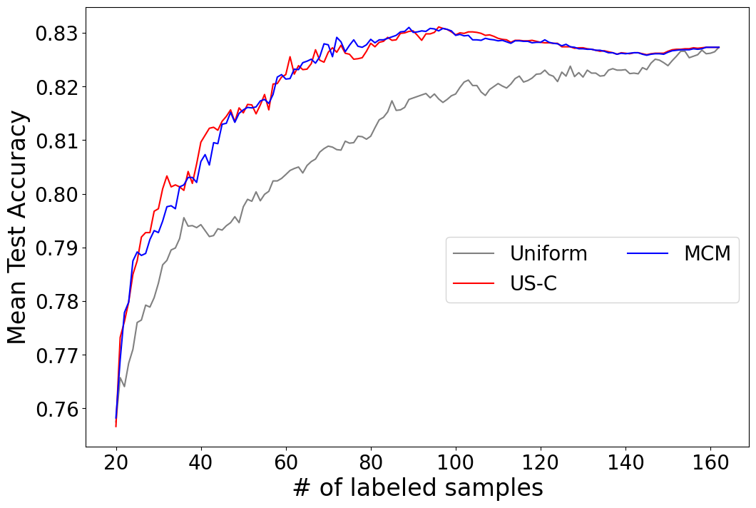
Figure 2: The learning curves (test accuracy v.s. number of queried samples) of query strategies on Heart

3 Experimental settings

This work follows most settings in [60] to reproduce and address the discrepancies observed in the existing benchmarks. To exclude the effectiveness of machine learning models, we adopt the SVM(RBF) with default hyper-parameters in scikit-learn as a task-oriented model for all experiments. Despite SVM(RBF) being a longstanding and straightforward model, it holds significant research value in recent applications [15, 9, 50].

To simulate the pool-based active learning scenarios, we split $40\%$ of a dataset to test set for evaluation and randomly sample $20$ examples from remaining as the initial labeled pool. Our benchmark compares $17$ query strategies, US-C, US-NC, QBC, VR, EER, Core-Set, Graph, Hier, HintSVM, QUIRE, DWUS, InfoDiv, MCM, BMDR, SPAL, ALBL, and LAL, described in Section 2 with default hyper-parameters in modules. We set up a budget equal to the size of the initial unlabeled pool for all experiments. The following paragraph discusses the issues discovered during the re-benchmarking process and how we addressed them.

Focus on fundamental binary classification. Zhan et al. [60] use ALiPy [46], which implemented Batch Mode Active Learning (BMDR) [52], SPAL, and LAL for binary classification. It is unclear how Zhan et al. [60] managed to provide multi-class results for these query strategies. We focus our re-benchmark on binary-class datasets and exclude multi-class datasets from the evaluation. Evaluating query strategies without supporting multi-class could impact the validity of claims when comparing and averaging results across different aspects. Therefore, we restrict our evaluation to binary-class datasets to ensure consistency and fairness.

Make the best-fit configuration for the query strategy. We encountered discrepancies between the implementation and reported in [60]. For example, we found that the Margin implemented by Google [57] is uncertainty sampling based on margin score instead of “selecting a batch of samples to optimize the marginal probability similarity between the labeled and unlabeled sets using Maximum Mean Discrepancy optimization” described in previous report [60] (See more revisions in Appendix A.4). The research community can accurately understand and evaluate findings in benchmark when consistent between the report and implementation, contributing to further research, improvement, and application.

Align the input and models of the experiments. We ensure consistency in the source datasets and the composition of the initial labeled and unlabeled pools. For instance, it is unclear whether the existing benchmark used raw data or scaled data in LIBSVM Dataset. By reviewing their released code line by line, we align our experiments based on the same input data. Besides, we notice more differences in inputs for the benchmark. For example, They apply mean removal and unit variance scaling to achieve standardized features in the pre-processing steps and specify that the initial labeled pool has a fixed size of $|D_{\text{l}}^{(0)}|=20$. We also highlighted differences between the task-oriented and query-oriented models for specific query strategies in Appendix A. We disclose the construction of the initial labeled pool, data pre-processing steps, and the choice of models, which can significantly impact the experimental results [22]. This information saves participants time examining the settings and critical considerations for designing active learning experiments.

Handle errors and exceptions of experiments. Given that different random seeds can generate problems of varying difficulty, we run the experiments $150/15$ times to mitigate issues that may arise due to lack of class in random training and testing splits, which current modules cannot support cold-start problems, or unexpected errors occurring by modules’ implementation (See Appendix D). Then, we preserve the first accomplished $100/10$ experiments to skip some failed experiments for small/large datasets to align the same experimental times with [60]. Additionally, we set a maximum running time of $1080$ hours for executing a query strategy on a dataset to ensure that the reproducing work can be completed within a feasible time. (Denote ‘TLE’ in Table 3)

The preceding paragraph outlines the necessary information to conduct experiments for the benchmark. In our implementation and report, we strive to ensure the reproducibility of all results under these specific settings and processes corresponding to Figure 1. Furthermore, we address the remaining revisions to the existing benchmark in Appendix A, covering any additional modifications or improvements needed.

4 Re-Benchmarking results

In this section, we compare our reproduced results and the disclosed report in [60] to verify whether the claims still hold (See the detailed re-benchmarking process in Appendix B). The failure of reproduction indicates potential differences between ours and the existing benchmark.

Zhan et al. [60] proposed the Beam-Search Oracle (BSO) to approximate the optimal sequence of queried samples that maximizes performance on the testing set, aiming to assess the potential improvement space for query strategies on specific datasets. To ensure a comprehensive comparison of the reproducibility of our benchmark, we implement and include BSO in this work. Our re-benchmarking results are reported in Table 1.

Table 1: Re-Benchmarking results of [60]’s Table 3. The numbers are mean AUBC ($\uparrow$, %). We denote “*” when there is a statistically significant difference between ours and [60]. We report the baseline method (Uniform), the near-optimal method (BSO), the average of mean AUBC of the $17$ query strategies , excluded Uniform and BSO (Avg), the best query strategy with its mean AUBC (BEST, BEST_QS), and the worst query strategy with its mean AUBC (WORST, WORST_QS) across datasets in Table 1. See detailed statistical hypothesis test and [60]’s table in Appendix B.1.

	Uniform	BSO	Avg	BEST	BEST_QS	WORST	WORST_QS
Appendicitis	83.95	88.37	84.25	84.57	MCM*	83.90	HintSVM*
Sonar	74.63*	88.40*	75.60	77.62	US-C*	73.57	HintSVM
Parkinsons	83.05*	88.28*	83.97	85.31	US-C*	81.78	HintSVM
Ex8b	88.53*	93.76*	88.88	89.81	US-C*	86.99	HintSVM
Heart	80.51	89.30*	80.99	81.57	US-C*	80.39	HintSVM*
Haberman	73.08	78.96*	72.95	73.19	BMDR	72.44	QUIRE
Ionosphere	91.80*	95.45*	91.59	93.00	US-C*	87.93	DWUS*
Clean1	81.83*	92.19*	81.97	84.25	US-C*	76.95	HintSVM
Breast	96.16*	97.60*	96.19	96.32	US-C*	95.82	VR*
Wdbc	95.39	98.41*	95.87	96.52	US-C*	95.04	DWUS*
Australian	84.83	90.46*	84.82	85.04	US-C*	84.44	HintSVM*
Diabetes	74.24*	82.57*	74.42	74.91	Core-Set	72.27	DWUS*
Mammographic	81.30*	85.03*	81.44	81.78	MCM	79.99	DWUS*
Ex8a	85.39*	88.28*	84.62	87.88	US-C*	79.11	DWUS*
Tic	87.18	90.77*	87.17	87.20	US-C*	86.99	QUIRE
German	73.40*	82.08*	73.65	74.17	US-C*	72.68	DWUS
Splice	80.75	91.02*	80.08	82.34	MCM*	75.18	Core-Set*
Gcloudb	89.52	90.91*	89.20	89.81	US-C*	87.48	HintSVM
Gcloudub	94.37	96.83*	93.72	95.60	US-C*	89.29	Core-Set*
Checkerboard	97.81	99.72*	96.42	98.74	Core-Set	90.45	DWUS*
Spambase	91.03*	-	91.14	92.05	US-C*	89.85	HintSVM*
Banana	89.26	-	86.90	89.30	Core-Set*	80.50	US-NC*
Phoneme	82.54	-	82.49	83.59	MCM*	80.83	HintSVM
Ringnorm	97.76*	-	97.05	97.86	US-C*	93.46	DWUS
Twonorm	97.53	-	97.54	97.64	US-C*	97.31	DWUS
Phishing	93.82*	-	93.65	94.60	US-C*	89.23	DWUS*

Table 1 demonstrates a large discrepancy from scores reported in [60] on Uniform, which is the baseline on most benchmarks. We notice an implementation error in the existing benchmark because unshuffled data does not conform to the design of the Google module. More details can be found in Appendix A.3. We want to emphasize the importance of verifying the correctness of the baseline for a benchmark through this example.

Zhan et al. [60] show that the best query strategy could achieve close AUBC as the BSO on Ionosphere, Breast, and Tic, i.e., the difference between BEST and BSO in Table 1 is less than $1\%$. However, our results show that all query strategies are less than BSO, with $1\%$ more on all datasets. This evidence indicates that there is still much room for improving active learning algorithms.

5 Beyond the re-benchmarking results

Table 1 demonstrates that the uncertainty sampling (US-C) achieves the highest average AUBC than other query strategies on most datasets, which differs from the existing benchmark [60]. In this section, we first study the different results caused by the setting of non-compatible models, then verify the superiority between query strategies to show that the US-C achieves competitive results. Furthermore, we investigate whether existing query strategies bring the benefits of using less labeled samples than Uniform to check their usefulness.

5.1 Impact of non-compatible models for uncertainty sampling

In the previous section, the results of US-C and US-NC show that the non-compatible models impact uncertainty sampling. Table 2 illustrates the relationship of settings between benchmarks. The main difference between US-C and US-NC is the query-oriented model. Specifically, US-NC adopts LR($C=0.1$) for the query-oriented and SVM(RBF) for the task-oriented model. Figure 3 illustrates that this particular setting can lead the query-oriented model to query samples that are not the most uncertain for the task-oriented model. Therefore, we conclude that the ‘non-compatible models’ lead to worse performance in the existing benchmark than ours.

Table 2: Different settings between [60] and ours

	Margin ([60] )	US ([60]) or US-NC (Ours)	US-C (Ours)
Query-oriented model	LR($C=1$)	LR($C=0.1$)	SVM(RBF)
Uncertainty measurement	margin score	entropy	margin score

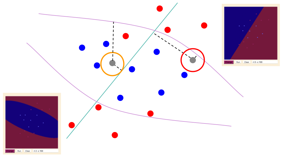
Figure 3: Given SVM(RBF) as the task-oriented model, we study the non-compatible query-oriented model with LR($C=0.1$). The red and blue points represent labeled examples. The gray points represent unlabeled examples. The cyan and megenta lines mean the decision boundaries of query models LR($C=0.1$) and SVM(RBF) trained on current labeled examples. If we adopt US, the non-compatible setting queries a sample (orange circle), which is most to LR($C=0.1$), rather than the most uncertain sample to SVM(RBF) (red circle).

To verify that non-compatible models dramatically drop the uncertainty sampling performance, we conduct experiments involving different combinations of query-oriented and task-oriented models. These combinations were based on LR, SVM(RBF), and Random Forest (RF) with default hyper-parameters in scikit-learn. The outcomes are shown in Figure 4, leading us to conclude that the performance drop from US-C to US-NC can be attributed to non-compatible query-oriented and task-oriented models. Please see more experimental results in Appendix B.2.

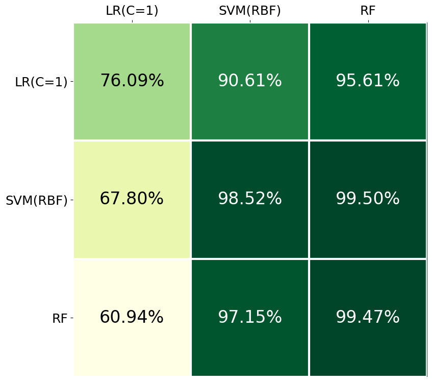
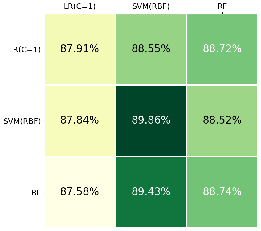
Figure 4: Mean AUBC of query-oriented model (rows) and task-oriented model (columns) on Checkerboard (left) and Gcloudb (right)

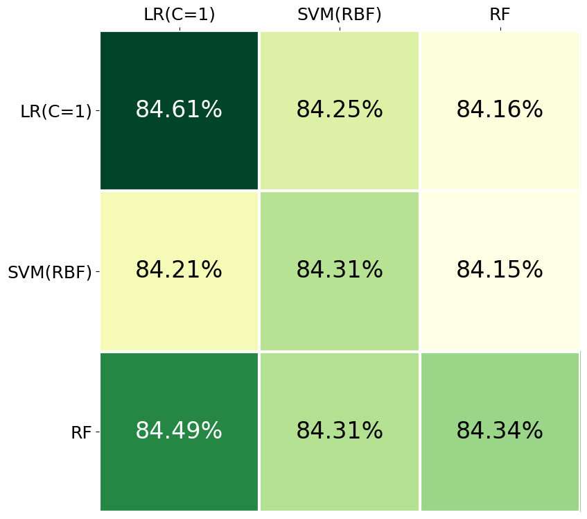
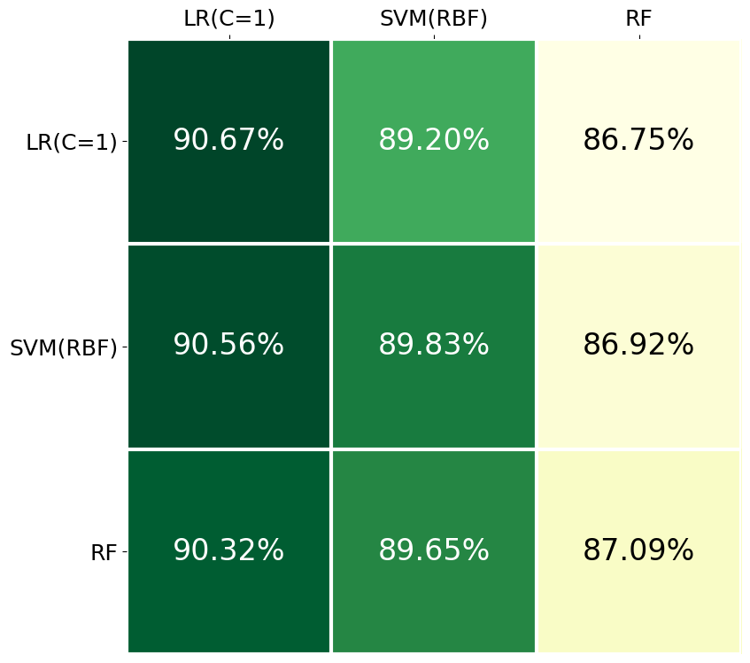
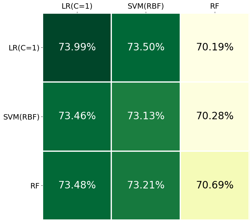
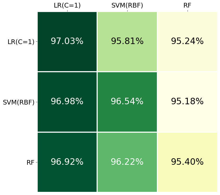
Figure 7: Mean AUBC of query-oriented model and task-oriented model on group 1. (Compatible LRs achieve best results.): Appendicitis (top-left), Ex8b (top-right), Haberman (bottom-left), and Wdbc (bottom-right).

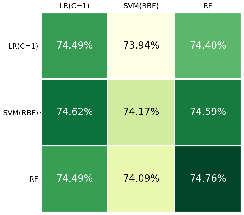
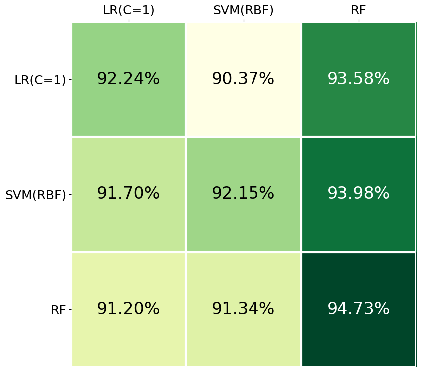
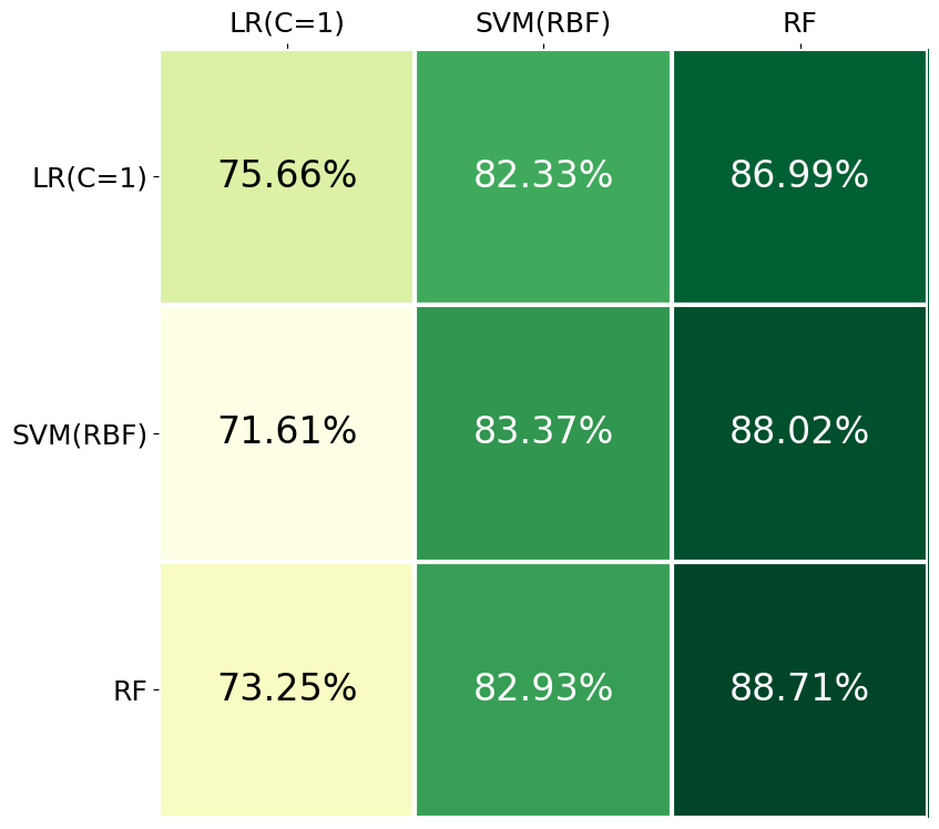
Figure 11: Mean AUBC of query-oriented model and task-oriented model on group 3. (Compatible RFs achieve best results.): German (top-left), Spambase (top-right), Phoneme (bottom-left), and Phishing (bottom-right).

Our results show that compatible models perform better than non-compatible models for uncertainty sampling on $22$ datasets. Specifically, the best AUBC score occurs at the diagonal from Figure 7 to Figure 11. Some results demonstrate that non-compatible models are slightly better than compatible models, such as Splice and Banana in Figure 12. When query-oriented and task-oriented models are heterogeneous, we conjecture that it could improve uncertainty sampling by exploring more diverse examples like the hybrid criteria approach [42, 45]. Although these observations illustrate some potential improvement and benefits from uncertainty sampling, we suggest setting compatible models for uncertainty sampling at default for a fair comparison.

5.2 Verifying superiority

Next, we verify that the US-C outperforms other query strategies on benchmark datasets. Besides comparing the mean AUBC between each query strategy in Table 1, we verify the ranking performance of query strategies across multiple datasets. Specifically, we assess the average and standard deviation of ranking by seeds of the query strategy on each dataset, then adopt the Friedman test with $5\%$ significance level to test for statistical significance. The p-values of the Friedman test are less than $5\%$ for all datasets, meaning the performance between query strategies is statistically different. Table 3 demonstrates that uncertainty sampling outperforms other query strategies on most datasets. MCM and QBC often achieve second and third ranks.

Table 3: Average Ranking of Query Startegies: We report top eight query strategies with best average ranking. The scores with ¹, ², or ³ mean the 1st, 2nd and 3rd performance on a dataset. ‘TLE’ means a query strategy exceeds the time limit.)

	US-C	MCM	QBC	EER	SPAL	VR	LAL	BMDR
Appendicitis	7.022	6.921	7.60	7.40	8.64	8.17	7.383	8.02
Sonar	3.061	4.002	5.66	8.38	9.60	9.89	5.653	7.66
Parkinsons	2.621	2.682	6.12	5.92	8.56	10.35	5.543	8.83
Ex8b	4.121	4.432	6.29	6.20	9.68	9.00	6.123	8.18
Heart	5.401	5.602	6.703	8.48	7.89	9.21	6.88	9.12
Haberman	8.12	8.00	7.52	7.152	7.70	7.223	7.131	7.25
Ionosphere	2.941	3.232	4.303	5.71	6.66	8.59	4.95	12.23
Clean1	2.411	2.602	4.083	7.06	10.95	TLE	4.38	8.82
Breast	6.141	6.202	6.343	6.94	6.72	8.96	8.88	9.09
Wdbc	2.191	2.632	4.813	5.09	9.43	11.04	6.22	12.76
Australian	6.281	6.463	7.34	8.72	6.412	8.14	8.21	8.71
Diabetes	6.122	6.483	6.71	7.71	7.07	9.24	7.49	9.10
Mammographic	5.642	5.491	6.123	6.62	8.13	9.39	7.04	8.93
Ex8a	1.541	2.102	5.403	7.75	6.93	6.90	11.59	7.10
Tic	7.102	7.031	7.42	7.74	9.14	7.51	7.46	7.27
German	4.181	4.602	5.843	6.82	7.98	9.41	6.19	9.16
Splice	2.142	2.011	4.113	6.83	8.63	6.86	7.55	9.28
Gcloudb	3.341	3.842	5.18	7.62	9.23	6.84	8.05	7.20
Gcloudub	1.431	1.902	3.133	8.65	12.33	7.38	5.28	8.82
Checkerboard	3.212	3.483	8.33	3.88	error	6.62	9.90	4.29
Spambase	1.301	2.002	2.753	TLE	TLE	TLE	7.80	TLE
Banana	6.60	8.60	4.20	TLE	TLE	3.60	3.403	TLE
Phoneme	1.802	1.501	2.903	TLE	TLE	TLE	5.90	TLE
Ringnorm	1.301	2.702	4.30	TLE	TLE	TLE	2.803	TLE
Twonorm	2.001	2.802	3.80	TLE	TLE	TLE	3.303	TLE
Phishing	1.001	2.202	3.003	TLE	TLE	TLE	4.00	TLE

Table 1 and Table 3 show that the simple and efficient uncertainty sampling overcomes others on most datasets. These outcomes also correspond to previous work that claims uncertainty sampling with logistic regression is the strong baseline [54]. We suggest that practitioners in active learning compare their query strategy with uncertainty sampling. Further, we should take uncertainty sampling as the first choice for the new task.

5.3 Verifying usefulness

In addition to comparative results between query strategies, the analysis of usefulness could uncover which query strategy could bring more benefit than Uniform and rescue practitioners from decidophobia of many methods. We study the degree of improvement over Uniform for the query strategy. Specifically, we define the difference AUBC between a query strategy $q$ and Uniform on a dataset $s$ with seed $k$ $\tau_{q,s,k}=\text{AUBC}_{q,s,k}-\text{AUBC}_{\text{Uniform},s,k}.$ We also calculate the mean $\bar{\tau}_{q,s}$ and standard deviation $\text{SD}(\tau)_{q,s}$ of $\tau_{q,s,k}$ by seeds.

We put the complete results of $\bar{\tau}_{q,s}$ and $\text{SD}(\tau)_{q,s}$ online15. Then, we apply a paired $t$-test to verify the improvement under the significance level $5\%$ on all datasets and summarize the table by counting the number of significant improvements in the aspect of a dataset and a query strategy in Figure 5. From the query strategy aspect, Figure 5 demonstrates that VR, Graph, Hier, DWUS, HintSVM, BMDR, and QUIRE are not competitive with Uniform on more than $21$ ($80\%$) datasets. Moreover, SPAL, Core-Set, and EER are not significantly better than Uniform on less than $16$ ($60\%$) datasets. The results indicate that the complicated design of query strategies, such as VR, QUIRE, BMDR, and SPAL, can not improve performance in the current settings. In contrast, hyper-parameters-free and efficient uncertainty sampling performs effectively on most datasets.

Even though uncertainty sampling outperforms other query strategies on most datasets, from the dataset aspect, Figure 5 reveals the difficulty of this query strategy on Haberman, Tic, Banana, and Ringnorm, in which less than three ($20\%$) query strategies are significantly better than Uniform. The complicated problem in Banana is also revealed in [13], which is still an unsolved challenge for practitioners uneasy about using active learning for real-world problems. The results indicate that the practitioners still need a more robust baseline than uncertainty sampling under scenarios where active learning might fail.

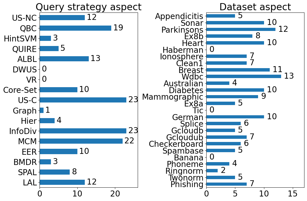
Figure 5: Number of significant improvements of Query Strategy from Uniform

6 Conclusion

The work offers the community a transparent and reproducible benchmark for active learning. The benchmark is based on our meticulous re-examination of existing benchmarks to resolve the discrepancies. Through our re-benchmarking efforts, several valuable insights have been obtained. Firstly, our benchmark challenges the previously claimed superiority of the Learning Active Learning strategy, restoring the competitiveness of the uncertainty sampling strategy in the realm of active learning. Secondly, we have uncovered the significant impact of compatibility between query-oriented and task-oriented models on the effectiveness of uncertainty sampling. Thirdly, by carefully comparing active learning strategies with the passive baseline of uniform sampling, we have revealed that more than half ($10$) of the examined active learning strategies do not exhibit significant advantages over the passive baseline. These findings not only enrich the community’s understanding of existing active learning solutions but also lay the foundation for future research with our open-sourced and extensible benchmark. Our experience underscores the essential nature of re-benchmarking in upgrading benchmarks with more reliable implementations and enabling deeper understanding.

In summary, in this work, we provide a transparent, reliable, and reproducible active learning benchmark platform, which enhances our understanding of active learning algorithms. We envision our framework can be further extended to include different domains, such as vision and languages, and other models, such as deep neural networks, as detailed in Appendix E for future research.

Appendix A Revision of [60]

In this section, we reveal and revise descriptions in [60] to provide clear information to readers and the active learning community. Furthermore, Zhan et al. [60] published their source code on GitHub in March, thus we study the difference of Uniform on Table 1.

A.1 Experimental Settings in [60]

Inputs and base models. As illustrated in Figure 1, Zhan et al. [60] employed a random split of $60\%$ of the dataset for the training set while the remaining $40\%$ for the testing set. No pre-processing was applied to the dataset, and fixed random seeds were used to ensure consistency in the training and testing sets across repeated experiments. They used an SVM with an RBF kernel (SVM(RBF)) as the task-oriented model for evaluating the query strategies.

Query strategies. To compare the performance of $17$ query strategies, they implemented random sampling and all query strategies using different libraries. The libact library provided implementations for Uncertainty Sampling (US), Query by Committee (QBC), Hinted Support Vector Machine (HintSVM), Querying Informative and Representative Examples (QUIRE), Active Learning by Learning (ALBL), Density Weighted Uncertainty Sampling (DWUS), and Variation Reduction (VR). The Google library included Random Sampling (Uniform), k-Center-Greedy (KCenter), Margin-based Uncertainty Sampling (Margin), Graph Density (Graph), Hierarchical Sampling (Hier), Informative Cluster Diverse (InfoDiv), and Representative Sampling (MCM). The ALiPy library contributed Estimation of Error Reduction (EER), BMDR, SPAL, and LAL. Besides, they proposed the Beam-Search Oracle (BSO) as a reference to approximate the optimal sequence of queried samples that maximizes performance on the testing set, aiming to assess the potential improvement space for query strategies on specific datasets.

Through reviewing the released source code in [60], we identified differences between the task-oriented and query-oriented models for specific query strategies. Table 4 highlights the discrepancies between the two models for each query strategy. In particular, Margin and US (US-C and US-NC in our work) are variant settings for uncertainty sampling. We further discuss such differences in Section 5.1. For the unrevealed information of remaining query strategies, we adopt SVM(RBF) for a query strategy and evaluation by default.

Table 4: Non-Compatible query-oriented model $\mathcal{H}$ and task-orienged model $\mathcal{G}$, SVM(RBF, gamma = ‘auto’), for a query strategy $\mathcal{Q}$

$\mathcal{Q}$	$\mathcal{H}$
US([60]) , US-NC (Ours)	LR($C=0.1$)
QBC	LR($C=1$), SVM(Linear, probability = True), SVM(RBF, probability = True), Linear Discriminant Analysis
ALBL	Combination of QSs with same $\mathcal{H}$: US-C, US-NC, HintSVM
VR	LR($C=1$)
EER	SVM(RBF, probability = True)

Experimental design. The active learning algorithm was stopped when the total budget was equal to the size of the unlabeled pool, that is, $T=|D_{\text{u}}^{(0)}|$. They collected the testing accuracy at each round to constructing a learning curve, and the AUBC was calculated to summarize the performance of a query strategy on a dataset. To ensure reliable results, they conducted $K_{\text{S}}=100$ repeated experiments for small datasets ($n<2000$) and $K_{\text{L}}=10$ repeated experiments for large datasets ($n\geq 2000$), where $n$ represents the size of the dataset. Finally, they compute the average AUBCs across repeated experiments for each query strategy on each dataset.

Analysis methods. Zhan et al. [60] benchmarked the pool-based active learning for classifications on $35$ datasets, including $26$ binary-class and $9$ multi-class datasets collected from LIBSVM and UCI [7, 16]. They provided the data properties, such as the number of samples $n$, dimension $d$, and imbalance ratio IR, where the imbalance ratio is the proportion of the number of negative labels to the number of positive labels

$$\text{IR}=\frac{|\{(x_{i},y_{i}):y_{i}=+1\}|}{|\{(x_{j},y_{j}):y_{j}=-1\}|}.$$

They employed these metrics to analyze the results from different aspects to explain the results of the query strategy’s performance on a dataset. Their work is valuable for its large-scale experiments on many datasets and analysis methods, identifying applicability factors, and understanding the room for growth of various query strategies.

We agree with their core idea of the analysis methods and believe their benchmark benefits the research community. However, we observe that the conclusion of their work differs from several previous works. For example, Zhan et al. [60] claimed the LAL performs better on binary datasets than uncertainty sampling. The claim is inconsistent with the fact that uncertainty sampling performs well on most binary datasets [54, 13]. The evidence urges us to re-implement the active learning benchmark.

A.2 Benchmarking datasets

Section 3 records that we receive the benchmarking datasets used for the benchmark from [60], which is the same as their published source code8. However, we discover that the attributes of datasets are different. We report the change from [60] to the new version in Table 5 via ‘[60]$\rightarrow$new version’.

Table 5: Revision of Table 2 in [60]

	Property	$r$	$d$	$n$
Appendicitis	Real-life	4	7	106
Sonar	Real-life	1	60	108$\rightarrow$208
Ex8b	Synthetic	1	2	206$\rightarrow$210
Heart	Real-life	1	13	270
Haberman	Real-life	2	3	306
Ionosphere	Real-life	1	34	351
Clean1	Real-life	1	168$\rightarrow$166	475$\rightarrow$476
Breast	Real-life	1	10	478
Wdbc	Real-life	1	30	569
Australian	Real-life	1	14	690
Diabetes	Real-life	1	8	768
Mammographic	Real-life	1	5	830
Ex8a	Synthetic	1	2	863$\rightarrow$766
Tic	Real-life	6	9	958
German	Real-life	2	20$\rightarrow$24	1000
Splice	Real-life	1	61$\rightarrow$60	1000
Gcloudb	Synthetic	1	2	1000
Gcloudub	Synthetic	2$\rightarrow$2.03	2	1000
Checkerboard	Synthetic	1$\rightarrow$1.82	2	1600
Spambase	Real-life	1$\rightarrow$1.54	57	4601
Banana	Synthetic	1	2	5300
Phoneme	Real-life	2	5	5404
Ringnorm	Real-life	1	21$\rightarrow$20	7400
Twonorm	Real-life	1	50$\rightarrow$20	7400
Phishing	Real-life	1	30	2456$\rightarrow$11055

A.3 Failure of the Reproducing Uniform

Table 1 (Table 9) shows the significant difference between ours and [60]. Although [60]’s code could reproduce their reported score, we noticed an implementation error. In Google, Uniform assumes that the data has already been shuffled.. However, the implementation in Zhan et al. [60] does not shuffle the unlabeled pool at first.

[Code=Python]
dict_data,labeled_data,test_data,unlabeled_data = \
    split_data(dataset_filepath, test_size, n_labeled)

print(unlabeled_data)
# results of indices of unlabeled pool
#[3, 4, 5, 10, 11, 13, 15, 16, 20, 23, 24, 26, 27, 29, 30, 31, 33, 36, 37, 41,\
# 43, 44, 45, 49, 50, 51, 53, 54, 55, 57, 63, 64, 65, 70, 73, 75, 77, 78, 79, \
# 83, 84, 86, 87, 88, 89, 91, 92, 95, 97, 102, 105, 110, 112, 114, 115, 121, \
# 122, 127, 128, 131, 132, 136, 137, 139, 140, 144, 148, 150, 151, 155, 157, \
# 159, 160, 161, 162, 164, 165, 167, 168, 172, 175, 176, 177, 178, 181, 182, \
# 183, 184, 185, 186, 187, 188, 190, 191, 193, 194, 197, 198, 199, 202, 203, \
# 204, 205, 207, 208]

We also modify their Uniform implementation through shuffle the unlabeled_data. Then we can obtain similar results to ours based on their source code, see Table 6.

[Code=Python]
dict_data,labeled_data,test_data,unlabeled_data = \
    split_data(dataset_filepath, test_size, n_labeled)
random.shuffle(unlabeled_data)

Table 6: Comparing different train/test/labeled splits on Sonar: first column is reprot and reproducing results in [60], second column in our implementation, and the third column is reproducing results after we revise [60]’s code.

Uniform	Report and code in [60]	Our code	Modified code in [60]
Google	0.6274*	0.7513	0.7577
libact	-	0.7520	0.7543
ALiPy	-	0.7556	0.7579

The unshuffled implementation in Google significantly impacts the binary classification datasets, such as Sonar, Clean1, Spambase, also affects Ex8a and German, which enlarge the difference AUBCs between Uniform and other query strategies. Due to this experience, we suggest practitioners ensure the correctness of the baseline method by comparing different implementations before conducting the benchmarking experiments.

A.4 Query Strategy and Implementation

We revise some description of the query strategies in [60]:

1. ‘Graph Density (Graph) is a typical parallel-form combined strategy that balances the uncertainty and representative based measure simultaneously via a time-varying parameter [17].’

2. ‘Marginal Probability based Batch Mode AL (Margin) Chattopadhyay et al. [8] selects a batch that makes the marginal probability of the new labeled set similar to the one of the unlabeled set via optimization by Maximum Mean Discrepancy (MMD).’

3. ‘Kremer et al. [27] proposed an SVM-based AL strategy by minimizing the distances between data points and classification hyperplane (HintSVM).’

Issue (1): Although Ebert et al. [17] proposes the reinforcement learning method to select uncertainty and diversity sample(s) during the procedure, Google [57] does not implement the whole procedure but only the diversity sampling method. Thus, we should categorize it as diversity-based method.
Issue (2): Google [57] does not use MMD to measure the distance. The implementation is uncertainty sampling with margin score is mentioned in the survey paper [42]. Therefore, we should categorize it to uncertainty-based method.
Issue (3): libact [56] implemented HintSVM based on the work [29] rather than [27].

A.5 Relationship between query strategies

We provide additional evidence to explain the relationship between query strategies, which supports our experimental results.

1. US-C and InfoDiv should be the same when the query batch size is one.

2. Use different uncertainty measurements should be the same in the binary classification. This indicates different uncertainty measurements do not cause the difference between US-C and US-NC.

3. SPAL changes the condition of variables, which are used for discriminative and representative objective functions in BMDR.

Issue (1): InfoDiv clusters unlabeled samples into several clusters, then select uncertain samples and keep the same cluster distribution simultaneously. Therefore, it is the same when we set the $B=1$ to query the most uncertain sample. Zhan et al. [60] provides the different numbers of US-C and InfoDiv in Table 4. They might not use the same batch size of these query strategies.
Issue (2): The least confidence, margin, and entropy are monotonic functions with peak equal to $\mathbb{P}(y=+1\mid x)=0.5$ in binary classification, such that all of these uncertainty measurements would query the same point [42].
Issue (3) The optimization problem in BMDR is:

$$\begin{split}\min_{\alpha^{\top}1_{|D_{u}|}=b,w}&\sum_{i=1}^{|D_{l}|}(y_{i}-w^{\top}\phi(x_{i}))^{2}+\lambda\|w\|^{2}\\ &+\sum_{i=1}^{|D_{u}|}\alpha_{i}\left[\|w^{\top}\phi(x_{j})\|^{2}_{2}+2|w^{\top}\phi(x_{j})|\right]\\ &+\beta(\alpha^{\top}K_{1}\alpha+k\alpha),\end{split}$$ (1)

where $\phi(x)$ is the feature mapping, $\lambda$ is the hyper-parameter for the regularization term, $\beta$ if the hyper-parameter for the diversity term, $1_{|D_{u}|}$ means ones vector with length of the unlabelled pool $|D_{u}|$. $K_{1}$ is defined as $K_{1}=\frac{1}{2}K_{UU}$, where $K_{UU}$ means the kernel matrix with sub-index $U$ of unlabelled pool $D_{u}$. SPAL only change $\alpha^{\top}1_{|D_{u}|}=b$ to $\alpha^{\top}e_{|D_{u}|}=b$.

A.6 Comparison between [60] and [54]

Yang and Loog [54] propose the first benchmark for pool-based active learning for the conventional Logistic Regression model. The work compares $10$ query strategies that could be categorized into model uncertainty and hybrid criteria. In datasets, they adopt 44 binary datasets and follow data pre-processing in [7]. To compare performance across different query strategies, they also use an Area Under the Learning Curve with accuracy to show the average performance of a query strategy, named AUBC in [60]. Furthermore, they compare the performance of each query strategy by average rank and improvement (win/tie/loss) from random sampling, which has the same purpose as our work (See Section 5.2 and Section 5.3).

Table 7: Comparison between [54, 60] and our benchmark. QS is abbreviation of query strategy.

	[54]	Zhan et al. [60]	Ours
Binary datasets	44	35	26
Multi-class datasets	0	9	0
Task-oriented model	LR	SVM(RBF)	SVM(RBF)
Model uncertainty (QS)	✓	✓	✓
Data diversity (QS)	✗	✓	✓
Hybrid criteria (QS)	✓	✓	✓
Redesigned learning framework (QS)	✗	✓	✓
AUBC (evaluation)	✓	✓	✓
Average ranking (evaluation)	✓	✗	✓
Comparison with Uniform (evaluation)	✓	✗	✓

Appendix B Detailed re-benchmarking results

After we accomplish experiments under the settings in Section 3, we obtain the benchmarking results with the form (query strategy, dataset, seed, $|D_{l}|$, accuracy) for each round. A (random) seed corresponds to the different training sets, test sets, and initial label pool splits for a dataset. We collect the accuracy at each round ($|D_{\text{l}}|$, accuracy). to plot a learning curve for query strategy on a dataset with a seed and summarize it as the AUBC.

To construct Table 1, we average the AUBC by seed. We denote the table of (query strategy, dataset) as the summary table, including mean and standard deviation (SD) AUBC of a query strategy on each dataset. The summary table is released online to make the performance of a query strategy on a dataset transparent to readers. Based on the summary table, we reproduce results of [60] in Table 1.

B.1 Statistical comparison of benchmarking results

Table 1 demonstrates we fail to reproduce Uniform, the baseline method, on $13$ datasets. We show our Table 1 side-by-side with [60]’s Table 3 in detail (See Table 8). To determine if there is a statistical difference between the two benchmarking results, we construct the confidence interval with $t$-distribution of mean AUBCs. If a result in [60] falls outside the interval, their mean significantly differs from ours.

Table 8: We report AUBCs ($\%$) in Table 1 and in [60]’s Table 3 side-by-side. A score denoted with format:[60] $\rightarrow$ ours.

	Uniform	BSO	Avg	BEST	BEST_QS	WORST	WORST_QS
Appendicitis	84 $\rightarrow$ 83.95	88 $\rightarrow$ 88.37	84 $\rightarrow$ 84.25	86 $\rightarrow$ 84.57	EER $\rightarrow$ MCM*	83 $\rightarrow$ 83.90	DWUS $\rightarrow$ HintSVM*
Sonar	62 $\rightarrow$ 74.63*	83 $\rightarrow$ 88.40*	76 $\rightarrow$ 75.60	78 $\rightarrow$ 77.62	LAL $\rightarrow$ US-C*	73 $\rightarrow$ 73.57	HintSVM $\rightarrow$ HintSVM
Parkinsons	84 $\rightarrow$ 83.05*	87 $\rightarrow$ 88.28*	85 $\rightarrow$ 83.97	86 $\rightarrow$ 85.31	QBC $\rightarrow$ US-C*	83 $\rightarrow$ 81.78	HintSVM $\rightarrow$ HintSVM
Ex8b	87 $\rightarrow$ 88.53*	92 $\rightarrow$ 93.76*	89 $\rightarrow$ 88.88	91 $\rightarrow$ 89.81	SPAL $\rightarrow$ US-C*	86 $\rightarrow$ 86.99	HintSVM $\rightarrow$ HintSVM
Heart	81 $\rightarrow$ 80.51	85 $\rightarrow$ 89.30*	79 $\rightarrow$ 80.99	83 $\rightarrow$ 81.57	InfoDiv $\rightarrow$ US-C*	72 $\rightarrow$ 80.39	DWUS $\rightarrow$ HintSVM*
Haberman	73 $\rightarrow$ 73.08	75 $\rightarrow$ 78.96*	73 $\rightarrow$ 72.95	74 $\rightarrow$ 73.19	BMDR $\rightarrow$ BMDR	72 $\rightarrow$ 72.44	QUIRE $\rightarrow$ QUIRE
Ionosphere	90 $\rightarrow$ 91.80*	93 $\rightarrow$ 95.45*	91 $\rightarrow$ 91.59	93 $\rightarrow$ 93.00	LAL $\rightarrow$ US-C*	88 $\rightarrow$ 87.93	HintSVM $\rightarrow$ DWUS*
Clean1	65 $\rightarrow$ 81.83*	87 $\rightarrow$ 92.19*	81 $\rightarrow$ 81.97	84 $\rightarrow$ 84.25	LAL $\rightarrow$ US-C*	75 $\rightarrow$ 76.95	HintSVM $\rightarrow$ HintSVM
Breast	95 $\rightarrow$ 96.16*	96 $\rightarrow$ 97.60*	96 $\rightarrow$ 96.19	96 $\rightarrow$ 96.32	SPAL $\rightarrow$ US-C*	95 $\rightarrow$ 95.82	DWUS $\rightarrow$ VR*
Wdbc	95 $\rightarrow$ 95.39	97 $\rightarrow$ 98.41*	96 $\rightarrow$ 95.87	97 $\rightarrow$ 96.52	LAL $\rightarrow$ US-C*	94 $\rightarrow$ 95.04	EER $\rightarrow$ DWUS*
Australian	85 $\rightarrow$ 84.83	88 $\rightarrow$ 90.46*	85 $\rightarrow$ 84.82	85 $\rightarrow$ 85.04	Core-Set $\rightarrow$ US-C*	82 $\rightarrow$ 84.44	DWUS $\rightarrow$ HintSVM*
Diabetes	74 $\rightarrow$ 74.24*	78 $\rightarrow$ 82.57*	74 $\rightarrow$ 74.42	75 $\rightarrow$ 74.91	Core-Set $\rightarrow$ Core-Set	69 $\rightarrow$ 72.27	EER $\rightarrow$ DWUS*
Mammographic	82 $\rightarrow$ 81.30*	84 $\rightarrow$ 85.03*	82 $\rightarrow$ 81.44	83 $\rightarrow$ 81.78	MCM $\rightarrow$ MCM	80 $\rightarrow$ 79.99	EER $\rightarrow$ DWUS*
Ex8a	84 $\rightarrow$ 85.39*	87 $\rightarrow$ 88.28*	84 $\rightarrow$ 84.62	86 $\rightarrow$ 87.88	Hier $\rightarrow$ US-C*	80 $\rightarrow$ 79.11	QUIRE $\rightarrow$ DWUS*
Tic	87 $\rightarrow$ 87.18	87 $\rightarrow$ 90.77*	87 $\rightarrow$ 87.17	87 $\rightarrow$ 87.20	EER $\rightarrow$ US-C*	87 $\rightarrow$ 86.99	QUIRE $\rightarrow$ QUIRE
German	73 $\rightarrow$ 73.40*	78 $\rightarrow$ 82.08*	74 $\rightarrow$ 73.65	74 $\rightarrow$ 74.17	QBC $\rightarrow$ US-C*	72 $\rightarrow$ 72.68	DWUS $\rightarrow$ DWUS
Splice	81 $\rightarrow$ 80.75	87 $\rightarrow$ 91.02*	79 $\rightarrow$ 80.08	82 $\rightarrow$ 82.34	QBC $\rightarrow$ MCM*	68 $\rightarrow$ 75.18	EER $\rightarrow$ ore-Set*
Gcloudb	89 $\rightarrow$ 89.52	90 $\rightarrow$ 90.91*	89 $\rightarrow$ 89.20	90 $\rightarrow$ 89.81	Graph $\rightarrow$ US-C*	87 $\rightarrow$ 87.48	HintSVM $\rightarrow$ HintSVM
Gcloudub	94 $\rightarrow$ 94.37	96 $\rightarrow$ 96.83*	93 $\rightarrow$ 93.72	95 $\rightarrow$ 95.60	QBC $\rightarrow$ US-C*	86 $\rightarrow$ 89.29	EER $\rightarrow$ ore-Set*
Checkerboard	98 $\rightarrow$ 97.81	99 $\rightarrow$ 99.72*	94 $\rightarrow$ 96.42	99 $\rightarrow$ 98.74	Core-Set $\rightarrow$ Core-Set	90 $\rightarrow$ 90.45	VR $\rightarrow$ DWUS*
Spambase	69 $\rightarrow$ 91.03*	- $\rightarrow$ -	88 $\rightarrow$ 91.14	92 $\rightarrow$ 92.05	QBC $\rightarrow$ US-C*	69 $\rightarrow$ 89.85	DWUS $\rightarrow$ HintSVM*
Banana	90 $\rightarrow$ 89.26	- $\rightarrow$ -	85 $\rightarrow$ 86.90	89 $\rightarrow$ 89.30	Hier $\rightarrow$ Core-Set*	78 $\rightarrow$ 80.50	QUIRE $\rightarrow$ US-NC*
Phoneme	82 $\rightarrow$ 82.54	- $\rightarrow$ -	82 $\rightarrow$ 82.49	83 $\rightarrow$ 83.59	QBC $\rightarrow$ MCM*	80 $\rightarrow$ 80.83	HintSVM $\rightarrow$ HintSVM
Ringnorm	98 $\rightarrow$ 97.76*	- $\rightarrow$ -	95 $\rightarrow$ 97.05	98 $\rightarrow$ 97.86	LAL $\rightarrow$ US-C*	80 $\rightarrow$ 93.46	DWUS $\rightarrow$ DWUS
Twonorm	98 $\rightarrow$ 97.53	- $\rightarrow$ -	98 $\rightarrow$ 97.54	98 $\rightarrow$ 97.64	Core-Set $\rightarrow$ US-C*	97 $\rightarrow$ 97.31	DWUS $\rightarrow$ DWUS
Phishing	93 $\rightarrow$ 93.82*	- $\rightarrow$ -	94 $\rightarrow$ 93.65	95 $\rightarrow$ 94.60	LAL $\rightarrow$ US-C*	92 $\rightarrow$ 89.23	Graph $\rightarrow$ DWUS*

Table 9 demonstrates our mean and standard deviation (SD) AUBC of Uniform and mean AUBC of Uniform reported in [60]. There are $11$ ($13$), nearly half of the datasets, significantly different from the existing benchmark with significance level $\alpha=1\%$ ($\alpha=5\%$). Furthermore, we perform better on most datasets except for Parkinsons and Mammographic. There are $1\%$ of mean AUBC greater than previous work on $8$ datasets, especially for Sonar, Clean1, Spambase.

Table 9: Reporducing Failure of Uniform

	Mean (%)	SD (%)	[60] (%)	$\alpha=5\%$	$\alpha=1\%$
Appendicitis	83.95	3.63	83.6	In	In
Sonar	74.63	3.79	61.7	Out	Out
Parkinsons	83.05	3.68	84.0	Out	In
Ex8b	88.53	2.80	86.6	Out	Out
Heart	80.51	2.79	80.8	In	In
Haberman	73.08	2.70	72.7	In	In
Ionosphere	91.80	1.78	90.1	Out	Out
Clean1	81.83	1.94	64.9	Out	Out
Breast	96.16	0.90	95.4	Out	Out
Wdbc	95.39	1.30	95.2	In	In
Australian	84.83	1.58	84.6	In	In
Diabetes	74.24	1.52	73.6	Out	Out
Mammographic	81.30	1.98	81.9	Out	Out
Ex8a	85.39	2.17	83.8	Out	Out
Tic	87.18	1.53	87.0	In	In
German	73.40	1.73	72.6	Out	Out
Splice	80.75	1.61	80.6	In	In
Gcloudb	89.52	1.17	89.3	In	In
Gcloudub	94.37	0.96	94.2	In	In
Checkerboard	97.81	0.59	97.8	In	In
Spambase	91.03	0.57	68.5	Out	Out
Banana	89.26	0.38	89.5	In	In
Phoneme	82.54	1.01	82.2	In	In
Ringnorm	97.76	0.21	97.6	Out	In
Twonorm	97.53	0.19	97.6	In	In
Phishing	93.82	0.48	92.6	Out	Out

Following the same procedure of statistical testing, Table 10 demonstrates BSO of ours and [60]. This phenomenon is more evident in BSO than in Uniform. We still get significantly different and better performances on most datasets except for Appendicitis.

Table 10: Reporducing Failure of BSO

	Mean (%)	SD (%)	[60] (%)	$\alpha=5\%$	$\alpha=1\%$
Appendicitis	88.37	2.95	88.1	In	In
Sonar	88.40	2.84	83.0	Out	Out
Parkinsons	88.28	3.19	86.5	Out	Out
Ex8b	93.76	1.82	92.4	Out	Out
Heart	89.30	2.47	84.8	Out	Out
Haberman	78.96	3.05	75.1	Out	Out
Ionosphere	95.45	1.42	93.3	Out	Out
Clean1	92.19	1.69	87.1	Out	Out
Breast	97.60	0.67	96.1	Out	Out
Wdbc	98.41	0.65	97.3	Out	Out
Australian	90.46	1.48	87.8	Out	Out
Diabetes	82.57	1.70	78.4	Out	Out
Mammographic	85.03	1.97	84.4	Out	Out
Ex8a	88.28	2.03	87.3	Out	Out
Tic	90.77	2.27	87.3	Out	Out
German	82.08	2.01	78.3	Out	Out
Splice	91.02	1.18	87.1	Out	Out
Gcloudb	90.91	1.09	90.1	Out	Out
Gcloudub	96.83	0.78	96.3	Out	Out
Checkerboard	99.72	0.36	99.2	Out	Out

B.2 More on analysis of non-compatible models for uncertainty sampling

Figure 4 demonstrates results involving different combinations of query-oriented and task-oriented models on Checkerboard and Gcloudb datasets. We reveal more datasets from Figure 7 to Figure 11. These results still hold for the compatible models for uncertainty sampling outperform non-compatible ones on most datasets, i.e., the diagonal entries of the heatmap are larger than non-diagonal entries. Figure 12 demonstrates non-compatible models achieve slightly better performance than compatible models. When query-oriented and task-oriented models are heterogeneous, we conjecture that it could improve uncertainty sampling by exploring more diverse examples like the hybrid criteria approach [42, 45].

B.3 More on analysis of usefulness

Figure 5 summarized the degree of improvement over Uniform for a query strategy. We report the detailed mean difference between a query strategy and Uniform on GitHub: https://github.com/ariapoy/active-learning-benchmark/tree/main/results#usefulness-of-query-strategies. We study whether a query strategy is significantly more effective than Uniform based on a pair $t$-test.

B.4 Verifying Applicability

Section 5.3 verifies that US-C, MCM, and QBC can effectively improve the testing accuracy over Uniform on most datasets. We want to analyze when these query strategies could benefit more than Uniform. Zhan et al. [60] inspired us could verify applicability by several aspects:

• Low/high dimension view (LD for $d<50$, HD for $d\geq 50$),

• Data scale view (SS for $n<1000$, LS for $n\geq 1000$),

• Data balance/imbalance view (BAL for $\gamma<1.5$, IMB for $\gamma\geq 1.5$).

They compare these aspects with a score

$$\delta_{q,s}=\max{\{\overline{\text{AUBC}_{\text{BSO},s}},\overline{\text{AUBC}_{\text{US},s}},\dots,\overline{\text{AUBC}_{\text{LAL},s}\}}}-\overline{\text{AUBC}_{q,s}},$$

Specifically, they grouped $\delta_{q,s}$ by different aspects to generate the metric for the report.

$$\bar{\delta}_{q,v}=\frac{\sum_{s\in v}\delta_{q,s}}{|\{s\in v\}|},$$

where $v$ is one of a dataset’s dimension, scale, or class-balance views. We re-benchmark results and denote the rank of the query strategy with a superscript in Table 11. Table 11 shows that the US-C (InfoDiv) and MCM occupy the first and second ranks on different aspects, and the QBC keeps the third rank. The results are unlike to [60] except for the QBC performance well on both of us. We explain the reason for the same performance of US-C and InfoDiv in Appendix A.5.

Table 11: Verifying Applicability with $\delta_{i}$

	B	LD	HD	SS	LS	BAL	IMB
US-NC	4.77	4.16	8.12	5.36	3.96	5.09	4.39
QBC	3.833	3.153	7.573	5.023	2.203	4.053	3.573
HintSVM	5.91	4.92	11.37	6.77	4.73	6.25	5.51
QUIRE	5.96	5.08	11.54	6.13	5.60	6.94	4.98
ALBL	4.20	3.49	8.06	5.37	2.59	4.45	3.90
DWUS	6.20	5.46	10.24	6.71	5.50	6.83	5.46
VR	5.04	4.26	12.02	5.43	4.13	5.36	4.72
Core-Set	4.92	3.78	11.20	5.79	3.72	5.35	4.42
US-C	3.501	2.891	6.861	4.621	1.971	3.721	3.241
Graph	4.62	3.72	9.58	5.77	3.05	4.98	4.20
Hier	4.22	3.41	8.69	5.53	2.43	4.49	3.90
InfoDiv	3.501	2.891	6.861	4.621	1.971	3.721	3.241
MCM	3.562	2.942	6.982	4.682	2.032	3.802	3.272
EER	5.21	4.18	11.09	5.33	4.86	6.13	4.30
BMDR	5.61	4.57	11.50	5.77	5.11	6.33	4.89
SPAL	5.90	4.69	12.32	5.67	6.77	6.56	5.17
LAL	4.14	3.41	8.14	5.27	2.59	4.37	3.86

Using score $\bar{\delta}_{q,v}$ to ascertain the applicability of several query strategies is straightforward. However, it could bring an issue: BSO outperforms query strategies significantly on most datasets in our benchmarking results. We cannot exclude those remaining large-scale datasets without BSO, i.e., $n>1000$, having the same pattern, such that their results could impact different aspects. Therefore, we replace $\bar{\delta}_{q,v}$ with the improvement of query strategy $q$ over Uniform, i.e., $\tau_{q,s,k}$ in Section 5.3, because Uniform is the baseline and most efficient across all experiments, which is essential to complete.

The other issue is heuristically grouping the views into a binary category and averaging the performance with the same views $\bar{\delta}_{q,v}$ without reporting SDs. These analysis methods may be biased when the properties of datasets are not balanced. To address this issue, we plot a matrix of scatter plots that directly demonstrates the improvement of US-C for each property on all datasets with different colors. Figure 6 shows a low correlation ($|r|<0.4$) and no apparent patterns between properties and the improvement of US-C. Our analysis results do not support the claims of ‘Method aspects’ in existing benchmark [60]. In conclusion, we want to emphasize that revealing the analysis methods is as important as the experimental settings because the analysis method employed will influence the conclusion.

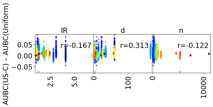
Figure 6: A matrix of scatter plots of the improvement of US-C

Appendix C Computational resource

We test the time of an experiment for query strategy running on a dataset. Our resource is: DELL PowerEdge R730 with CPU Intel Xeon E5-2640 v3 @2.6GHz * 2 and memory 192 GB. The results are reported on GitHub: https://github.com/ariapoy/active-learning-benchmark/tree/main/results#computational-time. Note that this work does not optimize libact, Google, and ALiPy performance. If practitioners discover inefficient implementation, please contact us by mail or leave issues on GitHub.

Appendix D Errors of Undone Experiments

D.1 ALiPy BMDR and SPAL

The below error occurs at BMDR or SPAL for several datasets. To realize why this error occurs, let’s review the idea of BMDR: Wang and Ye [52] proposed combining the discriminative and representative parts for querying the new sample. They solve the quadratic programming problem for the query score $\alpha$ through CVXPy [14] in Step 2. Section 3.5 [52]:

$$\min_{\alpha^{\top}\mathbf{1}_{u}}\alpha^{\top}\frac{1}{2}K_{UU}\alpha+\frac{u-b}{n}\mathbf{1}_{l}^{\top}K_{LU}\alpha-\frac{l+b}{n}\mathbf{1}_{u}^{\top}K_{UU}\alpha,$$

where $K_{\bullet\bullet}$ means the kernel matrix with sub-index of label pool $L$, unlabelled pool $U$. We trace the error occurs at CVXPy solve the quadratic form built by $K_{UU}$ during optimization procedure in ALiPy:

[Code=Python]
# results of the error occurring at CVXPy
#*** cvxpy.error.DGPError: Problem does not follow DGP rules.\
#The objective is not DGP. Its following subexpressions are not:
#var5498 <-- needs to be declared positive
#[[5.00000000e+02 9.78417179e-36 4.48512639e-06 ... 9.65890231e-07
#  1.31323498e-06 2.17454735e-06]
# [9.78417179e-36 5.00000000e+02 6.98910757e-36 ... 5.51562055e-46
#  3.34719606e-43 7.55167800e-44]
# [4.48512639e-06 6.98910757e-36 5.00000000e+02 ... 1.47944784e-06
#  1.00220776e-06 1.83491987e-05]
# ...
# [9.65890231e-07 5.51562055e-46 1.47944784e-06 ... 5.00000000e+02
#  2.61170854e-07 3.13826456e-04]
# [1.31323498e-06 3.34719606e-43 1.00220776e-06 ... 2.61170854e-07
#  5.00000000e+02 4.30837086e-08]
# [2.17454735e-06 7.55167800e-44 1.83491987e-05 ... 3.13826456e-04
#  4.30837086e-08 5.00000000e+02]]
#[-42.31042456  -7.83825579 -15.24591305 ...  14.81231493 -12.10846376
#  -7.79167172]
#var5498 <-- needs to be declared positive

It indicates the kernel matrix is not positive definite. First, correct the asymmetric kernel matrix generated by sklearn.metrics.pairwise.rbf_kernel [39]. Second, the matrix $P$ maybe not be the positive semi-definite due to some duplicated features of the datasets such as Clean1, Checkerboard and Spambase. We add the $\epsilon=1\mathrm{e}-15$ to make its all eigenvalue greater than zero.

$$Ax=\lambda x\Rightarrow(A+\epsilon I)x=(\lambda+\epsilon)x$$

Third, we use psd_wrap to skip the process that CVXPy uses ARPACK to check whether the matrix $P$ is a positive semi-definite matrix. Final, we replace ECOS with OSQP as the default solver. The new modified implementation works in our benchmarks, although sometimes numerical errors still lead divergence of calculating eigenvalues on Checkerboard in the benchmarks.

Appendix E Limitations, related benchmarks, and future works

While we intentionally constrain our benchmark’s scope to maintain fairness and reproducibility, this focus might give the impression of limitations. It is worth noting that prior active learning benchmarks focus on assessing query strategies within the context of advanced deep learning models, especially in image classification and visual question answering [2, 23, 61]. We encourage practitioners to explore active learning techniques in broader tasks and domains. For example, ample room exists to investigate active learning’s applicability in areas like regression problems, object detection, and natural language processing [5, 53, 62, 59, 4, 64].

Evaluating the performance of query strategy is a challenge in benchmarking. Kottke et al. [26] and Trittenbach et al. [48] propose metrics such as Deficiency score, Data Utilization Rate, Start Quality, and Average End Quality to summarize the performance of a query strategy from learning curves. Our implementation saves querying results at each round, enabling thorough analysis without costly re-runs, which empowers researchers to develop novel metrics and methods, driving advancements in active learning assessment.

The stability of experimental results is another challenge to a fair comparison. Studies by Ji et al. [22], Lüth et al. [33], Munjal et al. [34] have revealed variations in performance metrics stemming from different query strategies, causing inconsistent results and claims in previous research. They suggest standardizing experimental settings like data augmentation, neural network structures, and optimizers to address this. These findings emphasize the sensitivity of active learning algorithms to experimental settings, a critical consideration for future work.

Previous benchmarks show that query strategies may not outperform Uniform in specific settings or tasks [54, 13, 23, 34]. Our findings, demonstrated in Figure 5, also indicate that uncertainty sampling does not excel on datasets like Haberman, Tic, Banana, and Ringnorm. Several works study possible reasons for the failure of uncertainty sampling [35, 23, 47] to realize the applicability of active learning algorithms. It underscores the need to explore robust baselines for pool-based active learning, particularly in real-world scenarios [32].

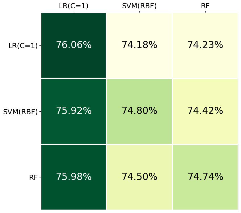
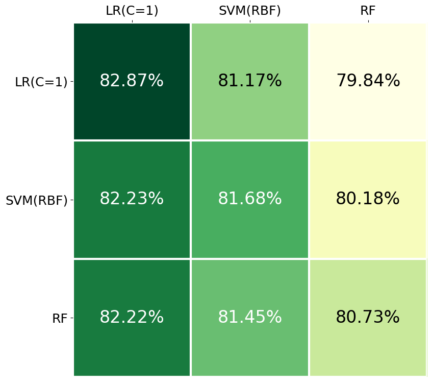
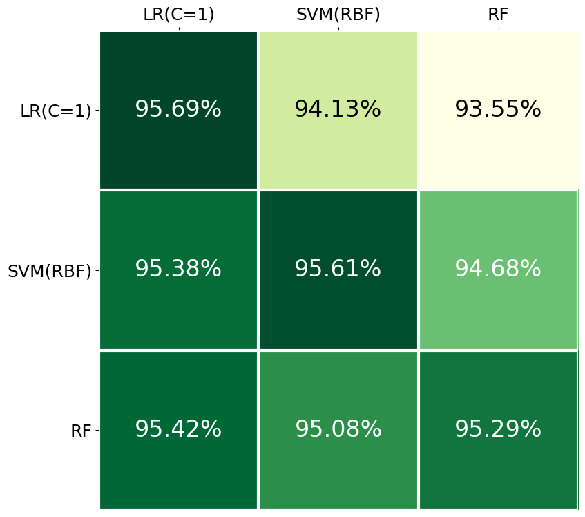
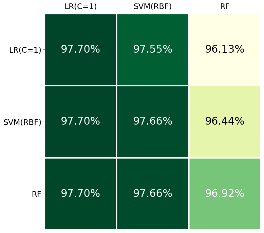
Figure 8: Mean AUBC of query-oriented model and task-oriented model on group 1. (Compatible LRs achieve best results.): Diabetes (top-left), Mammographic (top-right), Gcloudub (bottom-left), and Twonorm (bottom-right).

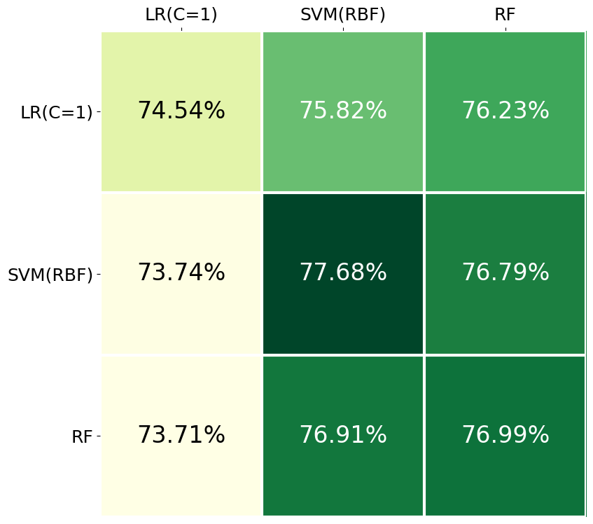
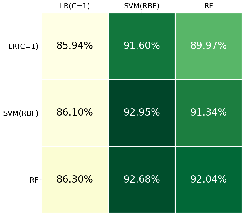
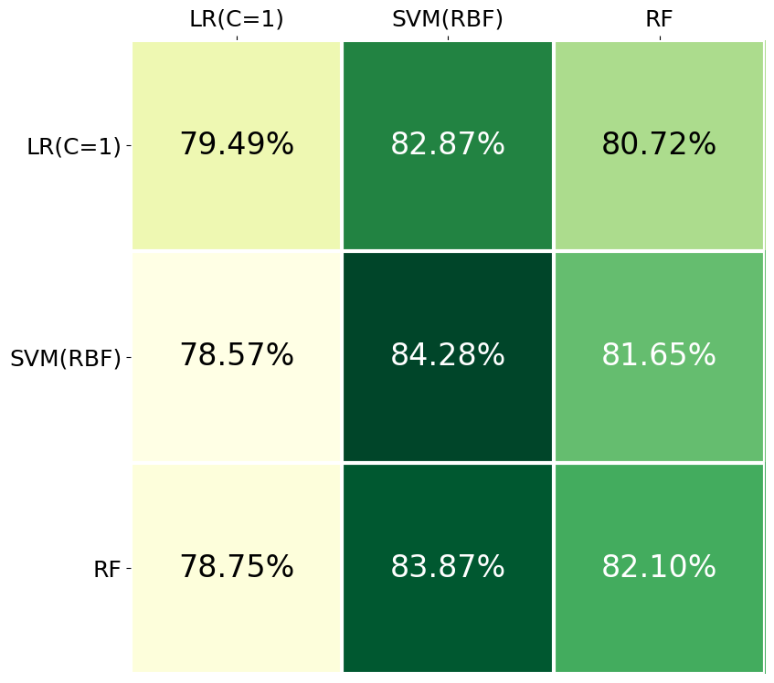
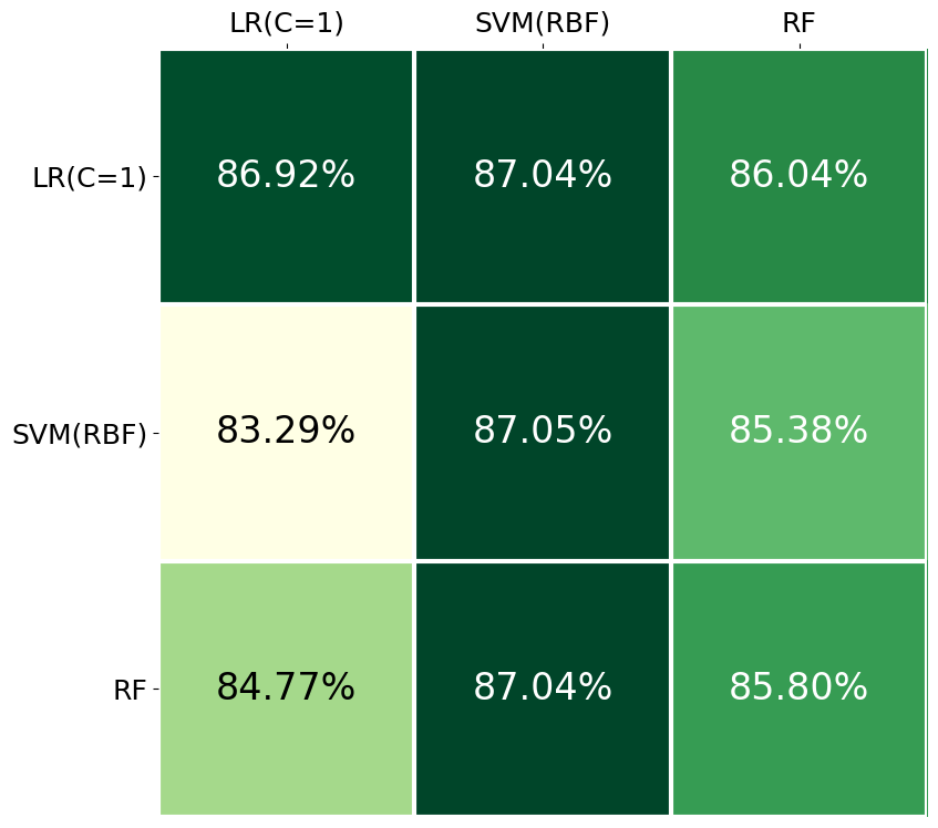
Figure 9: Mean AUBC of query-oriented model and task-oriented model on group 2. (Compatible SVMs achieve best results.): Sonar (top-left), Ionosphere (top-right), Clean1 (middle-left), Tic (middle-left), Gcloudb (bottom-left), and Ringnorm (bottom-right).

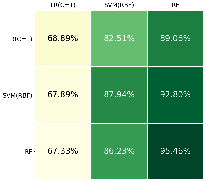
Figure 10: Mean AUBC of query-oriented model and task-oriented model on group 3. (Compatible RFs achieve best results.): Parkinsons (top-left), Breast (top-right), Australian (bottom-left), and Ex8a (bottom-right).

Figure 12: Mean AUBC of query-oriented model and task-oriented model on group 5. (Non-Compatible models achieve best results.): Heart (top-left), Splice (top-right), Checkerboard (bottom-left), and Banana (bottom-right).

References

- Ash et al. [2019] J. T. Ash, C. Zhang, A. Krishnamurthy, J. Langford, and A. Agarwal. Deep batch active learning by diverse, uncertain gradient lower bounds. arXiv preprint arXiv:1906.03671, 2019.
- Beck et al. [2021] N. Beck, D. Sivasubramanian, A. Dani, G. Ramakrishnan, and R. Iyer. Effective evaluation of deep active learning on image classification tasks. arXiv preprint arXiv:2106.15324, 2021.
- Bommaraveni et al. [2019] S. Bommaraveni, T. X. Vu, S. Vuppala, S. Chatzinotas, and B. Ottersten. Active content popularity learning via query-by-committee for edge caching. In 2019 53rd Asilomar Conference on Signals, Systems, and Computers, pages 301–305. IEEE, 2019.
- Brust et al. [2018] C.-A. Brust, C. Käding, and J. Denzler. Active learning for deep object detection. arXiv preprint arXiv:1809.09875, 2018.
- Cai et al. [2016] W. Cai, M. Zhang, and Y. Zhang. Batch mode active learning for regression with expected model change. IEEE transactions on neural networks and learning systems, 28(7):1668–1681, 2016.
- Cawley [2011] G. C. Cawley. Baseline methods for active learning. In Active Learning and Experimental Design workshop In conjunction with AISTATS 2010, pages 47–57. JMLR Workshop and Conference Proceedings, 2011.
- Chang and Lin [2011] C.-C. Chang and C.-J. Lin. LIBSVM: A library for support vector machines. ACM Transactions on Intelligent Systems and Technology, 2:27:1–27:27, 2011. Software available at http://www.csie.ntu.edu.tw/c̃jlin/libsvm.
- Chattopadhyay et al. [2012] R. Chattopadhyay, Z. Wang, W. Fan, I. Davidson, S. Panchanathan, and J. Ye. Batch mode active sampling based on marginal probability distribution matching. KDD : proceedings. International Conference on Knowledge Discovery & Data Mining, 2012:741–749, 2012.
- Cheng and Dong [2021] F. Cheng and J. Dong. Data-driven online detection of tip wear in tip-based nanomachining using incremental adaptive support vector machine. Journal of Manufacturing Processes, 69:412–421, 2021.
- Dasgupta and Hsu [2008] S. Dasgupta and D. Hsu. Hierarchical sampling for active learning. In Proceedings of the 25th international conference on Machine learning, pages 208–215, 2008.
- Demir et al. [2015] E. Demir, Z. Cataltepe, U. Ekmekci, M. Budnik, and L. Besacier. Unsupervised Active Learning For Video Annotation. In ICML Active Learning Workshop 2015, Lille, France, July 2015. URL https://hal.science/hal-01350092.
- Deng et al. [2009] J. Deng, W. Dong, R. Socher, L.-J. Li, K. Li, and L. Fei-Fei. Imagenet: A large-scale hierarchical image database. In 2009 IEEE Conference on Computer Vision and Pattern Recognition, pages 248–255, 2009. doi: 10.1109/CVPR.2009.5206848.
- Desreumaux and Lemaire [2020] L. Desreumaux and V. Lemaire. Learning active learning at the crossroads? evaluation and discussion. arXiv e-prints, art. arXiv:2012.09631, Dec. 2020.
- Diamond and Boyd [2016] S. Diamond and S. Boyd. CVXPY: A Python-embedded modeling language for convex optimization. Journal of Machine Learning Research, 17(83):1–5, 2016.
- Dong [2021] S. Dong. Multi class svm algorithm with active learning for network traffic classification. Expert Systems with Applications, 176:114885, 2021.
- Dua and Graff [2017] D. Dua and C. Graff. UCI machine learning repository, 2017. URL http://archive.ics.uci.edu/ml.
- Ebert et al. [2012] S. Ebert, M. Fritz, and B. Schiele. Ralf: A reinforced active learning formulation for object class recognition. In 2012 IEEE Conference on Computer Vision and Pattern Recognition, pages 3626–3633, 2012. doi: 10.1109/CVPR.2012.6248108.
- Goyal et al. [2021] P. Goyal, Q. Duval, J. Reizenstein, M. Leavitt, M. Xu, B. Lefaudeux, M. Singh, V. Reis, M. Caron, P. Bojanowski, A. Joulin, and I. Misra. Vissl. https://github.com/facebookresearch/vissl, 2021.
- Grigorescu et al. [2020] S. Grigorescu, B. Trasnea, T. Cocias, and G. Macesanu. A survey of deep learning techniques for autonomous driving. Journal of Field Robotics, 37(3):362–386, 2020.
- Guyon et al. [2010] I. Guyon, G. Cawley, G. Dror, and V. Lemaire. Design and analysis of the wcci 2010 active learning challenge. In The 2010 International Joint Conference on Neural Networks (IJCNN), pages 1–8, 2010. doi: 10.1109/IJCNN.2010.5596506.
- Guyon et al. [2011] I. Guyon, G. C. Cawley, G. Dror, and V. Lemaire. Results of the active learning challenge. In I. Guyon, G. Cawley, G. Dror, V. Lemaire, and A. Statnikov, editors, Active Learning and Experimental Design workshop In conjunction with AISTATS 2010, volume 16 of Proceedings of Machine Learning Research, pages 19–45, Sardinia, Italy, 16 May 2011. PMLR. URL https://proceedings.mlr.press/v16/guyon11a.html.
- Ji et al. [2023] Y. Ji, D. Kaestner, O. Wirth, and C. Wressnegger. Randomness is the root of all evil: More reliable evaluation of deep active learning. In 2023 IEEE/CVF Winter Conference on Applications of Computer Vision (WACV), pages 3932–3941, 2023. doi: 10.1109/WACV56688.2023.00393.
- Karamcheti et al. [2021] S. Karamcheti, R. Krishna, L. Fei-Fei, and C. Manning. Mind your outliers! investigating the negative impact of outliers on active learning for visual question answering. In Proceedings of the 59th Annual Meeting of the Association for Computational Linguistics and the 11th International Joint Conference on Natural Language Processing (Volume 1: Long Papers), pages 7265–7281, Online, Aug. 2021. Association for Computational Linguistics. doi: 10.18653/v1/2021.acl-long.564. URL https://aclanthology.org/2021.acl-long.564.
- Kishaan et al. [2020] J. Kishaan, M. Muthuraja, D. Nair, and P.-G. Plöger. Using active learning for assisted short answer grading. 2020.
- Konyushkova et al. [2017] K. Konyushkova, R. Sznitman, and P. Fua. Learning active learning from data. In I. Guyon, U. V. Luxburg, S. Bengio, H. Wallach, R. Fergus, S. Vishwanathan, and R. Garnett, editors, Advances in Neural Information Processing Systems, volume 30. Curran Associates, Inc., 2017. URL https://proceedings.neurips.cc/paper/2017/file/8ca8da41fe1ebc8d3ca31dc14f5fc56c-Paper.pdf.
- Kottke et al. [2017] D. Kottke, A. Calma, D. Huseljic, G. Krempl, B. Sick, et al. Challenges of reliable, realistic and comparable active learning evaluation. In Proceedings of the Workshop and Tutorial on Interactive Adaptive Learning, pages 2–14, 2017.
- Kremer et al. [2014] J. Kremer, K. Steenstrup Pedersen, and C. Igel. Active learning with support vector machines. Wiley Int. Rev. Data Min. and Knowl. Disc., 4(4):313–326, jul 2014. ISSN 1942-4787. doi: 10.1002/widm.1132. URL https://doi.org/10.1002/widm.1132.
- Krizhevsky et al. [2017] A. Krizhevsky, I. Sutskever, and G. E. Hinton. Imagenet classification with deep convolutional neural networks. Communications of the ACM, 60(6):84–90, 2017.
- Li et al. [2015] C.-L. Li, C.-S. Ferng, and H.-T. Lin. Active learning using hint information. Neural computation, 27(8):1738–1765, 2015.
- Litjens et al. [2017] G. Litjens, T. Kooi, B. E. Bejnordi, A. A. A. Setio, F. Ciompi, M. Ghafoorian, J. A. Van Der Laak, B. Van Ginneken, and C. I. Sánchez. A survey on deep learning in medical image analysis. Medical image analysis, 42:60–88, 2017.
- Logan et al. [2022] Y.-y. Logan, M. Prabhushankar, and G. AlRegib. Decal: Deployable clinical active learning. arXiv preprint arXiv:2206.10120, 2022.
- Lu et al. [2023] P.-Y. Lu, C.-L. Li, and H.-T. Lin. A more robust baseline for active learning by injecting randomness to uncertainty sampling. In Proceedings of the AI and HCI Workshop @ ICML, July 2023.
- Lüth et al. [2023] C. T. Lüth, T. J. Bungert, L. Klein, and P. F. Jaeger. Toward realistic evaluation of deep active learning algorithms in image classification. arXiv preprint arXiv:2301.10625, 2023.
- Munjal et al. [2022] P. Munjal, N. Hayat, M. Hayat, J. Sourati, and S. Khan. Towards robust and reproducible active learning using neural networks. In Proceedings of the IEEE/CVF Conference on Computer Vision and Pattern Recognition, pages 223–232, 2022.
- Mussmann and Liang [2018] S. Mussmann and P. Liang. On the relationship between data efficiency and error for uncertainty sampling. In International Conference on Machine Learning, pages 3674–3682. PMLR, 2018.
- Mussmann et al. [2022] S. Mussmann, J. Reisler, D. Tsai, E. Mousavi, S. O’Brien, and M. Goldszmidt. Active learning with expected error reduction. arXiv preprint arXiv:2211.09283, 2022.
- Narayanan et al. [2020] S. D. Narayanan, A. Agnihotri, and N. Batra. Active learning for air quality station deployment. 2020.
- Nath et al. [2020] V. Nath, D. Yang, B. A. Landman, D. Xu, and H. R. Roth. Diminishing uncertainty within the training pool: Active learning for medical image segmentation. IEEE Transactions on Medical Imaging, 40:2534–2547, 2020.
- Pedregosa et al. [2011] F. Pedregosa, G. Varoquaux, A. Gramfort, V. Michel, B. Thirion, O. Grisel, M. Blondel, P. Prettenhofer, R. Weiss, V. Dubourg, J. Vanderplas, A. Passos, D. Cournapeau, M. Brucher, M. Perrot, and E. Duchesnay. Scikit-learn: Machine learning in Python. Journal of Machine Learning Research, 12:2825–2830, 2011.
- Sass et al. [2022] R. Sass, E. Bergman, A. Biedenkapp, F. Hutter, and M. Lindauer. Deepcave: An interactive analysis tool for automated machine learning, 2022. URL https://arxiv.org/abs/2206.03493.
- Sener and Savarese [2018] O. Sener and S. Savarese. Active learning for convolutional neural networks: A core-set approach. In International Conference on Learning Representations, 2018. URL https://openreview.net/forum?id=H1aIuk-RW.
- Settles [2012] B. Settles. Active Learning, volume 6. Springer, 7 2012. doi: 10.2200/S00429ED1V01Y201207AIM018. URL https://www.morganclaypool.com/doi/abs/10.2200/S00429ED1V01Y201207AIM018?ai=1ge&mi=6e3g68&af=R.
- Seung et al. [1992] H. S. Seung, M. Opper, and H. Sompolinsky. Query by committee. In Proceedings of the fifth annual workshop on Computational learning theory, pages 287–294, 1992.
- Shui et al. [2020] C. Shui, F. Zhou, C. Gagné, and B. Wang. Deep active learning: Unified and principled method for query and training. In International Conference on Artificial Intelligence and Statistics, pages 1308–1318. PMLR, 2020.
- Sinha et al. [2019] S. Sinha, S. Ebrahimi, and T. Darrell. Variational adversarial active learning. In Proceedings of the IEEE/CVF International Conference on Computer Vision, pages 5972–5981, 2019.
- Tang et al. [2019] Y.-P. Tang, G.-X. Li, and S.-J. Huang. ALiPy: Active learning in python. Technical report, Nanjing University of Aeronautics and Astronautics, 1 2019. URL https://github.com/NUAA-AL/ALiPy. available as arXiv preprint https://arxiv.org/abs/1901.03802.
- Tifrea et al. [2022] A. Tifrea, J. Clarysse, and F. Yang. Uniform versus uncertainty sampling: When being active is less efficient than staying passive. arXiv preprint arXiv:2212.00772, 2022.
- Trittenbach et al. [2021] H. Trittenbach, A. Englhardt, and K. Böhm. An overview and a benchmark of active learning for outlier detection with one-class classifiers. Expert Systems with Applications, 168:114372, 2021. ISSN 0957-4174. doi: https://doi.org/10.1016/j.eswa.2020.114372. URL https://www.sciencedirect.com/science/article/pii/S0957417420310496.
- Vandoni et al. [2019] J. Vandoni, E. Aldea, and S. Le Hégarat-Mascle. Evidential query-by-committee active learning for pedestrian detection in high-density crowds. International Journal of Approximate Reasoning, 104:166–184, 2019.
- Wang et al. [2022a] X. Wang, Y. Li, J. Chen, J. Yang, et al. Enhancing personalized recommendation by transductive support vector machine and active learning. Security and Communication Networks, 2022, 2022a.
- Wang et al. [2022b] Y. Wang, H. Chen, Y. Fan, W. SUN, R. Tao, W. Hou, R. Wang, L. Yang, Z. Zhou, L.-Z. Guo, H. Qi, Z. Wu, Y.-F. Li, S. Nakamura, W. Ye, M. Savvides, B. Raj, T. Shinozaki, B. Schiele, J. Wang, X. Xie, and Y. Zhang. USB: A unified semi-supervised learning benchmark for classification. In Thirty-sixth Conference on Neural Information Processing Systems Datasets and Benchmarks Track, 2022b. URL https://openreview.net/forum?id=QeuwINa96C.
- Wang and Ye [2015] Z. Wang and J. Ye. Querying discriminative and representative samples for batch mode active learning. ACM Trans. Knowl. Discov. Data, 9(3), feb 2015. ISSN 1556-4681. doi: 10.1145/2700408. URL https://doi.org/10.1145/2700408.
- Wu et al. [2019] D. Wu, C.-T. Lin, and J. Huang. Active learning for regression using greedy sampling. Information Sciences, 474:90–105, 2019.
- Yang and Loog [2018] Y. Yang and M. Loog. A benchmark and comparison of active learning for logistic regression. Pattern Recognition, 83:401–415, 2018. ISSN 0031-3203. doi: https://doi.org/10.1016/j.patcog.2018.06.004. URL https://www.sciencedirect.com/science/article/pii/S0031320318302140.
- Yang et al. [2015] Y. Yang, Z. Ma, F. Nie, X. Chang, and A. G. Hauptmann. Multi-class active learning by uncertainty sampling with diversity maximization. International Journal of Computer Vision, 113:113–127, 2015.
- Yang et al. [2017] Y.-Y. Yang, S.-C. Lee, Y.-A. Chung, T.-E. Wu, S.-A. Chen, and H.-T. Lin. libact: Pool-based active learning in python. Technical report, National Taiwan University, 10 2017. URL https://github.com/ntucllab/libact. available as arXiv preprint https://arxiv.org/abs/1710.00379.
- Yilei “Dolee” Yang [2017] r. Yilei “Dolee” Yang. Active learning playground. https://github.com/google/active-learning, 2017. URL https://github.com/google/active-learning.
- Yoo and Kweon [2019] D. Yoo and I. S. Kweon. Learning loss for active learning. In Proceedings of the IEEE/CVF conference on computer vision and pattern recognition, pages 93–102, 2019.
- Yuan et al. [2021] T. Yuan, F. Wan, M. Fu, J. Liu, S. Xu, X. Ji, and Q. Ye. Multiple instance active learning for object detection. In Proceedings of the IEEE/CVF Conference on Computer Vision and Pattern Recognition, pages 5330–5339, 2021.
- Zhan et al. [2021] X. Zhan, H. Liu, Q. Li, and A. B. Chan. A comparative survey: Benchmarking for pool-based active learning. In Z.-H. Zhou, editor, Proceedings of the Thirtieth International Joint Conference on Artificial Intelligence, IJCAI-21, pages 4679–4686. International Joint Conferences on Artificial Intelligence Organization, 8 2021. doi: 10.24963/ijcai.2021/634. URL https://doi.org/10.24963/ijcai.2021/634. Survey Track.
- Zhan et al. [2022] X. Zhan, Q. Wang, K.-h. Huang, H. Xiong, D. Dou, and A. B. Chan. A comparative survey of deep active learning. arXiv preprint arXiv:2203.13450, 2022.
- Zhang et al. [2020] H. Zhang, S. Ravi, and I. Davidson. A graph-based approach for active learning in regression. In Proceedings of the 2020 SIAM International Conference on Data Mining, pages 280–288. SIAM, 2020.
- Zhang et al. [2021] J. Zhang, Y. Yu, Y. Li, Y. Wang, Y. Yang, M. Yang, and A. Ratner. WRENCH: A comprehensive benchmark for weak supervision. In Thirty-fifth Conference on Neural Information Processing Systems Datasets and Benchmarks Track, 2021. URL https://openreview.net/forum?id=Q9SKS5k8io.
- Zhang et al. [2022] Z. Zhang, E. Strubell, and E. Hovy. A survey of active learning for natural language processing. arXiv preprint arXiv:2210.10109, 2022.