Active Representation Learning for General Task Space with Applications in Robotics

Abstract

Representation learning based on multi-task pretraining has become a powerful approach in many domains. In particular, task-aware representation learning aims to learn an optimal representation for a specific target task by sampling data from a set of source tasks, while task-agnostic representation learning seeks to learn a universal representation for a class of tasks. In this paper, we propose a general and versatile algorithmic and theoretic framework for active representation learning, where the learner optimally chooses which source tasks to sample from. This framework, along with a tractable meta algorithm, allows most arbitrary target and source task spaces (from discrete to continuous), covers both task-aware and task-agnostic settings, and is compatible with deep representation learning practices. We provide several instantiations under this framework, from bilinear and feature-based nonlinear to general nonlinear cases. In the bilinear case, by leveraging the non-uniform spectrum of the task representation and the calibrated source-target relevance, we prove that the sample complexity to achieve $\varepsilon$-excess risk on target scales with $(k^{*})^{2}\|v^{*}\|_{2}^{2}\varepsilon^{-2}$ where $k^{*}$ is the effective dimension of the target and $\|v^{*}\|_{2}^{2}\in(0,1]$ represents the connection between source and target space. Compared to the passive one, this can save up to $\frac{1}{d_{W}}$ of sample complexity, where $d_{W}$ is the task space dimension. Finally, we demonstrate different instantiations of our meta algorithm in synthetic datasets and robotics problems, from pendulum simulations to real-world drone flight datasets. On average, our algorithms outperform baselines by $20\%-70\%$.

1 Introduction

Recently, few-shot machine learning has enjoyed significant attention and has become increasingly critical due to its ability to derive meaningful insights for target tasks that have minimal data, a scenario commonly encountered in real-world applications. This issue is especially prevalent in robotics where data collection and training data is prohibitive to collect or even non-reproducible (e.g., drone flying with complex aerodynamics [1] or legged robots on challenging terrains [2]). One promising approach to leveraging the copious amount of data from a variety of other sources is multi-task learning, which is based on a key observation that different tasks may share a common low-dimensional representation. This process starts by pretraining a representation on source tasks and then fine-tuning the learned representation using a limited amount of target data ([3, 4, 5, 6, 7]).

In conventional supervised learning tasks, accessing a large amount of source data for multi-task representation learning may be easy, but processing and training on all that data can be costly. In real-world physical systems like robotics, this challenge is further amplified by two factors: (1) switching between different tasks or environments is often significantly more expensive (e.g., reset giant wind tunnels for drones [7]); (2) there are infinitely many environments to select from (i.e., environmental conditions are continuous physical parameters like wind speed). Therefore, it is crucial to minimize not only the number of samples, but the number of sampled source tasks, while still achieving the desired performance on the target task. Intuitively, not all source tasks are equally informative for learning a universally good representation or a target-specific representation. This is because source tasks can have a large degree of redundancy or be scarce in other parts of the task space. In line with this observation, Chen et al. [8] provided the first provable active representation learning method that improves training efficiency and reduces the cost of processing source data by prioritizing certain tasks during training with theoretical guarantees. On the other hand, many existing works [9, 10, 11, 12, 13] prove that it is statistically possible to learn a universally good representation by randomly sampling source tasks (i.e., the passive learning setting).

The previous theoretical work of [8] on active multi-task representation learning has three main limitations. First, it only focuses on a finite number of discrete tasks, treating each source independently, and therefore fails to leverage the connection between each task. This could be sub-optimal in many real-world systems like robotics for two reasons: (1) there are often infinitely many sources to sample from (e.g., wind speed for drones); (2) task spaces are often highly correlated (e.g., perturbing the wind speed will not drastically change the aerodynamics). In our paper, by considering a more general setting where tasks are parameterized in a vector space ${\mathcal{W}}$, we can more effectively leverage similarities between tasks compared to treating them as simply discrete and different. Secondly, the previous work only considers a single target, while we propose an algorithm that works for an arbitrary target space and distribution. This is particularly useful when the testing scenario is time-variant. Thirdly, we also consider the task-agnostic setting by selecting $\mathcal{O}(k)$ representative tasks among the $d_{W}$ high dimension task space, where $k\ll d_{W}$ is the dimension of the shared representation. Although this result does not improve the total source sample complexity compared to the passive learning result in the bilinear setting [12], it reduces the number of tasks used in the training and therefore implicitly facilitates the training process.

In addition to those theoretical contributions, we extend our proposed algorithmic framework beyond a pure bilinear representation function, including the known nonlinear feature operator with unknown linear representation (e.g., random features with unknown coefficients), and the totally unknown nonlinear representation (e.g., deep neural network representation). While some prior works have considered nonlinear representations [9, 10, 14, 13] in passive learning, the studies in active learning are relatively limited [8]. All of these works only consider non-linearity regarding the input, rather than the task parameter. In this paper, we model task-parameter-wise non-linearity and show its effectiveness in experiments. Note that it particularly matters for task selections because the mapping from the representation space to task parameters to is no longer linear.

1.1 Summery of contributions

• We propose the first generic active representation learning framework that admits any arbitrary source and target task space. This result greatly generalizes previous works where tasks lie in the discrete space and only a single target is allowed. To show its flexibility, we also provide discussions on how our framework can accommodate various supervised training oracles and optimal design oracles. (Section 3)

• We provide theoretical guarantees under a benign setting, where inputs are i.i.d. and a unit ball is contained in the overall task space, as a compliment to the previous work where tasks lie on the vertices of the whole space. In the target-aware setting, to identify an $\varepsilon$-good model our method requires a sample complexity of $\widetilde{\mathcal{O}}(kd_{X}(k^{*})^{2}\|v^{*}\|_{2}^{2}\min\{k^{*},\kappa^{2}\}\varepsilon^{-2})$ where $k^{*}$ is the effective dimension of the target, $\kappa$ is the conditional number of representation matrix, and $\|v^{*}\|_{2}^{2}\in(0,1]$ represents the connection between source and target space that will be specified in the main paper. Compared to passive learning, our result saves up to a factor of $\frac{k^{2}}{d_{W}}$ in the sample complexity when targets are uniformly spread over the $k$-dim space and up to $\frac{1}{d_{W}}$ when targets are highly concentrated. Our results further indicate the necessity of considering the continuous space by showing that directly applying the previous algorithm onto some discretized sources in the continuous space (e.g., orthonormal basis) can lead to worse result. Finally, ignoring the tasks used in the warm-up phases, in which only a few samples are required, both the target-aware and the target-agnostic cases can save up to $\widetilde{\mathcal{O}}(k^{*}+k)$ number of tasks compared to the passive one which usually requires $d_{W}$ number of tasks. (Section 4)

• We provide comprehensive experimental results under different instantiations beyond the benign theoretical setting, studying synthetic and real-world scenarios: 1) For the synthetic data setting in a continuous space, we provide results for pure linear, known nonlinear feature operator $\psi_{X}$ and unknown nonlinear representation $\phi_{X}$. Our target-aware active learning (AL) approach shows up to a significant budget saving (up to $68\%$) compared to the passive approach and the target-agnostic AL approach also shows an advantage in the first two cases. 2) In a pendulum simulation with continuous task space, we provide the results for known nonlinear feature operator $\psi_{X}$ and $\psi_{W}$ and show that our target-aware AL approach has up to $20\%$ loss reduction compared to the passive one, which also translates to better nonlinear control performance. 3) Finally, in the real-world drone dataset with a discrete task space, we provide results for unknown linear and nonlinear representation $\phi_{X}$ and show that our target-aware AL approach converges much faster than the passive one. (Section 5)

2 Preliminary

Multi-task (or multi-environments).

Each task or environment is parameterized by a known vector $w\in\mathbb{R}^{d_{W}}$. We denote the source and target task parameter space as ${\mathcal{W}}_{\text{source}}\subset\mathbb{R}^{d_{W}},{\mathcal{W}}_{\text{target}}\subset\mathbb{R}^{d_{W}}$. These spaces need not be the same (e.g., they could be different sub-spaces). In the discrete case, we set $w$ as a one-hot encoded vector and therefore we have in total $d_{W}$ number of candidate tasks while in the continuous space, there exist infinitely many tasks. For convenience, we also use $w$ as the subscript to index certain tasks. In addition, we use $\nu_{\text{source}}\in\Delta({\mathcal{W}}_{\text{source}}),\nu_{\text{target}}\in\Delta({\mathcal{W}}_{\text{target}})$ to denote the task distribution for the sources and targets.

Data generation.

Let ${\mathcal{X}}\in\mathbb{R}^{d_{X}}$ be the input space. We first assume there exists some known feature/augmentation operator $\psi_{X}:{\mathcal{X}}\to\mathbb{R}^{d_{\psi_{X}}\geq d_{W}},\psi_{W}:{\mathcal{W}}\to\mathbb{R}^{d_{\psi_{W}}\geq d_{W}}$, that can be some non-linear operator that lifts $w,x$ to some higher dimensional space (e.g., random Fourier features [15]). Notice that the existence of non-identical $\psi$ indicates the features are not pairwise independent and the design space of ${\mathcal{W}}_{\text{source}}$ is not benign (e.g., non-convex), which adds extra difficulty to this problem.

Then we assume there exists some unknown underlying representation function $\phi_{X}:\psi({\mathcal{X}})\rightarrow{\mathcal{R}}$ which maps the augmented input space $\psi({\mathcal{X}})$ to a shared representation space ${\mathcal{R}}\in\mathbb{R}^{k}$ where $k\ll d_{\psi_{X}},k\leq d_{\psi_{W}}$, and its task counterparts $\phi_{W}:\psi({\mathcal{W}})\rightarrow{\mathcal{R}}$ which maps parameterized task space to the feature space. Here the representation functions are restricted to be in some function classes $\Phi$, e.g., linear functions, deep neural networks, etc.

In this paper, we further assume that $\phi_{W}$ is a linear function $B_{W}\in\mathbb{R}^{k\times d_{\psi_{W}}}$. To be more specific, for any fixed task $w$, we assume each sample $(x,y)\sim\nu_{w}$ satisfies

$$y=\phi_{X}(\psi_{X}(x))^{\top}B_{W}\psi_{W}(w)+\xi,\quad\xi\sim\mathcal{N}(0,\sigma^{2})$$ (1)

For convenience, we denote $Z_{w}$ as the collection of $n_{w}$ sampled data $(x_{w}^{1},y_{w}^{1}),...,(x_{w}^{n_{w}},y_{w}^{n_{w}})\sim\mu_{w}$. We note that when $\psi_{X},\psi_{W}$ is identity and $\phi_{X}$ is linear, this is reduced to standard linear setting in many previous papers [9, 11, 12, 8].

The task diversity assumption.

There exists some distribution $p\in\Delta({\mathcal{W}}_{\text{source}})$ that $\mathbb{E}_{w\sim p}\lambda_{\min}(B_{W}\psi_{W}(w)\psi_{W}(w)^{\top}B_{W}^{\top})>0$, which suggests the source tasks are diverse enough to learn the representation.

Data collection protocol.

We assume there exists some i.i.d. data sampling oracle given the environment and the budget. To learn a proper representation, we are allowed access to an unlimited $n_{\text{source}}$ number of data from source tasks during the learning process by using such an oracle. Then at the end of the algorithm, we are given a few-shot of mix target data $Z_{\text{target}}=\{Z_{w}\}_{w\sim\nu_{\text{target}}}$ which is used for fine-tuning based on learned representation $\hat{\phi}_{X}$. Denote $n_{\text{target}}$ as the number of data points in $Z_{\text{target}}$.

Data collection protocol for target-aware setting.

When the target task is not a singleton, we additionally assume a few-shot of known environment target data $\dot{Z}_{\text{target}}:=\{Z_{w},w\}_{w\in\dot{W}_{\text{target}}}$, where $|\dot{W}_{\text{target}}|=\text{dim}({\mathcal{W}}_{\text{target}})$ and $\dot{W}_{\text{target}}=\{\operatorname*{arg\,max}_{W\in{\mathcal{W}}_{\text{target}}}\lambda_{\min}(WW^{\top})\}$. Again denote $\dot{n}_{\text{target}}$ as the number of data points in $\dot{Z}_{\text{target}}$, we have $\dot{n}_{\text{target}}\approx n_{\text{target}}^{2/3}\ll n_{\text{source}}$.

Remark 2.1.

Here $|\dot{W}_{\text{target}}|$ represents vectors that can cover every directions of ${\mathcal{W}}_{\text{target}}$ space. This extra $\dot{Z}_{\text{target}}$ requirement comes from the non-linearity of $l_{2}$ loss and the need to learn the relationship between sources and targets. We want to emphasize that such an assumption implicitly exists in previous active representation learning [8] since $\dot{Z}_{\text{target}}=Z_{\text{target}}$ in their single target setting. Nevertheless, in a passive learning setting, only mixed $Z_{\text{target}}$ is required since no source selection process involves. Whether such a requirement is necessary for target-aware active learning remains an open problem.

Other notations.

Let $e_{i}$ to be one-hot vector with $1$ at $i$-th coordinates and let $\epsilon_{i}=2^{-i}$.

2.1 Goals

Expected excess risk.

For any target task space ${\mathcal{W}}_{\text{target}}$ and its distribution $\nu_{\text{target}}$ over the space, as well as a few-shot examples as stated in section 2, our goal is to minimize the expected excess risk with our estimated $\hat{\phi}_{X}$

$${\textsc{er}}(\hat{\phi}_{X},\nu_{\text{target}})=\mathbb{E}_{w_{0}\sim\nu_{\text{target}}}\mathbb{E}_{(x,y)\sim\nu_{w_{0}}}\|\hat{\phi}_{X}(\psi_{X}(x))^{\top}\hat{w}_{\text{avg}}-y\|_{2}$$

where $\hat{w}_{\text{avg}}=\operatorname*{arg\,min}_{w}\sum_{(x,y)\in Z_{\text{target}}}\|\hat{\phi}_{X}(\psi_{X}(x))w-y\|_{2}$, which average model estimation that captures the data behavior under the expected target distribution. Note that the ${\mathcal{W}}_{\text{target}},\nu_{\text{target}}$ are given in advance in the target-aware setting.

The number of tasks.

Another side goal is to save the number of long-term tasks we are going to sample during the learning process. Since a uniform exploration over $d_{W}^{\text{source}}$-dimension is unavoidable during the warm-up stage, we define long-term task number as

$$\left\lvert\left\{w\in{\mathcal{W}}_{\text{source}}\mid\ n_{w}\geq\tilde{\Omega}(\varepsilon^{-\alpha})\right\}\right\rvert$$

where $\alpha$ is some arbitrary exponent and $\varepsilon$ is the target accuracy and $n_{w}$ is number of samples sampled from task $w$ as defined above.

3 A general framework

Algorithm 1 Active multi-task representation learning (general templates)

1:  Inputs: Candidate source set ${\mathcal{W}}_{\text{source}}$. Classes of candidate representation function $\Phi_{X},\Phi_{W}$ and the known feature operator $\psi_{X},\psi_{W}$.

2:  [Target-aware only] Inputs: Target set ${\mathcal{W}}_{\text{target}}$ and distribution $\nu_{\text{target}}$. Few-shot sample $\dot{Z}_{\text{target}}$ as defined in the preliminary.

3:  Stage 1: Coarse exploration. (Warm-up stage)

4:  Set initial sampling distribution $q_{0}=g(\psi_{W},I_{d_{\psi_{W}}})$ where $g$ is defined in Eqn. 2

5:  Set $n_{0}\approx\text{poly}(d_{\psi_{X}},k)+\text{poly}(d_{\psi_{W}},k)$. Collect $n_{0}q_{0}(w)$ data for each task denoted as $\{Z_{w}\}_{w|q_{0}(w)\neq 0}$ and update $\hat{\phi}_{X}\leftarrow{\mathcal{O}}_{\text{offline 0}}^{X}(\{Z_{w}\}_{w|q_{0}(w)\neq 0},\psi_{X})$ and $\hat{B}_{W}\leftarrow{\mathcal{O}}_{\text{offline}}^{W}(\{Z_{w}\}_{w|q_{0}(w)\neq 0},\hat{\phi}_{X})$

6:  for $j=1,2,3,\ldots$ do

7:     Stage 2: Fine target-agnostic exploration (Directly choose $q_{1}^{j}=q_{0}$ when $k=\Theta(d_{W})$)

8:     Compute the exploration sampling distribution $q_{1}^{j}=g(\hat{B}_{W}\circ\psi_{W},I_{k})$

9:     $n_{1}^{j}\approx\text{poly}(d_{\psi_{X}},k)\epsilon_{j}^{-\frac{4}{3}}$. Collect $n_{1}^{j}q_{1}^{j}(w)$ data for each task denoted as $\{Z_{w}\}_{w|q(w)\neq 0}$ and update $\hat{\phi}_{X}\leftarrow{\mathcal{O}}_{\text{offline 1}}^{X}(\{Z_{w}\}_{w|q_{1}^{j}(w)\neq 0},\psi_{X})$ and $\hat{B}_{W}\leftarrow{\mathcal{O}}_{\text{offline}}^{W}(\{Z_{w}\}_{w|q_{1}^{j}(w)\neq 0},\dot{Z}_{\text{target}},\hat{\phi}_{X})$

10:     [Target-aware only] Stage 3: Fine target-aware exploration

11:     Compute the exploitation sampling distribution $q_{2}^{j}=g(\hat{B}_{W}\circ\psi_{W},\Sigma_{\text{regu}})$ where $\Sigma_{\text{regu}}$ is the regularized version of $\hat{B}_{W}(\mathbb{E}_{w_{0}\sim\nu_{0}}w_{0}w_{0}^{\top})\hat{B}_{W}^{\top}$ after clipping out insignificant eigenvalues.

12:     Set $n_{2}^{j}\approx\text{poly}(d_{\psi_{X}},k)\epsilon_{j}^{-2}$. Collect $n_{2}^{j}q_{2}^{j}(w)$ data for each task denoted as $\{Z_{w}\}_{w|q_{2}^{j}(w)\neq 0}$ and update $\hat{\phi}_{X}\leftarrow{\mathcal{O}}_{\text{offline 3}}^{X}(\{Z_{w}\}_{w|q_{1}^{j}(w)\neq 0\text{ and }q_{2}^{j}(w)\neq 0},\psi_{X})$.

13:  end for

14:  Return $\hat{\phi}_{X}$

Our algorithm 1 iteratively estimates the shared representation $\hat{\phi}_{X},\hat{B}_{W}$ and the next target relevant source tasks which the learner should sample from by solving several optimal design oracles

$$g(f,A)=\min_{q\in\Delta({\mathcal{W}}_{source})}\lambda_{\max}\left((\int q(w)f(w)f(w)^{\top})^{-1}A\right)$$ (2)

This exploration and exploitation (target-aware exploration here) trade-off is inspired by the classical $\epsilon$-greedy strategy, but the key difficulty in our work is to combine that with multi-task representation learning and different optimal design problems. The algorithm can be generally divided into three parts, and some parts can be skipped depending on the structure and the goal of the problem.

• Coarse exploration: The learner uniformly explores all the directions of the ${\mathcal{W}}_{\text{source}}$ (denoted by distribution $q_{0}$) in order to find an initial $k$-dimension subspace $V$ that well spans over the representation space (i.e., $\frac{1}{c}B_{W}B_{W}^{\top}\leq B_{W}VV^{\top}B_{W}^{\top}\leq cB_{W}B_{W}^{\top}$ for some arbitrary constant $c\leq\frac{d_{\psi_{W}}}{k}$). To give an intuitive example, suppose $B_{W}\in\mathbb{R}^{2\times d_{\psi_{W}}^{\text{source}}+1}$ has the first half column equals $e_{1}$ and the second hard equals $e_{2}$. Then instead of uniformly choosing $\{e_{i}\}_{i\in[d_{\psi_{W}}^{\text{source}}]}$ task, we only need explore over two tasks $V[1]=\sqrt{\frac{2}{d_{\psi_{W}}^{\text{source}}}}[1,1,\ldots,0,0,\ldots],V[2]=\sqrt{\frac{2}{d_{W}^{\text{source}}}}[0,0,\ldots,1,1,\ldots]$. We want to highlight that the sample complexity of this warm-up stage only scales with $d_{\psi_{X}},k$ and the spectrum-related parameters of $B_{W}$ (i.e., $\kappa(B_{W}),\sigma_{\min}(B_{X})$), not the desired accuracy $\varepsilon$.

• Fine target-agnostic exploration: The learner iteratively updates the estimation of $V$ and uniformly explore for $\widetilde{\mathcal{O}}(\epsilon_{j}^{-\frac{4}{3}})$ times on this $k$, instead of $d_{\psi_{W}}$ subspace, denoted by distribution $q_{1}$. (Note this $\epsilon_{j}^{-\frac{4}{3}}$ comes from the exploration part in $\epsilon$-greedy, which is $(n_{2}^{j})^{\frac{2}{3}}$) Such reduction not only saves the cost of maintaining a large amount of physical environment in real-world experiments but also simplifies the non-convex multi-task optimization problem. Of course, when $k=\Theta(d_{\psi_{W}})$, we can always uniformly explore the whole $(d_{\psi_{W}}$ space as denoted in the algorithm. Note that theoretically, $q_{1}$ only needs to be computed once as shown in 4. In practice, to further improve the accuracy while saving the task number, the $q_{1}$ can be updated only when a significant change from the previous one happens, which is adopted in our experiments as shown in appendix D.1.

• Fine target-aware exploration. In the task-awareness setting, the learner estimates the most-target-related sources parameterized by $\{w\}$ based on the current representation estimation and allocates more budget on those, denoted by distribution $q_{2}$. By definition, $q_{2}$ should be more sparse than $q_{1}$ and thus allowing the final sample complexity only scales with $k^{*}$, which measures the effective dimension in the source space that is target-relevant.

Computational oracle for optimal design problem.

Depending on the geometry of $\{\psi_{W}(w)\}_{w\in{\mathcal{W}}_{\text{source}}}$, the learner should choose proper offline optimal design algorithms to solve $g(f,A)$. Here we propose several common choices. 1). When ${\mathcal{W}}_{\text{source}}$ contains a ball, we can approximate the solution via an eigendecomposition-based closed-form solution with an efficient projection as detailed in Section 4. 2) When ${\mathcal{W}}_{\text{source}}$ is some other convex geometry, we can approximate the result via the Frank-Wolfe type algorithms [16], which avoids explicitly looping over the infinite task space. 3) For other even harder geometry, we can use discretization or adaptive sampling-based approximation [17]. In our experiments, we adopt the latter one and found out that its running time cost is almost neglectable in our pendulum simulator experiment in Section 5, where the $\psi_{W}$ is a polynomial augmentation.

Offline optimization oracle ${\mathcal{O}}_{\text{offline}}^{X}$.

Although we are in the continuous setting, the sampling distribution $q_{0},q_{1},q_{2}$ is sparse. Therefore, our algorithm allows any proper passive multi-task learning algorithm, either theoretical or heuristic one, to plugin the ${\mathcal{O}}_{\text{offline}}^{X}$. Some common choices include gradient-based joint training approaches[18, 19, 20, 21], the general non-convex ERM [9] and other more carefully designed algorithms [12, 22]. We implement the first one in our experiments (Section 5) to tackle the nonlinear $\psi_{X},\phi_{X}$ and give more detailed descriptions of the latter two in Section 4 and Appendix A.1 to tackle the bilinear model.

4 A theoretical analysis under the benign ${\mathcal{W}}_{\text{source}}$ setting

4.1 Assumptions

Assumption 4.1 (Geometry of the task space).

We assume the source task space ${\mathcal{W}}_{\text{source}}$ is a unit ball $\mathbb{B}^{d_{W}^{\text{source}}}(1)$ that span over the first $d_{W}^{\text{source}}\geq\frac{1}{2}d_{W}$ without loss of generality, while the target task space ${\mathcal{W}}_{\text{target}}\subset\mathbb{R}^{d_{W}}$ can be any arbitrary $\mathbb{B}^{d_{W}^{\text{target}}}(1)$.

Under this assumption, we let $B_{W}^{\text{source}}$ denote the first $d_{W}^{\text{source}}$ columns of $B_{W}$, which stands for the source-related part of $B_{W}$. And $B_{W}^{\text{target}}$

Then we assume the bilinear model where $\phi_{X}=B_{X}\in\mathbb{B}^{d_{X}\times k}$ and $\psi_{X},\psi_{W}=I$. Therefore, $d_{\psi_{X}}=d_{X},d_{\psi_{W}}=d_{W}$. Moreover the model satisfies the following assumptions

Assumption 4.2 (Benign $B_{X},B_{W}$).

$B_{X}$ is an orthonormal matrix. Each column of $B_{W}$ has magnitude $\Theta(1)$ and $\sigma_{\min}(B_{W}^{\text{source}})>1$. Suppose we know $\bar{\kappa}\geq\kappa(B_{W}^{\text{source}}),\sigma_{\max}(B_{W}^{\text{target}})$ and $\underline{\sigma}\leq\sigma_{\text{min}}(B_{W}^{\text{source}}),\sigma_{\text{min}}(B_{W}^{\text{target}})$. Trivially, $\bar{\kappa}=\sqrt{d_{W}},\underline{\sigma}=1$.

Finally, the following assumption is required since we are using a training algorithm in [12] and might be able to relax to sub-gaussian by using other suboptimal oracles.

Assumption 4.3 (Isotropic Gaussian Input).

For each task $w$, its input $i$ satisfies $x_{i,w}\sim{\mathcal{N}}(0,I_{d})$.

4.2 Algorithm

Here we provide the target-aware theory and postpone the target-agnostic in the Appendix. B since its analysis is covered by the target-aware setting.

Algorithm 2 Target-aware algorithm for benign source space

1:  Inputs: Target probability $\delta$, $\bar{\kappa},\underline{\sigma}$. Some constant $\beta_{1},\beta_{2},\beta_{3}$. Others same as Algo. 1.

2:  Set $q_{0}$ as $q_{0}(e_{t})=\frac{1}{d_{W}},\forall t\in d_{W},\text{and}q_{0}(w)=0\text{ otherwise}$

3:  Set $n_{0}=\beta_{1}\bar{\kappa}^{2}\left(k^{3}d_{X}\bar{\kappa}^{2}+d_{W}^{\frac{3}{2}}\underline{\sigma}^{-2}\sqrt{k+\log(1/\delta)}\right)$. Collect $n_{0}q_{0}(w)$ data for each task denoted as $\{Z_{w}\}_{w|q(w)\neq 0}$

4:  Update $\hat{B}_{X}\leftarrow{\mathcal{O}}_{\text{offline 1}}^{X}(\{Z_{w}\}_{w|q_{0}(w)\neq 0})$ and $\hat{B}_{W}^{\text{source}}\leftarrow{\mathcal{O}}_{\text{offline}}^{W}(\{Z_{w}\}_{w|q_{0}(w)\neq 0},\hat{B}_{X})$

5:  Compute $q_{1}$ as $q_{1}(v_{i})=\frac{1}{k},\forall i\in k$, and $q_{0}(w)=0$ otherwise. Here $v_{i}$ is the $i$-th vector of $V$, where $U,D,V\leftarrow\text{SVD}(\hat{B}_{W}^{\text{source}})$

6:  for $j=1,2,3,\ldots$ do

7:     Set $n_{1}^{j}=\beta_{2}\epsilon_{j}^{-\frac{4}{3}}k^{\frac{5}{3}}d_{W}^{\frac{2}{3}}d_{X}^{\frac{1}{3}}\left(k^{\frac{2}{3}}d_{W}^{\frac{1}{3}}\underline{\sigma}^{-\frac{4}{3}}+\bar{\kappa}^{2}\underline{\sigma}^{-\frac{2}{3}}\right)$. Collect $n_{1}^{j}q_{1}(w)$ data for each task denoted as $\{Z_{w}\}_{w|q_{1}(w)\neq 0}$.

8:     Update $\hat{B}_{X}\leftarrow{\mathcal{O}}_{\text{offline 2}}^{X}(\{Z_{w}\}_{w|q_{1}(w)\neq 0})$, $\hat{B}_{W}^{\text{source}}\leftarrow{\mathcal{O}}_{\text{offline}}^{W}(\{Z_{w}\}_{w|q_{1}(w)\neq 0},\hat{B}_{X})$ and $\hat{B}_{W}^{\text{target}}\leftarrow{\mathcal{O}}_{\text{offline}}^{W}(\dot{Z}_{\text{target}},\hat{B}_{X})$

9:     Find a set of target-aware tasks parameterized by $\tilde{W}_{j}$ with each column $i$ as

$$\tilde{W}_{j}(i)=\text{Proj}_{{\mathcal{W}}_{\text{source}}}w_{i}^{\prime}=\frac{w_{i}^{\prime}}{\|w_{i}^{\prime}\|_{2}}$$

$$\text{where }w_{i}^{\prime}=\operatorname*{arg\,min}_{w}\|w\|_{2}\quad\text{s.t.}\quad \hat{B}_{W,j}^{\text{source}}w=u_{i}\sqrt{\lambda_{i}}\quad\forall\Lambda_{i}\geq 8(kd_{W})^{\frac{3}{2}}\sqrt{\frac{d_{X}}{n_{1}}}$$

$$\text{where }U,\Lambda\leftarrow\text{Eig}\left(\mathbb{E}_{w_{0}\sim\nu_{\text{target}}}\left[\hat{B}_{W,j}^{\text{target}}w_{0}(\hat{B}_{W,j}^{\text{target}}w_{0})^{\top}\right]\right)$$

10:     Compute $q_{2}^{j}$ as $q_{2}^{j}(w)=\frac{1}{\text{\# col}(\tilde{W}_{j})},\forall w\in\text{col}(\tilde{W}_{j})$ and $q_{2}^{j}(w)=0$ otherwise

11:     Assign $n_{2}^{j}$ total sampling budget as $\text{\# col}(\tilde{W}_{j})\beta_{3}\max_{i}\|W_{j}^{\prime}(i)\|_{2}^{2}\epsilon_{j}^{-2}$

12:     Collect $n_{2}^{j}(w)=n_{2}^{j}q_{2}^{j}(w)$ data for each task denoted as $\{Z_{w}\}_{w|q_{2}(w)\neq 0}$.

13:     Update the model, note that both data collected from stage 2 and stage 3 are used.

$$\tilde{B}_{X}\leftarrow{\mathcal{O}}_{\text{offline 3}}^{X}(\{Z_{w}\}_{w|q_{1}(w)\neq 0\text{ and }q_{2}(w)\neq 0})$$

14:  end for

15:  Return $\tilde{B}_{X}$

This target-aware algorithm 2 follows the 3-stage which corresponds to sampling distribution $q_{0},q_{1},q_{2}$ with explicit solutions. Notice that calculating $q_{1}$ once is enough for theoretical guarantees.

We use existing passive multi-task training algorithms as oracles for ${\mathcal{O}}_{\text{offline 1}}^{X},{\mathcal{O}}_{\text{offline 2}}^{X}$ and use the simple ERM methods for ${\mathcal{O}}_{\text{offline}}^{W}$ based on the learned $\hat{B}$. For the coarse exploration and fine target-agnostic exploration stage, the main purpose is to have a universal good estimation in all directions of $B_{X}$. ( i.e., upper bound the $\sin(\hat{B}_{X},B_{X})$) Therefore we choose the alternating minimization (MLLAM) proposed in [12]. On the other hand, for the fine target-aware exploration, we mainly care about final transfer learning performance on learned representation. Therefore, we use a non-convex ERM from [9]. We defer the details and its theoretical guarantees for ${\mathcal{O}}_{\text{offline}}$ into Appendix A.1.

Note the major disadvantage from [9] comes from its sample complexity scaling with a number of training source tasks, which will not be a problem here since in ${\mathcal{O}}_{\text{offline, 3}}^{X}$ since only $k+k^{*}\ll d_{W}$ number of tasks are used. The major benefit of using non-convex ERM comes from its generality that it works even for the non-linear setting and is not tied with a specific algorithm. That is to say, as long as there exists other theoretical or heuristic oracles ${\mathcal{O}}_{\text{offline, 1}}^{X},{\mathcal{O}}_{\text{offline, 2}}^{X}$ giving a similar guarantee, stage 3 always works.

4.3 Results

Theorem 4.1 (Informal).

By running Algo. 2, in order to let $ER(\hat{\phi}_{X},\nu_{\text{target}})\leq\varepsilon^{2}$ with probability $1-\delta$, the number of source samples $n_{\text{source}}$ is at most

$$\widetilde{\mathcal{O}}\left(\left(kd_{X}+\log(1/\delta)\right)(k^{*})^{2}\min\{k^{*},\kappa^{2}(B_{W})\}\max_{i}\|W_{i}^{*}\|_{2}^{2}\varepsilon^{-2}+\text{low-order}\right)$$

Here $k^{*}=\text{rank}(\mathbb{E}_{w_{0}\sim\nu_{\text{target}}}B_{W}w_{0}w_{0}^{\top}B_{W}^{\top})$ represents the effective dimension of target and

$$W^{*}_{i}=\operatorname*{arg\,min}_{w\in{\mathcal{W}}_{\text{source}}}\|w\|_{2}\quad\text{s.t}\quad B_{W}^{\text{source}}w=u_{i}\sqrt{\lambda_{i}}\text{ where }U,\Lambda\leftarrow\text{Eig}(\mathbb{E}_{w_{0}\sim\nu_{\text{target}}}B_{W}w_{0}w_{0}^{\top}B_{W}^{\top}).$$

As long as the number of target samples satisfies

$$n_{\text{target}}\geq\tilde{\Omega}((k+\log(1/\delta))\varepsilon^{-2}), \dot{n}_{\text{target}}\gtrapprox\widetilde{\Omega}\left(\varepsilon^{-\frac{4}{3}}(k^{*})^{\frac{2}{3}}\sqrt{k}\left(d_{W}^{\frac{1}{2}}\underline{\sigma}^{-\frac{4}{3}}+k^{-\frac{2}{3}}d_{W}^{\frac{1}{6}}\bar{\kappa}^{2}\underline{\sigma}^{-\frac{1}{3}}\right)\right)$$

Comparison with passive learning.

By choosing $\{e_{i}\}_{i\in[d_{W}^{\text{source}}]}$ as a fixed source set, we reduce the problem to a discrete setting and compare it with the passive learning. In [9], the authors get $N_{\text{total}}$ as most $\frac{kd_{X}d_{W}\|\mathbb{E}_{w_{0}\sim\nu_{\text{target}}}B_{W}w_{0}w_{0}^{\top}B_{W}^{\top}\|}{\sigma_{\min}^{2}(B_{W}^{\text{source}})}\varepsilon^{-2}.$ We first consider the cases in their paper that the target task is uniformly spread $\|\mathbb{E}_{w_{0}\sim\nu_{\text{target}}}B_{W}w_{0}w_{0}^{\top}B_{W}^{\top}\|=\frac{1}{k}$.

• When the task representation is well-conditioned $\sigma_{\min}^{2}(B_{W}^{\text{source}})=\frac{d_{W}}{k}$. We have a passive one as $\widetilde{\mathcal{O}}(kd_{X}\varepsilon^{-2})$ while the active one $\widetilde{\mathcal{O}}(kd_{X}\frac{k^{2}}{d_{W}}\varepsilon^{-2})$ (See Lemma A.8 for details), which suggests as long as $d_{W}\gg k^{2}$, our active learning algorithm gain advantage even in a relatively uniform spread data and representation conditions.

• Otherwise, we consider the extreme case that $\sigma_{\min}^{2}(B_{W}^{\text{source}})=1$. We have passive one $\widetilde{\mathcal{O}}(d_{X}d_{W}\varepsilon^{-2})$ while the active one $\widetilde{\mathcal{O}}(k^{3}d_{X}\varepsilon^{-2})$. Notice here we require $d_{W}\gg k^{3}$.

Both of them indicate the necessity of considering the continuous case with large $d_{W}$ even if everything is uniformly spread. On the other hand, whether we can achieve the same result as the passive one when $d_{W}\leq k^{3}$ remains to be explored in the future.

We then consider the single target $w_{0}$ case.

• With well-conditioned $B_{W}$, the passive one now has sample complexity $\mathcal{O}(k^{2}d_{X}\varepsilon^{-2})$ while the active gives a strictly improvement $\mathcal{O}(\frac{k^{2}d_{X}}{d_{W}}\varepsilon^{-2})$.

• With ill-conditioned $B_{W}$ where $\sigma_{\min}(B_{W})=1$ and $\max_{i}\|W_{i}^{*}\|=1$, that is, only a particular direction in source space contributes to the target. The Passive one now has sample complexity $\mathcal{O}(kd_{X}d_{W}\varepsilon^{-2})$ while our active one only has $kd_{X}\varepsilon^{-2}$, which demonstrates the benefits of our algorithm in unevenly distributed source space.

Comparison with previous active learning.

By using the same discrete reduction and set single target $w_{0}$, we compare our result with the current state-of-art active representation algorithm in [8]. They achieves $\widetilde{\mathcal{O}}(kd_{X}\|\nu\|_{1}^{2}\varepsilon^{-2})$, where $\nu=\operatorname*{arg\,min}_{\nu}\|\nu\|_{1}\text{ s.t }B_{W}\nu=B_{W}w_{0}$. On the other hand, our active one gives $\widetilde{\mathcal{O}}(kd_{X}\|w^{*}\|_{2}^{2}\varepsilon^{-2})$, where $w^{*}=\operatorname*{arg\,min}_{\nu}\|\nu\|_{2}\text{ s.t }B_{W}\nu=B_{W}w_{0}$, which is strictly better than the discrete one. This again indicates the separation between continuous and discrete cases where in fixed discrete sets, the $L_{1}$ norm regularization is strictly better than $L_{2}$.

Save task number.

When ignoring the short-term initial warm-up stage, we only require maintaining $\widetilde{\mathcal{O}}(k+\log(N_{\text{total}}k^{*}))$ number of source tasks, where the first term comes from $q_{1}$ in the target-agnostic stage and the second term comes from $q_{2}$ in the target-aware stage.

5 Experiment

In this section, we provide experimental results under different instantiations of the Algorithm 1, and all of them show the effectiveness of our strategy both in target-aware and target-agnostic settings.

5.1 Settings

Datasets and problem definition.

Our results cover the different combinations of $\psi_{X},\phi_{X},\psi_{W}$ as shown in Table 1. Here we provide a brief introduction for the three datasets and postpone the details into Appendix D.

	identity $\psi_{W}$	nonlinear $\psi_{W}$
identity $\psi_{X}$ and linear $\phi_{X}$	synthetic, drone	NA
nonlinear $\psi_{X}$ and linear $\phi_{X}$	synthetic	pendulum simulator
identity $\psi_{X}$ and nonlinear $\phi_{X}$	synthetic, drone	NA

Table 1: Summary of different instantiations

• Synthetic data. We generate data that strictly adhere to our data-generating assumptions and use the same architecture for learning and predicting. When $\phi_{X}$ is nonlinear, we use a neural network $\phi_{X}$ to generate data and use a slightly larger neural net for learning. The goal for synthetic data is to better illustrate our algorithm as well as serve as the first step to extend our algorithm on various existing datasets.

• Pendulum simulator. To demonstrate our algorithm in the continuous space. we adopt the multi-environment pendulum model in [23] and the goal is to learn a $w$-dependent residual dynamics model $f(x,w)\in\mathbb{R}$ where $x$ is the pendulum state and $w\in\mathbb{R}^{5}$ including external wind, gravity and damping coefficients. $f(x,w)$ is highly nonlinear with respective to $x$ and $w$. Therefore we use known non-linear feature operators $\psi_{X},\psi_{W}$. In other words, this setting can be regarded as a misspecified linear model. It is also worth noting that due to the non-invertibility of $\psi_{W}$, the explicit selection of a source via a closed form is challenging. Instead, we resort to an adaptive sampling-based method discussed in Section 3. Specifically, we uniformly sample $w$ from the source space, select the best $w^{\prime}$, and then uniformly sample around this $w^{\prime}$ at a finer grain. Our findings indicate that about 5 iterations are sufficient to approximate the most relevant source.

• Real-world drone flight dataset [7]. The Neural-Fly dataset [7] includes real flight trajectories using two different drones in various wind conditions. The objective is to learn the residual aerodynamics model $f(x,w)\in\mathbb{R}^{3}$ where $x\in\mathbb{R}^{11}$ is the drone state (including velocity, attitude, and motor speed) and $w$ is the environment condition (including drone types and wind conditions). We collect 6 different $w$ and treat each dimension of $f(x,w)$ as a separate task. Therefore $w$ is reformulated as a one-hot encoded vector in $\mathbb{R}^{18}$.

For each dataset/problem, we can choose different targets. For simplicity, in the following subsection, we present results for one target task for each problem with 10 random seeds regarding random data generation and training, and put more results in Appendix D. In all the experiments, we use a gradient-descent joint training oracle, which is a standard approach in representation learning.

5.2 Results

Those results encapsulate the effectiveness of active learning in terms of budget utilization and test loss reduction. In the drone dataset, we further demonstrate its ability in identifying relevant source tasks (see Figure 2). We note that in two robotics problems (pendulum simulation and real-world drone dataset), the active learning objective is to learn a better dynamics model. However, in the pendulum simulation, we deploy a model-based nonlinear controller which translates better dynamics modeling to enhanced control performance (see Figure 1 and Appendix D.2).

	Target-aware AL	Target-agnostic AL
identity $\psi_{X}$ and linear $\phi_{X}$	38.7%	51.6%
nonlinear $\psi_{X}$ and linear $\phi_{X}$	38.7%	45.2%
identity $\psi_{X}$ and non-linear $\phi_{X}$	32.0%	68.0%

Table 2: Results on synthetic data. Using the test loss of the final output model from passive learning as a baseline, we show the ratio between the budget required by target-aware/target-agnostic active learning to achieve a similar loss and the budget required by passive learning.

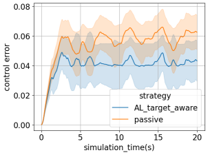
Figure 1: Results on pendulum simulator for a specific target. Left: The test loss of the estimated model $\hat{f}$. The passive strategy suffers from negative transfer while the active strategy steadily decreases. Right: The control error using final output $\hat{f}$. Here we use a model-based nonlinear policy $\pi(x,\hat{f})$. The model learned from active strategy leads to better control performance.

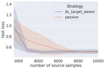
Figure 2: Results on the real drone dataset [7] with target drone_type_A_30_z. Source data includes two drone types A and B, six wind speeds from 0 to 50, and three directions x-y-z. We present results for linear $\phi_{X}$ here and postpone the non-linear $\phi_{X}$ case in Appendix D.3. Left: The test loss of the estimated bilinear model $\hat{f}$. The passive strategy converges slower than the active strategy. Right: Top 10 the most similar source tasks. Given the target environment, the algorithm successfully finds the other drone_type_A environments as relevant sources. See more explanations in Appendix D.3.

A typo in Theorem 4.1 in the main submission

We notice that there is a typo in the Theorem 4.1 in our submitted main paper, so we provide a correct version here. Therefore, you may find some terms in the main paper in this file are different from the one submitted before. We apologize for the inconvenience. We want to emphasize that this typo does not affect the main conclusion of our paper. It only affects the comparison between our upper bound and previous passive learning results in a specific setting.

Contents

1. 1 Introduction
   1. 1.1 Summery of contributions
2. 2 Preliminary
   1. 2.1 Goals
3. 3 A general framework
4. 4 A theoretical analysis under the benign ${\mathcal{W}}_{\text{source}}$ setting
   1. 4.1 Assumptions
   2. 4.2 Algorithm
   3. 4.3 Results
5. 5 Experiment
   1. 5.1 Settings
   2. 5.2 Results
6. A Result and analysis for target-aware
   1. A.1 Offline training oracles used in Algorithm
      1. A.1.1 Choice of ${\mathcal{O}}_{\text{offline 1}}^{X}$
      2. A.1.2 Choice of ${\mathcal{O}}_{\text{offline 2}}^{X}$
      3. A.1.3 Choice of ${\mathcal{O}}_{\text{offline}}^{W}$
   2. A.2 Excess risk analysis
      1. A.2.1 Reduce to an optimal design problem
      2. A.2.2 Bound decomposition and the excess risk result
      3. A.2.3 Detail proofs for warm-up stage
      4. A.2.4 Detail proofs for task-agnostic exploration strategy
      5. A.2.5 Auxillary lemmas
   3. A.3 Lemmas about the properties of $W^{\prime}$
   4. A.4 Sample complexity analysis – Formal version of Theorem 4.1
   5. A.5 More interpretation on results
7. B Results and analysis for target-agnostic
   1. B.1 Algorithm for target-agnostic
   2. B.2 Results and analysis
   3. B.3 Compare to previous passive learning and the target-aware one
8. C Limitations from the theoretical perspective
9. D Experiment details
   1. D.1 Synthetic data
      1. D.1.1 Settings
      2. D.1.2 Results
   2. D.2 Pendulum simulator
      1. D.2.1 Settings
      2. D.2.2 Results
   3. D.3 Real-world drone flight dataset
      1. D.3.1 Settings
      2. D.3.2 Results

Appendix A Result and analysis for target-aware

A.1 Offline training oracles used in Algorithm

A.1.1 Choice of ${\mathcal{O}}_{\text{offline 1}}^{X}$

To better illustrate this oracle ${\mathcal{O}}_{\text{offline}}^{X}$, we first give the following definition.

Definition A.1 (Modified from Assumption 2 in [12]).

For any $t$ tasks with parameter matrix $\dot{V}=[\dot{v}_{1},\dot{v}_{2},\ldots,\dot{v}_{t}]\in\mathbb{R}^{d_{W}\times t}$. Let $\lambda_{1}^{*}$ and $\lambda_{k}^{*}$ denote the largest and smallest eigenvalues of the task diversity matrix $(k/t)B_{W}^{\text{source}}\dot{V}\dot{V}^{\top}(B_{W}^{\text{source}})^{\top}\in\mathbb{R}^{k\times k}$ respectively. Then we say $\dot{V}$ is $\mu$-incoherent, i.e.,

$$\max_{i\in[t]}\left\|B_{W}^{\text{source}}\dot{v}_{i}\right\|^{2}\leq\mu\lambda_{k}^{*}$$

Notice that here $\dot{V}$ is a general representation of collected source tasks used for training in the different stages. Therefore, the $\lambda_{k}^{*},\mu$ is also defined differently corresponding to each stage. Specially, we have

• Stage 1( data collected by $q_{0}$):

  • $t=d_{W},\dot{V}=I_{d_{W}}$

  • $\lambda_{k}^{*}=\frac{k}{d_{W}}\sigma_{k}^{2}(B_{W}^{\text{source}})$

  • $\mu\geq\frac{1}{\lambda_{k}^{*}}$

• Stage 2( data collected by $q_{1}$):

  • $t=k,\dot{V}=V$ where $\_,\_,V\leftarrow\text{SVD}(\hat{B}_{W}^{\text{source}})$ as defined in line 5

  • $\lambda_{k}^{*}=\sigma_{k}^{2}(B_{W}^{\text{source}})$

  • $\mu\geq\frac{\sigma_{\text{max}}^{2}(B_{W}^{\text{source}})}{\lambda_{k}^{*}}$

Note that $\lambda_{k}^{*}=\sigma_{k}^{2}(B_{W}^{\text{source}})$ in the stage 2 comes from $B_{W}^{\text{source}}\dot{V}\dot{V}^{\top}(B_{W}^{\text{source}})^{\top}=\Theta(B_{W}^{\text{source}}(B_{W}^{\text{source}})^{\top})$ which will be proved later. Therefore, applying these results to

Now we restate the generalization guarantees from a fixed design (passive learning)

Theorem A.1 (Restate Theorem 1 in [12]).

Let there be $t$ linear regression tasks, each with $m$ samples, and

$$m\geq\widetilde{\Omega}\left(\left(1+k\left(\sigma/\sqrt{\lambda_{k}^{*}}\right)^{2}\right)k\log t+k^{2}\right),\quad\text{ and }mt\geq\widetilde{\Omega}\left(\left(1+\left(\sigma/\sqrt{\lambda_{k}^{*}}\right)^{2}\right)\left(\lambda_{1}^{*}/\lambda_{k}^{*}\right)\mu d_{X}k^{2}\right)$$

Then MLLAM, initialized at $\hat{B}_{X}=U_{\mathrm{init}}$ s.t. $\left\|\left(\mathbf{I}-B_{X}\left(B_{X}\right)^{\top}\right)U_{\mathrm{init}}\right\|_{F}\leq\min\left(3/4,O\left(\sqrt{\lambda_{k}^{*}/\lambda_{1}^{*}}\right)\right)$ and run for $K=\left\lceil\log_{2}\left(\lambda_{k}^{*}\lambda_{k}^{*}mt/\lambda_{1}^{*}\sigma^{2}\mu d_{X}k^{2}\right)\right\rceil$ iterations, outputs $\hat{B}_{X}$ so that the following holds $\left(w.p\right.$. $\left.\geq 1-K/(d_{X}k)^{10}\right)$

$$\sin(\hat{B}_{X},B_{X})\leq\left\|\left(\mathbf{I}-B_{X}\left(B_{X}\right)^{\top}\right)\hat{B}_{X}\right\|_{F}\leq\widetilde{O}\left(\left(\frac{\sigma}{\sqrt{\lambda_{k}^{*}}}\right)k\sqrt{\frac{\mu d_{X}}{mt}}\right)$$

Specifically, suppose we satisfy all the requirements in the theorem and run the proper amount of times, then we can guarantee $\hat{B}_{X}$ after each stage $j$ with w.h.p $\geq 1-2K/(d_{X}k)^{10}$

• Stage 1( data collected by $q_{0}$): $\sin(\hat{B}_{X},B_{X})\leq\widetilde{\mathcal{O}}\left(\sigma k\sqrt{\frac{d_{X}}{n_{0}}}\right)$

• Stage 2( data collected by $q_{1}$): $\sin(\hat{B}_{X},B_{X})\leq\widetilde{\mathcal{O}}\left(\sigma k\sqrt{\frac{d_{X}\sigma_{\text{max}}^{2}(B_{W}^{\text{source}})}{n_{0}}}\right)$

Let Event ${\mathcal{E}}_{\text{offline 1}}$ denote the above guarantees hold for all epochs.

A.1.2 Choice of ${\mathcal{O}}_{\text{offline 2}}^{X}$

We use the ERM from [9]. For readers’ convenience, we restate the formal definition of oracle below

$$\hat{B}_{X}=\operatorname*{arg\,min}_{B}\sum_{w|q_{1}(w)\neq 0\text{ and }q_{2}(w)\neq 0}\operatorname*{arg\,min}_{w}\sum_{(x,y)\in Z_{w}}\|x^{\top}w-y\|_{2}$$

By using this ERM with the follow-up finetune on $Z_{\text{target}}$, we get the following claims. Note that this claim comes from some part of Proof of Theorem 4.1 in the previous paper and has also been used in Claim 3 in [8].

Claim A.1.

By running the ERM-based algorithm, we get the following upper bounds,

$$\textsc{ER}(\tilde{B}_{X},\nu_{\text{target}}) \leq\mathbb{E}_{w_{0}\sim\nu_{\text{target}}}\left[\frac{\|P_{X_{\text{target}}\hat{B}_{X}}^{\bot}X_{\text{target}}B_{X}B_{W}w_{0}\|^{2}}{n_{\text{target}}}+\sigma^{2}\frac{k+\log(1/\delta)}{n_{\text{target}}}\right]$$

We need to admit that, from a theoretical perspective, we choose this oracle since we can directly use their conclusions. But other oracles like ${\mathcal{O}}_{\text{offline 2}}^{X}$ might also work.

A.1.3 Choice of ${\mathcal{O}}_{\text{offline}}^{W}$

This is the ERM oracle based on learned $\hat{B}_{X}$. Specially, we have $\hat{B}_{W}^{\text{source/target}}\leftarrow{\mathcal{O}}_{\text{offline}}^{W}(\{Z_{w}\}_{w|q(w)\neq 0},\hat{B}_{X})$ defined as

$$\hat{B}_{W}^{\text{source/target}}=\sum_{w|q(w)\neq 0}\hat{w}_{w}w^{\top},\text{ where }\hat{w}_{w}=\operatorname*{arg\,min}_{\hat{w}\in\mathbb{R}^{k}}\sum_{(x,y)\sim Z_{w}}\|x^{\top}\hat{B}_{X}^{\top}\hat{w}-y\|_{2},$$

A.2 Excess risk analysis

Theorem A.2 (Excess risk guarantees).

By running the Algo. 2, after epoch $j$, as long as ${\mathcal{E}}_{\text{offline 1}}$ holds, we have w.h.p $1-\delta$,

$$\textsc{ER}(\tilde{B}_{X},\nu_{\text{target}})\leq\widetilde{\mathcal{O}}\left(\sigma^{2}kd_{X}k^{*}\epsilon_{j}^{2}\right)$$

as long as

$$\dot{n}_{\text{target}}\geq\epsilon_{j}^{-\frac{4}{3}}d_{X}^{-\frac{2}{3}}\left(k^{-\frac{2}{3}}d_{W}^{\frac{1}{2}}\underline{\sigma}^{-\frac{4}{3}}+k^{-\frac{4}{3}}d_{W}^{\frac{1}{6}}\bar{\kappa}^{2}\underline{\sigma}^{-\frac{1}{3}}\right)\sqrt{k+\log(d_{W}/\delta)}$$

$$n_{\text{target}}\geq\epsilon_{j}^{-2}d_{X}^{-1}(k^{*})^{-1}\frac{k}{k+\log(d_{W}/\delta)}$$

Proof.

Here we provide the proof sketches, which will be specified in the following sections.

In Section A.2.1, we first reduce $\textsc{ER}(\tilde{B}_{X},\nu_{\text{target}})$ to an optimal design problem by showing that, with a proper number of $n_{\text{target}}$,

$$\textsc{ER}(\tilde{B}_{X},\nu_{\text{target}})\lessapprox(kd_{X}+\log(1/\delta))\text{Tr}\left(\left((B_{W}^{\text{source}})\left(\sum_{w\in{\mathcal{S}}}n_{w}ww^{\top}\right)(B_{W}^{\text{source}})^{\top}\right)^{-1}B_{W}\left(\mathbb{E}_{\nu_{\text{target}}}ww^{T}\right)B_{W}^{\top}\right)$$

It is easy to see that, as long as $B_{W}$ is known. The problem is reduced to an optimal design problem with fixed optimization target.

So the main challenge here is to iteratively estimate $B_{X},B_{W}$ and design the budget allocation to different sources. Therefore, in Section A.2.2, we further decompose the it into

$$\text{Tr}\left(\left((B_{W}^{\text{source}})\left(\sum_{w\in{\mathcal{S}}}n_{w}ww^{\top}\right)(B_{W}^{\text{source}})^{\top}\right)^{-1}B_{W}\left(\mathbb{E}_{\nu_{\text{target}}}ww^{T}\right)B_{W}^{\top}\right)$$

$$\leq\underbrace{\mathbb{E}_{w_{0}\sim\nu_{\text{target}}}(\left[(B_{W}w_{0})^{\top}\square B_{W}w_{0}\right]-\text{Tr}\left(\beta_{3}(B_{W}W^{\prime})^{\top}\square B_{W}W^{\prime}\right)}_{\text{target agnostic exploration error}}+\beta_{3}\underbrace{\text{Tr}\left((B_{W}W^{\prime})^{\top}\square B_{W}W^{\prime}\right)}_{\text{target-aware exploration error}}$$

where $\square=\left(B_{W}\left(\sum_{w\in{\mathcal{S}}}n_{w}ww^{\top}\right)B_{W}^{\top}\right)^{-1}$. Here the target-aware exploration error captures the error from selecting the target-related sources (defined by $q_{2}$). On the other hand, the target agnostic exploration error captures the error from model estimation and the uniform exploration.

Now the main challenge here is to upper-bound the model estimation error. Specifically, the estimation comes from Coarse exploration (Stage 1) and Fine target-agnostic exploration (Stage 2). Specifically, in Section A.2.3, we show that the $k$-dim-subspace represented by $q_{1}$ is a good course approximation up to multiplicative error. Then in Section A.2.4, we further tight the upper bound using data collected according to up to some additive error. ∎

A.2.1 Reduce to an optimal design problem

For any fixed epoch $j$, let $n_{w}^{j}$ denotes the samples collected so far for task $w$ and ${\mathcal{S}}$ denotes the set of tasks used in computing $\tilde{B}_{X}$. Therefore, we have ${\mathcal{S}}=\{w|q_{1}(w)\neq 0\text{ and }\tilde{q}(w)\neq 0\}$ and $n_{w}\geq n_{2}(w)+n_{2}^{j}(w)$. For convenience, we omit the superscript $j$ in the rest of the proofs.

From Claim A.1, it is easy to see that our main target is to optimize $\mathbb{E}_{w_{0}\sim\nu_{\text{target}}}\|P_{X_{\text{target}}\hat{B}_{X}}^{\bot}X_{\text{target}}B_{X}B_{W}w_{0}\|^{2}$. Decompose $B_{W}\left(\sum_{w\in{\mathcal{S}}}n_{w}ww^{\top}\right)B_{W}^{\top}$ as $UDU^{\top}$ and let $\Sigma_{W}=U\sqrt{D}U^{\top}$. As long as $\Sigma_{W}$ is full rank, which we will prove later in Section A.2.3, we have with probability $1-\delta$,

$$\mathbb{E}_{w_{0}\sim\nu_{\text{target}}}\|P_{X_{\text{target}}\hat{B}_{X}}^{\bot}X_{\text{target}}B_{X}B_{W}w_{0}\|^{2}$$

$$=\mathbb{E}_{w_{0}\sim\nu_{\text{target}}}\|P_{X_{\text{target}}\hat{B}_{X}}^{\bot}X_{\text{target}}B_{X}\Sigma_{W}^{\frac{1}{2}}\Sigma_{W}^{-\frac{1}{2}}B_{W}w_{0}\|^{2}$$

$$\leq\mathbb{E}_{w_{0}\sim\nu_{\text{target}}}\|P_{X_{\text{target}}\hat{B}_{X}}^{\bot}X_{\text{target}}B_{X}\Sigma_{W}^{\frac{1}{2}}\|_{F}^{2}\|\Sigma_{W}^{-\frac{1}{2}}B_{W}w_{0}\|^{2}$$

$$=\mathbb{E}_{w_{0}\sim\nu_{\text{target}}}\|P_{X_{\text{target}}\hat{B}_{X}}^{\bot}X_{\text{target}}B_{X}B_{W}\tilde{W}_{\mathcal{S}}\|_{F}^{2}(B_{W}w_{0})^{\top}\left(B_{W}\left(\sum_{w\in{\mathcal{S}}}n_{w}ww^{\top}\right)B_{W}^{\top}\right)^{-1}B_{W}w_{0}$$

$$=\|P_{X_{\text{target}}\hat{B}_{X}}^{\bot}X_{\text{target}}B_{X}B_{W}\tilde{W}_{\mathcal{S}}\|_{F}^{2}\text{Tr}\left(\left(B_{W}\left(\sum_{w\in{\mathcal{S}}}n_{w}ww^{\top}\right)B_{W}^{\top}\right)^{-1}B_{W}\left(\mathbb{E}_{\nu_{\text{target}}\in\Delta({\mathcal{W}}_{\text{target}})}ww^{T}\right)B_{W}^{\top}\right)$$

$$\lessapprox\sigma^{2}n_{\text{target}}\left(kd_{X}+\log(1/\delta)\right)\text{Tr}\left(\left(B_{W}\left(\sum_{w\in{\mathcal{S}}}n_{w}ww^{\top}\right)B_{W}^{\top}\right)^{-1}B_{W}\left(\mathbb{E}_{\nu_{\text{target}}}ww^{T}\right)B_{W}^{\top}\right)$$

$$=\sigma^{2}n_{\text{target}}\left(kd_{X}+\log(1/\delta)\right)\text{Tr}\left(\left((B_{W}^{\text{source}})\left(\sum_{w\in{\mathcal{S}}}n_{w}ww^{\top}\right)(B_{W}^{\text{source}})^{\top}\right)^{-1}B_{W}\left(\mathbb{E}_{\nu_{\text{target}}}ww^{T}\right)B_{W}^{\top}\right)$$

Therefore, we aim to minimize the $\text{Tr}\left(\left((B_{W}^{\text{source}})\left(\sum_{w\in{\mathcal{S}}}n_{w}ww^{\top}\right)(B_{W}^{\text{source}})^{\top}\right)^{-1}B_{W}\left(\mathbb{E}_{\nu_{\text{target}}}ww^{T}\right)B_{W}^{\top}\right)$. As we mentioned before, this is a pure optimal design problem if $B_{W}$ is known in advance.

A.2.2 Bound decomposition and the excess risk result

Let $\square=\left(B_{W}\left(\sum_{w\in{\mathcal{S}}}n_{w}ww^{\top}\right)B_{W}^{\top}\right)^{-1}$, we have

$$\mathbb{E}_{w_{0}\sim\nu_{\text{target}}}\left[(B_{W}w_{0})^{\top}\square B_{W}w_{0}\right]$$

$$=\underbrace{\mathbb{E}_{w_{0}\sim\nu_{\text{target}}}(\left[(B_{W}w_{0})^{\top}\square B_{W}w_{0}\right]-\text{Tr}\left(\beta_{3}(B_{W}W^{\prime})^{\top}\square B_{W}W^{\prime}\right)}_{\text{target agnostic exploration error}}+\beta_{3}\underbrace{\text{Tr}\left((B_{W}W^{\prime})^{\top}\square B_{W}W^{\prime}\right)}_{\text{target-aware exploration error}}$$

We first deal with the target-aware exploration error. It is easy to see that

$$\beta_{3}\text{Tr}\left((B_{W}W^{\prime})^{\top}\square B_{W}W^{\prime}\right)$$

$$=\beta_{3}\text{Tr}\left(\left(B_{W}\sum_{w}q_{1}(w)n_{1}ww^{\top}(B_{W})^{\top}+B_{W}\sum_{w}q_{2}(w)n_{2}ww^{\top}(B_{W})^{\top}\right)^{-1}B_{W}W^{\prime}(B_{W}W^{\prime})^{\top}\right)$$

$$\leq\text{Tr}\left(\left(\max_{i}\|\tilde{W}(i)\|_{2(\infty)}^{2}B_{W}\epsilon^{-2}\tilde{W}\tilde{W}^{\top}(B_{W})^{\top}\right)^{-1}B_{W}W^{\prime}(B_{W}W^{\prime})^{\top}\right)$$

$$\leq\text{Tr}\left(\left(B_{W}\epsilon^{-2}W^{\prime}(W^{\prime})^{\top}(B_{W})^{\top}\right)^{-1}B_{W}W^{\prime}(B_{W}W^{\prime})^{\top}\right)$$

$$=\epsilon^{2}\text{rank}(\hat{B}_{W}W^{\prime}(W^{\prime})^{\top}\hat{B}_{W}^{\top})$$

$$\leq\epsilon^{2}\text{rank}(B_{W}\mathbb{E}_{\nu_{\text{target}}}[w_{0}w_{0}^{\top}]B_{W}^{\top})$$

where the last equality comes from Lemma A.5.

We then deal with the target-agnostic exploration term. Let the clipping threshold in Line 9 be $\bar{\gamma}_{j}$. That is, ignoring all $\lambda_{i}\leq\bar{\gamma}$. Now, for $\beta_{3}\geq 8$, when event ${\mathcal{E}}_{\text{offline 1}}$, holds, we have w.h.p $1-d_{W}\delta$

$$\mathbb{E}_{w_{0}\sim\nu_{0}}\left[(B_{W}w_{0})^{\top}\square B_{W}w_{0}\right]-\beta_{3}\text{Tr}\left((B_{W}W^{\prime})^{\top}\square B_{W}W^{\prime}\right)$$

$$=\mathbb{E}_{w_{0}\sim\nu_{0}}\text{Tr}\left(\square\left(B_{W}w_{0}(B_{W}w_{0})^{\top}-4\hat{B}_{W}^{\text{target}}w_{0}(\hat{B}_{W}^{\text{target}}w_{0})^{\top}\right)\right)$$

$$\quad+\mathbb{E}_{w_{0}\sim\nu_{0}}\text{Tr}\left(\square\left(\frac{1}{2}\beta_{3}\hat{B}_{W}^{\text{source}}w^{\prime}(\hat{B}_{W}w^{\prime})^{\top}-\beta_{3}B_{W}^{\text{source}}w^{\prime}(B_{W}w^{\prime})^{\top}\right)\right)$$

$$\quad+\mathbb{E}_{w_{0}\sim\nu_{0}}\text{Tr}\left(\square\left(4\hat{B}_{W}^{\text{target}}w_{0}(\hat{B}_{W}^{\text{target}}w_{0})^{\top}-\frac{1}{2}\beta_{3}\hat{B}_{W}^{\text{source}}W^{\prime}(\hat{B}_{W}^{\text{source}}W^{\prime})^{\top}\right)\right)$$

$$\leq\mathbb{E}_{w_{0}\sim\nu_{0}}\text{Tr}\left(\left(4B_{W}^{\text{target}}w_{0}(B_{W}^{\text{target}}w_{0})^{\top}-4\hat{B}_{W}^{\text{target}}w_{0}(\hat{B}_{W}^{\text{target}}w_{0})^{\top}\right)\right)\|\square\|$$

$$\quad+\beta_{3}\text{Tr}\left(\left(\frac{1}{2}\hat{B}_{W}^{\text{source}}w^{\prime}(\hat{B}_{W}w^{\prime})^{\top}-\frac{1}{2}\dot{B}_{W}W^{\prime}(\dot{B}_{W}W^{\prime})^{\top}\right)\right)\|\square\|$$

$$\quad+k\overline{\gamma}\|\square\|$$

$$\leq\|\square\|\|\mathbb{E}[w_{0}w_{0}^{T}]\|_{*}\|(B_{W}^{\text{target}})^{\top}B_{W}^{\text{target}}-(\hat{B}_{W}^{\text{target}})^{\top}\hat{B}_{W}^{\text{target}}\|+\|\square\|\|W^{\prime}(W^{\prime})^{\top}\|_{*}\|\dot{B}_{W}^{\top}\dot{B}_{W}-\hat{B}_{W}^{\top}\hat{B}_{W}\|+k\overline{\gamma}\|\square\|$$

$$\leq 2\|\square\|\|\mathbb{E}[w_{0}w_{0}^{T}]\|_{*}\|B_{W}^{\text{target}}-\hat{B}_{W}^{\text{target}}\|\|B_{W}^{\text{target}}\|$$

$$\quad+2\|\square\|\|\|W^{\prime}(W^{\prime})^{\top}\|_{*}\|\dot{B}_{W}-\hat{B}_{W}^{\text{source}}\|\|\hat{B}_{W}^{\text{source}}\|$$

$$\quad+k\overline{\gamma}\|\square\|$$

$$\leq\epsilon^{2}$$

where the second two terms in the first inequality come from Section A.2.3 and the last term in the first inequality comes from the definition of $W^{\prime}$. Here $\dot{B}_{W}=B_{W}VV^{\top}=B_{W}^{\text{source}}VV^{\top}$ is a pseudo representation of $B_{W}^{\text{source}}$, where $V$ is the one calculated in Line 5. And the last inequality comes from the results in Section A.2.4. Notice that the probability $1-d_{W}\delta$ comes from the union bound on all the calls of ${\mathcal{O}}_{\text{offline}}^{W}$.

Now combine the bounds above, we have

$$\textsc{ER}(\tilde{B}_{X},\nu_{\text{target}}) \leq\sigma^{2}\left(kd_{X}\log((\kappa N_{i})/d_{W})+\log\frac{1}{\delta}\right)k^{*}\epsilon^{2}$$

A.2.3 Detail proofs for warm-up stage

After the first stage, according to Section A.1.1, as long as ${\mathcal{E}}_{\text{offline 1}}$ holds, we have

$$\sin(\hat{B}_{X},B_{X})\leq\widetilde{\mathcal{O}}\left(\sigma k\sqrt{\frac{d_{X}}{n_{0}}}\right)$$

Therefore, by Lemma A.2, we have with probability $1-d_{W}\delta$,

$$\|\hat{B}_{W}^{\text{source}}-B_{W}^{\text{source}}\| \leq 2\sqrt{k}\sin(\hat{B}_{X},B_{X})\|B_{W}\|+\sqrt{\frac{d_{W}}{n_{0}}}(k+\log(2/\delta)^{\frac{1}{4}}d_{W}^{\frac{1}{4}}$$

$$\leq 2k^{\frac{3}{2}}\sqrt{\frac{d_{X}}{n_{0}}}\|B_{W}\|+2d_{W}^{\frac{3}{4}}(k+\log(2/\delta)^{\frac{1}{4}}\sqrt{\frac{1}{n_{0}}}$$

As long as $n_{0}\geq 1024\bar{\kappa}^{2}\left(k^{3}d_{X}\bar{\kappa}^{2}+\frac{d_{W}^{\frac{3}{2}}}{\underline{\sigma}^{2}}\sqrt{k+\log(1/\delta)}\right)$, by using the Lemma A.1 below, we have for any arbitrary matrix $M$,

$$\frac{1}{2}B_{W}M(B_{W})^{\top}\leq\dot{B}_{W}M\dot{B}_{W}^{\top}\leq\frac{3}{2}B_{W}M(B_{W})^{\top}$$

In the other word, $\dot{B}$ can be regarded as a pseudo representation of $B_{W}^{\text{source}}$. In all the later epochs, when exploring $k$-subspace according to $q_{1}^{j}$, the learner actually learns $\dot{B}_{W}$.

Lemma A.1 (Guarantee on exploration basis 1).

Suppose we have the estimated $\hat{B}_{W}$ satisfies

$$8\|B_{W}-\hat{B}_{W}\|\|B_{W}\|\leq\frac{1}{2}\lambda_{\min}(B_{W}B_{W}^{\top})$$

$$\dot{V}\leftarrow\text{column space of }\textsc{SVD}(\hat{B}_{W}),$$

then let $\dot{B}_{W}=B_{W}\dot{V}\dot{V}^{\top}$, we have, for any arbitrary matrix $M$,

$$\frac{1}{2}B_{W}M(B_{W})^{\top}\leq\dot{B}_{W}M\dot{B}_{W}^{\top}\leq\frac{3}{2}B_{W}M(B_{W})^{\top}$$

Proof.

$$\dot{B}_{W}M\dot{B}_{W}^{\top}-B_{W}M(B_{W})^{\top}$$

$$=\dot{B}_{W}M\dot{B}_{W}^{\top}-\hat{B}_{W}M(\hat{B}_{W})^{\top}+\hat{B}_{W}M(\hat{B}_{W})^{\top}-B_{W}MB_{W}^{\top}$$

$$=(\dot{B}_{W}-\hat{B}_{W})MB_{W}^{\top}+\hat{B}_{W}M(\dot{B}_{W}-\hat{B}_{W})^{\top}+(\hat{B}_{W}-B_{W})M(\hat{B}_{W})^{\top}+B_{W}M(\hat{B}_{W}-B_{W})^{\top}$$

$$=(B_{W}-\hat{B}_{W})\dot{V}\dot{V}^{\top}MB_{W}^{\top}+\hat{B}_{W}M\dot{V}\dot{V}^{\top}(B_{W}-\hat{B}_{W})^{\top}+(\hat{B}_{W}-B_{W})M(\hat{B}_{W})^{\top}+B_{W}M(\hat{B}_{W}-B_{W})^{\top}$$

Therefore, according to our assumption, we can upper bound the above as

$$\dot{B}_{W}M\dot{B}_{W}^{\top}-B_{W}M(B_{W})^{\top} \leq 2\|B_{W}-\hat{B}_{W}\|\left(\|\hat{B}_{W}\|+\|B_{W}\|\right)M$$

$$\leq\left(4\|B_{W}-\hat{B}_{W}\|\|B_{W}\|+2\|B_{W}-\hat{B}_{W}\|_{2}^{2}\right)M$$

$$\leq 8\|B_{W}-\hat{B}_{W}\|\|B_{W}\|M$$

$$\leq\frac{1}{2}\lambda_{\min}(B_{W}B_{W}^{\top})M\leq\frac{1}{2}B_{W}MB_{W}^{\top}$$

Similarly, it can be lower bounded by $-\frac{1}{2}B_{W}MB_{W}^{\top}$. Therefore we can get the target result by rearranging. ∎

A.2.4 Detail proofs for task-agnostic exploration strategy

First, we upper bound two $\|B_{W}-\hat{B}_{W}\|$ terms. From section A.1.1, as long as ${\mathcal{E}}_{\text{offline 1}}$ holds, we have

$$\sin(\hat{B}_{X},B_{X})\leq\widetilde{\mathcal{O}}\left(k\sqrt{\frac{d_{X}}{n_{1}}}\|B_{W}^{\text{source}}\|\right)$$

Therefore, by Lemma A.2, we have w.h.p at least $1-(k+d_{W}^{\text{target}})\delta$

$$\|\hat{B}^{\text{source}}_{W}-B_{W}^{\text{source}}\| \leq 2\sqrt{k}\sin(\hat{B}_{X},B_{X})\|B_{W}^{\text{source}}\|+\sqrt{\frac{k}{n_{1}}}(k+\log(2/\delta)^{\frac{1}{4}}k^{\frac{1}{4}}$$

$$\leq 2k^{\frac{3}{2}}\sqrt{\frac{d_{X}}{n_{1}}}\|B_{W}^{\text{source}}\|^{2}$$

$$\|\hat{B}^{\text{target}}_{W}-B_{W}^{\text{target}}\| \leq 2k\sin(\hat{B}_{X},B_{X})\|B_{W}^{\text{target}}\|+\sqrt{\frac{1}{\dot{n}_{\text{target}}}}(k+\log(2/\delta)^{\frac{1}{4}}(d_{W}^{\text{target}})^{\frac{1}{4}}$$

$$\leq 2k^{\frac{3}{2}}\sqrt{\frac{d_{X}}{n_{1}}}\|B_{W}^{\text{target}}\|^{2}+2\sqrt{\frac{1}{\dot{n}_{\text{target}}}}(k+\log(2/\delta)^{\frac{1}{4}}(d_{W}^{\text{target}})^{\frac{1}{4}}$$

$$\leq 4k^{\frac{3}{2}}\sqrt{\frac{d_{X}}{n_{1}}}\|B_{W}^{\text{target}}\|^{2}$$

where the last equality holds as long as $\dot{n}_{\text{target}}\geq n_{1}\frac{\sqrt{(k+\log(2/\delta))d_{W}^{\text{target}}}}{k^{3}d_{X}\|B_{W}^{\text{target}}\|^{2}}$.

Next, we upper bound the $\|W^{\prime}(W^{\prime})\|$ according to Lemma A.7.

$$\|W^{\prime}(W^{\prime})^{\top}\|_{*} \lessapprox\frac{1}{\sigma_{\min}^{2}(B_{W}^{\text{source}})}\|B_{W}^{\text{target}}\mathbb{E}_{\nu_{\text{target}}}[w_{0}w_{0}^{\top}](B_{W}^{\text{target}})^{\top}\|_{*}$$

$$\leq\frac{1}{\sigma_{\min}^{2}(B_{W}^{\text{source}})}\|B_{W}^{\text{target}}\|^{2}\|\mathbb{E}_{\nu_{\text{target}}}[w_{0}w_{0}^{\top}]\|_{*}$$

$$\leq\frac{1}{\sigma_{\min}^{2}(B_{W}^{\text{source}})}\|B_{W}^{\text{target}}\|^{2}$$

Finally, we have, by definition

$$\bar{\gamma}\leq 2\|\hat{B}_{W}^{\text{target}}-B_{W}^{\text{target}}\|\|B_{W}^{\text{target}}\|$$

$$\|\square\|\leq\frac{k}{n_{1}\sigma_{\min}^{2}(\dot{B}_{W})}\lessapprox\frac{k}{n_{1}\sigma_{\min}^{2}(B_{W}^{\text{source}})}$$

Combine all above, we have the upper bound

$$\|\square\|\left(\|\mathbb{E}[w_{0}w_{0}^{T}]\|_{*}\|B_{W}^{\text{target}}-\hat{B}_{W}^{\text{target}}\|\|B_{W}^{\text{target}}\|+\|\|W^{\prime}(W^{\prime})^{\top}\|_{*}\|\dot{B}_{W}-\hat{B}_{W}^{\text{source}}\|\|B_{W}^{\text{source}}\|+k\overline{\gamma}\right)$$

$$\lessapprox\frac{k}{n_{1}\sigma_{\min}^{2}(B_{W}^{\text{source}})}*k^{\frac{3}{2}}\sqrt{\frac{d_{X}}{n_{1}}}*\left(k\|B_{W}^{\text{target}}\|^{3}+\|B_{W}^{\text{source}}\|\|B_{W}^{\text{target}}\|^{2}\bar{\kappa}^{2}\right)$$

$$\leq k^{\frac{5}{2}}d_{X}^{\frac{1}{2}}n_{1}^{-\frac{3}{2}}\|B_{W}^{\text{target}}\|^{2}\left(\frac{k\|B_{W}^{\text{target}}\|}{\underline{\sigma^{2}}}+\frac{\bar{\kappa}^{3}}{\underline{\sigma}}\right)$$

$$\leq k^{\frac{5}{2}}d_{X}^{\frac{1}{2}}n_{1}^{-\frac{3}{2}}d_{W}\left(k\sqrt{d_{W}}\underline{\sigma}^{-2}+\bar{\kappa}^{3}\underline{\sigma}^{-1}\right)$$

As long as $n_{1}\geq\epsilon_{j}^{-\frac{4}{3}}k^{\frac{5}{3}}d_{W}^{\frac{2}{3}}d_{X}^{\frac{1}{3}}\left(k^{\frac{2}{3}}d_{W}^{\frac{1}{3}}\underline{\sigma}^{-\frac{4}{3}}+\bar{\kappa}^{2}\underline{\sigma}^{-\frac{2}{3}}\right)$, we have the final bound $\epsilon_{j}^{2}$.

A.2.5 Auxillary lemmas

Lemma A.2.

Consider any $t$ regression tasks parameterized by $\{\dot{v}_{i}\}_{i\in[n]}$. Denote $\dot{V}=[\dot{v}_{1},\dot{v}_{2},\ldots,\dot{v}_{t}]$ and $|X_{\dot{v}_{i}}|=n$ for all $i\in[t]$, define

$$\hat{B}_{W}=\sum_{i\in k}\hat{w}_{i}\dot{v}_{i}^{\top},\text{ where }\hat{w}_{i}=\operatorname*{arg\,min}_{w\in\mathbb{R}^{k}}\|X_{\dot{v}_{i}}\hat{B}_{X}^{\top}w-Y_{\dot{v}_{i}}\|_{2},$$

then we have with probability at least $1-\delta$,

$$\|\hat{B}_{W}-\dot{B}_{W}\|=\|\hat{B}_{W}-B_{W}\dot{V}\dot{V}^{\top}\|\leq 2\sqrt{k}\sin(\hat{B}_{X},B_{X})\|\dot{B}_{W}\|+\sqrt{\frac{1}{n}}(k+\log(2/\delta)^{\frac{1}{4}}|\dot{V}|^{\frac{1}{4}}$$

Proof.

From [8], we get that the explicit form of $\hat{w}_{i}$, which is the estimation of actual $B_{w}\dot{v}_{i}$ as

$$\left(\hat{B}_{X}X_{\dot{v}_{i}}^{\top}X_{\dot{v}_{i}}\hat{B}_{X}^{\top}\right)^{-1}\hat{B}_{X}X_{\dot{v}_{i}}^{\top}X_{\dot{v}_{i}}B_{X}^{\top}B_{X}\dot{v}_{i}+\left(\hat{B}_{X}X_{\dot{v}_{i}}^{\top}X_{\dot{v}_{i}}\hat{B}_{X}^{\top}\right)^{-1}\hat{B}_{X}X_{\dot{v}_{i}}^{\top}\xi_{w}$$

By abusing notation a little bit, here we use subscription $i$ to denote the items that associate the task encoded by $\dot{v}_{i}$. Therefore, we have

$$\hat{B}_{W} =\sum_{i=1}^{t}\left(\hat{B}_{X}X_{i}^{\top}X_{i}\hat{B}_{X}^{\top}\right)^{-1}\hat{B}_{X}X_{i}^{\top}X_{i}B_{X}^{\top}B_{W}\dot{v}_{i}\dot{v}_{i}^{\top}+\sum_{i=1}^{t}\left(\hat{B}_{X}X_{i}^{\top}X_{i}\hat{B}_{X}^{\top}\right)^{-1}\hat{B}_{X}X_{i}^{\top}\mathbf{\xi}_{i}\dot{v}_{i}^{\top}$$

$$=\sum_{i=1}^{t}\left(\hat{B}_{X}X_{i}^{\top}X_{i}\hat{B}_{X}^{\top}\right)^{-1}\hat{B}_{X}X_{i}^{\top}X_{i}\left(\hat{B}_{X}^{\top}\hat{B}_{X}+\hat{B}_{X,\perp}^{\top}\hat{B}_{X,\perp}\right)B_{X}^{\top}B_{W}\dot{v}_{i}\dot{v}_{i}^{\top}$$

$$\quad+\sum_{i=1}^{t}\left(\hat{B}_{X}X_{i}^{\top}X_{i}\hat{B}_{X}^{\top}\right)^{-1}\hat{B}_{X}X_{i}^{\top}\mathbf{\xi}_{i}\dot{v}_{i}^{\top}$$

$$=\hat{B}_{X}B_{X}^{\top}\dot{B}_{W}+\sum_{i=1}^{t}\left(\hat{B}_{X}X_{i}^{\top}X_{i}\hat{B}_{X}^{\top}\right)^{-1}\hat{B}_{X}X_{i}^{\top}X_{i}\hat{B}_{X,\perp}^{\top}\hat{B}_{X,\perp}B_{X}^{\top}B_{W}\dot{v}_{i}\dot{v}_{i}^{\top}$$

$$\quad+\sum_{i=1}^{d}\left(\hat{B}_{X}X_{i}^{\top}X_{i}\hat{B}_{X}^{\top}\right)^{-1}\hat{B}_{X}X_{i}^{\top}\mathbf{\xi}_{i}\dot{v}_{i}^{\top}$$

And the estimation difference between $B_{W},\hat{B}_{W}$ can be decomposed into three parts

$$\|\dot{B}_{W}-\hat{B}_{W}\| \leq\|\left(\hat{B}_{X}B_{X}^{\top}-I_{k}\right)\dot{B}_{W}\|$$

$$\quad+\|\sum_{i=1}^{t}\left(\hat{B}_{X}X_{i}^{\top}X_{i}\hat{B}_{X}^{\top}\right)^{-1}\hat{B}_{X}X_{i}^{\top}X_{i}\hat{B}_{X,\perp}^{\top}\hat{B}_{X,\perp}B_{X}^{\top}B_{W}\dot{v}_{i}\dot{v}_{i}^{\top}\|$$

$$\quad+\|\sum_{i=1}^{t}\left(\hat{B}_{X}X_{i}^{\top}X_{i}\hat{B}_{X}^{\top}\right)^{-1}\hat{B}_{X}X_{i}^{\top}\mathbf{\xi}_{i}\dot{v}_{i}^{\top}\|$$

$$\leq\|\left(\hat{B}_{X}B_{X}^{\top}-I_{k}\right)\|\|\dot{B}_{W}\|$$

$$\quad+\max_{i}\|\left(\hat{B}_{X}X_{i}^{\top}X_{i}\hat{B}_{X}^{\top}\right)^{-1}\hat{B}_{X}X_{i}^{\top}X_{i}\hat{B}_{X,\perp}^{\top}\hat{B}_{X,\perp}B_{X}^{\top}\|\|\sum_{i=1}^{t}B_{W}\dot{v}_{i}\dot{v}_{i}^{\top}\|$$

$$\quad+\|\sum_{i=1}^{t}\left(\hat{B}_{X}X_{i}^{\top}X_{i}\hat{B}_{X}^{\top}\right)^{-1}\hat{B}_{X}X_{i}^{\top}\mathbf{\xi}_{i}\dot{v}_{i}^{\top}\|$$

By using Lemma A.3 and Lemma A.4, we can bound the first two terms by

$$2\sqrt{k}\sin(\hat{B}_{X},B_{X})\|\dot{B}_{W}\|$$

Now we are going to bound the last term which is the noise term.

$$\|\sum_{i=1}^{|\dot{V}|}\left(\hat{B}_{X}X_{i}^{\top}X_{i}\hat{B}_{X}^{\top}\right)^{-1}\hat{B}_{X}X_{i}^{\top}\mathbf{\xi}_{i}\dot{v}_{i}^{\top}\|^{2}$$

$$=\lambda_{\max}\left(\sum_{i=1}^{|\dot{V}|}\left(\hat{B}_{X}X_{i}^{\top}X_{i}\hat{B}_{X}^{\top}\right)^{-1}\hat{B}_{X}X_{i}^{\top}\mathbf{\xi}_{i}\dot{v}_{i}^{\top}\right)\left(\sum_{i=1}^{|\dot{V}|}\left(\hat{B}_{X}X_{i}^{\top}X_{i}\hat{B}_{X}^{\top}\right)^{-1}\hat{B}_{X}X_{i}^{\top}\mathbf{\xi}_{i}\dot{v}_{i}^{\top}\right)^{\top}$$

$$\leq\lambda_{\max}\left(\sum_{i=1}^{|\dot{V}|}\left(\hat{B}_{X}X_{i}^{\top}X_{i}\hat{B}_{X}^{\top}\right)^{-1}\hat{B}_{X}X_{i}^{\top}\xi_{i}\xi_{i}^{\top}X_{i}\hat{B}_{X}^{\top}\left(\hat{B}_{X}X_{i}^{\top}X_{i}\hat{B}_{X}^{\top}\right)^{-1}\right)$$

Note that, $x_{i}\sim{\mathcal{N}}(0,I_{d})$ and

$$\left(\hat{B}_{X}X_{i}^{\top}X_{i}\hat{B}_{X}^{\top}\right)^{-1}\hat{B}_{X}X_{i}^{\top}\xi_{i} \sim{\mathcal{N}}\left(0,\left(\left(\hat{B}_{X}X_{i}^{\top}X_{i}\hat{B}_{X}^{\top}\right)^{-1}\hat{B}_{X}X_{i}^{\top}X_{i}\hat{B}_{X}^{\top}\left(\hat{B}_{X}X_{i}^{\top}X_{i}\hat{B}_{X}^{\top}\right)^{-1}\right)\right)$$

$$\sim{\mathcal{N}}\left(0,\left(\hat{B}_{X}X_{i}^{\top}X_{i}\hat{B}_{X}^{\top}\right)^{-1}\right)$$

Therefore, by the concentration inequality of the covariance matrix, we have, w.h.p $1-\delta$,

$$\lambda_{\max}\left(\sum_{i=1}^{|\dot{V}|}\left(\hat{B}_{X}X_{i}^{\top}X_{i}\hat{B}_{X}^{\top}\right)^{-1}\hat{B}_{X}X_{i}^{\top}\xi_{i}\xi_{i}^{\top}X_{i}\hat{B}_{X}^{\top}\left(\hat{B}_{X}X_{i}^{\top}X_{i}\hat{B}_{X}^{\top}\right)^{-1}\right)\leq\frac{1}{n}\sqrt{(k+\log(2/\delta)|\dot{V}|}$$

Combining everything above, we have the final bound. ∎

Lemma A.3.

Given $\hat{B}_{X},B_{X}$ are orthonormal matrices, as well as $\mathbb{E}[xx^{T}]=I_{d_{X}}$ for all tasks $w$, we have

$$\|I_{k}-\hat{B}_{X}B_{X}^{\top}\|\leq\mathcal{O}\left(\sqrt{k}\sin(\hat{B}_{X},\hat{B}_{X})\right)$$

Proof.

Denote $B_{X}\hat{B}_{X}^{\top}=UDV^{\top}$, by definition, we have $D=\text{diag}(\cos{\theta_{1}},\cos{\theta_{2}},\ldots,\cos{\theta_{k}})$ from the largest singular value to minimum singular value and $\sin{\theta_{k}}\leq\sin(\hat{B}_{X},\hat{B}_{X})$. Therefore we have,

$$\text{Tr}(\hat{B}_{X}B_{X}^{\top})\geq k\sqrt{1-\sin^{2}(\hat{B}_{X},B_{X})}\geq k-k\sin^{2}(\hat{B}_{X},B_{X})$$

And

$$\|I_{k}-\hat{B}_{X}B_{X}^{\top}\|^{2} =\lambda_{\max}\left(I_{k}-\hat{B}_{X}B_{X}^{\top}\right)^{\top}\left(I_{k}-\hat{B}_{X}B_{X}^{\top}\right)$$

$$\leq\text{Tr}\left(I_{k}-\hat{B}_{X}B_{X}^{\top}\right)^{\top}\left(I_{k}-\hat{B}_{X}B_{X}^{\top}\right)$$

$$\leq\text{Tr}\left(I_{k}+\left(\hat{B}_{X}B_{X}^{\top}\right)^{\top}\hat{B}_{X}B_{X}^{\top}-\left(\hat{B}_{X}B_{X}^{\top}\right)^{\top}-\hat{B}_{X}B_{X}^{\top}\right)$$

$$\leq 2k-2k+2k\sin^{2}(\hat{B}_{X},B_{X})\leq 2k\sin^{2}(\hat{B}_{X},B_{X})$$

∎

Lemma A.4 (Restate from [11]).

Given $\hat{B}_{X},B_{X}$ are orthonormal matrices, as well as $\mathbb{E}[xx^{T}]=I_{d_{X}}$ for any fixed task $w$, we have

$$\|\left(\hat{B}_{X}X_{w}^{\top}X_{w}\hat{B}_{X}^{\top}\right)^{-1}\hat{B}_{X}X_{w}^{\top}X_{w}\hat{B}_{X,\perp}^{\top}\hat{B}_{X,\perp}B_{X}^{\top}\|\leq\sin(\hat{B}_{X},\hat{B}_{X})$$

Proof.

Here we follow the same proof step as in [11]. (Bound on the second error term in Lemma 19)

$$\|\left(\hat{B}_{X}X_{w}^{\top}X_{w}\hat{B}_{X}^{\top}\right)^{-1}\hat{B}_{X}X_{w}^{\top}X_{w}\hat{B}_{X,\perp}^{\top}\hat{B}_{X,\perp}B_{X}^{\top}\|$$

$$\leq\|\left(\hat{B}_{X}X_{w}^{\top}X_{w}\hat{B}_{X}^{\top}\right)^{-1}\hat{B}_{X}X_{w}^{\top}X_{w}\hat{B}_{X,\perp}^{\top}\|\sin(\hat{B}_{X},\hat{B}_{X})$$

$$\leq\sin(\hat{B}_{X},\hat{B}_{X})$$

∎

A.3 Lemmas about the properties of $W^{\prime}$

Lemma A.5.

$$\text{rank}(\hat{B}_{W}WW^{\prime}\hat{B}_{W}^{\top})\leq\text{rank}(B_{W}\mathbb{E}_{\nu_{\text{target}}}[w_{0}w_{0}^{\top}]B_{W}^{\top})$$

Proof.

By using Welys inequality, we have for any eigenvalue $i\in[k]$,

$$|\lambda_{i}\left(\hat{B}_{W}^{\text{target}}\mathbb{E}[w_{0}w_{0}^{\top}](\hat{B}_{W}^{\text{target}})^{\top}\right)-\lambda_{i}\left(B_{W}^{\text{target}}\mathbb{E}[w_{0}w_{0}^{\top}](B_{W}^{\text{target}})^{\top}\right)|$$

$$\leq\|\hat{B}_{W}^{\text{target}}\mathbb{E}[w_{0}w_{0}^{\top}](\hat{B}_{W}^{\text{target}})^{\top}-B_{W}^{\text{target}}\mathbb{E}[w_{0}w_{0}^{\top}](B_{W}^{\text{target}})^{\top}\|$$

$$\leq\|\hat{B}_{W}^{\text{target}}(\hat{B}_{W}^{\text{target}})^{\top}-B_{W}^{\text{target}}(B_{W}^{\text{target}})^{\top}\|$$

$$\leq 2\|\hat{B}_{W}^{\text{target}}-B_{W}^{\text{target}}\|\|B_{W}^{\text{target}}\|$$

$$\leq\left(2k^{\frac{3}{2}}\sqrt{\frac{d_{X}}{n_{1}}}\|B_{W}^{\text{source}}\|^{2}+2\sqrt{\frac{k}{\dot{n}_{\text{target}}}}\right)\|B_{W}^{\text{target}}\|$$

where the last inequality comes from Lemma A.2 and the fact $\sin(\hat{B}_{X},B_{X})\leq\widetilde{\mathcal{O}}\left(k\sqrt{\frac{d_{X}}{n_{1}}}\|B_{W}^{\text{source}}\|\right)$. Therefore, for all the $i\geq k^{*}$,

$$\lambda_{i}\left(\hat{B}_{W}^{\text{target}}\mathbb{E}[w_{0}w_{0}^{\top}](\hat{B}_{W}^{\text{target}})^{\top}\right)\geq\left(2k\sqrt{\frac{d_{X}}{n_{1}}}\|B_{W}^{\text{source}}\|^{2}+2\sqrt{\frac{k}{\dot{n}_{\text{target}}}}\right)\|B_{W}^{\text{target}}\|$$

Clipping those non-significant directions leads to the result. ∎

Lemma A.6.

Define $W_{i}^{*}=\operatorname*{arg\,min}_{v}\|v\|_{2}\quad,\text{s.t.}\hat{B}_{W}^{\text{source}}v=\hat{u}_{i}\hat{\Lambda}_{i}$, we have

$$\max_{i}\|W_{i}^{\prime}\|\leq\min\{k^{*},\kappa^{2}(B_{W}^{\text{source}})\}\max_{i}\|W_{i}^{*}\|$$

Proof.

By definition of $W^{\prime}$, we have, for any $W^{\prime}_{i}$,

$$W^{\prime}_{i}=\operatorname*{arg\,min}_{v}\|v\|_{2}\quad,\text{s.t.}\hat{B}_{W}^{\text{source}}v=\hat{u}_{i}\hat{\Lambda}_{i}$$

where $\hat{U},\hat{\Lambda}_{i}\leftarrow\text{Eig}(\mathbb{E}[\hat{B}_{W}^{\text{target}}w_{0}w_{0}^{\top}(\hat{B}_{W}^{\text{target}})^{\top}])$. By solving this optimization, we get

$$W^{\prime}_{i}=(\hat{B}_{W}^{\text{source}})^{\top}\left(\hat{B}_{W}^{\text{source}}(\hat{B}_{W}^{\text{source}})^{\top}\right)^{-1}\hat{u}_{i}\sqrt{\hat{\Lambda}_{i}}$$

and therefore,

$$\max_{i}\|W^{\prime}_{i}\|^{2} =\max_{i}\sqrt{\hat{\lambda}_{i}}\hat{u}_{i}^{\top}\left(\hat{B}_{W}^{\text{source}}(\hat{B}_{W}^{\text{source}})^{\top}\right)^{-1}(\hat{B}_{W}^{\text{source}})(\hat{B}_{W}^{\text{source}})^{\top}\left(\hat{B}_{W}^{\text{source}}(\hat{B}_{W}^{\text{source}})^{\top}\right)^{-1}\hat{u}_{i}\hat{\Lambda}_{i}$$

$$=\max_{i}\sqrt{\hat{\lambda}_{i}}\hat{u}_{i}^{\top}\left(\hat{B}_{W}^{\text{source}}(\hat{B}_{W}^{\text{source}})^{\top}\right)^{-1}\hat{u}_{i}\sqrt{\hat{\Lambda}_{i}}$$

$$\lessapprox\max_{i}\hat{\lambda}_{i}\hat{u}_{i}^{\top}\left(B_{W}^{\text{source}}(B_{W}^{\text{source}})^{\top}\right)^{-1}\hat{u}_{i}$$

where the last inequality comes from Lemma A.1. Similarly, the ground truth $W^{*}$ can be represented as

$$\max_{i}\|W_{i}^{*}\|^{2} =\max_{i}\lambda_{i}u_{i}^{\top}\left(B_{W}^{\text{source}}(B_{W}^{\text{source}})^{\top}\right)^{-1}u_{i}$$

where, $$\mathbb{E}_{w_{0}}\left[B_{W}^{\text{target}}w_{0}w_{0}^{\top}(B_{W}^{\text{target}})^{\top}\right].$$

and denote $H=\hat{U}\hat{\Lambda}\hat{U}^{\top}-\mathbb{E}_{w_{0}}\left[B_{W}^{\text{target}}w_{0}w_{0}^{\top}(B_{W}^{\text{target}})^{\top}\right]$.

Now we are now going to upper bound $\max_{i}\|W^{\prime}_{i}\|$ in terms of $\max_{i}\|W_{i}^{*}\|$. Suppose $j=\operatorname*{arg\,max}\|W_{i}^{\prime}\|$ and $B_{W}^{\text{target}}=U\Lambda U^{\top}$.

Firstly, we will lower bound the $\hat{\lambda}_{i}$. Given $\|\mathbb{E}_{w_{0}}\left[B_{W}^{\text{target}}w_{0}w_{0}^{\top}(B_{W}^{\text{target}})^{\top}\right]\|\leq\frac{1}{2k}$, we can always found an $\|W_{i}^{\prime}\|^{2}\geq\frac{1}{2k\sigma^{2}_{\max}(B_{W}^{\text{source}})}$. Therefore, we have

$$\hat{\lambda}_{j}\geq\frac{1}{2k\kappa(B_{W}^{\text{source}})}$$

Then we consider the following two cases.

(Case 1) When $\kappa(B_{W}^{\text{source}})$ is small: By Wely’s inequality, there always exists some $u_{m},\lambda_{m}$ that $\hat{\lambda}_{j}\leq\mathcal{O}(\lambda_{m})$. Therefore,

$$\hat{\lambda}_{j}\hat{u}_{j}^{\top}\left(B_{W}^{\text{source}}(B_{W}^{\text{source}})^{\top}\right)^{-1}\hat{u}_{j} \leq\hat{\lambda}_{j}u_{m}^{\top}\left(B_{W}^{\text{source}}(B_{W}^{\text{source}})^{\top}\right)^{-1}u_{m}\kappa(B_{W}^{\text{source}})^{2}$$

$$\leq\lambda_{m}u_{m}^{\top}\left(B_{W}^{\text{source}}(B_{W}^{\text{source}})^{\top}\right)^{-1}u_{m}\kappa(B_{W}^{\text{source}})^{2}$$

$$\leq\max_{i}\|W^{*}_{i}\|^{2}\kappa(B_{W}^{\text{source}})^{2}$$

(Case 2) When $\kappa(B_{W}^{\text{source}})$ is large: Decompose $\hat{B}_{W}^{\text{target}}W^{\prime}(W^{\prime})^{\top}(\hat{B}_{W}^{\text{target}})^{\top}$ as follows

$$\hat{B}_{W}^{\text{target}}W^{\prime}(W^{\prime})^{\top}(\hat{B}_{W}^{\text{target}})^{\top} =\hat{U}_{0}\hat{\Lambda}_{0}\hat{U}_{0}^{\top}+\hat{U}_{1}\hat{\Lambda}_{1}\hat{U}_{1}^{\top}$$

where, $$\hat{u}_{j}\in\hat{U}_{0}\text{ and }\lambda_{\min}(\hat{\Lambda}_{0})-\lambda_{\min}(\hat{\Lambda}_{0})\geq\frac{1}{4}\hat{\lambda}_{j}$$

Correspondingly, we can decompose $\mathbb{E}_{w_{0}}B_{W}^{\text{target}}w_{0}w_{0}^{\top}(B_{W}^{\text{target}})^{\top}$ as the same shape

$$\mathbb{E}_{w_{0}}\left[B_{W}^{\text{target}}w_{0}w_{0}^{\top}(B_{W}^{\text{target}})^{\top}\right]=U_{0}\Lambda_{0}U_{0}^{\top}+U_{1}\Lambda_{1}U_{1}^{\top}$$

By using Davis-Kahn theorem, we have

$$\|U_{1}^{\top}\hat{u}_{j}\|\leq\|U_{1}^{\top}\hat{U}_{0}\|\leq\frac{\|U_{1}^{\top}H\hat{U}_{0}\|}{\frac{1}{4}\hat{\lambda}_{j}}\lessapprox k\|H\|\kappa(B_{W}^{\text{source}})$$

Since

$$\|H\| \leq\bar{\gamma}+\left\|\mathbb{E}_{w_{0}}\left[B_{W}^{\text{target}}w_{0}w_{0}^{\top}(B_{W}^{\text{target}})^{\top}\right]-\mathbb{E}_{w_{0}}\left[\hat{B}_{W}^{\text{target}}w_{0}w_{0}^{\top}(\hat{B}_{W}^{\text{target}})^{\top}\right]\right\|$$

$$\leq 2\left\|\mathbb{E}_{w_{0}}\left[B_{W}^{\text{target}}w_{0}w_{0}^{\top}(B_{W}^{\text{target}})^{\top}\right]-\mathbb{E}_{w_{0}}\left[\hat{B}_{W}^{\text{target}}w_{0}w_{0}^{\top}(\hat{B}_{W}^{\text{target}})^{\top}\right]\right\|$$

$$\leq 2\left(2k\sqrt{\frac{d_{X}}{n_{1}}}\|B_{W}^{\text{source}}\|^{2}+2\sqrt{\frac{k}{\dot{n}_{\text{target}}}}\right)\|B_{W}^{\text{target}}\|$$

then we have

$$\|U_{1}^{\top}\hat{u}_{j}\|\lessapprox 8k\left(2k\sqrt{\frac{d_{X}}{n_{1}}}\|B_{W}^{\text{source}}\|^{2}+2\sqrt{\frac{k}{\dot{n}_{\text{target}}}}\right)\|B_{W}^{\text{target}}\|\kappa(B_{W}^{\text{source}})\leq\frac{1}{2}$$

which suggests $\|U_{0}^{\top}\hat{u}_{j}\|=\|[U_{0},U_{1}]^{\top}\hat{u}_{j}-[0,U_{1}]^{\top}\hat{u}_{j}\|\geq 1-\|U_{1}^{\top}\hat{u}_{j}\|\geq\frac{1}{2}.$ Therefore, there exists some $u_{m}$ as one of the columns of $U_{0}$ that such $u_{m}^{\top}\hat{u}_{j}\leq\mathcal{O}(\sqrt{\frac{1}{k^{*}}})$. And therefore, we have

$$\hat{\lambda}_{j}\hat{u}_{j}^{\top}\left(B_{W}^{\text{source}}(B_{W}^{\text{source}})^{\top}\right)^{-1}\hat{u}_{j} \leq k^{*}\lambda_{m}(\hat{u}_{m}^{\top}\hat{u}_{j})\hat{u}_{j}^{\top}\left(B_{W}^{\text{source}}(B_{W}^{\text{source}})^{\top}\right)^{-1}\hat{u}_{j}(\hat{u}_{j}^{\top}\hat{u}_{m})$$

$$\leq k^{*}\lambda_{m}\hat{u}_{m}^{\top}\left(B_{W}^{\text{source}}(B_{W}^{\text{source}})^{\top}\right)^{-1}\hat{u}_{m}$$

$$\leq k^{*}\max_{i}\|W^{*}_{i}\|^{2}$$

∎

Lemma A.7.

$$\|W^{\prime}W^{\prime\top}\|_{*}\leq\mathcal{O}\left(\frac{1}{\sigma_{\min}^{2}(B_{W}^{\text{source}})}\|B_{W}^{\text{target}}\mathbb{E}_{\nu_{\text{target}}}[w_{0}w_{0}^{\top}](B_{W}^{\text{target}})^{\top}\|_{*}\right)$$

Proof.

$$\|W^{\prime}W^{\prime\top}\|_{*} \leq\frac{1}{\sigma_{\min}^{2}(B_{W}^{\text{source}})}\|B_{W}^{\text{source}}W^{\prime}(W^{\prime})^{\top}(B_{W}^{\text{source}})^{\top}\|_{*}$$

$$\leq\frac{1}{\sigma_{\min}^{2}(B_{W}^{\text{source}})}\|\hat{B}_{W}^{\text{source}}W^{\prime}(W^{\prime})^{\top}(\hat{B}_{W}^{\text{source}})^{\top}\|_{*}$$

$$\leq\frac{1}{\sigma_{\min}^{2}(B_{W}^{\text{source}})}\|\hat{B}_{W}^{\text{target}}\mathbb{E}_{\nu_{\text{target}}}[w_{0}w_{0}^{\top}](\hat{B}_{W}^{\text{target}})^{\top}\|_{*}$$

$$\leq\frac{1}{\sigma_{\min}^{2}(B_{W}^{\text{source}})}\|B_{W}^{\text{target}}\mathbb{E}_{\nu_{\text{target}}}[w_{0}w_{0}^{\top}](B_{W}^{\text{target}})^{\top}\|_{*}$$

∎

A.4 Sample complexity analysis – Formal version of Theorem 4.1

Theorem A.3 (Formal theorem).

By running Algo. 2, in order to let $ER(\hat{\phi}_{X},\nu_{\text{target}})\leq\varepsilon^{2}$ with probability $1-\delta$, where $\delta\geq(d_{X}k)^{10}$, then the number of source samples $n_{\text{source}}$ is at most

$$\widetilde{\mathcal{O}}\left(\sigma^{2}(k^{*})^{2}\min\{\kappa(B_{W}^{\text{source}},k^{*}\}\max_{i}\|W_{j}^{*}(i)\|_{2}^{2}kd_{X}\varepsilon^{-2}\right)$$

$$\quad+\widetilde{\mathcal{O}}\left(\varepsilon^{-\frac{4}{3}}k^{\frac{7}{3}}d_{W}^{\frac{2}{3}}d_{X}\left(k^{\frac{2}{3}}d_{W}^{\frac{1}{3}}\underline{\sigma}^{-\frac{4}{3}}+\bar{\kappa}^{2}\underline{\sigma}^{-\frac{2}{3}}\right)\right)$$

$$\quad+\widetilde{\mathcal{O}}\left(\bar{\kappa}^{2}\sqrt{k}\left(k^{2}d_{X}\bar{\kappa}^{2}+\frac{d_{W}^{\frac{3}{2}}}{\underline{\sigma}^{2}}\sqrt{k+\log(d_{W}/\delta)}\right)\right)$$

Here $k^{*}=\text{rank}(\mathbb{E}_{w_{0}\sim\nu_{\text{target}}}B_{W}w_{0}w_{0}^{\top}B_{W}^{\top})$ represents the effective dimension of target and

$$W^{*}_{i}=\operatorname*{arg\,min}_{w\in{\mathcal{W}}_{\text{source}}}\|w\|_{2}\quad\text{s.t}\quad B_{W}^{\text{source}}w=u_{i}\sqrt{\lambda_{i}}\text{ where }U,\Lambda\leftarrow\text{Eig}(\mathbb{E}_{w_{0}\sim\nu_{\text{target}}}B_{W}w_{0}w_{0}^{\top}B_{W}^{\top}).$$

as long as,

$$\dot{n}_{\text{target}}\geq\widetilde{\Omega}\left(\varepsilon^{-\frac{4}{3}}(k^{*})^{\frac{2}{3}}\left(d_{W}^{\frac{1}{2}}\underline{\sigma}^{-\frac{4}{3}}+k^{-\frac{2}{3}}d_{W}^{\frac{1}{6}}\bar{\kappa}^{2}\underline{\sigma}^{-\frac{1}{3}}\right)\sqrt{k+\log(d_{W}/\delta)}\right)$$

$$n_{\text{target}}\geq\widetilde{\Omega}\left((k+\log(1/\delta))\varepsilon^{-2}\right)$$

Proof.

By setting the target excess risk $\varepsilon^{2}$ and the generalization guarantees in Theorem A.2, we have

$$\sigma^{2}\left(kd_{X}\log((\kappa N_{i})/d_{W})+\log\frac{1}{\delta}\right)k^{*}\epsilon_{j}^{2}=\varepsilon^{2}$$ (3)

After some rearrangement, we can directly have the guarantees for $n_{1}^{j},n_{0},\dot{n}_{\text{target}},n_{\text{target}}$. Sum over the epoch gives our desired result. Now we will focus on $n_{2}^{j}$.

$$n_{2}^{j} \leq\widetilde{\mathcal{O}}(k^{*}\max_{i}\|W_{j}^{\prime}(i)\|_{2}^{2}\epsilon_{j}^{-2})$$

$$\leq\widetilde{\mathcal{O}}(k^{*}(\kappa(B_{W}^{\text{source}}+k^{*}))\max_{i}\|W_{j}^{*}(i)\|_{2}^{2}\epsilon_{j}^{-2})$$

$$\leq\widetilde{\mathcal{O}}\left(\sigma^{2}(k^{*})^{2}\min\{\kappa(B_{W}^{\text{source}},k^{*}\}\max_{i}\|W_{j}^{*}(i)\|_{2}^{2}\left(kd_{X}+\log(1/\delta))\right)\varepsilon^{-2}\right)$$

where the first inequality comes from the definition and the second inequality comes from the Lemma A.6.

Finally, by union bounding on the $1-\delta$ from Theorem A.2 and the event ${\mathcal{E}}_{\text{offline 1}}$ over all the epochs, we get the target result. ∎

A.5 More interpretation on results

Lemma A.8.

When = the target task is uniformly spread $\|\mathbb{E}_{w_{0}\sim\nu_{\text{target}}}B_{W}w_{0}w_{0}^{\top}B_{W}^{\top}\|=\frac{1}{k}$ and the task representation is well-conditioned $\sigma_{\min}^{2}(B_{W}^{\text{source}})=\frac{d_{W}}{k}$, we have

$$\|W_{i}^{*}\|_{2}^{2}=\frac{1}{d_{W}}$$

Proof.

Do a svd decomposition on the $B_{W}^{\text{source}}$ gives $\sqrt{\frac{d_{W}}{k}}U_{1}V_{1}^{\top}$. For any $i$, let $w$ satisfies

$$\sqrt{\frac{d_{W}}{k}}U_{1}V_{1}^{\top}w=\sqrt{\frac{1}{k}}u_{i}$$

Rearranging the above equality gives $V_{1}^{\top}w=\sqrt{\frac{1}{d_{W}}}U_{1}^{\top}u_{i}.$ Because $W_{i}=\operatorname*{arg\,min}\|w\|_{2}$ satisfy the above constraints, we have

$$\|W_{i}^{*}\|_{2}^{2}=\|V_{1}^{\top}w\|_{2}^{2}=\left\|\sqrt{\frac{1}{d_{W}}}U_{1}^{\top}u_{i}\right\|_{2}^{2}=\frac{1}{d_{W}}$$

∎

Lemma A.9.

Let

$$\nu_{1}=\operatorname*{arg\,min}_{\nu}\|\nu\|_{1}\text{ s.t }B_{W}\nu=B_{W}w_{0}$$

$$\nu_{2}=\operatorname*{arg\,min}_{\nu}\|\nu\|_{2}\text{ s.t }B_{W}\nu=B_{W}w_{0}$$

Then $\|\nu_{1}\|_{1}^{2}\geq\|\nu_{2}\|_{2}^{2}$.

Proof.

$$\|\nu_{1}\|_{1}^{2}\geq\|\nu_{1}\|_{2}^{2}\geq\|\nu_{2}\|^{2}$$

∎

Appendix B Results and analysis for target-agnostic

B.1 Algorithm for target-agnostic

Algorithm 3 Target-agnostic algorithm for benign source space

1:  Inputs: Target probability $\delta$, $\bar{\kappa},\underline{\sigma}$. Some constant $\beta_{1},\beta_{2},\beta_{3}$. Others same as Algo. 1.

2:  Set $q_{0}$ as $q_{0}(e_{t})=\frac{1}{d_{W}},\forall t\in d_{W},\text{and}q_{0}(w)=0\text{ otherwise}$

3:  Set $n_{0}=\beta_{1}\beta_{1}\bar{\kappa}^{2}\left(k^{3}d_{X}\bar{\kappa}^{2}+d_{W}^{\frac{3}{2}}\underline{\sigma}^{-2}\sqrt{k+\log(1/\delta)}\right)$. Collect $n_{0}q_{0}(w)$ data for each task denoted as $\{Z_{w}\}_{w|q(w)\neq 0}$

4:  Update $\hat{B}_{X}\leftarrow{\mathcal{O}}_{\text{offline 1}}^{X}(\{Z_{w}\}_{w|q_{0}(w)\neq 0})$ and $\hat{B}_{W}^{\text{source}}\leftarrow{\mathcal{O}}_{\text{offline}}^{W}(\{Z_{w}\}_{w|q_{0}(w)\neq 0},\hat{B}_{X})$

5:  Compute $q_{1}$ as $q_{1}(v_{i})=\frac{1}{k},\forall i\in k$, and $q_{0}(w)=0$ otherwise. Here $v_{i}$ is the $i$-th vector of $V$, where $U,D,V\leftarrow\text{SVD}(\hat{B}_{W}^{\text{source}})$

6:  For any given budget $n_{1}$, collect $n_{1}q_{1}(w)$ data for each task denoted as $\{Z_{w}\}_{w|q_{1}(w)\neq 0}$.

7:  Update $\hat{B}_{X}\leftarrow{\mathcal{O}}_{\text{offline 2}}^{X}(\{Z_{w}\}_{w|q_{1}(w)\neq 0})$, $\hat{B}_{W}^{\text{source}}\leftarrow{\mathcal{O}}_{\text{offline}}^{W}(\{Z_{w}\}_{w|q_{1}(w)\neq 0},\hat{B}_{X})$

8:  Return $\tilde{B}_{X}$

B.2 Results and analysis

Theorem B.1.

In order to get $\textsc{ER}(\hat{B}_{X},\nu_{\text{target}})\leq\varepsilon^{2}$, we have w.h.p $1-\delta$, source samples complexity is at most

$$\widetilde{\mathcal{O}}\left(\frac{k^{2}d_{X}\text{Tr}(B_{W}\mathbb{E}[w_{0}w_{0}^{\top}]B_{W}^{\top})}{\sigma_{k}^{2}(B_{W}^{\text{source}})}\varepsilon^{-2}\right)+\widetilde{\mathcal{O}}\left(\bar{\kappa}^{2}\left(k^{2}d_{X}\bar{\kappa}^{2}+\frac{d_{W}^{\frac{3}{2}}}{\underline{\sigma}^{2}}\sqrt{k+\log(d_{W}/\delta)}\right)\right)$$

as long as,

$$\dot{n}_{\text{target}}\geq\widetilde{\Omega}\left(\varepsilon^{-\frac{4}{3}}(k^{*})^{\frac{2}{3}}\left(d_{W}^{\frac{1}{2}}\underline{\sigma}^{-\frac{4}{3}}+k^{-\frac{2}{3}}d_{W}^{\frac{1}{6}}\bar{\kappa}^{2}\underline{\sigma}^{-\frac{1}{3}}\right)\sqrt{k+\log(d_{W}/\delta)}\right)$$

$$n_{\text{target}}\geq\widetilde{\Omega}\left((k+\log(1/\delta))\varepsilon^{-2}\right)$$

Proof.

Again from Section A.2.1, we have w.h.p at least $1-\delta$

$$\textsc{ER}(\hat{B}_{X},\nu_{\text{target}}) \lessapprox\sigma^{2}n_{\text{target}}\left(kd_{X}+\log(1/\delta)\right)\text{Tr}\left(\left((B_{W}^{\text{source}})\left(\sum_{w\in{\mathcal{S}}}n_{w}ww^{\top}\right)(B_{W}^{\text{source}})^{\top}\right)^{-1}B_{W}\left(\mathbb{E}_{\nu_{\text{target}}}ww^{T}\right)B_{W}^{\top}\right)$$

$$\quad+\frac{k+\log(1/\delta)}{n_{\text{target}}}$$

then by using similar steps in Section A.2.2, we have

$$\text{Tr}\left(\left((B_{W}^{\text{source}})\left(\sum_{w\in{\mathcal{S}}}n_{w}ww^{\top}\right)(B_{W}^{\text{source}})^{\top}\right)^{-1}B_{W}\left(\mathbb{E}_{\nu_{\text{target}}}ww^{T}\right)B_{W}^{\top}\right)$$

$$\leq\|\square\|\text{Tr}(B_{W}\mathbb{E}[w_{0}w_{0}^{\top}]B_{W}^{\top})$$

$$\leq\frac{k}{n_{1}\sigma_{k}^{2}(B_{W}^{\text{source}})}\text{Tr}(B_{W}\mathbb{E}[w_{0}w_{0}^{\top}]B_{W}^{\top})$$

and therefore,

$$\textsc{ER}(\hat{B}_{X},\nu_{\text{target}})\leq\widetilde{\mathcal{O}}\left(\frac{k^{2}d_{X}}{n_{1}\sigma_{k}^{2}(B_{W}^{\text{source}})}\text{Tr}(B_{W}\mathbb{E}[w_{0}w_{0}^{\top}]B_{W}^{\top})\right)+\widetilde{\mathcal{O}}\left(\frac{k+\log(1/\delta)}{n_{\text{target}}}\right)$$

Rearranging the inequality gives the final bound. ∎

B.3 Compare to previous passive learning and the target-aware one

Again we want to compare this result with the previous one.

Comparison with passive learning.

We first consider the cases in their paper that the target task is uniformly spread $\|\mathbb{E}_{w_{0}\sim\nu_{\text{target}}}B_{W}w_{0}w_{0}^{\top}B_{W}^{\top}\|=\frac{1}{k}$. (See detailed setting in Section 4)

• When the task representation is well-conditioned $\sigma_{\min}^{2}(B_{W}^{\text{source}})=\frac{d_{W}}{k}$. We have a passive one as $\widetilde{\mathcal{O}}(kd_{X}\varepsilon^{-2})$ while the target-agnostic active one $\widetilde{\mathcal{O}}(kd_{X}\frac{k^{2}}{d_{W}}\varepsilon^{-2})$.

• Otherwise, we consider the extreme case that $\sigma_{\min}^{2}(B_{W}^{\text{source}})=1$. We have passive one $\widetilde{\mathcal{O}}(d_{X}d_{W}\varepsilon^{-2})$ while the target-agnostic active one $\widetilde{\mathcal{O}}(k^{2}d_{X}\varepsilon^{-2})$. Note this is better than the $\widetilde{\mathcal{O}}(k^{3}d_{X}\varepsilon^{-2})$ in the target-aware case.

These two results indicate that when the targets are uniformly spread, target-agnostic AL can perform even better than the target-aware. But we want to emphasize that whether it is uniformly spread or not is unknown to the learner. Even $\kappa\left(\mathbb{E}_{w_{0}\sim\nu_{\text{target}}}[w_{0}w_{0}^{\top}]\right)=1$ can leads to ill-conditioned $B_{W}\mathbb{E}_{w_{0}\sim\nu_{\text{target}}}[w_{0}w_{0}^{\top}]B_{W}^{\top}$.

We then consider the single target $w_{0}$ case.

• With well-conditioned $B_{W}$, the passive one now has sample complexity $\mathcal{O}(k^{2}d_{X}\varepsilon^{-2})$ while the active gives a strictly improvement $\mathcal{O}(\frac{k^{3}d_{X}}{d_{W}}\varepsilon^{-2})$.

• With ill-conditioned $B_{W}$ where $\sigma_{\min}(B_{W})=1$ and $\max_{i}\|W_{i}^{*}\|=1$, that is, only a particular direction in source space contributes to the target. The Passive one now has sample complexity $\mathcal{O}(kd_{X}d_{W}\varepsilon^{-2})$ while our target-agnostic active one has $k^{2}d_{X}\varepsilon^{-2}$.

These two results indicate that the target-agnostic approach gives a worse bound when the targets are not well-spread, which meets our intuition since the target-agnostic tends to learn uniformly well over all the levels. But it can still perform better than the passive one under the discrete case, which again indicates the necessity of considering the continuous setting.

Save task number.

Again when ignoring the short-term initial warm-up stage, we only require maintaining $\widetilde{\mathcal{O}}(k)$ number of source tasks.

Appendix C Limitations from the theoretical perspective

Here we list some open problems from the theoretic perspective. We first list some room for improvements under the current setting

• Not adaptive to noise $\sigma$: From Section A.1.1, we get $\sin(\hat{B}_{X},B_{X})$ scales with the noise $\sigma$, which suggests less sample number $n_{0},n_{1}$ is requires to get a proper estimation of $B_{X}$. In our algorithm, however, we directly treat $\sigma=\Theta(1)$ and therefore may result in unnecessary exploration.

• Bound dependence on $\min\{\kappa^{2}(B_{X}^{\text{source}}),k\}$: This extra dependence comes from the instability (or non-uniqueness) of eigendecomposition. For example, when $\mathbb{E}_{\nu_{\text{target}}}[B_{W}w_{0}w_{0}^{\top}B_{W}^{\top}]=\frac{1}{k}I_{d}$, there are infinite number of eigenvector sets. On the other hand, given a fixed $B_{W}^{\text{source}}$, current methods of obtaining $W^{\prime}$ are highly sensitive to the eigenvector sets from the target. A direct method is of course constructing a confidence bound around the estimated $\hat{B}_{W}^{\text{target}}$ and finding the best $W^{\prime}$ under such set. But this method is inefficient. Whether there exists some efficient method, like a regularized optimization, remains to be explored in the future.

• Require prior knowledge of $\bar{\kappa},\underline{\sigma}$: Finally, can we estimate and use those parameters during the training remains to be open?

Besides that specific problem, it is always meaningful to extend this setting into more complicated geometries and non-linear/non-realizable models. Specifically,

• More complicated geometry. One open problem is to get guarantees when ${\mathcal{W}}_{\text{source}},{\mathcal{W}}_{\text{target}}$ is no longer a unit ball. (e.g., eclipse). Another problem is, instead of considering the geometry of ${\mathcal{W}}$, we should consider the geometry of $\psi_{W}({\mathcal{W}})$.

• Nonlinear models. Consider nonlinear $\phi_{X},\phi_{W}$ is always challenging. In [9, 10], they provide some guarantees under the passive by using kernel methods or considering a general model. Can we extend this to the active setting?

• Non-realizable model. Like many representation learning papers, we assume the existence of a shared representation, which suggests more source tasks always help. In practice, however, such representation may not exist or is more over-complicated than the candidate models we assume. Under such a misspecification setting, choosing more tasks may lead to negative transfer as shown in Figure 5 in the experiments. Can we get any theoretical guarantees under such a non-realizable setting?

Appendix D Experiment details

Here we provide detailed settings of three experiments – synthetic data, pendulum simulator, and the real-world drone dataset, as well as more experimental results as supplementary. All the experiments follow a general framework proposed in Section 3 with different implementation approaches according to different settings, which we will specify in each section below. Note that in all these experiments, we only focus on a single target.

D.1 Synthetic data

D.1.1 Settings

	bilinear	nonlinear $\psi_{X}$	nonlinear $\phi_{X}$
target number	800, 8000	800, 8000	800, 8000
$d_{X}$	200	10	20
$d_{\psi_{X}}$	200	200	20
$d_{W}$	80	80	80
$k$	4	4	4
$\phi$ structure	random matrix	random matrix	MLP with layers [20, 20, 4]
inputs distribution	${\mathcal{N}}(0,I)$	${\mathcal{N}}(0,I)$	${\mathcal{N}}(0,I)$
label noise variance	1	1	1

Table 3: Model used to generate the synthetic data.

Data generation

We show the model and corresponding parameters used to generate the synthetic data in Table. 3. Some additional details include, 1) When generating random matrix $B_{X}$ for bi-linear and unknown non-linear $\psi_{X}$, we tried different seeds (denoted as embed_matrix_seed in the codes) and deliberately make the matrix ill-conditioned (so $\kappa(B_{W})$ is large). Because most of them behave similarly so we only present partial results here. 2) When generating random MLP for nonlinear $\phi_{X}$, we only use the unbiased linear layer and ReLU layers.

In the main paper Table 2, we use target number = 8000 cases to show more contrast.

The nonlinear Fourier feature kernel $\psi_{X}$ is defined as $\psi_{X}(x)=\cos(Ax+B)$, where $A\in\mathbb{R}^{d_{\psi_{X}}\times d_{X}},B\in\mathbb{R}^{d_{\psi_{X}}}$ and each entry of $A,B$ is i.i.d. Gaussian.

Training models and optimizer

Here we state the details of the model used during the learning, which might be different from the model used to generate the data. Specifically, for the bi-linear and unknown non-linear $\psi_{X}$, we use the exact $\mathbb{R}^{d_{\psi_{X}}\times k}$ matrix structure as stated in the theorem. For the nonlinear $\phi_{X}$, we use a slightly larger MLP with layers [20, 20, 20, 4] compared to the model used to generate the data to further test the adaptivity of our algorithm since the exact underlying structure of MLP is usually unknown in reality. As for the joint training approach, we use Adam with $lr=0.1$ for the bi-linear and unknown non-linear $\psi_{X}$, and SGD with $lr=0.1$ for nonlinear $\phi_{X}$ as the optimizer (The learning rate is large because this is an easy-to-learn synthetic data) We mixed all the target and source data and do joint GD-based methods on them. Notice that the goal for those experiments is not to achieve the SOTA but to have a fair comparison. So all those hyper-parameters are reasonable but not carefully fine-tuned.

Detailed implementation for AL strategy

Both the input space ${\mathcal{X}}$ and the task space ${\mathcal{W}}$ of synthetic data lie perfectly in a ball and the underlying model is linear in terms of $w$. Therefore, we can use the almost similar algorithms as proposed in Algo 2 for target-aware and Algo. 3. We slightly adjust parameter dependence on $d_{X},d_{W},k$ but the general scaling between different stages in each epoch remains the same. Another difference is that, instead of using the MLLAM as specified in Section A.1.1, we do a joint-GD since the implementation of MLLAM in a non-idealistic setting (nonlinear $\phi_{X},\psi_{X}$ is unclear and challenging.)

Metrics

We consider the worst-case distance between ground truth and estimate columns space $U,\hat{U}$ as $\text{dis}(U,\hat{U})=\min_{u}\|u_{i}^{\top}\hat{U}\|_{2}.$ Such distance will be used in both computing the similarity between ground truth and estimated input space $B_{W},\hat{B}_{W}$. In addition, it will also be used in measuring the change of $q_{2}$ across each epoch so we can save task numbers by maintaining the same $q_{2}$ as long as the change is small, which we will specify in the next paragraph.

Saving task number approach.

In addition to the comparison between target-agnostic AL, target-aware AL, and the passive, we also consider the saveTask case, where we reduce the number of times recomputing the $q_{1}$. Specifically, we denote $W_{j-1},W_{j}\in\mathbb{R}^{d_{W}timesk}$ as the exploration source tasks in the previous and current epoch. And only switch to the new target-agnostic exploration set when $\text{dis}(\text{rowSpace}(B_{j-1}),\text{rowSpace}(B_{j}))\leq 0.8$ where $0.8$ is some heuristic threshold parameter.

D.1.2 Results

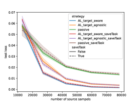
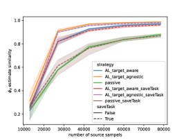
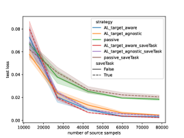
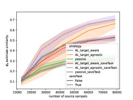
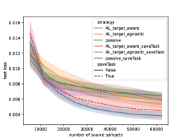
Figure 3: Results on synthetic data with 8000 target sample Left side presents the test loss and the right side presents the similarity between the column space of the ground truth $\phi_{X}$ and the estimated $\hat{\phi}_{X}$. Notice that how to measure the similarity on neural networks is unclear so we skip this result. Top and middle: Results of the nonlinear kernel. The target-aware AL gets the lowest test loss while the passive gets the highest. In terms of saveTask, we notice that reducing task switch number does not affect the performance a lot. From the left figure, the target-agnostic AL gets the best estimation which aligns with our design intuition that target-agnostic AL should have a universal good estimation in all directions. It is a little surprising to us that the passive one performs worst. We conjecture the reason that the GD-based oracle is not that good for joint-task training and should again have better performance when using [12, 10]. Bottom: Result of non-linear representation. Here we notice that the saving task strategy leads to slightly worse performance. While the target-aware AL still gives the worst test loss, the difference between passive and target-agnostic AL is small due to the complexity of the shallow net.

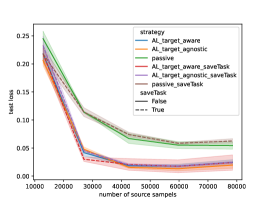
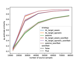
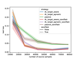
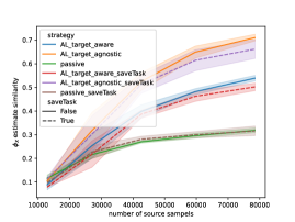
Figure 4: Results on synthetic data with 800 target sample Top and middle: The bilinear and nonlinear $\psi_{X}$ case gives a similar performance as before. Bottom: For $\phi_{W}$ as a neural net, we notice here the AL does not show an advantage until the very end where the passive stops decreasing. This may suggest for nonlinear representation, more target data may be needed for a beneficial source selection compared to the bilinear $\phi$.

D.2 Pendulum simulator

D.2.1 Settings

Data generation

We consider the following continuous-time pendulum dynamics model adopted from [23]:

$$ml^{2}\ddot{\theta}-ml\hat{g}\sin\theta=u+f(\theta,\dot{\theta},w)$$

where $\theta,\dot{\theta},\ddot{\theta},u$ are angle, angular velocity, angular acceleration, and control, $m,l,\hat{g}$ are mass, pole length, and the gravity estimation, and finally, $f$ is the unknown residual dynamics term to be learned with $w$ the environment parameter. The ground truth $f$ is given by

$$F=\|R\|_{2}^{2}\cdot R,R=c-\left[\begin{array}[]{c}l\dot{\theta}\cos\theta\\ -l\dot{\theta}\sin\theta\end{array}\right]$$

$$f(\theta,\dot{\theta},w) =\underbrace{\vec{l}\times F}_{\text{air drag }}-\underbrace{\alpha_{1}\dot{\theta}-\alpha_{2}\dot{\theta}|\dot{\theta}|}_{\text{damping }}+\underbrace{ml(g-\hat{g})\sin\theta}_{\text{gravity mismatch }}$$

$$w=[c_{x},c_{y},\alpha_{1},\alpha_{2},\hat{g},0\text{ or }1]$$

where $c=[c_{x},c_{y}]$ is external wind, $\alpha_{1},\alpha_{2}$ are damping coefficients and $g$ is the true gravity.

We let $x=[\theta,\dot{\theta}]$ denote the input to $f$. Notice here the last element of $w$ is a dummy feature. For the source tasks, we always have $w[6]=0$ since all the source parameters are known. For the single target task, we have $w_{\text{actual\_target}}$ to generate the data, so $w_{\text{actual\_target}}[6]=0$. But the learner only observes the $w_{\text{target}}=[0,0,0,0,0,1]$, which indicates the unknown environment of the target. In the simulator, we collect data using a stochastic policy to approximate i.i.d. data distribution.

It is easy to see that $f$ is highly nonlinear regarding $x,w$. Therefore we use the known nonlinear feature operator $\psi$ to make it close to the linear model with some misspecification:

$$\psi_{X}\text{ is the Fourier feature kernel which has been defined in the synthetic data section}$$

$$\psi_{W}(w)=[l_{x},l_{y},g,\alpha_{1},\alpha_{2},CxCy,Cx^{2},Cx^{2}C_{y},C_{x}^{3},Cy^{2},Cy^{2}C_{x},C_{y}^{3},0\text{ or }1]$$

Other common parameters are specified in Table. 4.

target number	$d_{X}$	$d_{\psi_{X}}$	$d_{W}$	$d_{\psi_{W}}$	$k$	$\phi$ structure	inputs distribution	label noise variance
4000	2	60	13	6	8	bilinear	(See details above)	0.5

Table 4: Model parameters for pendulum simulator.

Training models and optimizer

We again use the bilinear model. For the training methods, we first do joint-GD as before using AdamW with $lr=0.01,wd=0.05,\text{batch\_size}=512$. Then after joint training, we freeze the $\phi_{X}$ parts and only trained on the targets to get the non-shared embed $\phi_{W}(w_{\text{target}})$. Another modification is that, since we are in the misspecification setting, using data collected in stage 3 might amplify the errors when estimating the target-related source. To tackle this negative transfer learning, we only use the data collect from stage 2 in previous the epochs to compute $q_{3}$. While in the synthetic data, all data, including one from stage 3, collected in previous epochs can be used.

Detailed implementation for AL strategy

The input space ${\mathcal{X}}$ and task space ${\mathcal{W}}$ of this pendulum data again lie perfectly in a ball after some normalization. Nevertheless, the underlying model is no longer linear in terms of $w$, which adds some extra difficulties to the optimal design on $w$. Here we use the adaptive sampling methods mentioned in the main paper. That is, we will iteratively sample from ${\mathcal{W}}_{\text{source}}$ and find the ones that minimize follows.

$$\min_{\{w_{i}\}\in{\mathcal{W}}_{\text{source}}}\|\hat{B}_{W,j}^{\text{source}}\psi_{W}(w_{i})-u_{i}\sqrt{\lambda_{i}}\|$$

where $u_{i}\sqrt{\lambda_{i}}$ is defined in line 9. Other parts of the algorithm can still be implemented as in the synthetic data section.

Using learned $f$ for control

To show that a better dynamics model can transfer to better control performance, we deploy the following nonlinear controller $\pi(x,\hat{f})$ as a function of $\hat{f}$ (prediction result of $f$ in the target task):

$$u=-ml\hat{g}\sin\theta-\hat{f}(\theta,\dot{\theta})-ml^{2}(K_{P}\theta+K_{D}\dot{\theta})$$

Here we focus on the regulation task, i.e., $\|x\|\rightarrow 0$. It is worth noting that the above controller is guaranteed to be exponentially stable: $\|x\|\rightarrow\eta$ exponentially fast, where $\eta$ is an error ball whose size is proportional to $\|f-\hat{f}\|_{\infty}$.

D.2.2 Results

In the main paper, we use the unobservable actual target as $[0,0,1,0.5,0,0]$. Here we give more results in Figure. 5

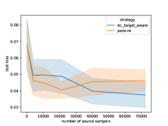
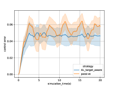
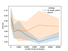
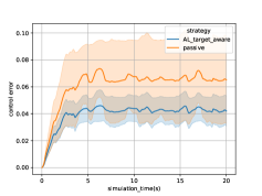
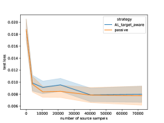
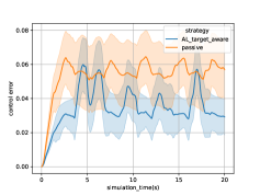
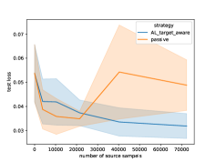
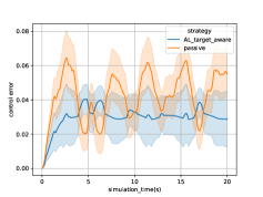
Figure 5: Results on pendulum simulator for a specific target. Left: The test loss of the estimated model $\hat{f}$. The passive strategy suffers from negative transfer while the active strategy steadily decreases. Right: The control error using final output $\hat{f}$. Here we use a model-based nonlinear policy $\pi(x,\hat{f})$. The model learned from active strategy leads to better control performance. From top to bottom, we have the unobservable $w_{\text{actual\_target}}$ as $[0,0,0.5,0,0.5,0],[0,0,1,1,-1,0],[0,-1,0.5,0,0.5,0],[0,0.1,0,-1,0.5,0]$. Overall, although AL does not always have a dominating advantage, most times it is more stable and can gain better test loss at the end.

D.3 Real-world drone flight dataset

D.3.1 Settings

The training model and optimizer

Here we use two layer MLP model as specified below. For the training methods, we do joint-GD as before using AdamW with $lr=0.005$ and batch_size$=1000$. Other common parameters are specified in Table. 5.

target number	$d_{X}$	$d_{\psi_{X}}$	$d_{W}$	$d_{\psi_{W}}$	$k$	$\phi$ structure
500	11	11	18 one-hot	18	2	MLP with hidden layers $[11,2]$

Table 5: Model parameters for drone dataset.

Data generation

We use the same data as stated in the main paper.

Detailed implementation for AL strategy

Unlike the previous two settings where the task space ${\mathcal{W}}$ is continuous, here we consider a discrete task space. Therefore the Algo. 2 no longer works. Therefore, here we use a similar technique as the Algorithm proposed in [8], which can be seen as a special case under the general Algo. 1. We want to emphasize that this choice is due to the limitation of real-world datasets, i.e., we can not arbitrarily query $w$ to sample, and the main purpose is to show the potential of such a framework in real-world robotics applications.

D.3.2 Results

In the main paper, we provide the result when assuming a bilinear underlying model. Here we further show the effectiveness of our methods under nonlinear $\phi_{X}$.

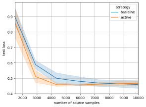
Figure 6: Results on the real drone dataset with target drone_type_A_30_z by using a neural net model. Our active strategy could converge faster than the passive strategy in the neural net model setting. Active strategy is able to converge faster than uniform sampling with smaller variances in the latter stage.

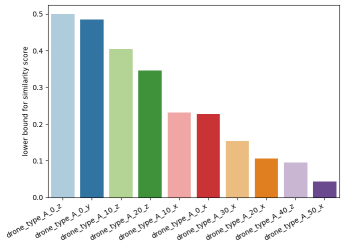
Figure 7: Top 10 the most similar source tasks. Again, given the target environment, the algorithm successfully finds the other drone_type_A environments as relevant sources, which aligns with our observation in the main paper.

References

- Shi et al. [2019] Guanya Shi, Xichen Shi, Michael O’Connell, Rose Yu, Kamyar Azizzadenesheli, Animashree Anandkumar, Yisong Yue, and Soon-Jo Chung. Neural lander: Stable drone landing control using learned dynamics. In 2019 International Conference on Robotics and Automation (ICRA), pages 9784–9790. IEEE, 2019.
- Lee et al. [2020] Joonho Lee, Jemin Hwangbo, Lorenz Wellhausen, Vladlen Koltun, and Marco Hutter. Learning quadrupedal locomotion over challenging terrain. Science robotics, 5(47):eabc5986, 2020.
- Radford et al. [2021] Alec Radford, Jong Wook Kim, Chris Hallacy, Aditya Ramesh, Gabriel Goh, Sandhini Agarwal, Girish Sastry, Amanda Askell, Pamela Mishkin, Jack Clark, et al. Learning transferable visual models from natural language supervision. arXiv preprint arXiv:2103.00020, 2021.
- Brown et al. [2020] Tom B Brown, Benjamin Mann, Nick Ryder, Melanie Subbiah, Jared Kaplan, Prafulla Dhariwal, Arvind Neelakantan, Pranav Shyam, Girish Sastry, Amanda Askell, et al. Language models are few-shot learners. arXiv preprint arXiv:2005.14165, 2020.
- Yu et al. [2022] Jiahui Yu, Zirui Wang, Vijay Vasudevan, Legg Yeung, Mojtaba Seyedhosseini, and Yonghui Wu. Coca: Contrastive captioners are image-text foundation models. arXiv preprint arXiv:2205.01917, 2022.
- Alayrac et al. [2022] Jean-Baptiste Alayrac, Jeff Donahue, Pauline Luc, Antoine Miech, Iain Barr, Yana Hasson, Karel Lenc, Arthur Mensch, Katherine Millican, Malcolm Reynolds, et al. Flamingo: a visual language model for few-shot learning. Advances in Neural Information Processing Systems, 35:23716–23736, 2022.
- O’Connell et al. [2022] Michael O’Connell, Guanya Shi, Xichen Shi, Kamyar Azizzadenesheli, Anima Anandkumar, Yisong Yue, and Soon-Jo Chung. Neural-fly enables rapid learning for agile flight in strong winds. Science Robotics, 7(66):eabm6597, 2022.
- Chen et al. [2022] Yifang Chen, Kevin Jamieson, and Simon Du. Active multi-task representation learning. In International Conference on Machine Learning, pages 3271–3298. PMLR, 2022.
- Du et al. [2021] Simon S. Du, Wei Hu, Sham M. Kakade, Jason D. Lee, and Qi Lei. Few-shot learning via learning the representation, provably, 2021.
- Tripuraneni et al. [2020] Nilesh Tripuraneni, Michael I. Jordan, and Chi Jin. On the theory of transfer learning: The importance of task diversity, 2020.
- Tripuraneni et al. [2021] Nilesh Tripuraneni, Chi Jin, and Michael Jordan. Provable meta-learning of linear representations. In International Conference on Machine Learning, pages 10434–10443. PMLR, 2021.
- Thekumparampil et al. [2021] Kiran Koshy Thekumparampil, Prateek Jain, Praneeth Netrapalli, and Sewoong Oh. Sample efficient linear meta-learning by alternating minimization. arXiv preprint arXiv:2105.08306, 2021.
- Xu and Tewari [2021] Ziping Xu and Ambuj Tewari. Representation learning beyond linear prediction functions. Advances in Neural Information Processing Systems, 34:4792–4804, 2021.
- Collins et al. [2022] Liam Collins, Aryan Mokhtari, Sewoong Oh, and Sanjay Shakkottai. Maml and anil provably learn representations. In International Conference on Machine Learning, pages 4238–4310. PMLR, 2022.
- Rahimi and Recht [2008] Ali Rahimi and Benjamin Recht. Uniform approximation of functions with random bases. In 2008 46th annual allerton conference on communication, control, and computing, pages 555–561. IEEE, 2008.
- Todd [2016] Michael J Todd. Minimum-volume ellipsoids: Theory and algorithms. SIAM, 2016.
- Akimoto et al. [2012] Youhei Akimoto, Yuichi Nagata, Isao Ono, and Shigenobu Kobayashi. Theoretical foundation for cma-es from information geometry perspective. Algorithmica, 64:698–716, 2012.
- Raghu et al. [2019] Aniruddh Raghu, Maithra Raghu, Samy Bengio, and Oriol Vinyals. Rapid learning or feature reuse? towards understanding the effectiveness of maml. arXiv preprint arXiv:1909.09157, 2019.
- Nichol and Schulman [2018] Alex Nichol and John Schulman. Reptile: a scalable metalearning algorithm. arXiv preprint arXiv:1803.02999, 2(3):4, 2018.
- Antoniou et al. [2018] Antreas Antoniou, Harrison Edwards, and Amos Storkey. How to train your maml. arXiv preprint arXiv:1810.09502, 2018.
- Hospedales et al. [2021] Timothy Hospedales, Antreas Antoniou, Paul Micaelli, and Amos Storkey. Meta-learning in neural networks: A survey. IEEE transactions on pattern analysis and machine intelligence, 44(9):5149–5169, 2021.
- Chen et al. [2021] Shuxiao Chen, Koby Crammer, Hangfeng He, Dan Roth, and Weijie J. Su. Weighted training for cross-task learning, 2021.
- Shi et al. [2021] Guanya Shi, Kamyar Azizzadenesheli, Michael O’Connell, Soon-Jo Chung, and Yisong Yue. Meta-adaptive nonlinear control: Theory and algorithms. Advances in Neural Information Processing Systems, 34:10013–10025, 2021.