Spatial modeling of extremes and an angular component

Abstract

Many environmental processes such as rainfall, wind or snowfall are inherently spatial and the modeling of extremes has to take into account that feature. In addition, environmental extremes are often attached with an angle, e.g., wind gusts and direction or extreme snowfall and time of occurrence. This article proposes a Bayesian hierarchical model with a conditional independence assumption that aims at modeling simultaneously spatial extremes and angles. The proposed model relies on the extreme value theory as well a recent development for handling directional statistics over a continuous domain. Starting with sketches of the necessary elements of extreme value theory and directional statistics, the model is motivated. Working within a Bayesian setting, a Gibbs sampler is introduced and whose performances are analyzed through a simulation study. The paper ends with an application on extreme snowfalls in the French Alps. Results show that, the most severe events tend to occur later in the snowfall season for high elevation regions than for lower altitudes.

Keywords: Extreme value theory, Spatial extremes, Circular statistics, Bayesian hierarchical models, Markov Chain Monte Carlo, Environmental application

1 Introduction

Natural hazards may cause severe damages or economic losses such as floods or heatwaves. Extreme snowfalls are not an exception as large amount of snow may damage buildings due to excessive mass or put population at risk due to avalanches. To prevent such catastrophic events, European policies impose that buildings must be designed to face the 50–year return level and snowshed the 100–years return level. The main difficulty in modeling extreme snowfalls is that, as many environmental processes, e.g., temperature, rainfall, it is spatial in extent. Fortunately, the last decade has seen many theoretical developments as well as extensive applications to try to analyze spatial extremes. From a probabilistic point of view, the relevant framework for modeling extreme events is the extreme value theory whose focus is precisely on the tail of the distribution. One widely used approach for analyzing spatial extremes is through max-stable processes (de Haan and Fereira,, 2006; Davison and Gholamrezaee,, 2011; Davison et al.,, 2013) as they appear as the only non degenerate limit of pointwise maxima over independent copies of stochastic processes—after an appropriate affine normalization. Recent works about max-stable processes involve inferential frameworks (Padoan et al.,, 2010; Ribatet et al.,, 2012; Huser et al.,, 2019), (exact) simulations (Schlather,, 2002; Oesting et al.,, 2012; Dombry et al.,, 2016), conditional simulations (Dombry et al.,, 2013) or non stationary dependence structures (Huser and Genton,, 2016; Richards and Wadsworth,, 2021).

However, inference from max-stable processes is challenging as the associated (full) likelihood is too CPU demanding or even numerically intractable (Dombry et al.,, 2017; Huser et al.,, 2019). Even if the above computational cost may be avoided within a Bayesian setting combined with a composite likelihood approach, it would result in a non standard inferential framework (Ribatet et al.,, 2012). Consequently and, as long as pointwise prediction is of concern, as opposed to areal quantities such as accumulated snowfall over a spatial domain $\mathcal{X}\subset\mathbb{R}^{d}$, $d\geq 1$, one can restrict our attention to the univariate case for which extreme value theory justifies the use of the Generalized Extreme Value distribution (GEV) whose cumulative distribution function is

$$\Pr\{\eta(s)\leq z\}=\exp\left[-\left\{1+\xi(s)\frac{z-\mu(s)}{\sigma(s)}\right\}^{-1/\xi(s)}\right],\qquad 1+\xi(s)\frac{z-\mu(s)}{\sigma(s)}>0,$$ (1)

where $\eta(s)$ denotes the block maxima random variable at location $s\in\mathcal{X}$, and $\mu(s)\in\mathbb{R}$, $\sigma(s)\in(0,\infty)$, $\xi(s)\in\mathbb{R}$ are respectively the location, scale and shape GEV parameters.

Although in general we can, based on some covariates $\mathbf{x}(s)$, place any regression structures for the GEV parameters, e.g., $\mu(s)=f_{\mu}\{\mathbf{x}(s);\boldsymbol{\beta}_{\mu}\}$, most of the applications have been restricted to the linear setting, e.g., $f_{p}(\mathbf{x}(s);\boldsymbol{\beta}_{p})=\beta_{0,p}+\mathbf{x}^{\top}(s)\boldsymbol{\beta}_{p}$, $p\in\{\mu,\sigma,\xi\}$ (Davison and Gholamrezaee,, 2011; Padoan et al.,, 2010). The advantage of the linear assumption is that joint estimation of both the spatial dependence and the regression parameters is rather straightforward. However in many situations it is too restrictive and yield to unrealistically smooth surfaces unable to catch the natural spatial variability of extremes (Davison et al.,, 2012).

To bypass this hurdle, one can take benefit of using a latent hierarchical model with a conditional independence assumption (Cooley et al.,, 2007) where the GEV parameters now vary spatially according to some stochastic process, i.e.,

$$\eta(s)\mid\{\mu(s),\sigma(s),\xi(s)\} \stackrel{{\scriptstyle\text{ind}}}{{\sim}}\mbox{GEV}\{\mu(s),\sigma(s),\xi(s)\},\qquad s\in\mathcal{X}$$ (2)

$$\mu(\cdot) \sim\mbox{GP}(m_{\mu},\gamma_{\mu})$$

$$\sigma(\cdot) \sim\mbox{GP}(m_{\sigma},\gamma_{\sigma})$$

$$\xi(\cdot) \sim\mbox{GP}(m_{\xi},\gamma_{\xi})$$

where $\mbox{GP}(m,\gamma)$ denotes a (univariate) Gaussian process with mean function $m\colon s\mapsto m(s)$ and covariance function $\gamma\colon(s_{1},s_{2})\mapsto\gamma(s_{1},s_{2})$ and the above three Gaussian processes are usually assumed independent for simplicity.

Often though not invariably, focus is not only extreme values but also on an “angular component” such as the orientation of wind gusts. Moreover, a conventional extreme value analysis completely ignores the time of occurrence of records, although it may be a valuable quantity. The latter can often be represented as an angle. To the best of our knowledge, little attention have been paid to the joint modeling of extreme and such an angular component. This paper aims at filling this gap by considering a hierarchical Bayesian framework which takes advantage of the previous conditional independence assumption and handle both the extremal and angular aspect of the data. The paper is organized as follows. Section 2 recalls the basic theory for handling the specificity of directional data and Section 3 extends the theory to the spatial setting by introducing the projected Gaussian process model. Section 4 introduces the proposed approach and details how inference can be done using MCMC techniques. Section 5 gives a simulation study while Section 6 applies the proposed methodology to extreme snowfalls in the French Alps. The paper ends with a discussion. Specific details on MCMC implementation are deferred to the appendix.

2 Directional statistics

At the end of the 1960’s and since applications dealing with angular variable data sets was increasingly more popular, there was a pressing need to develop a theoretical framework for the statistical modeling of angles. A comprehensive review of directional statistics can be found in Mardia and Jupp, (2009). In this section, we will present the basic concepts of this theory, in order to motivate the statistical model used for the angular component of our model.

A random angle $\theta$ is characterized by a probability density function $f$ defined on $[0,2\pi]$ but extended to $\mathbb{R}$ such that $f(x+2\pi)=f(x)$ for all $x\in\mathbb{R}$. The usual quantities such as the (Cartesian) mean or standard deviation are not well defined and need to be redefined. Their angular counterparts can be found thanks to the characteristic function $\phi\colon t\mapsto\mathbb{E}\left\{\exp(itX)\right\}$. Taking $t=1$, we get $\phi(1)=\rho e^{i\mu}$, where $\mu$ is known as the mean direction and $\rho$ as the mean resultant length.

Having observed a sample of angles $\theta_{1},\ldots,\theta_{n}$, we can define points on the unit circle $\mathbb{S}^{1}=\{x\in\mathbb{R}^{2}\colon\|x\|_{2}=1\}$, i.e., $x_{i}=\{\cos\theta_{i},\sin\theta_{i}\}^{\top}$, $i=1,\ldots,n$. The empirical mean direction, denoted $\bar{\theta}_{n}$, is thus defined as the projection of the empirical (Cartesian) mean $\bar{x}_{n}=(\bar{x}_{n,1},\bar{x}_{n,2})=n^{-1}\sum_{i}x_{i}$ onto $\mathbb{S}^{1}$

$$\bar{\theta}_{n}=\arctan^{*}\left(\frac{\bar{x}_{n,2}}{\bar{x}_{n,1}}\right),\qquad\arctan^{*}\left(\frac{y}{x}\right)=\begin{cases}\arctan(y/x),&\text{if $x>0$}\\ \text{sign}(y)\pi/2,&\text{if $x=0$}\\ \arctan(y/x)+\pi,&\text{if $x<0$}\end{cases}$$

The sample mean resultant length is $\bar{R}_{n}=\|\bar{x}_{n}\|_{2}$ from which one can define an important measure of dispersion $V=\sqrt{1-\bar{R}_{n}}$. Under mild regularity conditions, it can be shown that both statistics $\bar{\theta}_{n}$ and $\bar{R}_{n}$ are consistent and asymptotically Gaussian whose covariance matrix is fully characterized but not presented here (see Mardia and Jupp, (2009), page 76).

We now introduce some widely used parametric statistical models for angular data, namely the Von Mises, wrapped and projected distributions.

The Von Mises distribution, denoted $M(\mu,\kappa)$, plays a central role in circular statistics and, in some sense, is the analogue of the Gaussian distributions for angular distribution/ In particular, the Von Mises distribution is the maximum entropy distribution on the circle with mean direction $\mu$ and mean resultant length $\rho$. Its probability density function is

$$f(x;\mu,\kappa)=\frac{1}{2\pi I_{0}(\kappa)}\exp\left\{\kappa\cos(x-\mu)\right\},\qquad x\in[0,2\pi],$$

where $I_{0}$ denotes the modified Bessel function of the first kind and order 0.

However in concrete applications, von Mises distributions are of limited interest since they are always unimodal and symmetric. Although some generalization of the Von Mises distribution have been proposed such as Mardia and Spurr, (1973) or Cox, (1975), none of them allowed for multivariate or spatial extensions.

Another family of angular distributions is wrapped distributions. A wrapped distribution is obtained by taking any probability density function $g$ defined on $E\subseteq\mathbb{R}$ and wrapping it on $[0,2\pi]$, i.e., the associated probability density function is

$$f(x)=\sum_{k=-\infty}^{\infty}g(x+2k\pi)1_{\{x+2k\pi\in E\}}.$$ (3)

Contrary to Von Mises distributions and since wrapped distributions inherit the properties of the underlying probability density function $g$, various shapes for the density are possible such as multimodality and asymmetry. The main drawback is that inference from this model is usually difficult. Indeed, since the density is defined as a sum of densities, computing the maximum likelihood estimator is not straightforward and is typically treated as a missing data problem where the interval index $k$ in (3) is treated as a latent variable. Consequently, it is common practice to fit this model using EM or Monte-Carlo Markov-Chain algorithms. Further extensions to the multivariate or spatial cases is even more complicated since one would have to define a integer valued random vector / spatial process, e.g., $\{k(s)\colon s\in\mathcal{X}\}$, which is far from being easy.

Similarly to wrapped distributions, projected distributions are obtained from an underlying probability density function $g$ which in this case is defined on $E\subseteq\mathbb{R}^{2}$. Let $\mathbb{X}=(X_{1},X_{2})^{\top}$ be a random vector drawn from $g$. The associated random angle $\theta$ is defined as the projection of $\mathbb{X}$ onto the unit circle $\mathbb{S}^{1}$, i.e., $\theta=\arctan^{*}(X_{2}/X_{1})$. We thus have $X=(R\cos\theta,R\sin\theta)$ and it can be shown that $\theta$ has density

$$f(x)=\int_{0}^{\infty}rg(r\cos x,r\sin x)\mbox{d$r$},\qquad x\in[0,2\pi].$$

Similarly to wrapped distributions, projected distributions are very flexible and several modes as well as asymmetry are possible. A specific case of particular importance is to use a Gaussian vector with mean $\mu$ and covariance matrix $\Sigma$ for $X$ (Gelfand and Wang,, 2013). The main advantage of using the Gaussian assumption is that it easily extends to the spatial case by substituting the Gaussian random vector for a Gaussian random field. Gelfand and Wang, (2014) proposed an inferential framework for this case where they treated the radius $R$ as a latent variable. In doing so it is therefore possible to make use of the Gaussian likelihood on $\mathbb{X}=(R\cos\theta,R\sin\theta)$.

3 The projected Gaussian process model

In this section, we give a more complete overview about the projected Gaussian process model. Let $\{\mathbb{X}(s)=\{X_{1}(s),X_{2}(s)\}^{\top}\colon s\in\mathcal{X}\}$ be a bivariate Gaussian process defined on the spatial domain $\mathcal{X}\subset\mathbb{R}^{d}$, $d\geq 1$, with mean function $\mu\colon s\mapsto\mathbb{E}[\mathbb{X}(s)]$ and covariance function $\gamma\colon(s_{1},s_{2})\mapsto\Gamma$ where $\Gamma$ is a $4\times 4$ block-matrix with each block $\Gamma_{i,j}=\mbox{Cov}\{X(s_{i}),X(s_{j})\}$, $i,j=1,2$. Based on the above bivariate Gaussian process, we can define the projected Gaussian process $\{\theta(s)=\arctan^{*}\{X_{2}(s)/X_{1}(s)\}\colon s\in\mathcal{X}\}$, denoted $\theta\sim PG\{\mu,\gamma\}$, with underlying mean and covariance functions $\mu$ and $\gamma$ respectively. For any $s\in\mathcal{X}$, it can be shown that the probability density function of $\theta(s)$ is

$$f_{s}(x)=\frac{\phi_{2}\left(\mathbb{\mu}(s);0,\gamma(s,s)\right)+|\gamma(s,s)|^{-1/2}D(x)\Phi_{1}(D(x))\phi_{1}\left(a_{s}(x)^{-1}|\gamma(s,s)|^{-1/2}\mathbb{\mu}(s)\wedge\mathbf{u}(x)\right)}{a_{s}^{2}(x)}$$

where $\phi_{1}$ and $\Phi_{1}$ denote the standard normal density and distribution respectively, $\phi_{2}(\cdot;0,\Sigma)$ the density of a centered bivariate Gaussian vector with covariance matrix $\Sigma$, $\mathbf{u}(x)=(\cos x,\sin x)^{\top}$, $a_{s}^{2}(x)=\mathbf{u}(x)^{\top}\gamma(s,s)^{-1}\mathbf{u}(x)$ and $D(x)=a_{s}(x)^{-1}\mathbb{\mu}(s)^{\top}\gamma(s,s)^{-1}\mathbf{u}(x)$ (see Mardia, (1972), page 52).

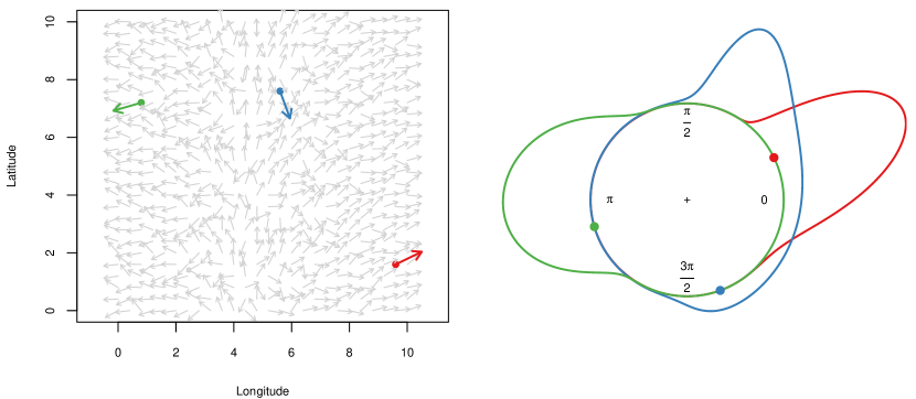
Figure 1: Illustration of the projected Gaussian process. Left: Realization of a projected Gaussian process with three highlighted locations (colored arrows). Right: projected Gaussian densities at the three highlighted locations. Each blob corresponds to the observed directions

The above formula is rather complex and does not generalize well in a spatial setting. However, it is possible to work within an augmented data framework by considering a radial latent process $\{R(s)\colon s\in\mathcal{X}\}$. More precisely, for some spatial locations $\mathbf{s}=(s_{1},\ldots,s_{k})\in\mathcal{X}^{k}$, $k\geq 1$, we associate to the the angular random vector $\boldsymbol{\theta}(\mathbf{s})=\{\theta(s_{1}),\ldots,\theta(s_{k})\}$ a radial random vector $\mathbf{R}(\mathbf{s})=\{R(s_{1}),\ldots,R(s_{k})\}$ so that one can easily switch from polar coordinates $\{\mathbf{R}(\mathbf{s}),\boldsymbol{\theta}(\mathbf{s})\}$ to Cartesian ones $\mathbf{X}(\mathbf{s})=\{\mathbf{R}(\mathbf{s})\cos\boldsymbol{\theta}(\mathbf{s}),\mathbf{R}(\mathbf{s})\sin\boldsymbol{\theta}(\mathbf{s})\}$, where multiplication is done componentwise. Figure 1 plots one realization of the projected Gaussian process.

Inference is therefore based on the induced bivariate Gaussian random vector $\mathbf{X}(\mathbf{s})$ and it is easily seen that, for any $\mathbf{r}\in(0,\infty)^{k}$ and $\mathbf{t}\in[0,2\pi]^{k}$, the joint density of the random vector $\{\mathbf{R}(\mathbf{s}),\boldsymbol{\theta}(\mathbf{s})\}$ is

$$f_{\mathbf{s}}(\mathbf{r},\mathbf{t})=(2\pi)^{-k/2}|\Sigma(\mathbf{s})|^{-1/2}\exp\left(-\frac{\{\mathbf{r}^{\top}\mathbf{u}-\boldsymbol{\mu}(\mathbf{s})\}^{\top}\Sigma(\mathbf{s})^{-1}(\mathbf{r}^{\top}\mathbf{u}-\boldsymbol{\mu}(\mathbf{s})\}}{2}\right)\prod_{i=1}^{k}r_{i},$$ (4)

with

$$\mathbf{u}=\begin{bmatrix}\cos t_{1}&\ldots&\cos t_{k}\\ \sin t_{1}&\ldots&\sin t_{k}\end{bmatrix}^{\top},$$

and where $\boldsymbol{\mu}(\mathbf{s})$ and $\Sigma(\mathbf{s})$ are respectively the mean vector and cross-covariance matrix of the Gaussian random vector $\mathbf{X}(\mathbf{s})$.

4 Extreme–angular Bayesian hierarchical model

Figure 2: Directed acyclic graph for the extreme–angular hierarchical model with the latent radial process $\{R(s)\colon s\in\mathcal{X}\}$. A double arrow indicates a deterministic relationship between the two nodes.

Based on the latent variable for extremes introduced in (2) and that proposed by Gelfand and Wang, (2013) for angular data described in Section 3, one can define what we shall call a spatial extreme–angular Bayesian hierarchical model that merges the two previous approaches. More precisely the model is now given by

$$\theta(\cdot)\mid\{m_{\theta},\gamma_{\theta},\mu(\cdot),\sigma(\cdot),\xi(\cdot)\} \sim\mbox{PG}(m_{\theta},\gamma_{\theta}),$$ (5)

$$\eta(s)\mid\{\mu(s),\sigma(s),\xi(s)\} \stackrel{{\scriptstyle\text{ind}}}{{\sim}}\mbox{GEV}\{\mu(s),\sigma(s),\xi(s)\},\qquad s\in\mathcal{X}$$

$$\mu(\cdot)\mid\{m_{\mu},\gamma_{\mu}\} \sim\mbox{GP}(m_{\mu},\gamma_{\mu})$$

$$\sigma(\cdot)\mid\{m_{\sigma},\gamma_{\sigma}\} \sim\mbox{GP}(m_{\sigma},\gamma_{\sigma})$$

$$\xi(\cdot)\mid\{m_{\xi},\gamma_{\xi}\} \sim\mbox{GP}(m_{\xi},\gamma_{\xi})$$

where prior distributions are put on the mean and covariance function parameters on each (projected) Gaussian processes. The last 4 lines are identical to model (2). Further, as suggested by the conditioning terms, the mean function for the angular process may depend on spatial covariates such as longitude, latitude or elevation but also on the GEV parameters $\mu(\cdot)$, $\sigma(\cdot)$ and $\xi(\cdot)$. Figure 2 gives the directed acyclic graph for this model.

As far as inference is of concern and due to the presence of latent variables, the likelihood has an integral representation, i.e., marginalization over the latent variables, and therefore the likelihood has no closed form. Since we are working in a Bayesian setting, marginalization across the latent variables is done numerically using MCMC techniques, e.g., Gibbs sampler. However compared to the original model (2), an extra difficulty arises to handle appropriately the angular spatial process whose finite dimensional distributions have no explicit forms. In the same vein as the latent variable approach of Gelfand and Wang, (2014), we add an additional random field $\{R(s)\colon s\in\mathcal{X}\}$ that represents a radius over the spatial domain $\mathcal{X}$. Consequently by including the latent radial process, it is possible to easily switch from the polar coordinates $\{(R(s),\theta(s))\colon s\in\mathcal{X}\}$ to the Cartesian ones $\{X(s)=(R(s)\cos\theta(s),R(s)\sin\theta(s))\colon s\in\mathcal{X}\}$ and conversely. Contrary to the polar coordinates, working in the Cartesian system is straightforward as one can rely on the density of a bivariate Gaussian random field.

A Gibbs sampler for model (5) consists in sampling sequentially from the following full conditional distributions. The update of the GEV latent processes parameters is done by sampling from

$$\pi(m_{\mu}\mid\ldots)\propto\pi\{\mu(\mathbf{s})\mid m_{\mu}(\mathbf{s}),\gamma_{\mu}(\mathbf{s},\mathbf{s})\}\pi(m_{\mu})$$

with a slight abuse of notation where $\pi(m_{\mu}\mid\ldots)$ denotes the full conditional distribution of parameters of the mean function of the GEV location parameters and $\pi(m_{\mu})$ the associated prior distribution. Similar expressions are found for the mean function of the GEV scale and shape parameters as well as for the parameters of the covariance functions $\gamma_{\mu}$, $\gamma_{\sigma}$ and $\gamma_{\xi}$.

The update of the latent GEV parameters is done by sampling from

$$\pi\{\mu(s_{j})\mid\ldots)\propto\prod_{i=1}^{n}\pi\{\eta_{i}(s_{j})\mid\mu(s_{j}),\sigma(s_{j}),\xi(s_{j})\}\pi\{X_{i}(\mathbf{s})\mid m_{\theta},\gamma_{\theta},\mu(\mathbf{s}),\sigma(\mathbf{s}),\xi(\mathbf{s})\}\pi\{\mu(\mathbf{s})\mid m_{\mu},\gamma_{\mu}\},$$

for $j=1,\ldots,k$ and with similar expressions for the scale and shape GEV latent processes.

Updating the angular process parameters is a bit more involved and, as mentioned in Section 3, relies on data augmentation with a radial random field to allow for the use of a Gaussian likelihood. More precisely we update the latent radius process by sampling from

$$\pi\{R_{i}(\mathbf{s})\mid\ldots\}\propto\pi\{R_{i}(\mathbf{s})\mid\theta_{i}(\mathbf{s}),m_{\theta},\gamma_{\theta},\mu(\mathbf{s}),\sigma(\mathbf{s}),\xi(\mathbf{s})\},\qquad i=1,\ldots,n,$$

where, in the implementation of the sampler, the above conditional density is actually computed using (4).

Finally, the projected Gaussian processes parameters are updated as parameters of a bivariate Gaussian process with completed observed data $\{\mathbf{X}(s)=(R(s)\cos\theta(s),R(s)\sin\theta(s))\colon s\in\mathcal{X}\}$. We have

$$\pi(m_{\theta}\mid\ldots)\propto\prod_{i=1}^{n}\pi\{\mathbf{X}_{i}(\mathbf{s})\mid m_{\theta},\gamma_{\theta},\mu(\mathbf{s}),\sigma(\mathbf{s}),\xi(\mathbf{s})\}\pi(m_{\theta}),$$

where as above $\pi(m_{\theta}\mid\ldots)$ denotes the full conditional distribution of the mean function and $\pi(m_{\theta})$ is the associated prior distribution. A similar expression for the (cross) covariance function $\gamma_{\theta}$ can be found.

In practice it is convenient to make some parametric assumptions on the mean and (cross) covariance functions of the latent Gaussian processes and use conjugate prior distributions whenever possible. For instance a sensible choice for the mean function is to assume a Gaussian prior distribution and a linear form for the mean function, i.e., $m_{j}(s)=D_{j}(s)\boldsymbol{\beta}_{j}$, $j\in\{\mu,\sigma,\xi,\theta\}$, where $D_{j}(\mathbf{s})$ is the design matrix at location $s$. With this specific choice the full conditional distribution is multivariate Gaussian.

For the GEV latent processes, a parametric stationary and isotropic covariance function can be used, e.g., a powered exponential covariance $\gamma(s,s+h)=\gamma(\|h\|)=\tau\exp\left\{-\left(\|h\|/\lambda\right)^{\kappa}\right\}$. Assuming an inverse Gamma prior distribution for the sill parameter $\tau$ results in an inverse Gamma posterior distribution. However no conjugate prior distributions exist for the range and the shape parameters $\lambda$ and $\kappa$ and one has to have resort to a Metropolis–Hastings updating scheme.

For the underlying bivariate Gaussian process $\{X(s)\colon s\in\mathcal{X}\}$, a widely used parametrization is to assume a stationary isotropic and separable cross covariance function, i.e.,

$$\gamma_{\theta}(s,s+h)=\gamma_{\theta}(\|h\|)=T\otimes\rho(\|h\|),\qquad T=\begin{bmatrix}\tau_{\theta}&\rho_{\theta}\sqrt{\tau_{\theta}}\\ \rho_{\theta}\sqrt{\tau_{\theta}}&1\end{bmatrix},\qquad\tau_{\theta}>0,\quad\rho_{\theta}\in(-1,1),$$

where $\otimes$ is the Kronecker product, $\rho$ is a parametric correlation function, e.g., powered exponential, $\tau_{\theta}=\mbox{Var}\{R(s)\cos\theta(s)\}$ and $\rho_{\theta}$ is the cross component correlation, i.e., $\rho_{\theta}=\mbox{Cor}\{R(s)\cos\theta(s),R(s)\sin\theta(s)\}$, for all $s\in\mathcal{X}$. As suggested by Gelfand and Wang, (2013), we have set $\mbox{Var}\{R(s)\sin\theta(s)\}=1$ to ensure identifiability of the parameters. Specific details about the full conditional distributions are postponed to the appendix.

1

input : A Markov chain $\{\psi_{t}\colon t=1,\ldots,N\}$ sampled from the Gibbs sampler introduced above and a new location $s_{*}\in\mathcal{X}$.

2

output : Predictive posterior predictions of an unknown quantity $U(s_{*})$.

3

4for $t=1,\ldots,N$ do

       /* Conditional sampling of the GEV parameters */

5       Sample $\mu_{t}(s_{*})$ from the conditional distribution $\mu(s_{*})\mid\mu(\mathbf{s}),\psi_{t}$;

6      

7      Sample $\sigma_{t}(s_{*})$ and $\xi_{t}(s_{*})$ in the same way;

8      

      /* Conditional sampling for the angular component */

9       Sample $\theta_{t}(s_{*})$ from the conditional distribution $\theta(s_{*})\mid\mu(\mathbf{s}),\sigma(\mathbf{s}),\xi(\mathbf{s}),\psi_{t}$;

10      

11 end for

12

13Return the $U(s^{*})$-estimator $\hat{U}(\psi_{1}(s_{*}),\ldots,\psi_{N}(s_{*}))$;

14

Algorithm 1 Pointwise predictive posterior predictions from the extreme–angular model.

Spatial models often aim at predicting some unknown quantities at unobserved locations $s_{*}\in\mathcal{X}$, such as the values of the GEV parameters, the quantile of order $p$ of the GEV distribution, or the circular mode of the posterior distribution of $\theta(s^{*})$. Within a Bayesian framework, it is typically done through the posterior predictive distribution

$$\int\pi(\eta(s_{*}),\theta(s_{*})\mid\psi,\mathcal{D}_{n})\pi(\psi\mid\mathcal{D}_{n})\mbox{d$\psi$},$$

where $\mathcal{D}_{n}=\{(\eta_{i}(s_{j}),\theta_{i}(s_{j}))\colon i=1,\ldots,n,j=1,\ldots,k\}$ and $\boldsymbol{\psi}$ is the parameter vector of the model. In practice, the above integral has no closed form expressions and one has to resort to numerical integration where, as explained in Algorithm 1, each state of the generated Markov chain during the Gibbs sampler stage is browsed. When the unknown quantity $U(s_{*})$ has no closed form, one might use an empirical version of $U(s_{*})$ such as empirical quantiles of order $p$.

5 Simulation study

Table 1: Configuration settings for the simulation study. The angular mean function is set to $m_{\theta}(s)=\{m_{\theta,1}(s),m_{\theta,2}(s)\}^{\top}$. For each configuration the latent GEV parameter processes $(\mu,\sigma,\xi)$ were held fixed respectively to Gaussian processes with mean functions $m_{\mu}(s)=2-3\text{lon}(s)-2\text{lat}(s)$, $m_{\sigma}(s)=2+\text{lat}(s)$, $m_{\xi}=0.05$, sill parameters $0.1,0.5,0.05$ respectively, and range parameters $1,2,3$ respectively.

	$\sigma^{2}$	$\rho$	$m_{\theta,1}(s)$	$m_{\theta,2}(s)$	Modality
I: Independent	0.4	0.3	$0.5$	0	Multimodal
II: Smooth	0.4	0.3	$0.5$	$2\xi(s)$	Multimodal
III: Rough	1.0	0.3	$10+0.5\mu(s)$	0	Unimodal

In order to assess and the performance of our algorithm, we run a simulation study with three different extreme–angular dependence settings and let the sample size and the number of locations vary. Table 1 presents the different settings used in this simulation study. In Configuration I, the angular mean function $m_{\theta}$ is independent of the GEV parameters, so there is no connection between angles and extremes magnitude. Consequently the algorithm presented in Section 4 is equivalent to the use of two independent samplers: one for the GEV component and one for the angular component. Configuration II provides a linear dependence through the shape parameter of the GEV. However, since the Gaussian process associated to the shape parameter has a constant mean with low variance, the shape parameter has little variations over $\mathcal{X}$ and, as so, the dependence between angles and extremes magnitudes is smooth. Finally, in Configuration III the angular mean function depends on the GEV location parameter which varies significantly over $\mathcal{X}$ yielding to a strong dependence between angles and extremes magnitudes.

Working within a fixed domain framework, i.e., the spatial domain $\mathcal{X}$ is fixed, we numerically analyze two types of asymptotic: the infill asymptotic where the number of sites $k$ lying in the spatial domain $\mathcal{X}$ increases; and the large sample asymptotic where the number of replicates $n$ increases. For each dependence setting presented in Table 1, the number of spatial locations and that of replicates are respectively set to $k=10$, 25, 50 and $n=20$, 50, 100. Overall it leads to 27 possible configurations.

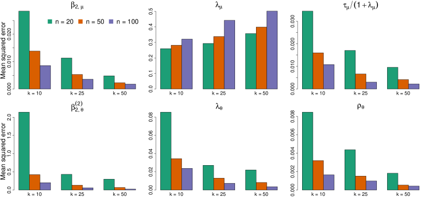
Figure 3: Evolution of the mean squared error (MSE) of parameters with varying number of observations $n$ and locations $k$ in the Smooth Configuration II. Top: MSE for the regression (left), range (middle) parameters and quotient of scale and range (right) of the covariance function of the Gaussian process $\mu$. Bottom: MSE for regression parameter (left), range parameter (middle) and correlation parameter (right) of the projected Gaussian process $\theta$.

Figure 3 shows the evolution of the mean squared error as the number of locations $k$ and replicates $n$ vary for a selected panel of parameters. The mean squared errors were computed from 100 independent experiments under the same configuration, using them as Bayesian point to estimate the posterior median. The top row of Figure 3 shows results for $\beta_{2,\mu}$, i.e., one of the regression parameters of the mean function $m_{\mu}$, $\lambda_{\mu}$, i.e., the range parameter of the covariance function $\gamma_{\mu}$ and the ratio $\tau_{\mu}/(1+\lambda_{\mu})$ where $\tau_{\mu}$ is the sill parameter. Results for other parameters and dependence configurations show similar patterns. As expected, the mean squared error for $\beta_{2,\mu}$ decreases as both $k$ and $n$ increase. Indeed, as $k$ increases, the number of GEV parameters increases and the linear structure $\mathbb{E}[\mu(s)]=x(s)^{\top}\boldsymbol{\beta}_{\mu}$ becomes more apparent. Similarly, as the number of replicates $n$ increases, the GEV parameters estimates become more accurate and the above linear structure has less noise. Interestingly, the mean squared error for $\lambda_{\mu}$ has a completely different behavior that, as stated in Zhang, (2004), is a consequence of the non identifiability of both the sill and range parameters of the exponential covariance function. Although it is not possible to jointly estimate these two parameters, Zhang, (2004) has shown that the ratio of the sill and range parameters, or equivalently $\tau/(1+\lambda)$, is identifiable. The right panel of Figure 3 corroborates this statement. Fortunately, Zhang, (2004) have shown that the non identifiability issue has no impact on the prediction of the related Gaussian process and, for our concern, accurate estimation of the GEV parameters at each location $s_{j}$ is possible. Figure 4 shows how the Markov chain is able to estimate the theoretical GEV parameters at a $s_{j}$, $j=1,\ldots,k$. The shape parameter being usually harder to estimate, we observe slightly worse performances for this parameter.

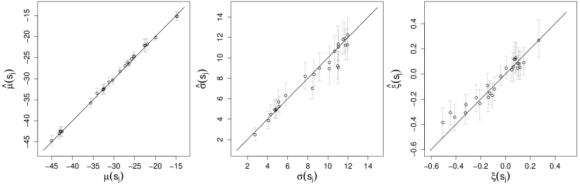
Figure 4: Posterior median estimation (with 95% credible intervals) for the GEV parameters at $k=25$ locations and with $n=50$ observations for the Smooth configuration II.

The bottom row of Figure 3 is similar to the top row, but focuses on the parameters associated to the angular component, namely $\beta_{2,\theta}^{(2)}$, $\rho_{\theta}$ and $\lambda_{\theta}$. As expected and using the same arguments as the ones stated previously, the evolution of the mean squared error $\beta_{2,\theta}^{(2)}$ is similar to that for $\beta_{2,\mu}$. There is however a subtle difference between the estimation of the parameters of the bivariate Gaussian process $\{\boldsymbol{X}(s)\colon s\in\mathcal{X}\}$ and that related to the GEV parameters, e.g., $\{\mu(s)\colon s\in\mathcal{X}\}$. In the former case, parameters are estimated from $n$ independent copies while for the latter, parameters are estimated from a single realization, i.e., for each location $s_{j}$, the GEV random variables $\eta(s_{j})$ are independent copies of a single GEV distribution. As a consequence, the sill and range parameters of the GEV Gaussian processes cannot be jointly estimated while that of the projected Gaussian process is possible.

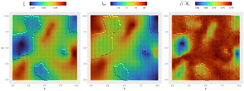
Figure 5: Prediction maps for the Smooth configuration II for 100 observations in 50 different sites. The Bayesian prediction is made via the predictive posterior distribution. Left : prediction of angle data with respect to prediction of known dependent parameter Shape. Middle : prediction of angle data with respect to estimated quantile of the extreme, with return value of 20. Right : prediction of angle data, with respect to predicted circular deviation $V=\sqrt{1-\bar{R}_{n}}$.

We now assess the predictive performance of the proposed model and, more specifically, predicting over the whole domain $\mathcal{X}$ some angular quantity of interest. As the projected Gaussian process may be multimodal, some care is needed in defining the above quantity and, in the sequel, we focus on the (main) posterior mode for the angle. Figure 7 shows prediction maps for the Smooth Configuration II where the mean function is $\mathbf{m}_{\theta}(s)=(0.5,2\xi(s))^{\top}$. With this setting, the predictive posterior distribution is bimodal and may introduce discontinuities of the predicted posterior modes. More precisely, there is a cutoff value for the shape parameter where if exceeded, the modal direction is top-right, otherwise it is bottom-right. The left panel of Figure 7 illustrates the relationship between predicted angles and shape parameters as well as the aforementioned cutoff behavior. The middle panel is similar to the previous one except that predicted quantiles of order 0.05 are now overlaid. Overall and as expected since GEV quantiles are function of the location, scale and shape parameters, the same behavior can be seen. However, since GEV quantiles is a function of all the GEV parameters, there is no deterministic relationship between quantiles and directions. For instance, quantiles in the bottom-left region are lower due to the contribution of the location parameter as opposed to the general trend “bottom-left direction for small return levels”. The right panel shows the relationship between predicted angles and the angular dispersion. One can see that the two modes have different impacts. The top–left mode is the preponderant one, and can come with a large variety of dispersion, whereas the bottom–left mode only dominates after a rare cut-off, but always is more pronounced and with less dispersion.

6 Application

Figure 6: Snowfall in the French Alps. From left to right: study region and locations of the training (blue) and validation (green) weather stations; times series of three selected training stations; empirical distribution of angles (day of year) for the three stations. The arrows point towards the sample angular mean and whose lengths are proportional to the sample dispersion.

The data consist in annual maxima of daily snowfall and their time of occurrence observed at 48 locations in the Western Alps from 1995 to 2018. Another 15 stations were held off to serve as a validation data set. The times of occurrence, i.e., days of the annual maxima, are converted to angles, i.e., $\theta=2\pi t/T$ where $T$ is the number of days in the current year. Based on the work of Durand et al., (2009), we will consider a spatial clustering of the French Alps with $m=4$ clusters following both topographical and meteorological considerations: the Western pre–Alps ($\mathcal{M}_{0}$), the Central Alps ($\mathcal{M}_{1}$), the South West Massifs ($\mathcal{M}_{2}$) and the Eastern Massifs ($\mathcal{M}_{3}$). This clustering based on the topographical data and atmospheric flows may be used in our modeling as a potential covariate. Figure 6 gives an overview of the data. One can see that the sample distribution of the angles, i.e., day of years for the annual maxima, show different patterns for the three stations highlighted in the left panel. More precisely the ”2 Alpes” station shows a distribution with large dispersion while that of remaining two stations is lower and where annual maxima tend to occur earlier in the Winter season.

Table 2: Deviance Information Criterion (DIC) and continuous ranked probability score (CRPS) for selected models. All models have $m_{\xi}(s)=\beta_{0}$.

		DIC	CRPSθ	CRPSη	CRPS
Model 0	$m_{\mu}(s)=\beta_{0}+\beta_{1}\text{lon}(s)+\beta_{2}\text{lat}(s)+\beta_{3}\text{alt}(s)$	13,944	125.2	1,331	1,456
	$m_{\sigma}(s)=\beta_{0}+\beta_{1}\text{lat}(s)+\beta_{2}\text{alt}(s)+{\textstyle\sum_{j=1}^{m-1}}\alpha_{j}1_{\{s\in\mathcal{M}j\}}$
	$m_{\theta,1}(s)=\beta_{0}+\beta_{1}\text{lon}(s)+\beta_{2}\text{alt}(s)$
	$m_{\theta,2}(s)=\beta_{0}+\beta_{1}\text{lon}(s)$
Model 1	Model 0	13,968	124.6	1,362	1,486
	+ $m_{\theta,2}(s)=\beta_{0}+\beta_{1}\text{lon}(s)+\beta_{2}\mu(s)+\beta_{3}\sigma(s)$
Model 2	Model 0	13,792	124.8	1,374	1,499
	+ $m_{\theta,2}(s)=\beta_{0}+\beta_{1}\text{lon}(s)+\beta_{2}\mu(s)$
Model 3	Model 1	14,034	126.3	1,374	1,501
	+ $m_{\theta,1}(s)=\beta_{0}+\beta_{1}\text{lon}(s)+\beta_{2}\text{alt}(s)+\beta_{3}\mu(s)$
Model 4	Model 2	13,984	125.4	1,375	1,501
	+ $m_{\theta,2}(s)=\beta_{0}+\beta_{1}\mu(s)$
Model 5	Model 2	13,792	124.8	1,353	1,478
	+ $m_{\mu}(s)=\beta_{0}+\beta_{1}\text{lat}(s)+\beta_{2}\text{alt}(s)$
Model 6	Model 5	13,849	123.5	1,322	1,446
	+ $m_{\sigma}(s)=\beta_{0}+{\textstyle\sum_{j=1}^{m-1}}\alpha_{j}1_{\{s\in\mathcal{M}j\}}$
	+ $m_{\theta,1}(s)=\beta_{0}+\beta_{1}\text{alt}(s)$
Model 7	Model 6	13,972	124.2	1,278	1,402
	+ $m_{\mu}(s)=\beta_{0}+\beta_{1}\text{alt}(s)$
	+ $m_{\theta,2}(s)=\beta_{0}+\beta_{1}\mu(s)$

To perform model selection for Bayesian hierarchical models, a widely used performance metric is the Deviance Information Criterion (DIC) (Spiegelhalter et al.,, 2002) whose focus is put on the predictive performance on the data used in the model fitting stage with a penalization for model complexity, i.e., in the same spirit as the Akaike Information Criterion. Another widely used metric is the Continuous Ranked Probability Score (CRPS) (Gneiting and Raftery,, 2007; Grimit et al.,, 2006) which is a proper score that evaluates the predictive performance on a validation set. Table 2 shows the performance the aforementioned scores for eight competitive models having varying degrees of complexity. Model 0 assumes independence between the extreme value process $\{\eta(s)\colon s\in\mathcal{X}\}$ and that for the angle $\{\theta(s)\colon s\in\mathcal{X}\}$ while all the other models assume dependence. Unfortunately the different performance metrics do not agree and, more specifically, Model 5 is the best according to DIC while Models 6 and 7 perform best according to CRPS. The two latter models differ in that Model 6 appears to be better at predicting angles while Model 7 performs is better at predicting extreme values. Although there is no clear cut evidence for a particular model, we finally opt to present results based on Model 7 as it appear to be a good trade off. However, Models 5 and 6 gives similar results but are not presented here to save space.

Table 3: Posterior median and 95% credible intervals (in bracket) for Model 7.

	Generalized extreme value layer
	$\beta_{0}$	$\beta_{\text{alt}}$	$\beta_{\mathcal{M}_{1}}$	$\beta_{\mathcal{M}_{2}}$	$\beta_{\mathcal{M}_{3}}$	$\tau$	$\lambda$
$\mu$	$18.8_{(11.9,25.3)}$	$8.9_{(5.1,12.8)}$	—	—	—	$23.7_{(15.5,38.9)}$	$11_{(2,30)}$
$\sigma$	$9.1_{(6.8,11.4)}$	—	$1.2_{(-0.9,3.3)}$	$2.8_{(0.1,5.6)}$	$2.3_{(-0.5,5.4)}$	$2.2_{(1.0,5.9)}$	$30_{(8,96)}$
$\xi$	$-0.12_{(-0.23,-0.01)}$	—	—	—	—	$0.008_{(0.004,0.017)}$	$45_{(6,153)}$
	Angular layer
	$\beta_{0}$	$\beta_{\text{alt}}$	$\beta_{\mu}$	$\tau$	$\rho_{\theta}$	$\lambda$
$m_{1}$	$0.5_{(0.1,0.8)}$	—	$0.02_{(0.00,0.03)}$	$1_{(\text{fixed})}$	$-0.26_{(-0.38,-0.13)}$	$34_{(28,44)}$	—
$m_{2}$	$2.0_{(1.6,2.4)}$	$-0.2_{(-0.4,-0.0)}$	—	$1.1_{(0.9,1.4)}$

Table 3 gives the marginal posterior median for each parameter and their corresponding 95% credible intervals. As expected the expected amount of extreme snowfall is larger as the elevation increases. Interestingly extreme snowfalls appear to be larger in Massif $\mathcal{M}_{3}$, i.e., Eastern Massifs. In addition, since for this model the mean function $m_{\xi}$ is held constant, the variance of extreme snowfall at location $s$ is mainly driven by the GEV scale parameter $\sigma(s)$ and, as so, extreme snowfalls in the Eastern Alps may have a larger dispersion. It may be interesting to merge Massifs $\mathcal{M}_{0}$, $\mathcal{M}_{1}$ and $\mathcal{M}_{3}$ to see if the clustering is indeed relevant for extreme snowfalls modeling. We decided to not investigate this question as it is beyond the scope of this paper.

Not surprisingly and as a consequence of the non identifiability of both sill and range parameters of the GEV parameters latent processes, we can see that $\lambda_{\mu},\lambda_{\sigma}$ and $\lambda_{\xi}$ cannot be accurately estimated but, fortunately and as shown from our simulation study, it is not a critical issue as far as prediction is of concern. As seen previously, this issue is however not applicable to the angular component. The range parameter estimate of the projected Gaussian process gives a practical range around $100(85,130)$ kilometers which corresponds roughly to half of the extent in longitude of the French Alps. In addition, regression estimates for the angular layer show that the largest extreme snowfall amounts tend to occur later in the year and for high altitude locations.

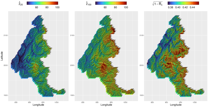
Figure 7: Comparison of the predicted angles and some extreme quantities. Top: Comparison with respect to the predicted GEV parameters $\mu$ (left), $\sigma$ (middle) and $\xi$ (right). Bottom: Comparison with respect to return levels of return period 20 years (left), 100 years (middle) and angular dispersion $V=\sqrt{1-\bar{R}_{n}}$ (right). For visualization purposes, angles have been dilated to put an emphasis on the snow season.

Since our model proposes a joint modeling of extremes and time of occurrence, it is possible to draw conclusion on their joint behavior. Figure 7 shows prediction maps of the days of occurrence, denoted by arrows, and the connection with extreme–related quantities (colored background). The top row investigates the relationship between time of occurrence and the GEV parameters. First, it seems that time of occurrence are not related to the scale and shape parameters. However and more interestingly, small values of the GEV location parameter are associated to earlier time of occurrence in the winter season and low elevation regions while large values yield to time of occurrences later in the winter season within high elevation regions. Because the GEV scale and shape parameters have little variations over the study region, the GEV quantiles are mainly driven by the location parameter and the above behavior is propagated to quantiles as illustrated by the first two maps of the bottom row of Figure 7. Consequently it seems that greater extremes seems to appear later in the season, i.e., in mid February, while moderate extremes are expected to happened in early January. Finally, the last map of Figure 7 indicates that a later expected time of occurrences is associated with a greater angular dispersion and greater dispersion coincides with high elevation. Although this result may have been anticipated since higher elevation increases the chance that rain turns into snowfall and, as consequence, yields to record snowfall occurring in a wider temporal window, it does not explain why the most severe events may occur later in the snowfall season.

7 Conclusion

Although the modeling of spatial extremes has made major development over the last decade, little attention has been put on the modeling of an angular related quantity associated with those extremes events, e.g., wind gust and wind direction. In this paper we proposed a Bayesian hierarchical model that enables the joint modeling of extremes events and an angular component. An inferential framework, based on MCMC algorithm, was proposed and applied on both a simulation study and an application on extreme snowfalls in the French Alps. Results show interesting results between magnitude of extremes and time of occurrence as well as dependence on some additional covariates such as elevation. Prediction maps are also available from our model. Our analysis opens some interesting questions though such as investigating the potential effect of climate change on time of occurrence or the duration of the winter season.

From a methodological point of view, the proposed model could serve as a basis for other approaches. More precisely, our approach relies on a conditional independence assumption which is not suited for modeling areal quantities such as the maximum snowfall in a sub–region (Davison et al.,, 2012). If areal quantities are of interest, one possible approach would be to rely on max-stable processes. However the use of max-stable process induces a theoretical challenge since the likelihood associated to these processes is extremely CPU demanding and one has to develop an elegant framework to overcome this computational burden.

Appendix: Gibbs sampler

Inference for our latent extreme–angular Bayesian hierarchical model may be performed using a Gibbs sampler, whose steps we now describe. To ease notations, we define $\boldsymbol{R}_{t}=\{R_{t}(s_{1}),\ldots,R_{t}(s_{k})\}$ and $\boldsymbol{\mu}_{t}=\{\mu_{t}(s_{1}),\ldots,\mu_{t}(s_{k})\}$ with similar for the GEV scale and shape parameters. Given a current value of the Markov chain

$$\psi_{t}=(\boldsymbol{R}_{t},\boldsymbol{\mu}_{t},\boldsymbol{\sigma}_{t},\boldsymbol{\xi}_{t},\rho_{t},\tau_{\mu},\tau_{\theta,t},\tau_{\sigma,t},\tau_{\xi,t},\lambda_{\theta,t},\lambda_{\mu,t},\lambda_{\sigma,t},\lambda_{\xi,t},\boldsymbol{\beta}_{\theta,t},\boldsymbol{\beta}_{\mu,t},\boldsymbol{\beta}_{\sigma,t},\boldsymbol{\beta}_{\xi,t}),$$

the next state $\psi_{t+1}$ of the chain is obtained as follows.

Step 1: Updating the GEV parameters at each site
Each component of $\boldsymbol{\mu}=\{\mu(s_{1}),\ldots,\mu(s_{k})\}$ is updated singly according to the following scheme. Generate a proposal $\mu_{p}(s_{j})$ from a symmetric random walk and compute the acceptance probability

$$\alpha\{\mu(s_{j}),\mu_{p}(s_{j})\}=\min\left\{1,r_{1}\{\mu(s_{j}),\mu_{p}(s_{j})\}r_{2}\{\mu(s_{j}),\mu_{p}(s_{j})\}r_{3}\{\mu(s_{j}),\mu_{p}(s_{j})\}\right\},$$

with

$$r_{1}\{\mu(s_{j}),\mu_{p}(s_{j})\} =\frac{\pi\{\eta(s_{j})\mid\mu_{p}(s_{j}),\sigma(s_{j}),\xi(s_{j})\}}{\pi\{\eta(s_{j})\mid\mu(s_{j}),\sigma(s_{j}),\xi(s_{j})\}}$$

$$r_{2}\{\mu(s_{j}),\mu_{p}(s_{j})\} =\prod\limits_{i=1}^{n}\frac{\pi\{R_{i}(s_{j}),\theta_{i}(s_{j})\mid\mu_{p}(s_{j}),\sigma(s_{j}),\xi(s_{j}),\boldsymbol{\beta}_{\theta},\rho,\tau_{\theta,t}\}}{\pi\{R_{i}(s_{j}),\theta_{i}(s_{j})\mid\mu(s_{j}),\sigma(s_{j}),\xi(s_{j}),\boldsymbol{\beta}_{\theta},\rho,\tau_{\theta,t}\}}$$

$$r_{3}\{\mu(s_{j}),\mu_{p}(s_{j})\} =\frac{\pi(\boldsymbol{\mu}_{p}\mid\boldsymbol{\beta}_{\mu},\tau_{\mu},\lambda_{\mu})}{\pi(\boldsymbol{\mu}\mid\boldsymbol{\beta}_{\mu},\tau_{\mu},\lambda_{\mu})}$$

where $r_{1}$ is a ratio of GEV likelihoods, $r_{2}$ a ratio of projected Gaussian likelihoods and $r_{3}$ a ratio multivariate Normal likelihoods. With probability $\alpha\{\mu(s_{j}),\mu_{p}(s_{j})\}$, the $\mu(s_{j})$ component of $\boldsymbol{\psi}_{t+1}$ is set to $\mu_{p}(s_{j})$; otherwise it remains at $\mu(s_{j})$. The scale and shape parameters are updated similarly.

Due to possible components related to $\mu,\sigma$ or $\xi$, the design matrix $D_{\theta}$ (related to the regression parameter $\beta_{\theta}$) needs to be updates each time one of those parameters is changed.

Step 2: Updating the radius at each site and replicate
Each component of $\mathbf{R}_{i}=\{R_{i}(s_{1}),\ldots,R_{i}(s_{k})\}$, $i=1,\ldots,n$, is updated singly according to the following scheme. Generate a proposal $R_{p,i}(s_{j})$ from a log-normal distribution and compute the acceptance probability

$$\alpha\{R_{i}(s_{j}),R_{p,i}(s_{j})\}=\min\left\{1,\frac{\pi(\mathbf{R}_{p,i},\boldsymbol{\theta}_{i}\mid\boldsymbol{\mu},\boldsymbol{\sigma},\boldsymbol{\xi},\boldsymbol{\beta}_{\theta},\tau_{\theta,t},\rho,\lambda_{\theta})}{\pi(\mathbf{R}_{i},\boldsymbol{\theta}_{i}\mid\boldsymbol{\mu},\boldsymbol{\sigma},\boldsymbol{\xi},\boldsymbol{\beta}_{\theta},\tau_{\theta,t},\rho,\lambda_{\theta})}\right\},$$

i.e., a ratio of radial Gaussian likelihoods, i.e., based on (4). With probability $\alpha\{R_{i}(s_{j}),R_{p,i}(s_{j})\}$, the $R_{i}(s_{j})$ component of $\boldsymbol{\psi}_{t+1}$ is set to $R_{p,i}(s_{j})$; otherwise it remains at $R_{i}(s_{j})$.

Step 3: Updating the angle regression parameters
Due to the use of conjugate priors, $\boldsymbol{\beta}_{\theta}$ is drawn directly from a multivariate Normal distribution having covariance matrix and mean vector

$$\{(\Sigma_{\theta}^{*})^{-1}+nD_{\theta}^{T}\Sigma_{\theta}^{-1}D_{\theta}\}^{-1},\quad\{(\Sigma_{\theta}^{*})^{-1}+D_{\theta}^{T}\Sigma_{\theta}^{-1}D_{\theta}\}^{-1}\{(\Sigma_{\theta}^{*})^{-1}\mu_{\theta}^{*}+D_{\theta}^{T}\Sigma_{\theta}^{-1}\sum\limits_{i=1}^{n}\mathbf{X}_{i}\}$$

where $\mu_{\theta}^{*}$ and $\Sigma_{\theta}^{*}$ are the mean vector and covariance matrix of the prior distribution for $\boldsymbol{\beta}_{\mu}$, $D_{\theta}$ is the design matrix related to the regression coefficients $\boldsymbol{\beta}_{\theta}$, $\mathbf{X}_{i}$ is the vector $\begin{pmatrix}\mathbf{R}_{i}\cos(\boldsymbol{\theta}_{i})&\mathbf{R}_{i}\sin(\boldsymbol{\theta}_{i})\end{pmatrix}^{\top}$ and $\Sigma_{\theta}$ the covariance matrix of $\mathbf{X}_{i}$.

Step 4: Updating the GEV regression parameters
Due to the use of conjugate priors, $\boldsymbol{\beta}_{\mu}$ is drawn directly from a multivariate Normal distribution having covariance matrix and mean vector

$$\{(\Sigma_{\mu}^{*})^{-1}+D_{\mu}^{T}\Sigma_{\mu}^{-1}D_{\mu}\}^{-1},\quad\{(\Sigma_{\mu}^{*})^{-1}+D_{\mu}^{T}\Sigma_{\mu}^{-1}D_{\mu}\}^{-1}\{(\Sigma_{\mu}^{*})^{-1}\mu_{\mu}^{*}+D_{\mu}^{T}\Sigma_{\mu}^{-1}\boldsymbol{\mu}\}$$

where $\mu_{\mu}^{*}$ and $\Sigma_{\mu}^{*}$ are the mean vector and covariance matrix of the prior distribution for $\boldsymbol{\beta}_{\mu}$, $D_{\mu}$ is the design matrix related to the regression coefficients $\boldsymbol{\beta}_{\mu}$ and $\Sigma_{\mu}$ the covariance matrix of $\boldsymbol{\mu}$. Again the regression parameters for the GEV scale and shape parameters are updated similarly.

Step 5: Updating the sill parameters of the covariance function
Due to the use of conjugate priors, $\tau_{\mu}$ is drawn directly from an inverse Gamma distribution whose shape and rate parameters are

$$\frac{k}{2}+\kappa_{\tau_{\mu}}^{*},\quad\theta_{\tau_{\mu}}^{*}+\frac{1}{2}\tau_{\mu}(\boldsymbol{\mu}-D_{\mu}\boldsymbol{\beta}_{\mu})^{T}\Sigma_{\mu}^{-1}(\boldsymbol{\mu}-D_{\mu}\beta_{\mu}),$$

where $\kappa_{\tau_{\mu}}^{*}$ and $\theta_{\tau_{\mu}}^{*}$ are respectively the shape and scale parameters of the inverse Gamma prior distribution. The sill parameters of the covariance function for the GEV scale and shape parameters are updated similarly.

Step 6: Updating the projected Gaussian parameters
To update the parameter $\tau_{\theta}$, we generate a proposal $\tau_{\theta,p}$ from a log-normal distribution and compute the acceptance probability

$$\alpha\{\tau_{\theta},\tau_{\theta,p}\}=\min\left\{1,\frac{\pi(\mathbf{R},\boldsymbol{\theta}\mid\boldsymbol{\mu},\boldsymbol{\sigma},\boldsymbol{\xi},\boldsymbol{\beta}_{\theta},\tau_{\theta,p},\rho,\lambda_{\theta})\pi(\tau_{\theta,p}\mid\kappa_{\tau_{\theta}}^{*},\theta_{\lambda_{\theta}}^{*})}{\pi(\mathbf{R},\boldsymbol{\theta}\mid\boldsymbol{\mu},\boldsymbol{\sigma},\boldsymbol{\xi},\boldsymbol{\beta}_{\theta},\tau_{\theta,t},\rho,\lambda_{\theta})\pi(\tau_{\theta,t}\mid\kappa_{\tau_{\theta}}^{*},\theta_{\lambda_{\theta}}^{*})}\frac{\tau_{\theta,p}}{\tau_{\theta}}\right\},$$

a ratio of projected Gaussian likelihood times the ratio of the prior densities with a correction due to the use of non symmetric proposal distribution and where $\kappa_{\tau_{\theta}}^{*}$ and $\theta_{\lambda_{\theta}}^{*}$ are respectively the shape and scale parameters of the Gamma prior distribution. With probability $\alpha\{\tau_{\theta},\tau_{\theta,p}\}$, the $\tau_{\theta}$ component of $\boldsymbol{\psi}_{t+1}$ is set to $\tau_{\theta,p}$; otherwise it remains at $\tau_{\theta,t}$. The parameter $\lambda$ is updated similarly as well as the parameter $\rho$ except that, for the latter parameter, we use the following symmetric proposal distribution $\rho_{p}\sim\rho+U(-\epsilon_{\rho},\epsilon_{\rho})$ and consequently no correction like $\rho_{p}/\rho$ is required.

Step 7: Updating the range parameters of the covariance function
To update the parameter $\lambda_{\mu}$, we generate a proposal $\lambda_{\mu,p}$ from a log-normal distribution and compute the acceptance probability

$$\alpha(\lambda_{\mu},\lambda_{\mu,p})=\min\left\{1,\frac{\pi(\boldsymbol{\mu}\mid\tau_{\mu},\lambda_{\mu,p},\boldsymbol{\beta}_{\mu})}{\pi(\boldsymbol{\mu}\mid\tau_{\mu},\lambda_{\mu},\boldsymbol{\beta}_{\mu})}\left(\frac{\lambda_{\mu,p}}{\lambda_{\mu}}\right)^{k_{\lambda_{\mu}}^{*}-1}\exp\left(\frac{\lambda_{\mu}-\lambda_{\mu,p}}{\theta_{\lambda_{\mu}}^{*}}\right)\frac{\lambda_{\mu,p}}{\lambda_{\mu}}\right\},$$

a ratio of multivariate Normal densities times the ratio of the prior densities and that of the proposal densities and where $\kappa_{\lambda_{\mu}}^{*}$ and $\theta_{\lambda_{\mu}}^{*}$ are respectively the shape and the scale parameters of the Gamma prior distribution. With probability $\alpha(\lambda_{\mu},\lambda_{\mu,p})$, the $\lambda_{\eta}$ component of $\boldsymbol{\psi}_{t+1}$ is set to $\lambda_{\mu,p}$; otherwise it remains at $\lambda_{\mu}$. The range parameters related to the scale and shape GEV parameters are updated similarly. If the covariance family has a shape parameter like the powered exponential or the Whittle–Matérn covariance functions, this is updated in the same way.

References

- Cooley et al., (2007) Cooley, D., Nychka, D., and Naveau, P. (2007). Bayesian spatial modeling of extreme precipitation return levels. J. Am. Stat. Assoc., 102(479):824–840.
- Cox, (1975) Cox, D. (1975). Discussion of professor mardia’s paper. Journal of the Royal Statistical Society: Series B (Methodological), 37:371–393.
- Davison et al., (2013) Davison, A., Huser, R., and Thibaud, E. (2013). Geostatistics of dependent and asymptotically independent extremes. Mathematical Geosciences, 45(5):511–529.
- Davison et al., (2012) Davison, A., Padoan, S., and Ribatet, M. (2012). Statistical modelling of spatial extremes. Statistical Science, 7(2):161–186.
- Davison and Gholamrezaee, (2011) Davison, A. C. and Gholamrezaee, M. M. (2011). Geostatistics of extremes. Proceedings of the Royal Society A: Mathematical, Physical and Engineering Science.
- de Haan and Fereira, (2006) de Haan, L. and Fereira, A. (2006). Extreme value theory: An introduction. Springer Series in Operations Research and Financial Engineering.
- Dombry et al., (2016) Dombry, C., Engelke, S., and Oesting, M. (2016). Exact simulation of max-stable processes. Biometrika, 103(2):303–317.
- Dombry et al., (2017) Dombry, C., Engelke, S., and Oesting, M. (2017). Bayesian inference for multivariate extreme value distributions. Electronic Journal of Statistics, 11(2):4813 – 4844.
- Dombry et al., (2013) Dombry, C., Éyi-Minko, F., and Ribatet, M. (2013). Conditional simulations of max-stable processes. Biometrika, 100(1):111–124.
- Durand et al., (2009) Durand, Y., Giraud, G., Laternser, M., Etchevers, P., Mérindol, L., and Lesaffre, B. (2009). Reanalysis of 47 years of climate in the french alps (1958–2005): Climatology and trends for snow cover. Journal of Applied Meteorology and Climatology, 48(12):2487 – 2512.
- Gelfand and Wang, (2013) Gelfand, A. and Wang, A. (2013). Directional data analysis under the general projected normal distribution. Statistical Methodology, pages 113–127.
- Gelfand and Wang, (2014) Gelfand, A. and Wang, A. (2014). Modeling space and space-time directional data using projected gaussian processes. Journal of the American Statistical Association.
- Gneiting and Raftery, (2007) Gneiting, T. and Raftery, A. E. (2007). Strictly proper scoring rules, prediction, and estimation. Journal of the American Statistical Association, 102(477):359–378.
- Grimit et al., (2006) Grimit, E. P., Gneiting, T., Berrocal, V. J., and Johnson, N. A. (2006). The continuous ranked probability score for circular variables and its application to mesoscale forecast ensemble verification. Quarterly Journal of the Royal Meteorological Society, 132(621C):2925–2942.
- Huser et al., (2019) Huser, R., Dombry, C., Ribatet, M., and Genton, M. (2019). Full–likelihood inference for max-stable processes. Stat, 8(1):e218.
- Huser and Genton, (2016) Huser, R. and Genton, M. G. (2016). Non-stationary dependence structures for spatial extremes. Journal of Agricultural, Biological, and Environmental Statistics, 21(3):470–491.
- Mardia, (1972) Mardia, K. (1972). Statistics of Directional Data. Academix Press.
- Mardia and Jupp, (2009) Mardia, K. and Jupp, P. (2009). Directional statistics. John Wiley and Sons.
- Mardia and Spurr, (1973) Mardia, K. V. and Spurr, B. D. (1973). Multisample tests for multimodal and axial circular populations. Journal of the royal statistical society series b-methodological, 35:422–436.
- Oesting et al., (2012) Oesting, M., Kabluchko, Z., and Schlather, M. (2012). Simulation of Brown–Resnick processes. Extremes, 15:89–107. 10.1007/s10687-011-0128-8.
- Padoan et al., (2010) Padoan, S., Ribatet, M., and Sisson, S. (2010). Likelihood-based inference for max-stable processes. Journal of the American Statistical Association (Theory & Methods), 105(489):263–277.
- Ribatet et al., (2012) Ribatet, M., Cooley, D., and Davison, A. (2012). Bayesian inference from composite likelihoods, with an application to spatial extremes. Statistica Sinica, 22:813–845.
- Richards and Wadsworth, (2021) Richards, J. and Wadsworth, J. (2021). Spatial deformation for non-stationary extremal dependence. Environmetrics, 32(5).
- Schlather, (2002) Schlather, M. (2002). Models for stationary max-stable random fields. Extremes, 5(1):33–44.
- Spiegelhalter et al., (2002) Spiegelhalter, D. J., Best, N. G., Carlin, B. P., and Van Der Linde, A. (2002). Bayesian measures of model complexity and fit. Journal of the Royal Statistical Society: Series B (Statistical Methodology), 64(4):583–639.
- Zhang, (2004) Zhang, H. (2004). Inconsistent estimation and asymptotically equal interpolations in model-based geostatistics. Journal of the American Statistical Association, 99(465):250–261.