Optimal control of port-Hamiltonian systems: energy, entropy, and exergy^∗

Abstract.

We consider irreversible and coupled reversible-irreversible nonlinear port-Hamiltonian systems and the respective sets of thermodynamic equilibria. In particular, we are concerned with optimal state transitions and output stabilization on finite-time horizons. We analyze a class of optimal control problems, where the performance functional can be interpreted as a linear combination of energy supply, entropy generation, or exergy supply. Our results establish the integral turnpike property towards the set of thermodynamic equilibria providing a rigorous connection of optimal system trajectories to optimal steady states. Throughout the paper, we illustrate our findings by means of two examples: a network of heat exchangers and a gas-piston system.

Keywords. energy, entropy, exergy, port-Hamiltonian systems, optimal control, turnpike property, thermodynamics, dissipativitiy, passivity

1. Introduction

Port-Hamiltonian systems provide a highly structured framework for energy-based modeling, analysis, and control of dynamical systems [6, 37]. A particular feature of port-Hamiltonian systems is that solutions satisfy an energy balance and the supplied energy is given as a product of the input and the colocated output. This motivates and enables the formulation and in-depth analysis of optimal control problems, e.g., output stabilization or state transition, in which the supplied energy is minimized: Whereas the choice of this cost functional is physically meaningful, it leads to singular optimal control problems. However, for linear port-Hamiltonian systems, the port-Hamiltonian structure can be exploited to establish regularity of the optimality system [11] (potentially after adding a rank-minimal regularization term) and to analyze the asymptotics of optimal solutions w.r.t. the conservative subspace [34, 13]. These results have been extended to infinite-dimensional linear systems  [25] and nonlinear reversible port-Hamiltonian systems  [21]. However, when the thermodynamic properties of the control systems have to be taken into account, other corresponding potentials than the free energy such as the internal energy and the entropy, have to be considered. In turn, the dynamics have to reflect both—the energy conservation and the entropy creation due to the irreversible phenomena.

The Hamiltonian formulation of controlled thermodynamic systems is an active field of research with various classes of systems ranging from dissipative Hamiltonian (or metriplectic) systems  [24, 18, 19] for the so-called GENERIC framework, irreversible port-Hamiltonian systems [30], to port-Hamiltonian systems defined on contact manifolds [7, 15, 14], and symplectic manifolds [38]. Different control design methods have been developed for these systems: stabilization based on control of either thermodynamic potentials such as the availability function [1, 2, 33, 39] or the entropy creation [17, 16], shaping of the entropy creation for irreversible port-Hamiltonian systems [28], and structure-preserving stabilizing feedback of contact Hamiltonian systems [29, 32].

In this work, we are concerned with optimal control of coupled reversible-irreversible port-Hamiltonian systems based on first preliminary steps conducted in our conference paper [23].

In view of applications, due to the strong nonlinearity, only stationary optimal control problems were considered for high-dimensional thermodynamic systems (arising, e.g., from discretizations of partial differential equations), see, e.g., [20, 5]. In [40, Section 13.5.2], the authors discuss highways in state space as particular sets, in which (or close to which) entropy optimal solutions reside. For non-stationary problems, such a behavior is coined the turnpike property [35, 10, 4].

The main contribution of this work is the proof of the turnpike property for optimal control of reversible-irreversible port-Hamiltonian systems. To this end, we formulate the dynamic problem of energy, entropy, and exergy optimization. We show that, for long time horizons, optimal solution trajectories of this problem stay close to the set of thermodynamic equilibria for the majority of the time. The corresponding result is proven for output stabilization and for state-transition problems. We further analyze the underlying steady-state problem in detail and we provide several numerical examples including a network of heat exchangers and a gas-piston system.

This paper is structured as follows: In Section 2, we recall the definition of the class of reversible-irreversible port-Hamiltonian systems and show that two examples embed into this framework: a heat exchanger and a gas-piston system. We provide conditions in terms of the Hamiltonian energy, which ensure that the set of thermodynamic equlibria is a manifold and characterize its dimension. Next, in Section 3, we consider and analyze the problem of optimal state transition, where optimality is understood as minimal energy supply, minimal entropy creation, or a combination of both as the exergy. In Section 4, we derive similar results for optimal output stabilization instead of state transition, demonstrating the generality of the developed tools. Finally, we illustrate our findings by reconsidering the two examples in numerical illustrations in Section 5 before conclusions are drawn in Section 6.

Notation. We denote the gradient of a scalar valued function $F:\mathbb{R}^{n}\to\mathbb{R}$ by $F_{x}$ and its Hessian by $F_{xx}$. The Poisson bracket with respect to a skew-symmetric matrix $J\in\mathbb{R}^{n\times n}$ of the differentiable functions $v,w:\mathbb{R}^{n}\to\mathbb{R}$ is defined by

$$\{v,w\}_{J}(x):=v_{x}(x)^{\top}Jw_{x}(x),\quad x\in\mathbb{R}^{n}.$$

Let $K\subset\mathbb{R}^{n}$. We write “$\alpha(x)\lesssim\beta(x)$ for $x\in K$” if there exists $c>0$ such that $\alpha(x)\leq c\beta(x)$ for $x\in K$. In addition, we write “$\alpha(x)\asymp\beta(x)$ for $x\in K$” if $\alpha(x)\lesssim\beta(x)$ and $\beta(x)\lesssim\alpha(x)$ for $x\in K$.

2. Coupled reversible-irreversible pH-Systems

In this section we provide the system class we analyze and illustrate it by means of two examples.

2.1. Definition of reversible-irreversible pH-Systems

The state space will be given by an open set $\mathbb{X}\subset\mathbb{R}^{n}$, $n\in\mathbb{N}$. As usual in finite-dimensional pH systems, input and output space coincide; here, inputs and outputs are elements of $\mathbb{R}^{m}$, $m\in\mathbb{N}$. The following definition of coupled reversible-irreversible pH Systems was given in [31].

Definition 2.1 (Reversible-irreversible pH-Systems).

A Reversible-Irreversible port-Hamiltonian system (RIPHS) is defined by

• a locally Lipschitz-continuous map $J_{0}:\mathbb{X}\to\mathbb{R}^{n\times n}$ of skew-symmetric Poisson structure matrices $J_{0}(x)$, $x\in\mathbb{X}$,

• a differentiable Hamiltonian function $H:\mathbb{X}\to\mathbb{R}$, whose gradient $H_{x}:\mathbb{X}\to\mathbb{R}^{n}$ is locally Lipschitz-continuous,

• a differentiable entropy function $S:\mathbb{X}\to\mathbb{R}$, whose gradient $S_{x}:\mathbb{X}\to\mathbb{R}^{n}$ is locally Lipschitz-continuous and which is a Casimir function of the Poisson structure matrix function $J_{0}$, that is, $J_{0}(x)S_{x}(x)=0$ for all $x\in\mathbb{X}$,

• $N$ constant skew-symmetric structure matrices $J_{k}\in\mathbb{R}^{n\times n}$, $k=1,\ldots,N$,

• functions $\gamma_{1},\ldots,\gamma_{N}:\mathbb{R}^{2n}\to\mathbb{R}$ such that $\gamma_{k}\left(\,\cdot\,,H_{x}(\cdot)\right):\mathbb{X}\to\mathbb{R}$ is positive and locally Lipschitz-continuous for all $k=1,\ldots,N$,

• a locally Lipschitz-continuous input matrix function $g:\mathbb{R}^{2n}\to\mathbb{R}^{n\times m}$,

the state equation

$$\dot{x}=\Big{(}J_{0}(x)+\sum_{k=1}^{N}\gamma_{k}(x,H_{x})\left\{S,H\right\}_{J_{k}}J_{k}\Big{)}H_{x}(x)+g(x,H_{x})u,$$ (RIPHS)

and two conjugate outputs, corresponding to the energy and the entropy, respectively, defined by

$$y_{H}:=g(x,H_{x})^{\top}H_{x}\qquad\text{and}\qquad y_{S}:=g(x,H_{x})^{\top}S_{x}.$$ (2.1)

If $J_{0}\equiv 0$ and $N=1$, the system is called an irreversible port-Hamiltonian system (IPHS).

By means of direct calculations, any trajectory $x\in C^{1}(0,T;\mathbb{X})$ satisfying the dynamics (RIPHS) can be shown to obey both the energy balance

$$\frac{\text{d}}{\text{d}t}H(x(t)) =y_{H}(t)^{\top}u(t)$$ (2.2)

and the entropy balance

$$\frac{\text{d}}{\text{d}t}S(x_{t}) =\sum_{k=1}^{N}\gamma_{k}\big{(}x_{t},H_{x}(x_{t})\big{)}\{S,H\}_{J_{k}}^{2}(x_{t})+y_{S}(t)^{\top}u(t)$$ (2.3)

where $x_{t}=x(t)$. Here, the quantity $y_{H}^{\top}u$ in (2.2) represents the energy flow, i.e., the power supplied to the system, whereas $y_{S}^{\top}u$ in (2.3) stands for the entropy flow injected into the system. The positivity of the sum on the right-hand side of the entropy balance captures the irreversible nature of the particular phenomenon. For closed systems, i.e., where $g(x,H_{x})\equiv 0$, it can be directly read off these equations that energy is preserved and entropy is non-decreasing, hence the two fundamental laws of thermodynamics are satisfied.

For $u=0$, a thermodynamic equilibrium is attained if the first term on the right-hand side of (2.3) vanishes. The set of thermodynamic equilibria

$$\mathcal{T}:= \Big{\{}x\in\mathbb{X}:\sum_{k=1}^{N}\gamma_{k}(x,H_{x}(x))\{S,H\}^{2}_{J_{k}}(x)=0\Big{\}}$$

$$= \big{\{}x\in\mathbb{X}:\{S,H\}_{J_{k}}(x)=0\,\,\text{for all }k=1,\ldots,N\big{\}},$$

plays a distinguished role in this paper. In the set definition above the second equality follows from positivity of $\gamma$. Notice that, at first glance the power balance (2.2) suggests that the system does not dissipate energy. However, in reversible-irreversible systems, dissipation corresponds to an increase of temperature and thus it implies entropy growth. In particular, any port-Hamiltonian system with linear dissipation may be written as an RIPHS by adding a virtual heat compartment.

Remark 2.2 (Linear and affine input structures).

Note that the input map in Definition 2.1 is linear in the input, contrary to the setting in [31] where it is affine. This choice corresponds to a reversible interconnection of the system with its environment as discussed in [22].

Remark 2.3 (Local existence of solutions).

Given $u\in L^{\infty}_{\rm loc}(t_{0},t_{f})$, the local Lipschitz conditions on the functions $J_{0}$, $H_{x}$, $S_{x}$, $\gamma_{k}$, and $g$ guarantee at least local existence and uniqueness of solutions of initial value problems with dynamics (RIPHS).

In the next lemma, we assume that the entropy $S$ is linear in the state $x$. This is not a restrictive assumption as in many physical examples, where the Hamiltonian $H$ contains the internal energies of subsystems, the total entropy is simply the sum of some coordinates of the state (see Example 2.7 below).

Lemma 2.4.

The set of thermodynamic equilibria $\mathcal{T}$ is closed in $\mathbb{X}$. If $S(x)=e^{\top}x$ with some $e\in\mathbb{R}^{n}$ and for all $x\in\mathbb{X}$, we have

$$\operatorname{rank}\left[\begin{smallmatrix}H_{xx}(x)\\ H_{x}(x)^{\top}\end{smallmatrix}\right]=n,$$ (2.4)

then $\mathcal{T}$ is a $C^{1}$-submanifold of $\mathbb{X}$. It is empty if and only if $H_{x}(\mathbb{X})\cap\bigcap_{k=1}^{N}(J_{k}e)^{\perp}=\varnothing$. Otherwise, its dimension is given by

$$\dim\mathcal{T}=n-\operatorname{rank}[J_{1}e\cdots J_{N}e].$$

Proof.

As the Poisson bracket $\{S,H\}_{J_{k}}$ is continuous for any $k\in\{1,\ldots,N\}$, it is clear that $\mathcal{T}$ is closed in $\mathbb{X}$. Now, assume that $S(x)=e^{\top}x$ and that (2.4) holds. Set $v_{k}=J_{k}e$, $k=1,\ldots,N$. Note that

$$\{S,H\}_{J_{k}}=S_{x}^{\top}J_{k}H_{x}=e^{\top}J_{k}H_{x}=-v_{k}^{\top}H_{x}.$$

If $v_{1}=\ldots=v_{N}=0$, then $\mathcal{T}=H_{x}^{-1}(\mathbb{R}^{n})=\mathbb{X}$ and thus $\dim\mathcal{T}=n$, as claimed. Otherwise, $r:=\operatorname{rank}[v_{1}\dots v_{n}]\geq 1$. We assume without loss of generality that $v_{1},\ldots,v_{r}$ are linearly independent and define $f:\mathbb{X}\to\mathbb{R}^{r}$ by

$$f(x)=[v_{1},\dots,v_{r}]^{\top}H_{x}(x).$$

Note that $\mathcal{T}=f^{-1}(\{0\})$. We have $Df(x)=[v_{1},\dots,v_{r}]^{\top}H_{xx}(x)$, $x\in\mathbb{X}$. Let $x_{0}\in\mathcal{T}$, i.e., $H_{x}(x_{0})^{\top}v_{k}=0$ for $k=1,\ldots,r$ and suppose that $Df(x_{0})$ is not surjective, i.e., there exists some $w\in\mathbb{R}^{r}\backslash\{0\}$ such that $H_{xx}(x_{0})[v_{1},\dots v_{r}]w=0$. Consequently,

$$\left[\begin{smallmatrix}H_{xx}(x)\\ H_{x}(x)^{\top}\end{smallmatrix}\right][v_{1},\dots v_{r}]w=0,$$

so that, by assumption, $[v_{1},\dots v_{r}]w=0$. But $v_{1},\dots,v_{r}$ are linearly independent so that $w=0$, a contradiction. Therefore, zero is a regular value of the $C^{1}$-function $f$, hence $\mathcal{T}=f^{-1}(\{0\})$ is a $C^{1}$-submanifold of $\mathbb{X}$ of the given dimension, cf. [41, Theorem 73C, p. 556]. ∎

We close this introductory subsection with the observation that the class of reversible-irreversible port-Hamiltonian systems is invariant under linear coordinate transforms. The proof follows by straightforwad computations and hence is omitted.

Proposition 2.5.

If $x$ solves (RIPHS) and $V\in\mathbb{R}^{n\times n}$ is invertible, then $z=Vx$ solves the reversible-irreversible pH-system

$$\dot{z}=\Big{(}\widetilde{J}_{0}(z)+\sum_{k=1}^{N}\widetilde{\gamma}_{k}(z,\widetilde{H}_{z})\big{\{}\widetilde{S},\widetilde{H}\big{\}}_{\widetilde{J}_{k}}\widetilde{J}_{k}\Big{)}\widetilde{H}_{z}(z)+\tilde{g}(z,\widetilde{H}_{z})u$$

with energy Hamiltonian $\widetilde{H}(z)=H(x)$, entropy $\widetilde{S}(z)=S(x)$,

$$\widetilde{J}_{0}(z)=VJ_{0}(x)V^{\top},\quad\widetilde{J}_{k}=VJ_{k}V^{\top},$$

and

$$\widetilde{g}(z,\widetilde{H}_{z})=Vg(V^{-1}z,V^{\top}\widetilde{H}_{z}),\quad\widetilde{\gamma}_{k}(z,\widetilde{H}_{z})=\gamma_{k}(V^{-1}z,V^{\top}\widetilde{H}_{z}).$$

2.2. Tutorial Examples

Next, we illustrate the class of (RIPHS) systems with two examples from thermodynamics: a heat exchanger and a gas-piston system.

Example 2.6 (Heat exchanger).

Let us consider a very simple model of a heat exchanger as depicted in Figure 1. The example is slightly adapted from [27]. The variables $T_{i}$,$S_{i}$, and $H_{i}$ denote the temperature, the entropy and the energy in compartment $i=1,2$, respectively.

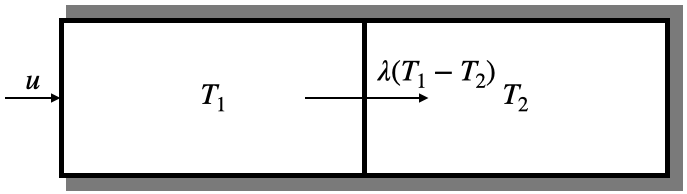
Figure 1. Simple model of a heat exchanger

Assuming that the walls are non-deformable and impermeable, the thermodynamic properties of each compartment are given by the following relation between the temperature and the entropy

$$T_{i}(S_{i})=T_{\text{ref}}\cdot e^{(S_{i}-S_{\text{ref}})/c_{i}},\qquad i=1,2,$$ (2.5)

where $S_{\text{ref}}\in\mathbb{R}$ is a reference entropy corresponding to the reference temperature $T_{\text{ref}}$ and $c_{i}$, $i=1,2$, are heat capacities, cf. [3, Section 2.2]. The energy in each compartment, denoted by $H_{i}(S_{i})$, $i=1,2$, can be obtained by integrating Gibbs’ equation $\text{d}H_{i}=T_{i}\text{d}S_{i}$ as a primitive of the function $T_{i}(S_{i})$, $i=1,2$. The state of our IPHS is $x=\begin{bmatrix}S_{1}&S_{2}\end{bmatrix}^{\top}$ and the total energy (entropy) is given by the sum of the energies (entropies, resp.) in the compartments, i.e.,

$$H(x)=H_{1}(S_{1})+H_{2}(S_{2})\quad\text{and}\quad S(x)=S_{1}+S_{2}=\begin{bmatrix}1&1\end{bmatrix}x.$$

We first assume that the outer walls are perfectly isolated, i.e., there is only heat flux through the conducting wall in between the two compartments given by Fourier’s law

$$q=\lambda(T_{1}-T_{2}).$$ (2.6)

On the other hand, the change in energy is given by the heat flux and thus, by continuity of the latter, we have

$$q=-\tfrac{\text{d}}{\text{d}t}H_{1}(S_{1}(t))=\tfrac{\text{d}}{\text{d}t}H_{2}(S_{2}(t)).$$

By Gibb’s equation we have $\frac{\mathrm{d}}{\mathrm{d}t}(H_{j}\circ S_{j})=\frac{\mathrm{d}H_{j}}{\mathrm{d}S_{j}}\cdot\frac{\mathrm{d}}{\mathrm{d}t}S_{j}=T_{j}\cdot\frac{\mathrm{d}}{\mathrm{d}t}S_{j}$. Hence,

$$\lambda(T_{1}-T_{2})=-T_{1}\tfrac{\text{d}}{\text{d}t}S_{1}(t)=T_{2}\tfrac{\text{d}}{\text{d}t}S_{2}(t).$$

Rearranging this equation yields the Hamiltonian-like formulation

$$\tfrac{\text{d}}{\text{d}t}\begin{bmatrix}S_{1}(t)\\ S_{2}(t)\end{bmatrix}=\lambda\big{(}\tfrac{1}{T_{2}(t)}-\tfrac{1}{T_{1}(t)}\big{)}\underbrace{\begin{bmatrix}0&-1\\ 1&0\end{bmatrix}}_{=:J}\begin{bmatrix}T_{1}(t)\\ T_{2}(t)\end{bmatrix}.$$

To complete the definition of an uncontrolled IPHS, we set

$$\gamma(x,H_{x})=\tfrac{\lambda}{T_{1}T_{2}}.$$

Then, as

$$\qquad\{S,H\}_{J}=\big{[}1\quad 1\big{]}\,J\begin{bmatrix}T_{1}\\ T_{2}\end{bmatrix}=T_{1}-T_{2},$$

the above ODE is of the form (RIPHS) with $J_{0}\equiv 0$, $N=1$, and $g(x,H_{x})\equiv 0$.

Entropy flow control. The first possible choice of an input would be to control the entropy flow $u$ into or out of compartment one, cf. Figure 1, cf. [27, Section 4.4.4]. In this case, we have $g(x,H_{x})\equiv\left[\begin{smallmatrix}1\\ 0\end{smallmatrix}\right]$ and hence the dynamics

$$\frac{\text{d}}{\text{d}t}\begin{bmatrix}S_{1}\\ S_{2}\end{bmatrix} =\gamma(x,H_{x})\{S,H\}_{J}(x)JH_{x}+\begin{bmatrix}1\\ 0\end{bmatrix}u.$$ (2.7)

Control by thermostat. A choice which is realizable in practise is to connect the first compartment to a thermostat with a controlled temperature $T_{e}$. Consequently, the heat flow between this compartment and the thermostat can be described via

$$q_{e}=\lambda_{e}(T_{e}-T_{1}),$$

with $\lambda_{e}>0$ being a heat conduction coefficient.

In this case, the entropy flow control (2.7) is related to the thermostat temperature control $T_{e}$ by the state dependent control transformation

$$u=\tfrac{T_{e}-T_{1}}{T_{1}}$$ (2.8)

Example 2.7 (Gas-piston system, cf. [36, 31]).

Let us briefly recall the model of a gas contained in a cylinder closed by a piston subject to gravity. Contrary to the previous example of the heat exchanger which was purely thermodynamic, the gas-piston system will encompass the thermodynamic and the mechanical domain.

Energy and co-energy variables. Consider the gas in the cylinder under the piston and assume that it is closed, i.e., there is no leakage. Then, the internal energy $U$ of the gas may be expressed as a function of its entropy $S$ and its volume $V$. For an ideal gas (see [7]), we have

$$U(S,V)=\frac{3}{2}\,NRT_{0}\cdot e^{\beta(S,V)},$$ (2.9)

with the ideal gas constant $R$ and

$$\beta(S,V)=\frac{S-Ns_{0}+RN{\rm ln}(NRT_{0})-RN{\rm ln}(VP_{0})}{\frac{3}{2}RN}$$ (2.10)

where $s_{0},\,T_{0},P_{0}$ are positive reference values.

Assume that the energy of the piston consists of the sum of the gravity potential energy and kinetic energy:

$$H_{mec}=\frac{1}{2m}\,p^{2}+mgz,$$

where $z$ denotes the altitude of the piston, $p$ its kinetic momentum, and $m$ its mass. If we assume that the gas fills all the volume below of the piston, then we have $Az=V$ where $A$ stands for the base area of the piston’s head. Hence one may choose the vector of state or energy variables $x=[S,V,p]^{\top}$ and the total energy of the system is given by

$$H(x)=U(S,V)+H_{mec}(V,p)$$

where

$$H_{mec}(V,p)=\frac{1}{2m}\,p^{2}+\frac{mg}{A}V.$$

The differential of the energy defines the co-energy variables

$$\frac{\partial H}{\partial S} =\frac{\partial U}{\partial S}=T_{0}\,e^{\beta(S,V)}=T(S,V)$$ (2.11a)

$$\frac{\partial H}{\partial V} =\frac{\partial U}{\partial V}+\frac{\partial H_{\rm mec}}{\partial V}=-P(S,V)+\frac{mg}{A}=\frac{-NRT_{0}\,e^{\beta(S,V)}}{V}+\frac{mg}{A}$$ (2.11b)

$$\frac{\partial H}{\partial p} =\frac{\partial H_{\text{mec}}}{\partial p}=\frac{p}{m}=v(p)$$ (2.11c)

where $T$ is the temperature, $P$ is the pressure, and $v$ is the velocity of the piston.

Dynamics: reversible and irreversible coupling. The model consists of three coupled balance equations. It may be written as a quasi-Hamiltonian system with a skew-symmetric structure matrix depending on two co-energy variables, the velocity $v$ and the temperature $T$:

$$\frac{d}{dt}\begin{bmatrix}S\\ V\\ p\end{bmatrix}=\underbrace{\begin{bmatrix}0&0&\frac{\kappa v}{T}\\ 0&0&A\\ -\frac{\kappa v}{T}&-A&0\end{bmatrix}}_{=:J_{irr}\left(T,v\right)}\underbrace{\begin{bmatrix}T\\ -P+\frac{mg}{A}\\ v\end{bmatrix}}_{H_{x}}.$$ (2.12)

The first equation is the entropy balance accounting for the irreversible creation of entropy associated with the non-reversible phenomena due to mechanical friction and viscosity of the gas when the piston moves. The second equation relates the variation of the volume of the gas to the velocity of the piston. The last equation is the momentum balance equation accounting for the mechanical forces induced by gravity, the pressure of the gas, and the total resistive forces which are assumed to be linear in the velocity of the piston, i.e., $F_{r}(v)=\kappa v$ with a scalar constant $\kappa\geq 0$.

The system (2.12) may be written in the form of (RIPHS) by decomposing further the structure matrix

$$J_{irr}\left(T,v\right)=J_{0}+R\left(x,H_{x},S_{x}\right)J_{1}$$

with the constant Poisson structure matrix associated with the reversible coupling

$$J_{0}=\begin{bmatrix}0&0&0\\ 0&0&A\\ 0&-A&0\end{bmatrix}$$

Since $S_{x}(x)=[1,0,0]^{\top}$, we have $J_{0}S_{x}=0$, i.e., the entropy is a Casimir function of $J_{0}$, as required in Definition 2.1(iii). The second structure matrix corresponding to the dissipative phenomenon, that is, the friction of the piston is given by

$$J_{1}=\begin{bmatrix}0&0&1\\ 0&0&0\\ -1&0&0\end{bmatrix}.$$

The modulating function for the irreversible phenomenon is

$$R(x,H_{x},S_{x})=\gamma(x,H_{x})\{S,H\}_{J_{1}},$$

which is composed by the the Poisson bracket

$$\{S,H\}_{J_{1}}=\begin{bmatrix}1&0&0\end{bmatrix}J_{1}\begin{bmatrix}T\\ -P\\ v\end{bmatrix}=v,$$

which is indeed the driving force inducing the mechanical friction and viscosity forces in the gas, and the positive function

$$\gamma\left(x,H_{x}\right)=\gamma\left(T\right)=\frac{\kappa}{T}.$$

Control input. For the purpose of illustration, we assume that the system is controlled by a heat flow $u$ entering the first line of the dynamics (2.12), similar to the entropy flow in (2.7). Similar to the heat exchanger it would be more realistic to assume that this heat flow is generated by a thermostat at controlled temperature $T_{e}$, interacting with the gas through a heat conducting wall leading to the same control transformation (2.8).

3. Optimal state transitions

Let a horizon $t_{f}\geq 0$, an initial state $x^{0}\in\mathbb{X}$ and a terminal region $\Phi\subset\mathbb{X}$ be given and assume that $\mathbb{U}\subset\mathbb{R}^{m}$ is compact and convex, containing the origin in its interior, i.e., $0\in\operatorname{int}\mathbb{U}$. Let $\alpha_{1},\alpha_{2}>0$ and consider the prototypical optimal control problem

$$\begin{split}\min_{u\in\mathcal{M}(0,t_{f};\mathbb{U})}\int_{0}^{t_{f}}&\left[\alpha_{1}y_{H}(t)-\alpha_{2}T_{0}y_{S}(t)\right]^{\top}u(t)\,\text{d}t\\ \text{s.t. }\eqref{eq:RIPHS},\quad&x(0)=x^{0},\quad x(t_{f})\in\Phi,\quad\eqref{eq:outputs},\end{split}$$ (phOCP)

where $T_{0}>0$ is a reference temperature and $\mathcal{M}(0,t_{f};\mathbb{U})$ denotes the space of all measurable functions $u:[0,t_{f}]\to\mathbb{U}$. From this optimal control problem, we can recover three important choices for the cost functional:

• $\alpha_{1}=1$, $\alpha_{2}=0$: Minimal energy supply.

• $\alpha_{1}=0$, $\alpha_{2}=1$: Minimal entropy extraction.

• $\alpha_{1}=1$, $\alpha_{2}=1$: Minimal exergy supply.

Setting $\ell_{\alpha_{1},\alpha_{2}}(x,u)=[\alpha_{1}y_{H}-\alpha_{2}T_{0}y_{S}]^{\top}u$ and using the balance equations (2.2) and (2.3), we obtain the identity

$$\begin{split}\int_{0}^{t_{f}}\ell_{\alpha_{1},\alpha_{2}}(x,u)\,\text{d}t&=\alpha_{1}\left[H(x(t_{f}))-H(x^{0})\right]\\ &\qquad+\alpha_{2}T_{0}\left(\!S(x^{0})-S(x(t_{f}))+\!\sum_{k=1}^{N}\int_{0}^{t_{f}}\!\!\!\gamma_{k}(x,H_{x})\{S,H\}^{2}_{J_{k}}\,\text{d}t\right).\end{split}$$ (3.1)

3.1. Optimal steady states

In this part, we analyze the steady-state counterpart of (phOCP). In the literature considering entropy optimization, in particular in the context of distributed parameter systems, the steady state problem is often considered due to the high complexity of the dynamic problem, cf. e.g. [20] for a plug flow reactor model and [5] for a binary tray distillation process.

In the turnpike result established in Subsection3.2, we provide a rigorous connection between dynamic and static problem, stating that entropy-, energy-, and entropy-optimal solutions for the dynamic problem are close to optimal solutions of the steady state for the majority of the time. This in particular consolidates the central role of the steady state problem in the context of (dynamic) optimal control for irreversible systems.

To simplify notation, we write

$$f(x,u)=\widetilde{J}(x)H_{x}(x)+g(x,H_{x})u,$$

where

$$\widetilde{J}(x)=J_{0}(x)+\sum_{k=1}^{N}\gamma_{k}(x,H_{x})\cdot\{S,H\}_{J_{k}}\!(x)\,J_{k}.$$ (3.2)

Then (RIPHS) reads $\dot{x}=f(x,u)$. A steady state of (RIPHS) is a pair $(\bar{x},\bar{u})\in\mathbb{X}\times\mathbb{U}$ for which $f(\bar{x},\bar{u})=0$. In particular, the constant trajectory $x(t)\equiv\bar{x}$ is a solution to $\dot{x}=f(x,\bar{u})$.

The steady state optimal control problem corresponding to (phOCP) reads as follows:

$$\min_{(\bar{x},\bar{u})\in\mathbb{X}\times\mathbb{U}}\ell_{\alpha_{1},\alpha_{2}}(\bar{x},\bar{u})\qquad\text{s.t.}\quad f(\bar{x},\bar{u})=0.$$ (3.3)

Any solution of this problem will be called an optimal steady state for (phOCP).

Proposition 3.1.

If $(\bar{x},\bar{u})$ is a steady state of (RIPHS), then

$$\ell_{\alpha_{1},\alpha_{2}}(\bar{x},\bar{u})=\alpha_{2}T_{0}\cdot\sum_{k=1}^{N}\gamma_{k}(\bar{x},H_{x}(\bar{x}))\cdot\{S,H\}_{J_{k}}^{2}(\bar{x})\geq 0.$$ (3.4)

In particular, the optimal value of (3.3) is always non-negative and it is zero if and only if the set

$$\mathcal{S}=\{(\bar{x},\bar{u})\in\mathcal{T}\times\mathbb{U}:g(\bar{x},H_{x}(\bar{x}))\bar{u}=-J_{0}(\bar{x})H_{x}(\bar{x})\}$$

is non-empty. In this case, the set $\mathcal{S}$ coincides with the set of optimal steady states for (phOCP). If $H_{x}(\hat{x})\in\operatorname{span}\{S_{x}(\hat{x})\}$ for some $\hat{x}\in\mathbb{X}$, we have $(\hat{x},0)\in\mathcal{S}$.

Proof.

Assuming $f(\bar{x},\bar{u})=0$, we compute

$$\ell_{\alpha_{1},\alpha_{2}}(\bar{x},\bar{u}) =\alpha_{1}\cdot y_{H}^{\top}\bar{u}-\alpha_{2}T_{0}\cdot y_{S}^{\top}\bar{u}$$

$$=\big{[}\alpha_{1}\cdot H_{x}(\bar{x})-\alpha_{2}T_{0}\cdot S_{x}(\bar{x})\big{]}^{\top}g(\bar{x},H_{x}(\bar{x}))\bar{u}$$

$$=-\big{[}\alpha_{1}\cdot H_{x}(\bar{x})-\alpha_{2}T_{0}\cdot S_{x}(\bar{x})\big{]}^{\top}\widetilde{J}(\bar{x})H_{x}(\bar{x})$$

$$=\alpha_{2}T_{0}\cdot S_{x}(\bar{x})^{\top}\widetilde{J}(\bar{x})H_{x}(\bar{x}).$$

Now, we substitute $\widetilde{J}(\bar{x})$ with the right hand side from (3.2), further we note that $S_{x}(\bar{x})^{\top}J_{0}(\bar{x})=0$ (see Definition 2.1 (iii)) and obtain (3.4).

Let $(\hat{x},\hat{u})\in\mathcal{S}$. Then $J_{0}(\hat{x})H_{x}(\hat{x})+g(\hat{x},H_{x}(\hat{x}))\hat{u}=0$, and, as $\hat{x}\in\mathcal{T}$, we also have $\{S,H\}_{J_{k}}(\hat{x})=0$ for all $k=1\ldots,N$. Hence $f(\hat{x},\hat{u})=0$, which means that $(\hat{x},\hat{u})$ is a steady state of (RIPHS). The first part of the proposition hence further implies that $\ell_{\alpha_{1},\alpha_{2}}(\hat{x},\hat{u})=0$, which shows that the optimal value of (3.3) is indeed zero and that $(\hat{x},\hat{u})$ is an optimal steady state for (phOCP). If $(\bar{x},\bar{u})$ is any other optimal steady state for (phOCP), then (3.4) implies that also $\{S,H\}_{J_{k}}\!(\bar{x})=0$ for $k=1,\ldots,N$. That is, $(\bar{x},\bar{u})\in\mathcal{S}$.

If the optimal value of (3.3) is zero and $(\bar{x},\bar{u})$ is a minimizer, then (3.4) implies that $\bar{x}\in\mathcal{T}$ and thus $(\bar{x},\bar{u})\in\mathcal{S}$.

Now suppose that there exists some $\hat{x}\in\mathbb{R}^{n}$ such that $H_{x}(\hat{x})\in\operatorname{span}\{S_{x}(\hat{x})\}$. Let $H_{x}(\hat{x})=\kappa\cdot S_{x}(\hat{x})$ for some $\alpha\in\mathbb{R}$. Then we have $\{S,H\}_{J_{k}}(\hat{x})=S_{x}(\hat{x})^{\top}J_{k}H_{x}(\hat{x})=0$ for all $k=1,\ldots,N$, thus $\hat{x}\in\mathcal{T}$. Moreover, $J_{0}(\hat{x})H_{x}(\hat{x})=0$ by Definition 2.1 (iii). This implies $(\hat{x},0)\in\mathcal{S}$. ∎

Corollary 3.2.

In the irreversible case, i.e., $J_{0}\equiv 0$ and $N=1$, we have $\mathcal{T}\times\{0\}\subset\mathcal{S}$. In particular, if $\mathcal{T}$ is non-empty, then so is $\mathcal{S}$ and thus $\mathcal{S}$ coincides with the set of all optimal steady states for (phOCP).

Having defined the sets $\mathcal{T}$ of thermodynamic equilibria, and the set $\mathcal{S}$ being closely related to optimal steady states, a third set comes into play, which is the set of thermodynamic equilibria which can be losslessly maintained while obeying the dynamics of (RIPHS):

$$\mathcal{T}_{\rm opt}:=\{\bar{x}\in\mathcal{T}:\exists\bar{u}\in\mathbb{U}\text{ with }(\bar{x},\bar{u})\in\mathcal{S}\}.$$

Note that in the irreversible case we have $\mathcal{T}_{\rm opt}=\mathcal{T}$.

3.2. Turnpikes towards thermodynamic equilibria

In this subsection we shall impose the following assumptions on the Hamiltonian $H$ and the entropy function $S$.

Assumption 3.3.

foo

1. $H\in C^{2}(\mathbb{X},\mathbb{R})$, the image $\mathbb{Y}:=H_{x}(\mathbb{X})$ is open in $\mathbb{R}^{n}$, and $H_{x}:\mathbb{X}\to\mathbb{Y}$ is a diffeomorphism.

2. $S(x)=e^{\top}x$ with some $e\in\mathbb{R}^{n}\backslash\{0\}$, i.e., the entropy is linear in the state.

Note that Lemma 2.4 implies that under these assumptions the set of thermodynamic equilibria $\mathcal{T}$ is a $C^{1}$-submanifold of $\mathbb{R}^{n}$.

We briefly verify Assumption 3.3 for the two examples of the previous section.

Example 3.4.

(a) We consider the heat exchanger from Example 2.6. Here, the state space is $\mathbb{X}=\mathbb{R}^{2}$. The entropy $S$ is given by $S(x)=e^{\top}x$, where $e=\begin{bmatrix}1&1\end{bmatrix}^{\top}$, and the Hamiltonian $H$ is a $C^{2}$-function with

$$H_{x}(S_{1},S_{2})=T_{\rm ref}\begin{bmatrix}e^{(S_{1}-S_{\rm ref})/c_{1}}\\ e^{(S_{2}-S_{\rm ref})/c_{2}}\end{bmatrix}.$$

Hence, $\mathbb{Y}=(0,\infty)\times(0,\infty)$, and $H_{x}:\mathbb{X}\to\mathbb{Y}$ is bijective with the continuously differentiable inverse function $H_{x}^{-1}:\mathbb{Y}\to\mathbb{X}$,

$$H_{x}^{-1}(T_{1},T_{2})=S_{\rm ref}\begin{bmatrix}1\\ 1\end{bmatrix}-(\ln T_{\rm ref})\begin{bmatrix}c_{1}\\ c_{2}\end{bmatrix}+\begin{bmatrix}c_{1}\ln T_{1}\\ c_{2}\ln T_{2}\end{bmatrix}.$$

(b) In case of the gas-piston system (Example 2.7), the entropy is a part of the state: $S(x)=\begin{bmatrix}1&0&0\end{bmatrix}x$. Concerning the energy variables $S$, $V$, and $p$, we allow $S$ and $p$ to assume any real value and $V$ only assumes values in an interval $(0,V_{\max})$, $V_{\max}>0$. The state space is thus given by $\mathbb{X}=\mathbb{R}\times(0,V_{\max})\times\mathbb{R}$. The image of $H_{x}$ then equals

$$\mathbb{Y}=\left\{\begin{bmatrix}T\\ -P+\frac{mg}{A}\end{bmatrix}:T>0,\;P>\frac{RNT}{V_{\max}}\right\}\times\mathbb{R}.$$

This easily follows from the representation

$$C_{0}\cdot e^{\frac{2S}{3RN}}\begin{bmatrix}(P_{0}V)^{-2/3}\\ -RNP_{0}(P_{0}V)^{-5/3}\end{bmatrix}+\begin{bmatrix}0\\ \frac{mg}{A}\end{bmatrix}$$

of the first two components of $H_{x}(S,V,p)$, where

$$C_{0}=T_{0}^{5/3}(RN)^{2/3}e^{-\frac{2s_{0}}{3R}}.$$

The inverse map $H_{x}^{-1}:\mathbb{Y}\to\mathbb{X}$ is given by

$$H_{x}^{-1}(T,-P+\tfrac{mg}{A},v)=\begin{bmatrix}Ns_{0}+\frac{5RN}{2}\ln\frac{P_{0}}{P}\ln\frac{T}{T_{0}}\,,&\frac{RNT}{P}\,,&mv\end{bmatrix}^{\top},$$

which is clearly continuously differentiable.

Remark 3.5.

In other works treating the gas-piston system, see, e.g., [31, 42], an additional energy variable in the state, namely the position $z$ of the piston is considered. The corresponding co-energy variable is the constant gravitational force $F_{g}=mg$. Hence, in this extended set of coordinates, the gradient of the Hamiltonian $H_{x}$ is not a diffeomorphism. However, the weaker condition in Lemma 2.4 is satisfied and implies that the set of thermodynamic equilibria is also a $C^{1}$-submanifold in this case.

Lemma 3.6.

If $\operatorname{span}\{e\}\cap\mathbb{Y}\neq\varnothing$, the curve $H_{x}^{-1}(\operatorname{span}\{e\}\cap\mathbb{Y})$ is contained in $\mathcal{T}_{\rm opt}$ and thus, in particular, in $\mathcal{T}$.

Proof.

If $\hat{x}\in H_{x}^{-1}(\operatorname{span}\{e\}\cap\mathbb{Y})$, then we have $H_{x}(\hat{x})\in\operatorname{span}\{e\}$ $=\operatorname{span}\{S_{x}(\hat{x})\}$. Hence, $(\hat{x},0)\in\mathcal{S}$ by Proposition 3.1, which implies $\hat{x}\in\mathcal{T}_{\rm opt}$. ∎

Example 3.7.

In the case of the heat exchanger (Example 2.6),

$$\operatorname{span}\{e\}\cap\mathbb{Y}=(Je)^{\perp}\cap\mathbb{Y}=\{(\lambda,\lambda)^{\top}:\lambda>0\}.$$

It is then easily seen that $\mathcal{T}=\mathcal{T}_{\rm opt}=H_{x}^{-1}((Je)^{\perp})$ coicides with the affine subspace $v_{0}+\operatorname{span}\{v_{1}\}$, where $v_{0}=S_{\rm ref}\cdot e$ and $v_{1}=[c_{1},c_{2}]^{\top}$. In particular, $\mathcal{T}=\mathcal{T}_{\rm opt}=\operatorname{span}\{e\}$, if $c_{1}=c_{2}$.

The proof of the following proposition can be found in the Appendix.

Proposition 3.8.

Let $V:=\bigcap_{k=1}^{N}(J_{k}e)^{\perp}$ and assume that $V\cap\mathbb{Y}\neq\varnothing$. Then for each compact set $K\subset\mathbb{X}$ we have

$$\operatorname{dist}(x,\mathcal{T})^{2}\,\lesssim\,\sum_{k=1}^{N}\gamma_{k}(x,H_{x})\{S,H\}_{J_{k}}^{2}(x),\quad x\in K.$$

Next, we introduce the manifold turnpike property that we will prove in the remainder of this section for state transition problems, and in the following section for output stabilization problems. This turnpike property resembles an integral version of the measure turnpike property introduced in [8].

Definition 3.9 (Integral state manifold turnpike property).

Let $\ell\in C^{1}(\mathbb{X}\times\mathbb{U})$, $\varphi\in C^{1}(\mathbb{X})$, $\Phi\subset\mathbb{X}$ a closed set and $f\in C^{1}(\mathbb{R}^{n+m})$. We say that a general OCP of the form

$$\begin{split}\min_{u\in\mathcal{M}(0,t_{f};\mathbb{U})}\,&\varphi(x(T))+\int_{0}^{t_{f}}\ell(x(t),u(t))\,dt\\ \text{s.t. }\dot{x}=&f(x,u),\quad x(0)=x^{0},\quad x(t_{f})\in\Phi\end{split}$$ (3.5)

has the integral turnpike property on a set $S_{\rm tp}\subset\mathbb{X}$ with respect to a manifold $\mathcal{M}\subset\mathbb{R}^{n}$ if for all compact $X^{0}\subset S_{\rm tp}$ there is a constant $C>0$ such that for all $x^{0}\in X^{0}$ and all $t_{f}>0$, each optimal pair $(x^{\star},u^{\star})$ of the OCP (3.5) with initial datum $x^{\star}(0)=x^{0}$ satisfies

$$\int_{0}^{t_{f}}\operatorname{dist}^{2}\big{(}x^{\star}(t),\mathcal{M}\big{)}\,dt\,\leq\,C.$$ (3.6)

Due to the lack of uniform bounds on the Hessian $H_{xx}$ of the Hamiltonian, Proposition 3.8 holds only on compact sets. To apply this result to optimal trajectories and to render the involved constants uniformly in the horizon, we now assume that optimal trajectories are uniformly bounded in the horizon.

Assumption 3.10.

For any compact set of initial values $X^{0}\subset\mathbb{X}$ there is a compact set $K\subset\mathbb{X}$ such that for all horizons $t_{f}$ each corresponding optimal state trajectory of (phOCP) with initial datum $x^{0}\in X^{0}$ and horizon $t_{f}$ is contained in $K$.

Define the following set of initial values which can be controlled to a state $\bar{x}\in\mathcal{T}_{\rm opt}$ that can be further steered to the terminal set $\Phi$.

$$\mathcal{C}(\mathcal{T}_{\rm opt},\Phi):= \big{\{}x^{0}\in\mathbb{R}^{n}:\exists\,\bar{x}\in\mathcal{T}_{\rm opt}\text{ s.t.}$$

$$\hskip 5.69046pt\exists\,t_{1}\geq 0,u_{1}\in\mathcal{M}(0,t_{1},\mathbb{U})\text{ s.t. }x(t_{1},u_{1},x^{0})=\bar{x},$$

$$\hskip 5.69046pt\exists\,t_{2}\geq 0,u_{2}\in\mathcal{M}(0,t_{2},\mathbb{U})\text{ s.t. }x(t_{2},u_{2},\bar{x})\in\Phi\big{\}}.$$

Theorem 3.11.

Let Assumption 3.10 hold and furthermore assume that $\mathcal{C}(\mathcal{T}_{\rm opt},\Phi)\neq\varnothing$. Then, for any pair $\alpha_{1},\alpha_{2}>0$ the OCP (phOCP) has the integral turnpike property on the set $S_{\rm tp}=\mathcal{C}(\mathcal{T}_{\rm opt},\Phi)$ with respect to $\mathcal{T}$.

Proof (Sketch)..

The proof follows the lines of the proof of Theorem 8 in [23]. Let $X^{0}\subset S_{\text{tp}}$ be compact and let $x^{0}\in X^{0}$. By optimality, any control $u\in\mathcal{M}(0,t_{f};\mathbb{U})$, which is feasible for (phOCP) with corresponding state trajectory $x=x(\,\cdot\,;u,x^{0})$ satisfies

$$\int_{0}^{t_{f}}\ell_{\alpha_{1},\alpha_{2}}(x^{*}(t),u^{*}(t))\,\text{d}t\leq\int_{0}^{t_{f}}\ell_{\alpha_{1},\alpha_{2}}(x(t),u(t))\,\text{d}t.$$

We choose the constructed control

$$u(t):=\begin{cases}u_{1}(t)\qquad&t\in[0,t_{1}]\\ \bar{u}\qquad&t\in(t_{1},t_{f}-t_{2})\\ u_{2}(t-(t_{f}-t_{2}))\qquad&t\in[t_{f}-t_{2},t_{f}]\end{cases}.$$

where $t_{1}$, $t_{2}$, $u_{1}$ and $u_{2}$ are as defined in $\mathcal{C}(\mathcal{T}_{\rm opt},\Phi)$. This control steers the system from $x^{0}$ via $\bar{x}\in\mathcal{T}_{\rm opt}$ (where it remains from time $t_{1}$ until $t_{f}-t_{2}$) to the terminal region $\Phi$. The middle part $\bar{u}$ is the steady state control that is required to stay at the controlled equilibrium $\bar{x}$ with zero stage cost, i.e., $(\bar{x},\bar{u})\in\mathcal{S}$. Hence, we have

$$\int_{0}^{t_{f}}\ell_{\alpha_{1},\alpha_{2}}(x(t),u(t))\,\text{d}t=\left(\int_{0}^{t_{1}}+\int_{t_{f}-t_{2}}^{t_{f}}\right)\ell_{\alpha_{1},\alpha_{2}}(x(t),u(t))\,\text{d}t.$$

Note that this expression is in fact independent of $t_{f}$. Denote its norm by $C_{1}$. Making use of Proposition 3.8 and (3.1), we obtain

$$\int_{0}^{t_{f}}\operatorname{dist}^{2}(x^{\star},\mathcal{T})\,dt \leq C_{2}\int_{0}^{t_{f}}\sum_{k=1}^{N}\gamma_{k}(x^{\star},H_{x}(x^{\star}))\{S,H\}_{J_{k}}^{2}(x^{\star})\,dt$$

$$\leq\tfrac{C_{2}}{\alpha_{2}T_{0}}\left(C_{1}-\alpha_{1}[H(x^{\star}(t_{f}))-H(x^{0})]-[S(x^{0})-S(x^{\star}(t_{f}))]\right).$$

Since $H$ and $S$ are continuous, the right-hand side can be estimated independently of $t_{f}$ due to Assumption 3.10. ∎

Remark 3.12 (Relaxing the conditions of Theorem 3.11).

In the proof of Theorem 3.11, reachability of a controlled equilibrium is used to bound the cost functional uniformly with respect to the time horizon $t_{f}$. This reachability can be relaxed to exponential reachability of the subspace, i.e., for all $x^{0}$ there is a measurable control $u:[0,\infty)\to\mathbb{U}$ such that

$$\operatorname{dist}(x(t;x^{0},u),\bar{x})\leq Me^{-\omega t}\|x^{0}\|$$

with $M\geq 1$ and $\omega>0$, cf. e.g. [12, Assumption 1]. Correspondingly, one has to impose reachability of the terminal state from a ball around the steady state with radius depending on the time horizon and the compact set of initial values. Other decay rates are also possible, as long as they are integrable on the positive real line.

4. Optimal output stabilization

Let a horizon $t_{f}\geq 0$, an initial state $x^{0}\in\mathbb{R}^{n}$ be given and assume that $\mathbb{U}\subset\mathbb{R}^{m}$ is compact and convex. Consider an output matrix $C\in\mathbb{R}^{p\times n}$ and $y_{\text{ref}}\in\operatorname{im}(C)$. Let $\alpha_{1},\alpha_{2}\in\mathbb{R}^{+}$ and consider the optimal control problem with

$$\begin{split}\min_{u\in\mathcal{M}(0,t_{f};\mathbb{U})}\int_{0}^{t_{f}}\big{[}\|Cx(t)-&y_{\text{ref}}\|^{2}+\ell_{\alpha_{1},\alpha_{2}}(x(t),u(t))\big{]}\,\text{d}t\\ \text{s.t. }\eqref{eq:RIPHS},\quad&x(0)=x^{0}\end{split}$$ (phOCP-stabilization)

Compared to (phOCP), we do not consider a state transition with a terminal set but aim to stabilize an output $y_{\text{ref}}$ in the cost functional. Again, we use the energy balance to reformulate the OCP, where $\widetilde{\ell}_{\alpha_{1},\alpha_{2}}$ is the stage cost in (phOCP-stabilization):

$$\begin{split}\int_{0}^{t_{f}}\widetilde{\ell}_{\alpha_{1},\alpha_{2}}(x,u)\,\text{d}t=&\alpha_{1}\left[H(x(t_{f}))-H(x(0))\right]+\int_{0}^{t_{f}}\|Cx(t)-y_{\text{ref}}\|^{2}\,\text{d}t\\ &\quad+\alpha_{2}T_{0}\left(S(x(0))-S(x(t_{f}))+\int_{0}^{t_{f}}\gamma(x,H_{x})\{S,H\}^{2}_{J}\,\text{d}t\right)\end{split}$$ (4.1)

The long-term behavior is now governed by two terms. As in (3.1), the term $\int_{0}^{t_{f}}\gamma(x,H_{x})\{S,H\}^{2}_{J}\,\text{d}t$ corresponds to the distance to the set of thermodynamic equilibria, as shown in Subsection 3.2. However, we obtained the additional output stabilization term $\int_{0}^{t_{f}}\|Cx(t)-y_{\text{ref}}\|^{2}\,\text{d}t$ penalizing the distance to the preimage of $y$ under $C$ as shown in the following.

Lemma 4.1.

Let $y\in\operatorname{im}(C)$. Then

$$\|Cx-y\|\,\asymp\,\operatorname{dist}(x,C^{-1}\{y\}),\quad x\in\mathbb{R}^{n},$$

where $C^{-1}\{y\}$ is the preimage of $y$ under $C$.

Proof.

Let $A=C^{\top}C$. By [13, Lemma 3.15] we have $z^{\top}Az\asymp\operatorname{dist}^{2}(z,\ker A)$ for $z\in\mathbb{R}^{n}$. Setting $z=x-x_{0}$, we note that

$$\operatorname{dist}(z,\ker A)=\operatorname{dist}(x,x_{0}+\ker C)=\operatorname{dist}(x,C^{-1}\{y\})$$

and $z^{\top}Az=\|C(x-x_{0})\|^{2}=\|Cx-y\|^{2}$. ∎

We now provide the turnpike result for the output stabilization problem.

Theorem 4.2 (Turnpike for output stabilization).

Let Assumption 3.10 hold for the problem (phOCP-stabilization). Suppose $\mathcal{C}(\mathcal{T}_{\rm opt}^{\prime},\mathbb{R}^{n})\neq\varnothing$, where $\mathcal{T}_{\rm opt}^{\prime}:=\mathcal{T}_{\rm opt}\cap C^{-1}\{y_{\rm ref}\}$. Then, for any pair $\alpha_{1},\alpha_{2}>0$ the OCP (phOCP-stabilization) has the integral turnpike property on the set $S_{\text{tp}}=\mathcal{C}(\mathcal{T}_{\rm opt}^{\prime},\mathbb{R}^{n})$ with respect to $\mathcal{T}$ and $C^{-1}\{y_{\rm ref}\}$. If $\mathcal{T}$ is a subspace, then this turnpike property holds with respect to $\mathcal{T}\cap C^{-1}\{y_{\rm ref}\}$.

Proof.

The proof follows analogously to the proof of Theorem 3.11. As we do not have to fulfill a terminal constraint, we can consider the constructed control

$$u(t):=\begin{cases}u_{1}(t)\qquad&t\in[0,t_{1}]\\ \bar{u}\qquad&t\in(t_{1},t_{f}].\end{cases}$$

where $u_{1}$ steers $x^{0}\in\mathcal{C}(\mathcal{T}_{\rm opt}^{\prime},\mathbb{R}^{n})$ into $\mathcal{T}_{\rm opt}^{\prime}$. This construction allows (analogously to the argumentation of the proof of Theorem 3.11) to bound the cost of the constructed trajectory by a constant $C_{1}\geq 0$ independent of the horizon $t_{f}>0$. Then, an optimality argument and invoking Assumption 3.10 yields

$$\int_{t_{0}}^{t_{f}}\|Cx^{*}(t)-y_{\mathrm{ref}}\|^{2}+\sum_{k=1}^{N}\gamma_{k}(x^{\star},H_{x}(x^{\star}))\{S,H\}_{J_{k}}^{2}(x^{\star})\,\mathrm{d}t\leq C_{2}$$

with $C_{2}\geq 0$ independent of $t_{f}$. Proposition 3.8 and Lemma 4.1 yield

$$\int_{t_{0}}^{t_{f}}\operatorname{dist}(x^{*}(t),C^{-1}\{y_{\mathrm{ref}}\})+\operatorname{dist}(x^{*}(t),\mathcal{T})\,\mathrm{d}t\leq C_{3}$$ (4.2)

with $C_{3}\geq 0$ independent of $t_{f}$. This implies the claimed manifold turnpike property w.r.t. $C^{-1}\{y_{\mathrm{ref}}\}$ and $\mathcal{T}$.

If $\mathcal{T}$ is a subspace, we can invoke Lemma A such that for all $x\in\mathbb{R}^{n}$,

$$\operatorname{dist}(x,C^{-1}\{y_{\mathrm{ref}}\}\cap\mathcal{T})\lesssim\operatorname{dist}(x^{*}(t),C^{-1}\{y_{\mathrm{ref}}\})+\operatorname{dist}(x^{*}(t),\mathcal{T}).$$

Inserting this inequality into (4.2) implies the manifold turnpike property w.r.t. the intersection $\mathcal{T}\cap C^{-1}\{y_{\rm ref}\}$. ∎

Example 4.3.

We briefly comment on an application of this result to a heat exchanger network, which we will later also inspect numerically in Subsection 5.4. To this end, consider a heat exchanger network consisting of three identical subsystems. A straightforward extension of the modeling performed in Example 2.6 reveals that for a system of three coupled heat exchangers the thermodynamic equilibria are given by the two-dimensional subspaces

$$\mathcal{T}_{1} =\{(S_{1},S_{2})\,|\,T_{1}=T_{2}\}\quad\text{and}\quad\mathcal{T}_{2} =\{(S_{2},S_{3})\,|\,T_{2}=T_{3}\}.$$

Note that, for simplicity we assumed that the constants in the temperature-entropy relation are identical for all subsystems. Clearly, we have the one-dimensional subspace $\mathcal{T}:=\mathcal{T}_{1}\cap\mathcal{T}_{2}=\{S_{1}=S_{2}=S_{3}\}$. Let us briefly discuss three possible output configurations in view of the OCP (phOCP-stabilization):

• No output in the cost functional: As the output term is not present, setting $\Phi=\mathbb{X}$ in Theorem 3.11 yields a subspace turnpike towards the one-dimensional subspace $\mathcal{T}$.

• Output stabilization with scalar output and prescribing the temperature (or equivalently the entropy) in subsystem $i\in\{1,2,3\}$: Then $C^{-1}\{y_{\mathrm{ref}}\}=\{S_{i}=y_{\mathrm{ref}}\}$, $i\in\{1,2,3\}$ and we have the zero-dimensional turnpike manifold $\mathcal{T}\cap C^{-1}\{y_{\mathrm{ref}}\}=\{S_{1}=S_{2}=S_{3}=y_{\mathrm{ref}}\}$. Such an example will be considered in Subsection 5.2.

• Stabilizing temperature/entropy in two subsystems: Here $C\in\mathbb{R}^{2\times 3}$ and $C^{-1}\{y_{\mathrm{ref}}\}=\{S_{i}=(y_{\mathrm{ref}})_{i},S_{j}=(y_{\mathrm{ref}})_{j}\}$ for some $i,j\in\{1,2,3\}$, $i\neq j$ such that the intersection with $\mathcal{T}=\{S_{1}=S_{2}=S_{3}\}$ is empty if there is $i,j\in\{1,2,3\}$ such that $(y_{\mathrm{ref}})_{i}\neq(y_{\mathrm{ref}})_{j}$. In this case, Theorem 4.2 is not applicable. However, we will present a numerical example with a network of heat exchangers in Subsection 5.4 and observe a turnpike-like behavior towards an optimal tradeoff.

5. Numerical results

In this part, we conclude an extensive numerical case study to illustrate the results of Sections 3 and 4, in particular the turnpike property proven in Theorems 3.11 for state-transition problems and in Theorem 4.2 for output stabilization.

5.1. Set-point transition for a heat exchanger

First, we consider a heat exchanger with entropy flow control (2.7) to illustrate the the manifold turnpike proven in Theorem 3.11. We set $T_{\text{ref}}=c_{1}=c_{2}=1$ and $S_{\text{ref}}=0$ and obtain the temperature-entropy relation $T_{i}=e^{S_{i}}$, $i=1,2$. Correspondingly, the manifold of thermodynamic equilibria is actually a subspace as the bracket reads $\{S,H\}_{J}(x)=T_{1}(S_{1})-T_{2}(S_{2})$ and thus

$$\mathcal{T}=\{(S_{1},S_{2}):T_{1}(S_{1})=T_{2}(S_{2})\}=\{(S_{1},S_{2}):S_{1}=S_{2}\}.$$

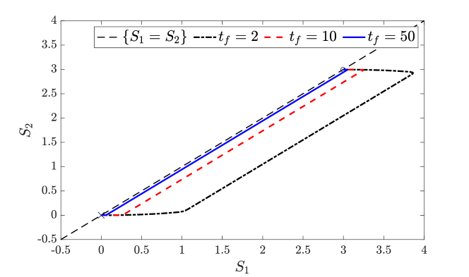
Figure 2. Depiction of the optimal intensive variable $S$ over time (top) and in phase space (bottom) for the heat exchanger

The control constraint set is given by $\mathbb{U}=[-10,10]$ and we aim to perform a state transition between two thermodynamic equilibria: $T_{1}^{0}=T_{2}^{0}=1$ and $T_{1}^{t_{f}}=T_{2}^{t_{f}}=20$. In view of (3.1), the choice of $\alpha_{1}$ in the cost functional does not matter, as the initial and terminal state are fixed. Thus, we choose $\alpha_{1}=0$ and $T_{0}\alpha_{2}=1$.

In view of the optimal control problem (phOCP), this corresponds to the initial value in entropy variables $x^{0}=\begin{pmatrix}0&0\end{pmatrix}^{\top}$ and the terminal set $\Phi=\{\begin{pmatrix}\ln{20}&\ln{20}\end{pmatrix}^{\top}\}$, by means of the relation $T_{i}=e^{S_{i}}$, $i=1,2$. It is clear that this state transition is only possible through providing heat—or, equivalently, entropy—to the first compartment, cf. Figure 1.

In Figure 2, we show the optimal state, control and the Poisson bracket corresponding to entropy creation. It is clear, that we can not perform the state transition in the set of thermodynamic equilibria, as by the form of the input vector in (2.7), no control action that is non-zero leaves $\mathcal{T}$ invariant. However, for increasing time horizons, the state trajectories evolve closer to the manifold, as the necessary rate of entropy supply to perform the state transition in the given horizon can be chosen smaller and smaller. Furthermore, we observe a turnpike behavior of the control towards zero. As mentioned above, this is the only control that leaves the set of thermodynamic equilibria invariant. It can be seen in the upper plot of Figure 2 that the time derivative of the individual entropies in the compartments is constant for the majority of the time. This behavior is called a velocity turnpike and is also central in mechanical sytems with symmetries cf. [9, 26]. Here, this velocity turnpike behavior can can be explained as the Poisson bracket is mostly constant and small—the state has a turnpike towards the manifold—and the control is mostly constant and small—the zero control is the only control that leaves this manifold invariant—and thus the dynamics imply that $\dot{x}_{1}=\dot{S}_{1}\approx\text{const.}$ and $\dot{x}_{2}=\dot{S}_{2}\approx\text{const.}$.

The corresponding extensive variable given by the temperature $H_{x}(S_{1},S_{2})=(T_{1},T_{2})$ in Figure 3. Due to the algebraic relation $T=\exp(S)$, the upper plot of Figure 3 shows exponential evolution of the temperature. Further, as can be observed in the lower plot, he temperature is moving further and further away from the subspace. The reason is that, by means of the turnpike property, we have an optimal rate of travel in the state variable, that is, e.g. for the first compartment, $\text{const.}=\dot{S}_{1}=\tfrac{T_{1}-T_{2}}{T_{1}}$. For increasing temperatures $T_{1}$, the latter fraction can only be constant if also $T_{1}-T_{2}$ increases.

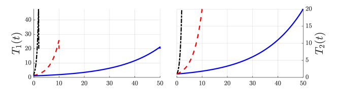
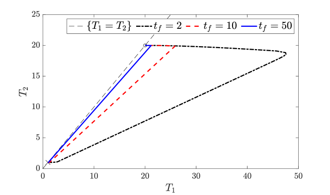
Figure 3. Depiction of the optimal extensive variable $T=H_{x}$ over time (top) and in phase space (bottom) for the heat exchanger

5.2. Stabilization of a heat exchanger

We modify the previous numerical example and do not impose any terminal constraint, i.e., $\Phi=\mathbb{R}^{n}$ and add a output stabilization term to the cost functional in the spirit of Section 4. We aim to track a desired reference temperature of $T_{\mathrm{ref}}=25$ degrees. For the cost functional in (phOCP), we choose $\alpha_{1}=0$ and $T_{0}\alpha_{2}=1$, i.e., we minimize the entropy production. To obtain a linear output of the system state, we translate the aim temperature into an entropy, that is, we aim to minimize, in addition to the entropy creation, the term

$$|S_{2}(t)-S_{\mathrm{ref}}|^{2}=|Cx(t)-S_{\mathrm{ref}}|^{2}$$

with $S_{\mathrm{ref}}=\log(25)$ and $C=\big{[}0\quad 1\big{]}$. Correspondingly, we have $C^{-1}\{S_{\rm ref}\}=\{(S_{1},S_{2})\in\mathbb{R}^{2}:S_{2}=S_{\mathrm{ref}}\}$ which is a one-dimensional affine subspace of $\mathbb{R}^{2}$. In addition, the manifold of thermodynamic equilibria is $\mathcal{T}=\{(S_{1},S_{2})\in\mathbb{R}^{2}:S_{1}=S_{2}\}$. Thus, Theorem 4.2 yields a turnpike w.r.t.

$$C^{-1}\{y_{\rm ref}\}\cap\mathcal{T}=\{(S_{1},S_{2})\in\mathbb{R}^{2}:S_{1}=S_{2}=S_{\mathrm{ref}}\}.$$

This can be observed in Figure 4. There, both entropies appraoch the target entropy $S_{\mathrm{ref}}=\log(25)\approx 3.22$. In order to approach this value, the entropy (or equivalently, the temperature) in the first compartment has to be increased. This yields an increase of the entropy (or temperature) in the second compartment due to the heat flux across the wall, inevitably coupled to entropy generation, cf. bottom left of Figure 4. Having reached the desired target entropy in the second compartment, the control is switched off such that the system is at equilibrium with $u=0$ and no entropy is generated. Thus, both integrands in the cost functional (approximately) vanish for this state: the output term in the cost vanishes as $S_{2}\approx S_{\mathrm{ref}}$ and the entropy production vanishes as $S_{1}=S_{2}$ and thus $\{S,H\}_{J}=T_{1}-T_{2}\approx 0$.

Figure 4. Depiction of the optimal intensive variable, entropy bracket and control over time for output stabilization.

5.3. Set-point transition for a gas-piston system

Last, we consider the gas-piston system of Example 2.7. As an initial configuration of intensive and extensive variables in the thermodynamic domain, we choose

$$S(0)=Ns_{0},\quad V(0)=\frac{NRT_{0}}{P_{0}}$$

such that $\beta(S(0),P(0))=0$ as defined in (2.10) and $T(0)=T_{0}$, $P(0)=P_{0}$. Moreover, we assume that the mechanical subsystem is at equilibrium, that is $v(0)=0$ and $p(0)=0$. The mass is also chosen such that the momentum ODE (last line of (2.12)) is in equilibrium for zero velocity, i.e.,

$$m=\frac{AP_{0}}{g}=5.1644\;\text{kg}.$$

This yields a controlled equilibrium of the system (2.12) endowed with the input map (2.8) when choosing the external temperature $u=T_{0}$. We summarize the chosen parameters in Table 1.

We now aim to steer the piston to the target volume $V(t_{f})=1.3V(0)$ with target zero momentum $p(t_{f})=0$. Analogously to Subsection 5.1 and in view of (3.1), the choice of $\alpha_{1}$ does not matter due to fixed initial and terminal state, such that we set $\alpha_{1}=0$ and $T_{0}\alpha_{2}=1$. The optimal intensive variables, the corresponding extensive quantities, the entropy production by means of the Poisson bracket and the optimal control are depicted in Figure 5.

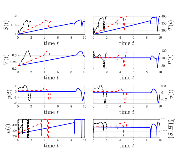
Figure 5. Depiction of the optimal variables for the gas-piston system.

In order to change the volume of the piston, we need to induce a temperature increase by means of the heating jacket. As a result, the volume increases, whereas the pressure stays constant. In view of Theorem 3.11, we observe a turnpike in the velocity component, as $\{S,E\}_{J_{1}}=v$, that is, the manifold of thermodynamic equilibria consists of the states with zero velocity. The longer the time horizon, the smaller the velocity for the majority of the time.

Number of moles $N$	[$-$]	0.01
Reference pressure $P_{0}$	[Pa]	101.325
Reference Temperature $T_{0}$	[K]	273
Reference molar entropy $s_{0}$	[kJ K-1 mol-1]	0.1100
Mass $m$	[kg]	5.1644
Friction coefficient $\nu$	[$-$]	10
Area $A$	[m2]	0.5
heat conduction coeff. $\lambda_{e}$	[$-$]	1

Table 1. Parameters and reference values

5.4. Network of heat exchangers

Last, we present an example with five compartments exchanging heat, which are coupled as depicted in Figure 6.

Figure 6. Network of five compartments exchanging heat.

The corresponding state variables are the entropies in the compartments $S_{i}$, $i=1,\ldots,5$ with Hamiltonian energies $H_{i}(S_{i})=e^{S_{i}}$. $i=1,\ldots,5$. Along the lines of the Example 2.6 and Subsections 5.1 and 5.2 we get by Fourier’s law and continuity of the heat flux for the first, fourth and fifth compartment

$$\lambda_{1}(T_{1}-T_{2}) =-\frac{\mathrm{d}}{\mathrm{d}t}H_{1}(S_{1}(t))=-T_{1}\frac{\mathrm{d}}{\mathrm{d}t}{S}_{1}(t),$$

$$\lambda_{2}(T_{3}-T_{4}) =\phantom{-}\frac{\mathrm{d}}{\mathrm{d}t}H_{4}(S_{4}(t))=\phantom{-}T_{4}\frac{\mathrm{d}}{\mathrm{d}t}{S}_{4}(t),$$

$$\lambda_{3}(T_{3}-T_{5}) =\phantom{-}\frac{\mathrm{d}}{\mathrm{d}t}H_{5}(S_{5}(t))=\phantom{-}T_{5}\frac{\mathrm{d}}{\mathrm{d}t}{S}_{5}(t).$$

For the second compartment, we compute

$$T_{2}\frac{\mathrm{d}}{\mathrm{d}t}{S}_{2}(t)=\frac{\mathrm{d}}{\mathrm{d}t}H_{2}(S_{2}(t))=\lambda_{1}(T_{1}-T_{2})-\lambda_{2}(T_{2}-T_{3}),$$

and for the third compartment,

$$T_{3}\frac{\mathrm{d}}{\mathrm{d}t}{S}_{3}(t)=\frac{\mathrm{d}}{\mathrm{d}t}H_{3}(S_{3}(t))=\lambda_{2}(T_{2}-T_{3})-\lambda_{2}(T_{3}-T_{4})-\lambda_{4}(T_{3}-T_{5}).$$

Thus, corresponding to the four coupling interfaces between the five compartments we define the skew-symmetric structure matrices

$$J_{1} =\begin{bmatrix}0&-1&0&0&0\\ 1&\phantom{-}0&0&0&0\\ 0&\phantom{-}0&0&0&0\\ 0&\phantom{-}0&0&0&0\\ 0&\phantom{-}0&0&0&0\end{bmatrix},\quad J_{2}=\begin{bmatrix}0&0&\phantom{-}0&0&0\\ 0&0&-1&0&0\\ 0&1&\phantom{-}0&0&0\\ 0&0&\phantom{-}0&0&0\\ 0&0&\phantom{-}0&0&0\end{bmatrix},$$

$$J_{3} =\begin{bmatrix}0&0&0&\phantom{-}0&0\\ 0&0&0&\phantom{-}0&0\\ 0&0&0&-1&0\\ 0&0&1&\phantom{-}0&0\\ 0&0&0&\phantom{-}0&0\end{bmatrix},\quad J_{4}=\begin{bmatrix}0&0&0&0&\phantom{-}0\\ 0&0&0&0&\phantom{-}0\\ 0&0&0&0&-1\\ 0&0&0&0&\phantom{-}0\\ 0&0&1&0&\phantom{-}0\end{bmatrix}$$

and the positive functions

$$\gamma_{1}(x,H_{x})=\frac{\lambda_{1}}{T_{1}T_{2}},\qquad\gamma_{2}(x,H_{x})=\frac{\lambda_{2}}{T_{2}T_{3}},$$

$$\gamma_{3}(x,H_{x})=\frac{\lambda_{3}}{T_{3}T_{4}},\qquad\gamma_{4}(x,H_{x})=\frac{\lambda_{3}}{T_{3}T_{5}}.$$

The corresponding Poisson brackets giving rise to the irreversible phenomena read

$$\{S,H\}_{J_{1}}=T_{1}-T_{2},\quad\{S,H\}_{J_{2}}=T_{2}-T_{3},$$

$$\{S,H\}_{J_{3}}=T_{3}-T_{4},\quad\{S,H\}_{J_{4}}=T_{3}-T_{5}.$$

such that

$$\frac{\mathrm{d}}{\mathrm{d}t}S_{1}(t) =-\gamma_{1}(x,H_{x})\{S,H\}_{J_{1}}T_{2},\quad\quad\frac{\mathrm{d}}{\mathrm{d}t}S_{4}(t)=\phantom{-}\gamma_{3}(x,H_{x})\{S,H\}_{J_{3}}T_{3},$$

$$\frac{\mathrm{d}}{\mathrm{d}t}S_{5}(t) =\phantom{-}\gamma_{4}(x,H_{x})\{S,H\}_{J_{4}}T_{3}$$

and

$$\frac{\mathrm{d}}{\mathrm{d}t}S_{2}(t) =\gamma_{1}(x,H_{x})\{S,H\}_{J_{2}}T_{1}-\gamma_{2}(x,H_{x})\{S,H\}_{J_{2}}T_{3}$$

$$\frac{\mathrm{d}}{\mathrm{d}t}S_{3}(t) =\gamma_{2}(x,H_{x})\{S,H\}_{J_{2}}T_{2}-\gamma_{3}(x,H_{x})\{S,H\}_{J_{3}}T_{4}-\gamma_{4}(x,H_{x})\{S,H\}_{J_{4}}T_{5}.$$

Eventually, we obtain with $x=(S_{1},S_{2},S_{3},S_{4},S_{5})$ the dynamics

$$\frac{\mathrm{d}}{\mathrm{d}t}x(t)=\bigg{(}\sum_{i=1}^{4}\gamma_{i}(x,H_{x})\{S,H\}_{J_{i}}J_{i}\bigg{)}H_{x}(x(t)).$$

We endow our system with an a entropy flow control at the first, the fourth and the fifth compartment and aim to track the temperature in these compartments. More precisely, we add the input term

$$g(x,H_{x})u=\begin{bmatrix}1&0&0\\ 0&0&0\\ 0&0&0\\ 0&1&0\\ 0&0&1\end{bmatrix}\begin{bmatrix}u_{1}\\ u_{2}\\ u_{3}\end{bmatrix}$$

and define the output stabilization term

$$\|Cx-y_{\mathrm{ref}}\|^{2}=\left\|\begin{bmatrix}1&0&0&0&0\\ 0&0&0&1&0\\ 0&0&0&0&1\end{bmatrix}x-\begin{bmatrix}S_{1,\mathrm{ref}}\\ S_{4,\mathrm{ref}}\\ S_{5,\mathrm{ref}}\end{bmatrix}\right\|^{2}.$$

for the cost functional. If $S_{1,\mathrm{ref}}\neq S_{4,\mathrm{ref}}$ or $S_{1,\mathrm{ref}}\neq S_{5,\mathrm{ref}}$, then Theorem 4.2 does not apply as

$$C^{-1}\left\{\begin{pmatrix}S_{1,\mathrm{ref}},S_{4,\mathrm{ref}},S_{5,\mathrm{ref}}\end{pmatrix}^{\top}\right\}=\left\{x\in\mathbb{R}^{5}:x_{1}=S_{1,\mathrm{ref}},\,x_{4}=S_{4,\mathrm{ref}},\,x_{5}=S_{5,\mathrm{ref}}\right\}$$

and

$$\mathcal{T}=\left\{x\in\mathbb{R}^{5}:x_{1}=x_{2}=\ldots=x_{5}\right\}$$

such that

$$\begin{split}&C^{-1}\left\{\begin{pmatrix}S_{1,\mathrm{ref}},S_{4,\mathrm{ref}},S_{5,\mathrm{ref}}\end{pmatrix}^{\top}\right\}\cap\mathcal{T}_{\mathrm{opt}}\subset C^{-1}\left\{\begin{pmatrix}S_{1,\mathrm{ref}},S_{4,\mathrm{ref}},S_{5,\mathrm{ref}}\end{pmatrix}^{\top}\right\}\cap\mathcal{T}=\varnothing.\end{split}$$ (5.1)

The results are shown in Figure 7. We see that $S_{1}$, $S_{4}$ and $S_{5}$ do not approach the given reference reference value, as this value would not allow for zero entropy creation. We rather observe a trade-off between the terms in the cost functional: The temperature (or equivalently the entropy) in the fifth and the first compartment is higher than the given reference, whereas in the fourth compartment the temperature is lower as desired. As can be seen in the bottom right plot of Figure 7, also the entropy creation is not small for the majority of the time as we have a trade-off between output stabilization and entropy creation. The reason for this trade-off is that due to (5.1) there is no state for which both terms in the cost functional vanish, which in particular prohibits an application of Theorem 4.2. However, we still can observe a turnpike behavior, which should be investigated in future work.

Figure 7. Entropies in the individual compartments for the network of heat exchangers and generated entropy.

6. Conclusion

We have considered an optimal control problem, intrinsically defined as minimizing the energy supply to the system, the irreversible entropy creation, or a linear combination of both, the minimal exergy destruction. To this end, we have formulated the physical model of the system as a reversible-irreversible port-Hamiltonian system, which is defined w.r.t. a quasi-Poisson bracket and two functions: the total energy acting as a generating function and the total entropy function. We have characterized optimal state-control pairs of the steady state problem in terms of the manifold of thermodynamic equilibria. For dynamic state-transition and output stabilization problems we have derived conditions, under which the optimal solutions of the dynamic problem reside close to the manifold of thermodynamic equilibria for the majority of the time. Last, we have illustrated our results by means of various examples, including purely irreversible systems such as a network of heat exchangers or a reversible-irreversible gas-piston problem consisting of coupled mechanical and thermodynamic systems.

Appendix A Distances

The proof of the following proposition can be found in Appendix A. For a closed convex set $M\subset\mathbb{R}^{n}$ we denote by $P_{M}$ the orthogonal projection onto $M$.

Lemma A.1.

Let $V_{1},\ldots,V_{N}\subset\mathbb{R}^{n}$ be linear subspaces. Then

$$\operatorname{dist}\left(x,\bigcap_{k=1}^{N}V_{k}\right)\,\asymp\,\sum_{k=1}^{N}\operatorname{dist}(x,V_{k})\quad\text{for $x\in\mathbb{R}^{n}$}.$$ (A.1)

Proof.

Since $\operatorname{dist}(x,V_{j})\leq\operatorname{dist}(x,\bigcap_{k=1}^{N}V_{k})$ for $j=1,\ldots,N$, it is evident that the left-hand side of (A.1) is not smaller than $\frac{1}{N}\sum_{k=1}^{N}\operatorname{dist}(x,V_{k})$. Moreover, it obviously suffices to prove the opposite inequality for $N=2$. For this, we set $V=V_{1}$ and $W=V_{2}$. Note that for any subspace $U$ we have $\operatorname{dist}(x,U)=\|P_{U^{\perp}}x\|$.

Suppose that the claim is false. Then there exists a sequence of vectors $(x_{\ell})$ such that for all $\ell\in\mathbb{N}$

$$\|P_{(V\cap W)^{\perp}}x_{\ell}\|\,>\,\ell\big{(}\|P_{V^{\perp}}x_{\ell}\|+\|P_{W^{\perp}}x_{\ell}\|\big{)}.$$

This in particular implies that $y_{\ell}:=P_{(V\cap W)^{\perp}}x_{\ell}\neq 0$. Note that $P_{V^{\perp}}y_{\ell}=P_{V^{\perp}}x_{\ell}$ as $V^{\perp}\subset(V\cap W)^{\perp}$. Setting $z_{\ell}:=y_{\ell}/\|y_{\ell}\|$, it follows that $\|P_{V^{\perp}}z_{\ell}\|+\|P_{W^{\perp}}z_{\ell}\|<\tfrac{1}{\ell}$ for $\ell\in\mathbb{N}$. As $\|z_{\ell}\|=1$ for all $\ell\in\mathbb{N}$, we may assume that $z_{\ell}\to z$ as $\ell\to\infty$ for some vector $z$ with $\|z\|=1$. The latter inequality then shows that $P_{V^{\perp}}z=P_{W^{\perp}}z=0$ and thus $z\in V\cap W$. But $z_{\ell}\in(V\cap W)^{\perp}$ for $\ell\in\mathbb{N}$, which implies $z=0$, contradicting $\|z\|=1$. ∎

Lemma A.2.

Let $V\subset\mathbb{R}^{n}$ be a linear subspace such that $V\cap\mathbb{Y}\neq\varnothing$. Then we have

$$\operatorname{dist}(x,H_{x}^{-1}(V\cap\mathbb{Y}))\,\lesssim\,\operatorname{dist}(H_{x}(x),V),\quad x\in K,$$

for any compact set $K\subset\mathbb{X}$.

Proof.

Suppose that the claim is false. Then there exist a compact set $K\subset\mathbb{X}$ and a sequence $(x_{n})\subset K$ such that

$$\operatorname{dist}(x_{n},H_{x}^{-1}(V\cap\mathbb{Y}))>n\cdot\operatorname{dist}(H_{x}(x_{n}),V),\quad n\in\mathbb{N}.$$

Since $K$ is compact, we may assume WLOG that $x_{n}\to x$ as $n\to\infty$ with some $x\in K$. Set $y_{n}:=H_{x}(x_{n})$ and $y:=H_{x}(x)$. Choose $\varepsilon>0$ such that $\overline{B_{\varepsilon}(y)}\subset\mathbb{Y}$. We have

$$\|P_{V^{\perp}}y_{n}\|=\operatorname{dist}(y_{n},V)<\tfrac{1}{n}\cdot\operatorname{dist}(x_{n},H_{x}^{-1}(V\cap\mathbb{Y}))\to 0$$

and thus also

$$\|y-P_{V}y_{n}\|\leq\|y-y_{n}\|+\|P_{V^{\perp}}y_{n}\|\,\to\,0$$

as $n\to\infty$. Therefore, there exists $n_{0}\in\mathbb{N}$ such that $y_{n},P_{V}y_{n}\in B_{\varepsilon}(y)$ for $n\geq n_{0}$. In particular, for $n\geq n_{0}$ we have $P_{V}y_{n}\in V\cap\mathbb{Y}$ and hence

$$n\|P_{V^{\perp}}y_{n}\| <\operatorname{dist}(H_{x}^{-1}(y_{n}),H_{x}^{-1}(V\cap\mathbb{Y}))\leq\|H_{x}^{-1}(y_{n})-H_{x}^{-1}(P_{V}y_{n})\|$$

$$\leq\Big{[}\sup_{\xi\in[y_{n},P_{V}y_{n}]}\|D_{\xi}H_{x}^{-1}\|\Big{]}\cdot\|y_{n}-P_{V}y_{n}\|\leq\Big{[}\sup_{\xi\in\overline{B_{\varepsilon}(y)}}\|D_{\xi}H_{x}^{-1}\|\Big{]}\cdot\|P_{V^{\perp}}y_{n}\|,$$

which is a contradiction for large $n$. ∎

Proof of Proposition 3.8.

First of all, note that $\{S,H\}_{J_{k}}(x)=-H_{x}(x)^{\top}J_{k}e$ for $k=1,\ldots,N$. In particular, $\mathcal{T}=H_{x}^{-1}(V\cap\mathbb{Y})$. Also, $|w^{\top}v|=\|v\|\operatorname{dist}(w,v^{\perp})$ for $v,w\in\mathbb{R}^{n}$. Hence, by Lemmas A.1 and A.2,

$$\operatorname{dist}(x,\mathcal{T}) =\operatorname{dist}(x,H_{x}^{-1}(V\cap\mathbb{Y}))\,\lesssim\,\operatorname{dist}(H_{x}(x),V)$$

$$\lesssim\sum_{k=1}^{N}\operatorname{dist}(H_{x}(x),(J_{k}e)^{\perp})\lesssim\sum_{k=1}^{N}\|J_{k}e\|\cdot\operatorname{dist}(H_{x}(x),(J_{k}e)^{\perp})$$

$$=\sum_{k=1}^{N}|H_{x}(x)^{\top}J_{k}e|=\sum_{k=1}^{N}|\{S,H\}_{J_{k}}(x)|.$$

Note that this also holds if $J_{k}e=0$ for some $k$. Finally, squaring left- and right-hand side of the latter inequality and applying Cauchy-Schwarz, the claim follows from the fact that there is some $c>0$ such that $\gamma_{k}(x,H_{x}(x))\geq c$ for $x\in K$ and all $k=1,\ldots,N$. ∎

References

- [1] A. A. Alonso and B. E. Ydstie. Process systems, passivity and the second law of thermodynamics. Computers & chemical engineering, 36:10, 1996.
- [2] A. A. Alonso, B. E. Ydstie, and J. R. Banga. From irreversible thermodynamics to a robust control theory for distributed process systems. Journal of Process Control, 12:507–517, 2002.
- [3] F. Couenne, C. Jallut, B. Maschke, P. Breedveld, and M. Tayakout. Bond graph modelling for chemical reactors. Mathematical and Computer Modelling of Dynamical Systems, 12:2, June 2006.
- [4] T. Damm, L. Grüne, M. Stieler, and K. Worthmann. An exponential turnpike theorem for dissipative discrete time optimal control problems. SIAM Journal on Control and Optimization, 52(3):1935–1957, 2014.
- [5] G. De Koeijer and S. Kjelstrup. Minimizing entropy production rate in binary tray distillation. International Journal of Thermodynamics, 3(3):105–110, 2000.
- [6] V. Duindam, A. Macchelli, S. Stramigioli, and H. Bruyninckx. Modeling and Control of Complex Physical Systems - The Port-Hamiltonian Approach. Springer Berlin, Heidelberg, 2009.
- [7] D. Eberard, B. M. Maschke, and A. van der Schaft. An extension of Hamiltonian systems to the Thermodynamic space: towards a geometry of non-equilibrium Thermodynamics. Reports on Mathematical Physics, 60(2):175–198, 2007.
- [8] T. Faulwasser, K. Flaßkamp, S. Ober-Blöbaum, M. Schaller, and K. Worthmann. Manifold turnpikes, trims, and symmetries. Mathematics of Control, Signals, and Systems, pages 1–30, 2022.
- [9] T. Faulwasser, K. Flaßkamp, S. Ober-Blöbaum, and K. Worthmann. A dissipativity characterization of velocity turnpikes in optimal control problems for mechanical systems. IFAC-PapersOnLine, 54(9):624–629, 2021.
- [10] T. Faulwasser and L. Grüne. Turnpike properties in optimal control: An overview of discrete-time and continuous-time results. In E. Zuazua and E. Trelat, editors, Handbook of Numerical Analysis, volume 23, chapter 11, pages 367–400. Elsevier, 2022.
- [11] T. Faulwasser, J. Kirchhoff, V. Mehrmann, F. Philipp, M. Schaller, and K. Worthmann. Hidden regularity in singular optimal control of port-Hamiltonian systems. Submitted, preprint arXiv:2305.03790, 2023.
- [12] T. Faulwasser, M. Korda, C. N. Jones, and D. Bonvin. On turnpike and dissipativity properties of continuous-time optimal control problems. Automatica, 81:297–304, 2017.
- [13] T. Faulwasser, B. Maschke, F. Philipp, M. Schaller, and K. Worthmann. Optimal control of port-Hamiltonian descriptor systems with minimal energy supply. SIAM Journal on Control and Optimization, 60(4):2132–2158, 2022.
- [14] A. Favache, D. Dochain, and B. M. Maschke. An entropy-based formulation of irreversible processes based on contact structures,. Chemical Engineering Science, 65:5204–5216, 2010.
- [15] A. Favache, B. M. D. Santos, V. Maschke, and D. Dochain. Some properties of conservative control systems. IEEE trans. on Automatic Control, 54(10):2341–2351, 2009.
- [16] J. P. García-Sandoval, N. Hudon, and D. Dochain. Generalized Hamiltonian representation of thermo-mechanical systems based on an entropic formulation. Journal of Process Control, 51:18–26, 2017.
- [17] J. P. García-Sandoval, N. Hudon, D. Dochain, and V. González-Alvarez. Stability analysis and passivity properties of a class of thermodynamic processes: An internal entropy production approach. Chemical Engineering Science, 139:261–272, 2016.
- [18] H. Hoang, F. Couenne, C. Jallut, and Y. L. Gorrec. The port Hamiltonian approach to modeling and control of Continuous Stirred Tank Reactors. Journal of Process Control, 21(10):1449–1458, 2011.
- [19] H. Hoang, F. Couenne, C. Jallut, and Y. L. Gorrec. Lyapunov-based control of non isothermal continuous stirred tank reactors using irreversible thermodynamics. Journal of Process Control, 22(2):412–422, 2012.
- [20] E. Johannessen and S. Kjelstrup. Minimum entropy production rate in plug flow reactors: An optimal control problem solved for SO2 oxidation. Energy, 29(12):2403–2423, 2004.
- [21] A. Karsai. Manifold turnpikes of nonlinear port-Hamiltonian descriptor systems under minimal energy supply. arXiv:2301.09094, 2023.
- [22] B. Maschke and J. Kirchhoff. Port maps of Irreversible Port Hamiltonian Systems, 2022. to appear Proc. IFAC World Congress, Yokohama, Japan, 9 July - 14 July 2023, preprint: arXiv:2302.09026.
- [23] B. Maschke, F. Philipp, M. Schaller, K. Worthmann, and T. Faulwasser. Optimal control of thermodynamic port-Hamiltonian systems. IFAC-PapersOnLine, 55(30):55–60, 2022.
- [24] H. C. Öttinger. Nonequilibrium thermodynamics for open systems. Physical Review E, 73:036126, March 2006.
- [25] F. Philipp, M. Schaller, T. Faulwasser, B. Maschke, and K. Worthmann. Minimizing the energy supply of infinite-dimensional linear port-Hamiltonian systems. IFAC-PapersOnLine, 54(19):155–160, 2021.
- [26] D. Pighin and N. Sakamoto. The turnpike with lack of observability, 2020. arXiv:2007.14081.
- [27] H. Ramirez. Control of irreversible thermodynamic processes using port-Hamiltonian systems defined on pseudo-Poisson and contact structures. PhD thesis, Université Claude Bernhard Lyon 1, 2012.
- [28] H. Ramirez, Y. L. Gorrec, B. Maschke, and F. Couenne. On the passivity based control of irreversible processes: A Port-Hamiltonian approach. Automatica, 64:105–111, 2016.
- [29] H. Ramirez, B. Maschke, and D. Sbarbaro. Feedback equivalence of input-output contact systems. Systems & Control Letters, 62(6):475–481, 2013.
- [30] H. Ramirez, B. Maschke, and D. Sbarbaro. Irreversible port-Hamiltonian systems: A general formulation of irreversible processes with application to the CSTR. Chemical Engineering Science, 89:223–234, 2013.
- [31] H. Ramirez, B. Maschke, and D. Sbarbaro. Modelling and control of multi-energy systems: An irreversible Port-Hamiltonian approach. European Journal of Control, 19(6):513–520, 2013.
- [32] H. Ramirez, B. Maschke, and D. Sbarbaro. Partial stabilization of input-output contact systems on a Legendre submanifold. IEEE Transactions on Automatic Control, 62(3):1431–1437, March 2017.
- [33] M. Ruszkowski, V. Garcia-Osorio, and B. E. Ydstie. Passivity based control of transport reaction systems. AIChE journal, 51(12):3147–3166, December 2005.
- [34] M. Schaller, F. Philipp, T. Faulwasser, K. Worthmann, and B. Maschke. Control of port-Hamiltonian systems with minimal energy supply. European Journal of Control, 62:33–40, 2021. Special issue on the European Control Conference 2021.
- [35] E. Trélat and E. Zuazua. The turnpike property in finite-dimensional nonlinear optimal control. Journal of Differential Equations, 258(1):81–114, 2015.
- [36] A. van der Schaft. Geometric modeling for control of thermodynamic systems. Entropy, 25(4), 2023.
- [37] A. van der Schaft and D. Jeltsema. Port-Hamiltonian systems theory: An introductory overview. Foundations and Trends in Systems and Control, 1(2-3):173–378, 2014.
- [38] A. van der Schaft and B. Maschke. Geometry of Thermodynamic Processes. Entropy, 20(12):925–947, 2018.
- [39] L. Wang, B. Maschke, and A. Van Der Schaft. Stabilization of control contact systems. IFAC-PapersOnLine, 48(13):144–149, 2015.
- [40] Ø. Wilhelmsen, E. Johannessen, and S. Kjelstrup. Entropy production minimization with optimal control theory. In Experimental Thermodynamics Volume X, pages 271–289. 2015.
- [41] E. Zeidler. Nonlinear Functional Analysis and its Applications IV: Applications to Mathematical Physics. Springer New York, NY, 1988.
- [42] S. Zenfari, M. Laabissi, and M. E. Achhab. Observer design for a class of irreversible port Hamiltonian systems. An International Journal of Optimization and Control: Theories & Applications, 13(1):26–34, 2023.