SplatFlow: Learning Multi-frame Optical Flow via Splatting

Abstract

Occlusion problem remains a key challenge in Optical Flow Estimation (OFE) despite the recent significant progress brought by deep learning in the field. Most existing deep learning OFE methods, especially those based on two frames, cannot properly handle occlusions, in part because there is no significant feature similarity in occluded regions. The multi-frame settings have the potential to mitigate the occlusion issue in OFE. However, the problem of Multi-frame OFE (MOFE) remains underexplored, and the limited works are specially designed for pyramid backbones and obtain the aligned temporal information by time-consuming backward flow calculation or non-differentiable forward warping transformation. To address these shortcomings, we propose an efficient MOFE framework named SplatFlow, which is realized by introducing the differentiable splatting transformation to align the temporal information, designing a One-to-Many embedding method to densely guide the current frame’s estimation, and further remodelling the existing two-frame backbones. The proposed SplatFlow is very efficient yet more accurate as it is able to handle occlusions properly. Extensive experimental evaluations show that our SplatFlow substantially outperforms all published methods on KITTI2015 and Sintel benchmarks. Especially on Sintel benchmark, SplatFlow achieves errors of 1.12 (clean pass) and 2.07 (final pass), with surprisingly significant 19.4% and 16.2% error reductions from the previous best results submitted, respectively. Code is available at https://github.com/wwsource/SplatFlow.

1 Introduction

Optical Flow Estimation (OFE) aims at estimating the pixel-wise 2D motion between consecutive video frames. As a longstanding, fundamental yet challenging problem in low-level vision Horn and Schunck (1981); Gibson (1950), OFE has been extensively studied for several decades due to its numerous applications, including video object segmentation Cheng et al. (2017), video object tracking Aslani and Mahdavi-Nasab (2013), VSLAM Choi et al. (2014), action recognition Sevilla-Lara et al. (2018), 3D reconstruction Li et al. (2019), video inpainting Xu et al. (2019); Gao et al. (2020), video superresolution Sajjadi et al. (2018), depth estimation Ranftl et al. (2016), scene flow estimation Yang and Ramanan (2020), and many others. Before the deep learning era, variational approaches had dominated the field of OFE since the work by Horn and Schunck Horn and Schunck (1981).

Recently, akin to many vision problems, the boom of deep learning has injected new vitality into the field of OFE, causing the research focus to transfer from traditional methods Brox et al. (2009); Horn and Schunck (1981); Xu et al. (2011) to deep learning Dosovitskiy et al. (2015); Ilg et al. (2017); Sun et al. (2018); Teed and Deng (2020). Indeed, deep learning based methods like PWC-Net Sun et al. (2018) and RAFT Teed and Deng (2020) have achieved higher accuracy than the best classical methods Revaud et al. (2015); Weinzaepfel et al. (2013); Bailer et al. (2015) while being significantly faster at inference time. Despite the tremendous progress brought by deep learning, most OFE methods have not been, however, capable of performing at a level sufficient for realistic applications due to various challenges, including the followings.

• High computational cost. Most advanced deep learning based methods Teed and Deng (2020); Jiang et al. (2021a); Zhang et al. (2021) perform OFE based on a correlation volume that stores the pairwise pixel similarities between two frames. Clearly, the computation grows quadratically with the number of pixels in a frame Jiang et al. (2021b). In addition, most such methods are constrained to be deployed in resource-limited edge devices.

• High cost of collecting large-scale labelled data. Collecting large-scale, densely labelled, realistic data for OFE is prohibitively costly. Most current methods use synthetic data Mayer et al. (2016); Butler et al. (2012) for training, leading to decreased accuracy on realistic data due to the domain gap Liu et al. (2019). Therefore, many unsupervised Wang et al. (2018); Jonschkowski et al. (2020) or self-supervised Liu et al. (2019) methods have been explored to address this challenge.

• Occlusion. Occlusion is an inevitable and important problem in OFE. The existence of occlusion has a major impact on accuracy, as matching costs are not accessible in occluded regions. Proper occlusion handling plays a critical role in accurate OFE.

To further improve OFE performance, we realize that occlusion is among the major factors that limit the popular deep learning based methods. In addition, the accurate OFE in occluded regions is beneficial for high-level visual tasks, which could provide the basic spatial relationships of objects in the scene and realize the complete motion tracking of objects. In this paper, we intend to carefully address the occlusion issue.

Existing popular deep learning based OFE methods are based on two consecutive frames, which have inherent limitations in handling occlusions. Under the two-frame settings, the networks directly match or indirectly regress each pixel’s optical flow according to the significant feature similarity between pixel pairs. Unfortunately, this idea is not feasible in occlusions. The occluded regions will be occluded by other regions in the next frame, or move out of the image boundary. In this case, the feature similarity values will be generally low for occluded regions due to no good correspondences, therefore leading to failed estimations. Although Jiang et al. Jiang et al. (2021a) proposed that the flow in non-occluded regions in the current frame can be aggregated by feature similarity, which can be used as a reference for estimating the optical flow in occluded regions, this method can only solve a very small part of occlusions. In most cases, occluded regions cannot find a reference with high feature similarity in the current frame.

As aforementioned, handling occlusions is very challenging under the two-frame settings. One straightforward way is to consider multiple frames by exploring temporal smoothness. Obviously, the multi-frame settings provide richer information, enable the exploration of different kinds of assumptions and have the potential to mitigate the occlusion issue. However, introducing more frames raises more difficulties, such as potential harmfulness under dramatic changes of flow field Volz et al. (2011), accumulation and diffusion of errors from the previous frame’s estimation, and higher computational costs Irani (1999); Wulff et al. (2017). Currently, the problem of Multi-frame Optical Flow Estimation (MOFE) remains underexplored, with only very few works Ren et al. (2019); Neoral et al. (2018); Liu et al. (2019) which have the following limitations.

• Few specialized multi-frame methods for the advanced single-resolution iterative two-frame backbones. The existing deep learning multi-frame methods are mainly divided into two types: Methods Neoral et al. (2018); Liu et al. (2019) specially designed for pyramidal backbones and methods Ren et al. (2019); Maurer and Bruhn (2018) agnostic to backbones. The former cannot adapt to the advanced single-resolution iterative backbones, e.g., RAFT Teed and Deng (2020) and GMA Jiang et al. (2021a). The latter often can not make full use of the backbone network’s characteristics, so they can only achieve sub-optimal estimation performance or sometimes can not outperform two-frame methods. As far as we know, the WarmStart initialization proposed in RAFT Teed and Deng (2020) is the only method specially designed for the single-resolution iterative backbones. Unfortunately, this initialization method still cannot effectively handle occlusions.

• Limitations of the commonly used temporal information alignment methods. The information of the history frame has a coordinate system different from the current frame. Most existing methods obtain the aligned temporal information, which will be embedded into the two-frame backbones, by performing the inference process of backward flow from the current frame to the previous frame or performing a non-differentiable forward warping transformation. However, as a most direct way, computing the backward flow will increase the computational cost at least twice, which will seriously affect the real-time performance of the algorithm. Using a non-differentiable forward warping transformation makes the network unable to propagate gradient through this step, thus hindering the effective learning of multi-frame knowledge during training.

In this paper, we propose a theoretically very simple yet efficient MOFE framework, dubbed SplatFlow, that specifically targets the occlusion problem. The novelty of our method stands on careful consideration of the unique “single-resolution” characteristic of the current advanced two-frame backbones, the drawbacks of high cost in backward flow calculation, and the limitations of non-differentiability in commonly used forward warping transformation, and is realized by introducing the differentiable splatting transformation to align the temporal information, designing a One-to-Many embedding method to densely guide the current frame’s estimation, and further remodelling the existing two-frame backbones.

In specific, our proposed SplatFlow framework builds a feedforward propagation bridge for the historical frame’s temporal information to be embedded into the current frame’s OFE process. The framework includes three parts: encoding, alignment, and embedding of the temporal information. Firstly, we use the joint motion feature (JMF), which is the joint convolutional coding feature of flow and correlation feature, as the temporal information type of our framework. Secondly, we propose a splatting-based temporal information alignment method to replace backward flow calculation or non-differentiable forward warping transformation. Here we introduce the splatting transformation widely used in the field of video frame interpolation into the application of MOFE. The previous frame’s temporal information, i.e., JMF, is injected with bi-linear weights into the adjacent four pixels of the target sub-pixel position calculated by the previous frame’s optical flow, thus achieving a differentiable and forward temporal information alignment at the sub-pixel level. Finally, we specially design a One-to-Many temporal information embedding method for the advanced two-frame backbones. Specifically, the network selects the optimal aligned temporal information (One) based on specific rules and further densely embeds it into every iteration (Many) of the current frame’s estimation process.

The whole SplatFlow framework is highly adapted to the advanced single-resolution iterative two-frame backbone networks, e.g., RAFT Teed and Deng (2020) and GMA Jiang et al. (2021a). Compared with the original two-frame backbone, our method has significantly higher estimation accuracy, especially in occluded regions, while maintaining a comparable inference speed. At the time of submission, our method achieved the state-of-the-art results on the authoritative and challenging Sintel benchmark Butler et al. (2012), with surprisingly significant 19.4% (clean pass) and 16.2% (final pass) error reductions compared to the previous best result submitted. Besides, our method also outperformed all published pure optical flow methods on KITTI2015 benchmark Menze and Geiger (2015).

The contributions of this paper are summarized as follows:

• We propose a novel MOFE framework SplatFlow for the advanced single-resolution iterative two-frame backbones. Compared with the original backbone, SplatFlow has significantly higher estimation accuracy, especially in occluded regions, while maintaining a high inference speed.

• In our framework, we propose a splatting-based temporal information alignment method to replace the commonly used backward flow calculation or non-differentiable forward warping transformation, thus achieving a differentiable and forward temporal information alignment at the sub-pixel level.

• In our framework, we specially design a One-to-Many temporal information embedding method to make full use of the backbone’s unique “single-resolution” characteristic and maximize the guiding role of the temporal information.

• At the time of submission, our SplatFlow achieved the state-of-the-art results on both Sintel Butler et al. (2012) and KITTI2015 Menze and Geiger (2015) benchmarks, especially with surprisingly significant 19.4% (clean pass) and 16.2% (final pass) error reductions compared to the previous best result submitted on Sintel Butler et al. (2012) benchmark.

2 Related Work

2.1 Two-frame Deep Learning Methods

Thanks to the successful experiences of the DNNs in various computer vision tasks, the OFE methods based on deep learning gradually surpass the traditional methods both in accuracy and speed. FlowNet Dosovitskiy et al. (2015) is the first method using DNNs to estimate optical flow. By stacking a series of warping operations, FlowNet2.0 Ilg et al. (2017) performs on par with the state-of-the-art methods. After that, a series of methods, such as PWC-Net Sun et al. (2018) and LiteFlowNet Hui et al. (2018), adopt a pyramid structure and refine the estimated optical flow from coarse to fine. This coarse-to-fine cascade has several limitations, such as the difficulty of recovering from errors at coarse resolutions and the tendency to miss small fast-moving objects, as described and addressed in RAFT Teed and Deng (2020). RAFT Teed and Deng (2020) adopts an iterative method to continuously refine the results of optical flow at the same high resolution and has achieved great performance improvements. Since then, many works Jiang et al. (2021a, b); Xu et al. (2021) have optimized this single-resolution iterative two-frame backbone from the perspective of reducing computational costs or improving the accuracy. Among them, GMA Jiang et al. (2021a) is dedicated to solving occlusions under the two-frame settings. It uses the attention mechanism to capture motion clues from similar areas in the spatial domain corresponding to the current frame. However, this can only solve the special cases of a very small part of occlusions.

2.2 Multi-frame Deep Learning Methods

To deal with occlusions more comprehensively, some studies enable the network to extract and fuse the temporal information under the multi-frame settings.

FusionFlow Ren et al. (2019) uses the temporal information to non-iteratively optimize the two-frame method’s full-resolution optical flow results, and it does not depend on specific backbone network types. This method has good generality and is suitable for all kinds of two-frame backbones. However, it only performs post-processing, i.e., fusion operation, for the two-frame estimation results and does not use the temporal information for preliminary guidance. Therefore, it can only achieve sub-optimal performance compared with the following specialized multi-frame methods. Besides, Proflow Maurer and Bruhn (2018), which is closely related to FusionFlow Ren et al. (2019), was proposed, but the algorithm does not outperform two-frame methods on many datasets.

For a coarse-to-fine network structure, the self-supervise method SelFlow Liu et al. (2019) uses the forward correlation volume of the previous frame and the backward low-resolution optical flow as the temporal information to refine each layer’s OFE result. Similarly, ContinualFlow Neoral et al. (2018) also embeds the temporal information into the process of restoring a higher-resolution optical flow. However, it uses forward and backward warped optical flow as the temporal information rather than the forward correlation volume. According to the characteristics of the pyramid backbone networks, the above methods cleverly embed the temporal information into the refinement of the resolution from coarse to fine, which greatly improves the network’s utilization effect of the temporal information. The aforementioned multi-frame methods are difficult to apply directly to the current advanced two-frame networks such as RAFT Teed and Deng (2020), GMA Jiang et al. (2021a).

As far as we know, the WarmStart initialization proposed in RAFT Teed and Deng (2020) is the only method for the advanced single-resolution iterative two-frame backbone networks. It forward projects the previous frame’s optical flow to the current frame to replace zero as the initial value of the optical flow iterations. However, this early one-time temporal information injection will be forgotten after a large number of GRU iterations, so it still cannot effectively handle occlusions.

2.3 Warping Transformations

Figure 1: The overall architecture of the proposed SplatFlow framework which is designed for the single-resolution iterative backbone, e.g., RAFT Teed and Deng (2020). The brown and black arrows show the estimation processes $P_{t-1\rightarrow t}$ and $P_{t\rightarrow t+1}$, respectively. The framework includes three parts: encoding, alignment, and embedding of the temporal information. The encoder network encodes JMF as the type of the temporal information (green part). We use a splatting-based method to realize a unidirectionally and differentiable alignment of the temporal information (blue part). We use a One-to-Many embedding method to densely guide the frame $t$’s estimation process with the selected optimal aligned temporal information (red part). The detailed data flow for iteratively updating optical flow in RAFT Teed and Deng (2020) is summarized as Single-resolution Iteration Module (SIM) in the purple part.

Given two adjacent image frames $I_{1}$ and $I_{2}$, backward warping transformation refers to mapping $I_{2}$ using the optical flow from $I_{1}$ to $I_{2}$ through an image sampling operation Jason et al. (2016) to reconstruct $I_{1}$. The commonly used sampling mode is the bi-linear sampling. The backward warping transformation is differentiable and is widely used in unsupervised optical flow estimation Meister et al. (2018); Wang et al. (2018), supervised optical flow estimation Sun et al. (2018); Hui et al. (2018), unsupervised depth estimation Godard et al. (2017); Mahjourian et al. (2018), novel view synthesis Cun et al. (2018); Liu et al. (2018), video frame interpolation Bao et al. (2019); Jiang et al. (2018), and video enhancement Tao et al. (2017); Caballero et al. (2017).

When backward warping transformation is applied to multi-frame optical flow methods Neoral et al. (2018); Ren et al. (2019), the backward flow from $I_{2}$ to $I_{1}$ is generally used to map the image, flow, or other features corresponding to $I_{1}$ to align with the $I_{2}$’s coordinate system. After that, the backward warped features could provide the temporal information of the previous frame $I_{1}$, and be input into the network for estimating the optical flow of the current frame $I_{2}$.

Forward warping transformation is mainly used in OFE Wang et al. (2018); Neoral et al. (2018) and video frame interpolation Niklaus and Liu (2018); Bao et al. (2019); Niklaus and Liu (2020). In forward warping transformation, the feature’s mapping direction is consistent with the optical flow’s direction, which is different from backward warping transformation. Specifically, when mapping $I_{1}$ to $I_{2}$, the optical flow from $I_{1}$ to $I_{2}$ is used to provide targets’ positions instead of that from $I_{2}$ to $I_{1}$.

The consistency of directions brings forward warping transformation some great challenges, which include the conflict of mapping multiple sources to the same target and non-differentiability problems. To capture the temporal information from the previous frame’s optical flow, ContinualFlow Neoral et al. (2018) retains the maximum flow value at the same mapped target during mapping. However, since this warping is not differentiable and the network cannot propagate gradients through this step during training, therefore this warping proved useless in the experiments. The same problem occurs with CtxSyn Niklaus and Liu (2018), which uses the equivalent of z-buffering. In unsupervised optical flow estimation, Wang et al.Wang et al. (2018) propose a differentiable method: taking the sum of contributions from all source pixels to the same target as the mapped value, which is also known as splatting and widely used in the field of video frame interpolation Niklaus and Liu (2020); Hu et al. (2022); Siyao et al. (2021).

To the best of our knowledge, we are the first to introduce the differentiable splatting transformation into MOFE.

3 Proposed Method

In this section, the holistic architecture of our method is described in subsection 3.1, and then the key contributions of our method, including the Splatting-based temporal information alignment method and the One-to-Many temporal information embedding method, are depicted in subsections 3.2 and 3.3, respectively. Some details of the model during training and inference are provided in subsection 3.4.

3.1 Overall Architecture of SplatFlow

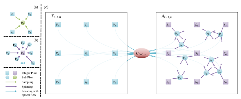
Figure 2: (a) Schematic illustration of sampling. (b) Schematic illustration of splatting. (c) Schematic illustration of the proposed splatting-based temporal information alignment method.

Our multi-frame method is designed for single-resolution iterative two-frame backbone networks such as RAFT Teed and Deng (2020) and GMA Jiang et al. (2021a). Here we take RAFT Teed and Deng (2020) as an example to introduce the overall architecture of our method, and the architecture is illustrated in Fig. 1.

The brown and black arrows in Fig. 1 show the OFE processes $P_{t-1\rightarrow t}$ (from the frame $t-1$ to $t$) and $P_{t\rightarrow t+1}$ (from the frame $t$ to $t+1$) of the original RAFT Teed and Deng (2020), respectively. The two processes have the same network structure and data flow except for different inputs. The $P_{t\rightarrow t+1}$ process takes two adjacent images $I_{t}$ and $I_{t+1}$ as inputs, and extracts the image feature $F^{i}$ and the context feature $F^{c}$ of each image with a feature encoder and context encoder networks that have identical structures but independent parameters. The 4-layer correlation pyramid $Y_{t}$ between $F^{i}_{t}$ and $F^{i}_{t+1}$ is calculated by taking the dot product between all pairs of feature vectors and pooling the last two dimensions. Then, $Y_{t}$ and $F^{c}_{t}$ are used as inputs to update the low-resolution optical flow estimates $O_{t}$ with an initial value of 0 through an iterative method, which is shown as Single-resolution Iteration Module (SIM) in the purple part of Fig. 1, and the full-resolution result $O^{f}_{t}$ is recovered by using convex upsampling Teed and Deng (2020). During the $n^{th}$ iteration of the GRU Predictor network in SIM, the correlation feature $C_{t,n}$ is generated by dynamically looking up $Y_{t}$ with $O_{t,n-1}$ and a separable convolutional GRU Unit is used to input $C_{t,n}$, $O_{t,n-1}$ and $F^{c}_{t}$ to predict a low-resolution optical flow residual $\Delta O_{t,n}$ for updating $O_{t,n-1}$ to $O_{t,n}$.

Our SplatFlow multi-frame optical flow framework builds a feedforward propagation bridge for the $P_{t-1\rightarrow t}$ process’s information to be embedded into the $P_{t\rightarrow t+1}$ process. The SplatFlow framework firstly extracts the specific type of the temporal information feature, i.e., $T_{t-1,n}$, after each iteration of the $P_{t-1\rightarrow t}$ process, and takes a specific alignment method to obtain the temporal information feature aligned with the frame $t$’s coordinate system, i.e., $A_{t-1,n}$. Then the framework uses a specific embedding method to use the aligned temporal information features to guide estimation during the $P_{t\rightarrow t+1}$ process.

The green part in Fig. 1 shows the Temporal Information Encoder network in our framework. We introduce the JMF from the two-frame method RAFT Teed and Deng (2020) as the temporal information type of our framework. Specifically, the network jointly encodes the $C_{t-1,n}$ and $O_{t-1,n-1}$ generated in each iteration of the $P_{t-1\rightarrow t}$ process, and obtains $T_{t-1,n}$.

We use the Splatting-based Aggregator network to implement our proposed Splatting-based temporal information alignment method, as shown in the blue part in Fig. 1. After extracting the $T_{t-1,n}$ of each iteration, we use $O_{t-1,n}$ to map it unidirectionally to the coordinate system of the frame $t$ to obtain $A_{t-1,n}$. Based on the splatting transformation, differentiable and sub-pixel level filling of the temporal information features can be realized.

The red part in Fig. 1 shows the One-to-Many Embedder network in our framework. It uses the Optimal Selector module based on specific rules to select the optimal aligned temporal information feature $A^{*}_{t-1}$ in feature set $S=\{A_{t-1,1},A_{t-1,2},...,A_{t-1,n}\}$. After that, $A^{*}_{t-1}$ is densely embedded into each iteration of the $P_{t\rightarrow t+1}$ process, guiding each update of $O_{t,n}$ by providing an optimal motion priori.

3.2 Splatting-based Alignment Method

The temporal information feature just extracted from the frame $t-1$ can not directly guide the frame $t$’s OFE, because its coordinate system is not aligned with the frame $t$. On the contrary, if the temporal information feature comes from the frame $t$’s backward flow estimation process, this problem will not be encountered, but the computational cost will be multiplied. In order to align the temporal information efficiently, we introduce the differentiable forward warping transformation, namely splatting, from the field of video frame interpolation Niklaus and Liu (2020).

Splatting is the inverse operation of sampling. Fig. 2 (a) and (b) show the relationship between the two. The four rectangles in Fig. 2 (a) represent adjacent integer pixels in an image, and their pixel values are $V_{1}$, $V_{2}$, $V_{3}$ and $V_{4}$, respectively. The circle in the middle of them represents the sub-pixel to be sampled, and its pixel value is $V_{0}$.

When bi-linear sampling is used, $V_{0}$ can be expressed as the weighted sum of adjacent four integer pixel values. The mathematical expression is as follows,

$$V_{0}=\sum_{i=1}^{4}w_{i}V_{i},$$ (1)

$$w_{i}=(1-\Delta x_{i})(1-\Delta y_{i}),,$$ (2)

$$\Delta x_{i}=|x_{i}-x_{0}|,$$ (3)

$$\Delta y_{i}=|y_{i}-y_{0}|,$$ (4)

where $x_{i}$ and $y_{i}$ are the x and y coordinates of the pixel $i$.

From Eq. (2), (3) and (4), it can be deduced that the four weights here have the following relationship,

$$\sum_{i=1}^{4}w_{i}=1.$$ (5)

Therefore, Eq. (1) can be written in the following form,

$$V_{0}=\sum_{i=1}^{4}n_{i}V_{i},$$ (6)

$$n_{i}=\frac{w_{i}}{\sum_{i=1}^{4}w_{i}}=w_{i}.$$ (7)

From Eq. (6) and (7), it can be concluded that sampling a sub-pixel is computing the normalized weighted sum of the values of all adjacent integer pixels. The inverse of this conclusion is splatting; that is, splatting an integer pixel is computing the normalized weighted sum of the values of all adjacent sub-pixels (Note that the first splatting proposed by Wang et al.Wang et al. (2018) uses a non-normalized weighted sum, which leads to brightness inconsistencies Niklaus and Liu (2020)). The mathematical expression is as follows,

$$V_{0}=\sum_{i=1}^{k}n_{i}V_{i},$$ (8)

$$n_{i}=\frac{f(w_{i})}{\sum_{i=1}^{k}f(w_{i})},$$ (9)

$$w_{i}=max(0,1-\Delta x_{i})\cdot max(0,1-\Delta y_{i}).$$ (10)

Here, $k$ is the number of all sub-pixels in an image. We guarantee the contribution of all sub-pixels, whose distance exceeds 1 pixel, is zero by taking $max(\cdot)$ operation in Eq. (10). $f(\cdot)$ is a mapping operation to $w_{i}$. Fig. 2 (b) shows the schematic illustration of splatting, in which the middle rectangle represents the integer pixel to be splatted, and the surrounding circles are all sub-pixels.

The differences of $f(\cdot)$s determine how the splatting algorithm handles conflicts that multiple sources map to the same target. Different $f(\cdot)$s of commonly used splatting types, such as average splatting and softmax splatting Niklaus and Liu (2020), are listed in Eq. (11) and (12), respectively:

$$f^{a}(w_{i})=w_{i},$$ (11)

$$f^{s}(w_{i})=exp(Z_{i})\cdot w_{i},$$ (12)

where $Z$ is an importance metric which can measure the mapping priority of the source. Most intuitively, $Z$ can represent the inverse depth of the sub-pixel; that is, the bigger the depth, the more likely it will be occluded and covered by other sources. However, depth is often difficult to obtain. An alternative Niklaus and Liu (2020) is to use the feature similarity between source and target as $Z$. Compared with average splatting, softmax splatting can not only strengthen the mapping ability of the high-importance source, but also realize the translation invariance of importance. Therefore, it works best in theory to resolve conflicts.

Based on the idea of splatting, we propose a new temporal information alignment method. We use $O_{t-1,n}$ to splat $T_{t-1,n}$ to the frame $t$’s coordinate. Each feature vector $V_{i}$ in $T_{t-1,n}$, through its optical flow $o_{i}$ in $O_{t-1,n}$, determines its sub-pixel position $p_{i}$ in the frame $t$. Then, with $p_{i}$ as center, $V_{i}$ distributes the non-normalized contribution $w_{i}V_{i}$ to the four adjacent integer pixels. Finally, all contributions distributed to the same integer pixel $S_{j}$ are normalized and added to obtain the aligned temporal information feature $A_{t-1,n}$. The schematic illustration of the proposed splatting-based temporal information alignment method is shown in Fig. 2 (c).

We designed our basic model according to Eq. (11). In addition, if we use the idea of softmax splatting, i.e., Eq. (12), we need to determine a $Z$. First, we use $O_{t-1,n}$ to bi-linear sample $F_{t}^{i}$ to get $F_{t\rightarrow t-1}^{i}$. Then, we calculate the similarity between the same position feature vectors $f_{i}$ and $g_{i}$ in $F_{t-1}^{i}$ and $F_{t\rightarrow t-1}^{i}$, and further obtain Z. The mathematical expression is as follows,

$$s_{i}=\frac{(f_{i})^{T}\cdot g_{i}}{\sqrt{D}},$$ (13)

$$Z_{i}=\alpha\cdot s_{i},$$ (14)

where $D$ is the channel number of $f_{i}$ and $g_{i}$, and $\alpha$ is a learnable parameter used to control the enhancement amplitude of the high-importance source’s mapping ability.

In ablation studies, the performances of the two splatting types are similar. Since softmax splatting requires an additional consumption to calculate the feature similarity and its exponential value between the source and target pixels, which leads to an increase in inference time, we choose average splatting as our final version.

3.3 One-to-Many Embedding Method

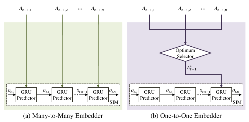
Figure 3: (a) The schematic diagrams of the Many-to-Many embedding method. (b) The schematic diagrams of the One-to-One embedding method.

Apart from the encoding and alignment, the most critical aspect of the SplatFlow framework is the embedding method of the temporal information into the two-frame backbone network. The red part in Fig. 1 shows the schematic diagram of the proposed One-to-Many embedding method. The method includes two keywords, “One” and “Many”.

As for the keyword “One”, we select the optimal aligned temporal information feature $A^{*}_{t-1}$ based on specific rules to be embedded into the two-frame backbone network. The only, same, and optimal additional input ensures that every iteration has a unified motion reference, reducing the ambiguity of early iterations, which is more conducive to the stability and convergence of the estimation result. In SplatFlow, we empirically take $A_{t-1,n}$ generated from the last iteration in the previous frame’s OFE process as $A^{*}_{t-1}$. The reason for choosing this selection rule is that the estimation error of the last iteration is the lowest. In addition, this brings the speed advantage that only the aligned temporal information of the last iteration needs to be calculated instead of all iterations.

In order to verify the advantages of the keyword “One”, we designed the Many-to-Many embedding method baseline, whose schematic diagram is shown in Fig. 3 (a). The Many-to-Many embedding method baseline removes the Optimum Selector module and instead uses the number of iterations as the selection basis to embed the different features in sequence $S=\{A_{t-1,1},A_{t-1,2},...,A_{t-1,n}\}$ into the different GRU iterations of the frame $t$. Similar to the multi-frame method for pyramid backbones, this method is designed for information interaction within the same layer/iteration, which is not conducive to fully utilizing the unique “single-resolution” characteristic of the advanced single-resolution iterative network.

The keyword “Many” is reflected in that every iteration will have the temporal information as an additional input, without exception. The advantage of this is that it makes the temporal information deeply participate in the network estimation process and can meet the different needs of different iteration contexts for using the temporal information.

In order to verify the advantages of the keyword “Many”, we designed the One-to-One embedding method baseline, whose schematic diagram is shown in Fig. 3 (b). In the One-to-One embedding method baseline, $A^{*}_{t-1}$ is obtained from sequence $S=\{A_{t-1,1},A_{t-1,2},...,A_{t-1,n}\}$ through the Optimum Selector module and is directly embedded in the last GRU iteration of the frame $t$. The embedding method is designed from the perspective of flow post-processing, so it is a backbone-independent multi-frame method, which has the advantages of more flexibility and easy implementation.

The comparisons between the proposed One-to-Many embedding method and the above two baselines are shown in Section 4.2.

The last concern is how to use the optimal aligned temporal information feature $A^{*}_{t-1}$ to guide each iteration during the current frame’s OFE. In the original GRU Predictor network, the input of the GRU Unit is the concatenation of the context feature $F^{c}_{t}$ and dynamically updated joint motion feature. In contrast, we concatenate $A^{*}_{t-1}$ with the above two features as a new input of GRU Unit in the proposed One-to-Many embedding method.

As described in GMA Jiang et al. (2021a), the concatenation operation allows the network to intelligently select from or combine the three features without prescribing exactly how it is to do this. In the case of occlusions, the network will refer to the temporal information feature when the optical flow cannot be inferred according to the current context.

3.4 Training and Inference

During training, our method uses three consecutive frames as a data unit and the flows of the previous two frames to supervise the network’s outputs. Specifically, we supervise our network on the $l_{1}$ distance between the predicted and the ground truth flow over the full sequences of the previous two frames’ predictions, $\{f_{(t-1,1)},...,f_{(t-1,n)}\}$ and $\{f_{(t,1)},...,f_{(t,n)}\}$, with exponentially increasing weights. Given the ground truth flow $g_{t-1}$ and $g_{t}$, the loss is defined as

$$L =L_{t-1}+L_{t}$$ (15)

$$=\sum_{i=1}^{n}\gamma^{i-n}||g_{t-1}-f_{t-1,i}||_{1}+\sum_{i=1}^{n}\gamma^{i-n}||g_{t}-f_{t,i}||_{1},$$ (16)

where we set $\gamma=0.85$ in our experiments. It is worth noting that since the data of KITTI Menze and Geiger (2015) does not have the ground truth of the first frame, i.e., $g_{t-1}$, we use Eq. (17) to calculate their losses:

$$L=L_{t}=\sum_{i=1}^{n}\gamma^{i-n}||g_{t}-f_{t,i}||_{1}.$$ (17)

When inferring the image sequence, the network calculates the optimal aligned temporal information feature $A^{*}$ for each frame except for the sequence’s first frame and embeds $A^{*}$ to the next frame’s estimation process under the proposed SplatFlow Framework. As for the inference of the first frame, it is consistent with the original two-frame backbone’s. That is, we directly reserve the two-frame backbone’s GRU Predictor network for inferring the first frame of an image sequence.

4 Experiments

Table 1: The statistical results of the overall, two-frame and multi-frame versions of the mainstream public optical flow datasets. Here only the left camera and clean pass are considered for Things Mayer et al. (2016), and only clean pass is considered for Sintel Butler et al. (2012).

Dataset	Max. Resolution	Training Scenes Number	Testing Scenes Number	Average Scene Length	Two-frame Training Units Number	Multi-frame Training Units Number	Two-frame Testing Units Number	Multi-frame Testing Units Number
Chairs Dosovitskiy et al. (2015)	512$\times$384	22232	640	2	22232	0	640	0
Things Mayer et al. (2016)	960$\times$540	2239	437	10	40302	35824	874	874
Sintel Butler et al. (2012)	1024$\times$436	23	12	46.51	1041	1018	552	552
KITTI Menze and Geiger (2015)	1240$\times$380	200	200	21	200	200	200	200
HD1K Kondermann et al. (2016)	2560$\times$1080	36	0	30.08	1047	1011	0	0

4.1 Datasets and Experimental Setup

4.1.1 Datasets

Mainstream public optical flow datasets include FlyingChairs Dosovitskiy et al. (2015), FlyingThings3D Mayer et al. (2016), Sintel Butler et al. (2012), KITTI2015 Menze and Geiger (2015) and HD1K Kondermann et al. (2016), etc. Among them, except for FlyingChairs Dosovitskiy et al. (2015), other datasets all include video sequences with frames equal to or more than 3. Our method needs to obtain useful information from the historical frames, and the data unit composed of three consecutive frames is used as input during training. Therefore, we adjust several mainstream datasets containing consecutive frames to serve as training datasets in our experiments. Table 1 shows the statistical results of the overall, two-frame, and multi-frame versions of the mainstream public optical flow datasets.

FlyingChairs Dosovitskiy et al. (2015)

This paper calls it Chairs for short. This is a synthetic dataset of moving 2D chair images superimposed on natural background images. It contains 22232 and 640 two-frame image pairs for training and testing, and there is no temporal link between them. Therefore, it can not build multi-frame datasets for the training and testing of our method.

FlyingThings3D Mayer et al. (2016)

This paper calls it Things for short. This is a synthetic dataset that relies on randomness and a large pool of rendering assets to generate orders of magnitude more data than the previous options. It contains 2239 training sequences and 437 testing sequences. Each sequence consists of 10 consecutive clean pass images. Therefore, each sequence can provide 9 two-frame image pairs. When only the left camera and clean pass are considered, the entire dataset can provide 40302 two-frame image pairs. When constructing a multi-frame dataset, we take 8 data units composed of three consecutive frames from each sequence. At this time, the total number of training data units is 35824. In addition, we take the middle two and three frames from each testing sequence to form a two-frame and multi-frame testing datasets containing 874 data units.

Sintel Butler et al. (2012)

This is a synthetic dataset that derives from an open-source 3D animated short film, and it has important features such as long sequences, large motions, specular reflections, motion blur, defocus blur, atmospheric effects, and so on. It contains 23 training sequences and 12 testing sequences. Most sequences are 50 frames long with 49 ground truths. This also reflects the original intention of the dataset design, that is, to encourage the development of methods that use longer sequences and integrate information over time. If only considering clean pass, there are 1041 two-frame image pairs for training a two-frame network. By collecting data units of three consecutive frames, we obtained a multi-frame training dataset containing 1018 data units. As for the testing dataset, we maintain the same number, i.e., 552, of units as the official, but except that the first unit of each sequence only includes two frames, the other units are all three frames.

KITTI2015 Menze and Geiger (2015)

This paper calls it KITTI for short. This is a realistic dataset obtained by annotating 400 dynamic scenes from the KITTI raw data collection using detailed 3D CAD models for all vehicles in motion. Two adjacent frames containing the expensive ground truth are selected from each scene to form a training dataset and a testing dataset with 200 two-frame data units each. We recall the previous frame of each frame containing the ground truth from the KITTI raw data collection and construct a new training dataset and testing dataset with the unchanged number of data units. It is more challenging than KITTI2012 Geiger et al. (2012) for the OFE task, which only contains static scenes.

HD1K Kondermann et al. (2016)

This is a realistic dataset that comprises a large number of difficult light and weather situations, such as low light, lens flares, rain, and wet streets. It contains 36 sequences and 1083 frames in total. Therefore, we can build a two-frame training dataset containing 1047 image pairs or a multi-frame training dataset containing 1011 data units based on it. Consistent with the previous method Teed and Deng (2020); Jiang et al. (2021a), we did not divide the testing dataset separately.

4.1.2 Evaluation Metrics

Table 2: Quantitative results of ablation experiments. All data come from C+T training process. The data marked with parentheses under the “Parameters” column indicates the model parameter amount used to infer non-first video frames.

Experiment	Variations	Things Mayer et al. (2016)		Sintel Butler et al. (2012)		KITTI Menze and Geiger (2015)		FPS	Parameters
		val		train		train
		Clean	Final	Clean	Final	EPE	Fl-all
GMA Jiang et al. (2021a)	-	4.98	4.23	1.31	2.75	4.48	16.9	12.96	5.9M
Alignment Method	Backward Flow	3.27	3.28	1.22	2.76	4.30	16.1	6.40	9.0M/(6.3M)
	Backward Warp	3.23	3.96	1.31	2.98	3.82	15.1	6.35	9.0M/(6.3M)
	Forward Warp	3.02	3.23	1.22	2.97	3.70	14.9	12.29	9.0M/(6.3M)
Differentiability	Non-differentiable Nearest	4.11	4.62	1.27	3.15	4.56	17.0	12.29	9.0M/(6.3M)
	Non-differentiable Splatting	3.25	3.44	1.26	3.05	3.98	15.9	12.29	9.0M/(6.3M)
	Differentiable Splatting	3.02	3.23	1.22	2.97	3.70	14.9	12.29	9.0M/(6.3M)
Splatting Type	Softmax Splatting	2.97	3.30	1.20	2.97	3.92	15.2	11.97	9.0M/(6.3M)
	Average Splatting	3.02	3.23	1.22	2.97	3.70	14.9	12.29	9.0M/(6.3M)
Embedding Method	One-to-One	3.49	4.09	1.37	3.10	4.19	16.2	12.51	9.0M/(6.3M)
	Many-to-Many	3.45	3.43	1.27	3.10	4.20	16.2	10.56	9.0M/(6.3M)
	One-to-Many	3.02	3.23	1.22	2.97	3.70	14.9	12.29	9.0M/(6.3M)

Commonly used metrics in OFE include the end-point error (EPE) and the percentage of optical flow outliers (Fl).

Depending on the scope of the evaluation, EPE can be further divided into EPE-all (EPE), EPE-noc and EPE-occ, which are used to evaluate the average pixel end-point error over all, non-occluded, and occluded ground truth pixel regions, respectively.

Fl can be further divided into Fl-all, Fl-bg, and Fl-fg, which are used to evaluate the percentage of outliers averaged over all, background and foreground ground truth pixel regions, respectively. It is worth noting that the metric Fl is mainly used to evaluate on KITTI Menze and Geiger (2015) benchmark. The benchmark considers a pixel to be correctly estimated if the flow end-point error is <3px or <5%.

4.1.3 Implemental Details

We use PyTorch to implement our method, and the two-frame backbone network of our final version is GMA Jiang et al. (2021a). Compared with RAFT Teed and Deng (2020), GMA Jiang et al. (2021a) will additionally input the current frame’s aggregated global joint motion feature calculated through the attention mechanism at each GRU iteration. We use average splatting as our differentiable forward warping transformation. We are consistent with GMA Jiang et al. (2021a) in training and inference hyperparameters, including the number of GRU iterations, the AdamW Loshchilov and Hutter (2017) as an optimizer, and the One-cycle Smith and Topin (2019) as the learning rate adjustment strategy. We use the TITAN RTX GPU for training and inference. Unless otherwise noted, we evaluate after 24 flow iterations on Things Mayer et al. (2016) and KITTI Menze and Geiger (2015), and 32 on Sintel Butler et al. (2012).

4.1.4 Training Processes

Our training process includes three parts, namely C+T, S-finetune, and K-finetune. They are the inheritances of GMA Jiang et al. (2021a)’s training processes and make some adjustments.

C+T

The training datasets of this process in GMA Jiang et al. (2021a) are Chairs Dosovitskiy et al. (2015) and Things Mayer et al. (2016). In contrast, we only use Things Mayer et al. (2016), but the training is divided into two stages. The first stage is to load and freeze GMA Jiang et al. (2021a)’s pre-training weights on C+T, and separately train the GRU Predictor and Convex Upsampling networks’ parameters. The second step is to release all frozen parameters and then finetune all of the parameters. The batch size in both steps is 8, the learning rate is all $1.25\times 10^{-4}$, and the number of training steps is all 100K.

S-finetune

In this process, we finetune the model obtained by C+T on a mixed dataset dominated by Sintel Butler et al. (2012) composed of four datasets, i.e., Things Mayer et al. (2016), Sintel Butler et al. (2012), KITTI Menze and Geiger (2015) and HD1K Kondermann et al. (2016). The batch size is 8, the learning rate is $1.25\times 10^{-4}$, and the number of training steps is 120K. We use the model of this process to be submitted and evaluate the testing dataset on Sintel Butler et al. (2012) benchmark.

K-finetune

In this process, we finetune the model obtained by S-finetune on a KITTI Menze and Geiger (2015) data-enhanced hybrid dataset composed of the same four datasets. The batch size is 6, the learning rate is $1.25\times 10^{-4}$, and the number of training steps is 50K. We use the model of this process to be submitted and evaluate the testing dataset on KITTI Menze and Geiger (2015) benchmark.

4.2 Ablation Studies

We conduct a series of ablation experiments on our method from five aspects, which include alignment method, differentiability of transformation, splatting type, embedding method, and the number of iterations, to examine their contributions. In all experiments, we use the model after C+T training process and evaluate each model on Things test Mayer et al. (2016), Sintel train Butler et al. (2012), and KITTI train Menze and Geiger (2015) datasets. All quantitative results are shown in Table 2, and the visualization results about the number of iterations are shown in Fig 4.

4.2.1 Temporal Information Alignment Method

We compare three temporal information alignment methods, denoted as “Backward Flow”, “Backward Warp”, and “Forward Warp”. Different from the other two methods, “Backward Flow” baseline directly takes the backward JMF in the backward flow estimation process from the frame $t$ to the frame $t-1$ as the aligned temporal information. ‘Backward Warp’ baseline uses the backward flow to bi-linear sample the forward JMF of the frame $t-1$, so as to achieve feature alignment. “Forward Warp” refers to the proposed method.

The “Alignment Method” part of Table 2 shows the quantitative results of the three methods. It can be seen from the results that our method achieves the best performance in 5 of 6 dataset metrics over the other two baselines, which proves the effectiveness of the forward warping transformation in aligning the temporal information. Since there is no need to calculate the backward flow, the inference speed of the proposed method is nearly twice that of the other two baselines. Notably, the inference speed of “Backward Flow” and “Backward Warp” is very close, which also illustrates that the time consumption of the backward warping transformation is essentially negligible compared to calculating the backward flow.

4.2.2 Differentiability of Forward Warping Transformation

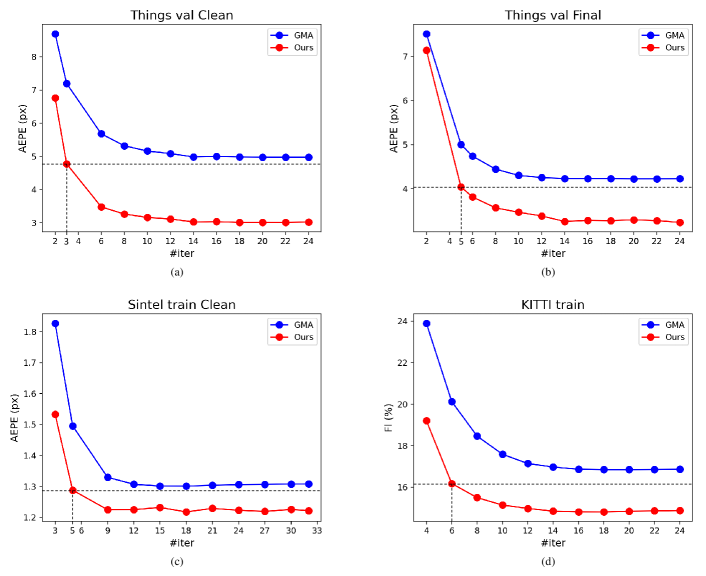
Figure 4: Datasets evaluation results vs. the number of iterations at inference time. As single-resolution iterative methods, our method and GMA Jiang et al. (2021a) both quickly converge, comparable with final results only after 12 iterations. Our method surpasses GMA Jiang et al. (2021a)’s final performance only after less than five average iterations.

Table 3: Quantitative results of comparisons between the proposed method and two-frame backbone networks. All data come from C+T training process. The data marked with parentheses under the “Parameters” column indicates the model parameter amount used for inferring non-first video frames.

Backbone	Multi-frame Settings	Things Mayer et al. (2016)		Sintel Butler et al. (2012)		KITTI Menze and Geiger (2015)		FPS	Parameters
		val		train		train
		Clean	Final	Clean	Final	EPE	Fl-all
RAFT Teed and Deng (2020)	No	5.24	4.74	1.46	2.70	5.03	17.5	17.06	5.3M
	Yes (SplatFlow-RAFT)	3.43	3.29	1.24	2.84	4.55	16.2	15.35	8.0M/(5.7M)
GMA Jiang et al. (2021a)	No	4.98	4.23	1.31	2.75	4.48	16.9	12.96	5.9M
	Yes (SplatFlow-GMA)	3.02	3.23	1.22	2.97	3.70	14.9	12.29	9.0M/(6.3M)

Here we analyze the impact of forward warping transformation’s differentiability on performance. We design two types of non-differentiable forward warping transformation, i.e., “Non-differentiable Nearest” and “Non-differentiable Splatting”. “Non-differentiable Nearest” baseline fills the temporal information to the nearest integer pixel of the target sub-pixel position. “Non-differentiable Splatting” is constructed by directly disabling the gradient propagation of our method’s splatting transformation during training. From the “Differentiability” part of Table 2, we find that our proposed “Differentiable Splatting” is better than “Non-differentiable Splatting”, and “Non-differentiable Splatting” is better than “Non-differentiable Nearest” in all dataset metrics. It shows that both the differentiability and sub-pixel level filling has the effect of improving the performance of forward warping transformation on OFE.

4.2.3 Splatting Type

We design the “Softmax Splatting” baseline according to Eq. (12) to observe the impact of splatting type on the estimation effect. Correspondingly, “Average Splatting” is our proposed method, which is based on Eq. (11). The “Splatting Type” part of Table 2 shows the quantitative results of the two methods.

Compared with “Softmax Splatting”, “Average Splatting” can achieve considerable or even better results with the best performance in 4 of 6 dataset metrics, which shows that the average splatting can be better generalized to more scenes in OFE tasks. We find that “Softmax Splatting” has a weak advantage over “Average Splatting” in Things val Mayer et al. (2016) Clean and Sintel train Butler et al. (2012) Clean datasets. We think that compared with realistic and final pass data, the texture of clean pass data is simpler, and it is easier to extract more discriminative image feature representation, which is conducive to softmax splatting playing its theoretical advantages in eliminating mapping conflicts. In addition, because there is no need to calculate the feature similarity and its exponential value between source and target pixels, “Average Splatting” also has a faster inference speed.

4.2.4 Temporal Information Embedding Method

According to the characteristics of the single-resolution iterative two-frame backbone networks, we designed a One-to-Many embedding method. In order to prove the effectiveness of the proposed embedding method, we also designed two intuitively reasonable baselines, i.e., the “Many-to-Many” and the “One-to-One” embedding methods. Fig. 1’s red part and Fig. 3 show the structural differences between the three methods.

From the “Embedding Method” part of Table 2, we can see that the proposed “One-to-Many” embedding method is better than the “One-to-One” and the “Many-to-Many” methods in all dataset metrics. It proves that taking the optimal temporal information as a unified motion reference to participate deeply in the network estimation process can maximize the guiding effect of the multi-frame temporal information. At the same time, the inference speed of the “One-to-Many” embedding method is comparable to that of the “One-to-One”, which shows that the time consumption of the temporal information as an additional input to the GRU Unit is minimal. In addition, the obvious speed advantage of the “One-to-Many” embedding method over the “Many-to-Many” comes from the optimum selection rule that only calculates the aligned temporal information for the final rather than every iteration.

4.2.5 Number of Iterations

In order to make a fair comparison with the previous methods, we adopt a large number of iterations for inference when evaluating the datasets (24 for Things Mayer et al. (2016) and KITTI Menze and Geiger (2015), 32 for Sintel Butler et al. (2012)). In fact, similar to other single-resolution iterative methods, our method quickly converges, comparable with final results only after 12 iterations, which can be seen in Fig 4. It is worth noting that our method surpasses GMA Jiang et al. (2021a)’s final performance only after less than five average iterations. At this point, if we compare the final time consumed by GMA Jiang et al. (2021a) on Sintel Butler et al. (2012) (32 iterations), we can get a $4.01\times$ increase in speed, i.e., 5.61 fps vs. 22.49 fps on the TITAN RTX GPU.

This experiment shows that the proposed method is highly adapted to the “iterative” characteristic of backbones and has great advantages in performance.

4.3 Comparisons with Two-frame Backbone

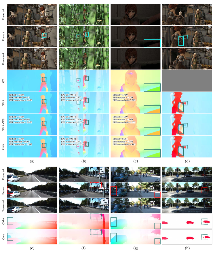
Figure 5: Qualitative results of GMA Jiang et al. (2021a) and our method on Sintel Butler et al. (2012) test Clean ((a)-(d)) and KITTI2015 Menze and Geiger (2015) test ((e)-(h)) datasets. The “GMA+WS” row in (a)-(d) shows the qualitative results of WarmStart Teed and Deng (2020) method on Sintel Butler et al. (2012) test Clean dataset. The (a)-(c) columns are examples, including the ground truths and evaluation values reported on Sintel benchmark. On the contrary, the ground truth of (d) is unavailable and is replaced by gray. The solid-box marked regions are significantly occluded in the frame $t+1$, and the dotted-box marked regions are non-occluded but challenging to estimate. The contents of the boxes show that our method can get more detailed results in non-occluded regions while more acceptable performance in occluded regions.

Table 4: The evaluation results and relative improvements compared the proposed methods with their two-frame backbones on three types of regions (non-occluded, occluded, and all).

Training Process	Dataset	Region Type	RAFT Teed and Deng (2020)	SplatFlow -RAFT	Rel. Impr. on RAFT (%)	GMA Jiang et al. (2021a)	SplatFlow -GMA	Rel. Impr. on GMA (%)
C+T	Things Mayer et al. (2016) val Clean	Noc	1.88	1.43	23.9	1.96	1.32	32.7
		Occ	16.62	8.85	46.8	15.59	8.05	48.4
		All	5.24	3.43	34.5	4.98	3.02	39.4
	Things Mayer et al. (2016) val Final	Noc	1.72	1.45	15.7	1.71	1.53	10.5
		Occ	14.90	8.27	44.5	13.41	8.24	38.6
		All	4.74	3.29	30.6	4.23	3.23	23.6
	Sintel Butler et al. (2012) train Clean	Noc	0.64	0.61	4.7	0.59	0.59	0.0
		Occ	11.81	9.24	21.8	10.49	9.23	12.0
		All	1.46	1.24	15.1	1.31	1.22	6.9
Sintel-finetune	Sintel Butler et al. (2012) train Clean	Noc	0.33	0.28	15.2	0.29	0.26	10.3
		Occ	6.23	4.24	31.9	4.96	4.00	19.4
		All	0.76	0.57	25.0	0.63	0.53	15.9
	Sintel Butler et al. (2012) train Final	Noc	0.67	0.54	19.4	0.58	0.53	8.6
		Occ	8.13	6.10	25.0	7.04	5.74	18.5
		All	1.22	0.94	23.0	1.05	0.91	13.3
	Sintel Butler et al. (2012) test Clean	Noc	0.76	0.51	32.9	0.56	0.51	8.9
		Occ	11.48	6.62	42.3	8.13	6.06	25.5
		All	1.93	1.18	38.9	1.39	1.12	19.4
	Sintel Butler et al. (2012) test Final	Noc	1.55	1.38	11.0	1.40	1.06	24.3
		Occ	16.46	12.85	21.9	14.96	10.29	31.2
		All	3.18	2.64	17.0	2.88	2.07	28.1

In this subsection, we compare the proposed method with the single-resolution backbone networks to show and analyze the role of introducing the temporal information.

Firstly, we take RAFT Teed and Deng (2020) and GMA Jiang et al. (2021a) as backbone networks, respectively. We show their quantitative results and multi-frame versions after C+T training process. As shown in Table 3, compared with the original backbone networks, after embedding the multi-frame temporal information guidance, the networks can achieve significant performance improvements in almost all dataset metrics. At the same time, due to the use of a unidirectional information aggregation method based on splatting transformation, the two multi-frame versions maintain similar inference speeds with their backbones. If we only consider inferring non-first video frames, the multi-frame versions also have comparable parameter amounts with their backbones.

It is worth noting that the “SplatFlow-GMA” baseline, i.e., our final model, as “RAFT” baseline integrating both the temporal and spatial information Jiang et al. (2021a), has significantly better performance than the “SplatFlow-RAFT” baseline or “GMA” baseline in Table 3. This shows that the temporal information and the spatial information are two kinds of complementary information, which can not be replaced by each other. Moreover, it further illustrates that the temporal information is indispensable to improving the accuracy of OFE. Besides, we find that the “SplatFlow-RAFT” baseline outperforms “GMA” baseline on inference speed and 4 of 6 dataset metrics, and even on parameter amount if only considering inferring non-first video frames. It shows that, in most cases, the temporal information is even more valuable than the spatial information.

Then, we further explore the impact of the temporal information on occlusions. Table 4 shows the evaluation results and relative improvements compared “SplatFlow-RAFT” and “SplatFlow-GMA” baselines with their two-frame backbones RAFT Teed and Deng (2020) and GMA Jiang et al. (2021a) on three types of regions (non-occluded, occluded, and all) on Things Mayer et al. (2016) val and Sintel Butler et al. (2012) train Clean datasets after C+T training process and on Sintel train and Sintel test datasets after S-finetune training process. Considering that KITTI Menze and Geiger (2015) dataset has no ground truth of occluded regions, we did not evaluate it. We find that our methods achieve performance improvements in all three regions of all datasets after all training processes. Among them, the improvements in occluded regions are the most significant, without exception. These show that the network can benefit from embedding the temporal information in every region, especially in occluded regions.

Fig. 5 shows the qualitative results of our method and GMA on Sintel test Clean after S-finetune and KITTI test after K-finetune training processes. The solid-box marked regions are significantly occluded in the frame $t+1$, and the dotted-box marked regions are non-occluded but challenging to estimate. The contents of the boxes show that our method can get more detailed results in non-occluded regions while more acceptable performance in occluded regions, avoiding the large area of failure. Meanwhile, the evaluation values reported on Sintel benchmark in Fig. 5 (a)-(b) show that our method has indeed surpassed GMA in all three regions, which is consistent with the conclusion in Table 4.

The above results show that the proposed method effectively uses the temporal information to comprehensively optimize the effect of OFE.

4.4 Comparisons with Multi-frame Baselines

Table 5: Quantitative results of comparisons among multi-frame methods. All data come from C+T training process. The data marked with parentheses under the “Parameters” column indicates the model parameter amount used for inferring non-first video frames.

Backbone	Multi-frame Method	Things Mayer et al. (2016)		Sintel Butler et al. (2012)		KITTI Menze and Geiger (2015)		FPS	Parameters
		val		train		train
		Clean	Final	Clean	Final	EPE	Fl-all
RAFT Teed and Deng (2020)	-	5.24	4.74	1.46	2.70	5.03	17.5	17.06	5.3M
	FusionFlow Ren et al. (2019)	4.82	5.11	1.36	2.97	4.89	17.7	4.87	5.8M
	WarmStart Teed and Deng (2020)	4.96	4.64	1.42	2.70	4.92	17.5	13.10	5.3M
	SplatFlow (Ours)	3.43	3.29	1.24	2.84	4.55	16.2	15.35	8.0M/(5.7M)
GMA Jiang et al. (2021a)	-	4.98	4.23	1.31	2.75	4.48	16.9	12.96	5.9M
	FusionFlow Ren et al. (2019)	4.60	5.02	1.29	3.16	4.47	16.8	4.16	6.4M
	WarmStart Teed and Deng (2020)	5.16	4.24	1.30	2.71	4.48	16.9	10.61	5.9M
	SplatFlow (Ours)	3.02	3.23	1.22	2.97	3.70	14.9	12.29	9.0M/(6.3M)

Table 6: Quantitative results on Sintel Butler et al. (2012) and KITTI Menze and Geiger (2015) benchmarks. The best result of each metric is marked in bold. The evaluation result on the training dataset of the training process is marked in parentheses, and the evaluation result on the testing dataset is not marked in parentheses. * indicates the result with the WarmStart Teed and Deng (2020) initialization method of single-resolution iterative networks.

Training Data	Method	Sintel Butler et al. (2012) train		KITTI Menze and Geiger (2015) train		Sintel Butler et al. (2012) test		KITTI Menze and Geiger (2015) test
		Clean	Final	AEPE	F1-all	Clean	Final	Fl-all
C+T	LiteFlowNet2 Hui et al. (2020)	2.24	3.78	8.97	25.9	-	-	-
	VCN Yang and Ramanan (2019)	2.21	3.68	8.36	25.1	-	-	-
	MaskFlowNet Zhao et al. (2020)	2.25	3.61	-	23.1	-	-	-
	FlowNet2 Ilg et al. (2017)	2.02	3.54	10.08	30	3.96	6.02	-
	DICL Wang et al. (2020)	1.94	3.77	8.7	23.6	-	-	-
	RAFT Teed and Deng (2020)	1.43	2.71	5.04	17.4	-	-	-
	SeparableFlow Zhang et al. (2021)	1.30	2.59	4.60	15.9	-	-	-
	GMA Jiang et al. (2021a)	1.30	2.74	4.69	17.1	-	-	-
	Ours	1.22	2.97	3.70	14.9	-	-	-
S-finetune	FlowNet2 Ilg et al. (2017)	(1.45)	(2.01)	-	-	4.16	5.74	-
	PWC-Net+ Sun et al. (2019)	(1.71)	(2.34)	-	-	3.45	4.60	-
	LiteFlowNet2 Hui et al. (2020)	(1.30)	(1.62)	-	-	3.48	4.69	-
	HD3 Yin et al. (2019)	(1.87)	(1.17)	-	-	4.79	4.67	-
	IRR-PWC Hur and Roth (2019)	(1.92)	(2.51)	-	-	3.84	4.58	-
	VCN Yang and Ramanan (2019)	(1.66)	(2.24)	-	-	2.81	4.40	-
	MaskFlowNet Zhao et al. (2020)	-	-	-	-	2.52	4.17	-
	ScopeFlow Bar-Haim and Wolf (2020)	-	-	-	-	3.59	4.10	-
	DICL Wang et al. (2020)	(1.11)	(1.60)	-	-	2.12	3.44	-
	RAFT Teed and Deng (2020)	(0.76)	(1.22)	-	-	1.61*	2.86*	-
	SeparableFlow Zhang et al. (2021)	(0.69)	(1.10)	-	-	1.50	2.67	-
	GMA Jiang et al. (2021a)	(0.62)	(1.06)	-	-	1.39*	2.47*	-
	Ours	(0.53)	(0.91)	-	-	1.12	2.07	-
K-finetune	FlowNet2 Ilg et al. (2017)	-	-	(2.30)	(6.8)	-	-	11.48
	PWC-Net+ Sun et al. (2019)	-	-	(1.50)	(5.3)	-	-	7.72
	LiteFlowNet2 Hui et al. (2020)	-	-	(1.47)	(4.8)	-	-	7.74
	HD3 Yin et al. (2019)	-	-	(1.31)	(4.1)	-	-	6.55
	IRR-PWC Hur and Roth (2019)	-	-	(1.63)	(5.3)	-	-	7.65
	VCN Yang and Ramanan (2019)	-	-	(1.16)	(4.1)	-	-	6.30
	MaskFlowNet Zhao et al. (2020)	-	-	-	-	-	-	6.10
	ScopeFlow Bar-Haim and Wolf (2020)	-	-	-	-	-	-	6.82
	DICL Wang et al. (2020)	-	-	(1.02)	(3.6)	-	-	6.31
	RAFT Teed and Deng (2020)	-	-	(0.63)	(1.5)	-	-	5.10
	SeparableFlow Zhang et al. (2021)	-	-	(0.69)	(1.6)	-	-	4.64
	GMA Jiang et al. (2021a)	-	-	(0.57)	(1.2)	-	-	5.15
	Ours	-	-	(0.80)	(2.4)	-	-	4.61

Table 7: The Quantitative results of comparisons between the proposed method and its backbone GMA Jiang et al. (2021a) after C+T training process on Sintel Butler et al. (2012) train Final dataset sequence by sequence. The “Error Increment” row only displays an error increment whose value is a positive number. The biggest error increment is marked in bold.

Scene Name	alley_1	alley_2	ambush_2	ambush_4	ambush_5	ambush_6	ambush_7	bamboo_1
GMA	0.21	0.20	20.44	14.63	6.98	7.42	0.52	0.38
Ours	0.21	0.17	20.70	21.94	8.20	8.12	0.38	0.36
Error Increment	0.00	-	0.26	7.31	1.22	0.70	-	-
Scene Name	bamboo_2	bandage_1	bandage_2	cave_2	cave_4	market_2	market_5	market_6
GMA	0.78	0.42	0.46	5.81	3.15	0.60	9.03	2.34
Ours	0.66	0.40	0.46	5.10	3.15	0.63	8.88	1.87
Error Increment	-	-	0.00	-	-	0.03	-	-
Scene Name	mountain_1	shaman_2	shaman_3	sleeping_1	sleeping_2	temple_2	temple_3
GMA	0.26	0.26	0.24	0.12	0.11	2.33	4.01
Ours	0.28	0.25	0.22	0.11	0.09	1.84	4.34
Error Increment	0.02	-	-	-	-	-	0.33

In this subsection, we compare the proposed method with other multi-frame methods based on single-resolution iterative backbone networks to show and analyze the advantages of our method.

The multi-frame method is divided into backbone-dependent and backbone-independent. The existing multi-frame methods, such as SelFlow Liu et al. (2019) and ContinualFlow Neoral et al. (2018), are mainly backbone-dependent and based on pyramid backbones like PWC-Net Sun et al. (2018). We use the initialization method called WarmStart proposed in RAFT Teed and Deng (2020) as a backbone-dependent multi-frame baseline based on single-resolution iterative backbones. In addition, we choose FlowFusion Ren et al. (2019), which has achieved good results on PWC-Net Sun et al. (2018), as the backbone-independent multi-frame baseline. We use three methods on RAFT Teed and Deng (2020) and GMA Jiang et al. (2021a) backbones, and quantitative results are shown in Table 5.

First, we find our method is superior to FlowFusion Ren et al. (2019) in all dataset metrics, no matter which backbone is based on. It shows that making full use of the characteristics of the backbone network could achieve better estimation performance. Besides, we found that our inference speeds are nearly $3\times$ that of FlowFusion Ren et al. (2019)’s. The speed advantage is mainly attributed to the fact that the splatting transformation can transmit the temporal information continuously in one direction, thus avoiding the time consumption of computing the backward flow. If we only consider inferring non-first video frames, our methods would have fewer parameter amounts than FlowFusion Ren et al. (2019).

Second, compared with WarmStart Teed and Deng (2020), our methods achieve the best performance in 5 of 6 dataset metrics. It shows that our method can make more effective use of the multi-frame temporal information to improve performance. The “GMA+WS” row in Fig. 5 (a)-(d) shows the qualitative results of WarmStart Teed and Deng (2020) method on Sintel Butler et al. (2012) test Clean dataset. It can be seen from Fig. 5 that although “GMA+WS” has made slight improvement compared with “GMA”, it still cannot cope with the challenging occlusion problems correctly. Even in many cases, the performance of “GMA+WS” is unchanged or decreased compared with that of the backbone, which is also reflected in the performance of “GMA+WarmStart” on Things Mayer et al. (2016) val dataset in Table 5. As for inference speed, the “forward_interpolate” operation used in WarmStart Teed and Deng (2020) is on the CPU and therefore takes longer.

To sum up, the above experiments fully demonstrate that our method has comprehensive and significant advantages in multi-frame information utilization, taking speed and accuracy into account simultaneously.

4.5 Results on Benchmarks

We evaluate our method on public Sintel Butler et al. (2012) and KITTI Menze and Geiger (2015) benchmarks and compare the results against prior works; the results are shown in Table 6.

Firstly, after C+T training process (first part in Table 6), we significantly exceed all the existing methods on most of the metrics on Sintel Butler et al. (2012) train and KITTI Menze and Geiger (2015) train datasets, demonstrating our method’s superior cross-dataset generalization performance.

Secondly, after S-finetune training process (second part in Table 6), our method ranks first on both Sintel Butler et al. (2012) test Clean and Sintel Butler et al. (2012) test Final datasets, with EPEs of 1.12 and 2.07, a 19.4% and 16.2 % error decrease over the previous best method GMA Jiang et al. (2021a). At the same time, our method also achieves the lowest error on Sintel Butler et al. (2012) train Clean and Final datasets, which are the components of the training datasets during S-finetune process. It proves that our method can dig and use useful clues at a deeper level, thus achieving a better training convergence effect.

Finally, after K-finetune training process (third part in Table 6), our method ranks first among all methods based on optical flow on KITTI Menze and Geiger (2015) test dataset. It is worth noting that our performance on the training datasets of this process is not outstanding. It is because we reduced the proportion of KITTI Menze and Geiger (2015) data compared with other methods during training. The reason for the reduction is to prevent overfitting KITTI Menze and Geiger (2015) train dataset, which only has a small amount of data.

These three sets of results show that our method has a higher generalization performance than the previous best method and has reached a new state-of-the-art performance on two public benchmarks, proving its effectiveness and advancement.

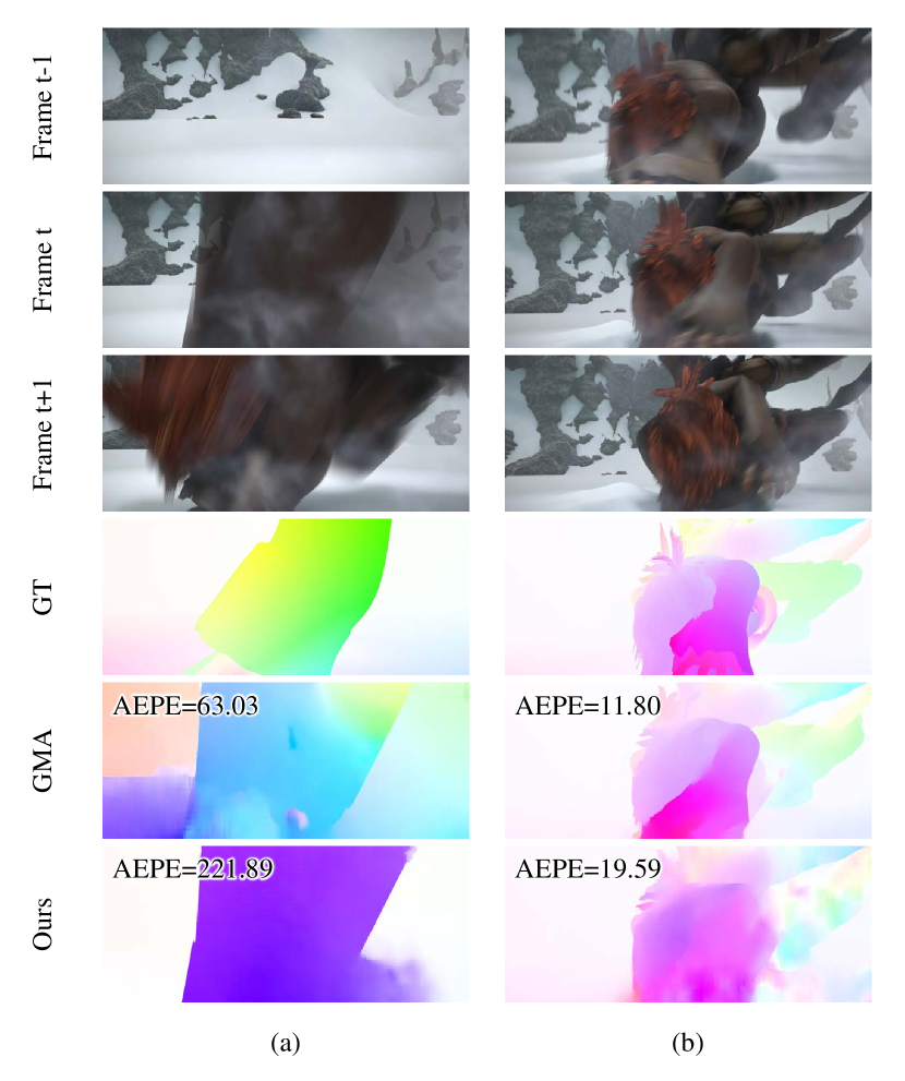
Figure 6: Example Qualitative results of two cases in which our method has large errors on the “ambush_4” sequence of Sintel Butler et al. (2012) train Final dataset. In the first case (a), the image is seriously blurred, and the motion displacement is huge, which can not be judged even by human eyes. In the other case (b), the image has large blurs, which are not found during training.

4.6 Discussion

In this subsection, we explore why the proposed methods perform slightly worse than their backbones on Sintel Butler et al. (2012) train Final dataset in Table 3. Considering that the appearances and motion distributions of objects in the same video sequence are similar, we evaluate the two methods sequence by sequence on Sintel Butler et al. (2012) train Final dataset to find video sequences that are difficult to evaluate. Table 7 shows the quantitative results.

As can be seen from Table 7, there are 23 video sequences in total. Among them, the error increment of the “ambush_4” sequence is extremely large, while other sequences’ are negative or small enough to be ignored.

Through careful observation of the “ambush_4” sequence, we find that our method mainly has large errors in two cases, and their example qualitative results are shown in Fig 6. In the first case, the image is seriously blurred, and the motion displacement is huge, which can not be judged even by human eyes, as shown in Fig. 6 (a). In this case, both methods fail and produce great errors. Therefore the relative error is also large and random. In the other case, the image has large blurs, which are not found in Things Mayer et al. (2016) train dataset during C+T training process, as shown in Fig. 6 (b). In this case, our method will produce fog-like error estimation in fuzzy areas, which does not exist in Sintel Butler et al. (2012) test Final dataset after S-finetune training process. This shows that compared with GMA Jiang et al. (2021a), our method has poor generalization for fuzzy texture. This can be improved by using data enhancements that simulate blurring or by adding training samples with blurring.

5 Conclusion

In summary, we propose a MOFE framework named SplatFlow, which is realized by introducing the differentiable splatting transformation to align the temporal information, designing a One-to-Many embedding method to densely guide the current frame’s estimation, and further remodelling the existing two-frame backbones. The proposed SplatFlow framework has significant occlusion coping ability and balanced evaluation accuracy and speed.

Through this work, we further prove that the multi-frame settings play an active and indispensable role in solving occlusions and improving the accuracy of OFE. It will be a potential research direction to explore more effective multi-frame methods for mining and integrating the temporal information.

References

- Aslani and Mahdavi-Nasab (2013) Aslani S., Mahdavi-Nasab H. (2013) Optical flow based moving object detection and tracking for traffic surveillance. International Journal of Electrical, Computer, Energetic, Electronic and Communication Engineering 7(9):1252–1256
- Bailer et al. (2015) Bailer C., Taetz B., Stricker D. (2015) Flow fields: Dense correspondence fields for highly accurate large displacement optical flow estimation. In: ICCV, IEEE, pp. 4015–4023
- Bao et al. (2019) Bao W., Lai W.-S., Ma C., Zhang X., Gao Z., Yang M.-H. (2019) Depth-aware video frame interpolation. In: CVPR, IEEE, pp. 3703–3712
- Bar-Haim and Wolf (2020) Bar-Haim A., Wolf L. (2020) Scopeflow: Dynamic scene scoping for optical flow. In: CVPR, IEEE, pp. 7998–8007
- Brox et al. (2009) Brox T., Bregler C., Malik J. (2009) Large displacement optical flow. In: CVPR, IEEE, pp. 41–48
- Butler et al. (2012) Butler D. J., Wulff J., Stanley G. B., Black M. J. (2012) A naturalistic open source movie for optical flow evaluation. In: ECCV, Springer, pp. 611–625
- Caballero et al. (2017) Caballero J., Ledig C., Aitken A., Acosta A., Totz J., Wang Z., Shi W. (2017) Real-time video super-resolution with spatio-temporal networks and motion compensation. In: CVPR, IEEE, pp. 4778–4787
- Cheng et al. (2017) Cheng J., Tsai Y.-H., Wang S., Yang M.-H. (2017) Segflow: Joint learning for video object segmentation and optical flow. In: ICCV, IEEE, pp. 686–695
- Choi et al. (2014) Choi Y.-W., Kwon K.-K., Lee S.-I., Choi J.-W., Lee S.-G. (2014) Multi-robot mapping using omnidirectional-vision slam based on fisheye images. ETRI Journal 36(6):913–923
- Cun et al. (2018) Cun X., Xu F., Pun C.-M., Gao H. (2018) Depth-assisted full resolution network for single image-based view synthesis. IEEE computer graphics and applications 39(2):52–64
- Dosovitskiy et al. (2015) Dosovitskiy A., Fischer P., Ilg E., Hausser P., Hazirbas C., Golkov V., Van Der Smagt P., Cremers D., Brox T. (2015) Flownet: Learning optical flow with convolutional networks. In: ICCV, IEEE, pp. 2758–2766
- Gao et al. (2020) Gao C., Saraf A., Huang J.-B., Kopf J. (2020) Flow-edge guided video completion. In: ECCV, Springer, pp. 713–729
- Geiger et al. (2012) Geiger A., Lenz P., Urtasun R. (2012) Are we ready for autonomous driving? the kitti vision benchmark suite. In: CVPR, IEEE, pp. 3354–3361
- Gibson (1950) Gibson J. J. (1950) The perception of the visual world
- Godard et al. (2017) Godard C., Mac Aodha O., Brostow G. J. (2017) Unsupervised monocular depth estimation with left-right consistency. In: CVPR, IEEE, pp. 270–279
- Horn and Schunck (1981) Horn B. K., Schunck B. G. (1981) Determining optical flow. Artificial intelligence 17(1-3):185–203
- Hu et al. (2022) Hu P., Niklaus S., Sclaroff S., Saenko K. (2022) Many-to-many splatting for efficient video frame interpolation. In: CVPR, IEEE, pp. 3553–3562
- Hui et al. (2018) Hui T.-W., Tang X., Loy C. C. (2018) Liteflownet: A lightweight convolutional neural network for optical flow estimation. In: CVPR, IEEE, pp. 8981–8989
- Hui et al. (2020) Hui T.-W., Tang X., Loy C. C. (2020) A lightweight optical flow cnn—revisiting data fidelity and regularization. IEEE Transactions on Pattern Analysis and Machine Intelligence 43(8):2555–2569
- Hur and Roth (2019) Hur J., Roth S. (2019) Iterative residual refinement for joint optical flow and occlusion estimation. In: CVPR, IEEE, pp. 5754–5763
- Ilg et al. (2017) Ilg E., Mayer N., Saikia T., Keuper M., Dosovitskiy A., Brox T. (2017) Flownet 2.0: Evolution of optical flow estimation with deep networks. In: CVPR, IEEE, pp. 2462–2470
- Irani (1999) Irani M. (1999) Multi-frame optical flow estimation using subspace constraints. In: ICCV, IEEE, vol 1, pp. 626–633
- Jason et al. (2016) Jason J. Y., Harley A. W., Derpanis K. G. (2016) Back to basics: Unsupervised learning of optical flow via brightness constancy and motion smoothness. In: ECCV, Springer, pp. 3–10
- Jiang et al. (2018) Jiang H., Sun D., Jampani V., Yang M.-H., Learned-Miller E., Kautz J. (2018) Super slomo: High quality estimation of multiple intermediate frames for video interpolation. In: CVPR, IEEE, pp. 9000–9008
- Jiang et al. (2021a) Jiang S., Campbell D., Lu Y., Li H., Hartley R. (2021a) Learning to estimate hidden motions with global motion aggregation. In: ICCV, IEEE, pp. 9772–9781
- Jiang et al. (2021b) Jiang S., Lu Y., Li H., Hartley R. (2021b) Learning optical flow from a few matches. In: CVPR, pp. 16,592–16,600
- Jonschkowski et al. (2020) Jonschkowski R., Stone A., Barron J. T., Gordon A., Konolige K., Angelova A. (2020) What matters in unsupervised optical flow. In: ECCV, Springer, pp. 557–572
- Kondermann et al. (2016) Kondermann D., Nair R., Honauer K., Krispin K., Andrulis J., Brock A., Gussefeld B., Rahimimoghaddam M., Hofmann S., Brenner C., et al. (2016) The hci benchmark suite: Stereo and flow ground truth with uncertainties for urban autonomous driving. In: CVPR Workshops, IEEE, pp. 19–28
- Li et al. (2019) Li Z., Dekel T., Cole F., Tucker R., Snavely N., Liu C., Freeman W. T. (2019) Learning the depths of moving people by watching frozen people. In: CVPR, IEEE, pp. 4521–4530
- Liu et al. (2018) Liu M., He X., Salzmann M. (2018) Geometry-aware deep network for single-image novel view synthesis. In: CVPR, IEEE, pp. 4616–4624
- Liu et al. (2019) Liu P., Lyu M., King I., Xu J. (2019) Selflow: Self-supervised learning of optical flow. In: CVPR, IEEE, pp. 4571–4580
- Loshchilov and Hutter (2017) Loshchilov I., Hutter F. (2017) Decoupled weight decay regularization. arXiv preprint arXiv:171105101
- Mahjourian et al. (2018) Mahjourian R., Wicke M., Angelova A. (2018) Unsupervised learning of depth and ego-motion from monocular video using 3d geometric constraints. In: CVPR, IEEE, pp. 5667–5675
- Maurer and Bruhn (2018) Maurer D., Bruhn A. (2018) Proflow: Learning to predict optical flow. arXiv preprint arXiv:180600800
- Mayer et al. (2016) Mayer N., Ilg E., Hausser P., Fischer P., Cremers D., Dosovitskiy A., Brox T. (2016) A large dataset to train convolutional networks for disparity, optical flow, and scene flow estimation. In: CVPR, IEEE, pp. 4040–4048
- Meister et al. (2018) Meister S., Hur J., Roth S. (2018) Unflow: Unsupervised learning of optical flow with a bidirectional census loss. In: Thirty-Second AAAI Conference on Artificial Intelligence
- Menze and Geiger (2015) Menze M., Geiger A. (2015) Object scene flow for autonomous vehicles. In: CVPR, IEEE, pp. 3061–3070
- Neoral et al. (2018) Neoral M., Šochman J., Matas J. (2018) Continual occlusion and optical flow estimation. In: Asian Conference on Computer Vision, Springer, pp. 159–174
- Niklaus and Liu (2018) Niklaus S., Liu F. (2018) Context-aware synthesis for video frame interpolation. In: CVPR, IEEE, pp. 1701–1710
- Niklaus and Liu (2020) Niklaus S., Liu F. (2020) Softmax splatting for video frame interpolation. In: CVPR, IEEE, pp. 5437–5446
- Ranftl et al. (2016) Ranftl R., Vineet V., Chen Q., Koltun V. (2016) Dense monocular depth estimation in complex dynamic scenes. In: CVPR, IEEE, pp. 4058–4066
- Ren et al. (2019) Ren Z., Gallo O., Sun D., Yang M.-H., Sudderth E. B., Kautz J. (2019) A fusion approach for multi-frame optical flow estimation. In: WACV, IEEE, pp. 2077–2086
- Revaud et al. (2015) Revaud J., Weinzaepfel P., Harchaoui Z., Schmid C. (2015) Epicflow: Edge-preserving interpolation of correspondences for optical flow. In: CVPR, IEEE, pp. 1164–1172
- Sajjadi et al. (2018) Sajjadi M. S., Vemulapalli R., Brown M. (2018) Frame-recurrent video super-resolution. In: CVPR, IEEE, pp. 6626–6634
- Sevilla-Lara et al. (2018) Sevilla-Lara L., Liao Y., Güney F., Jampani V., Geiger A., Black M. J. (2018) On the integration of optical flow and action recognition. In: German Conference on Pattern Recognition, Springer, pp. 281–297
- Siyao et al. (2021) Siyao L., Zhao S., Yu W., Sun W., Metaxas D., Loy C. C., Liu Z. (2021) Deep animation video interpolation in the wild. In: CVPR, IEEE, pp. 6587–6595
- Smith and Topin (2019) Smith L. N., Topin N. (2019) Super-convergence: Very fast training of neural networks using large learning rates. In: Artificial Intelligence and Machine Learning for Multi-Domain Operations Applications, International Society for Optics and Photonics, vol 11006, p. 1100612
- Sun et al. (2018) Sun D., Yang X., Liu M.-Y., Kautz J. (2018) Pwc-net: Cnns for optical flow using pyramid, warping, and cost volume. In: CVPR, IEEE, pp. 8934–8943
- Sun et al. (2019) Sun D., Yang X., Liu M.-Y., Kautz J. (2019) Models matter, so does training: An empirical study of cnns for optical flow estimation. IEEE Transactions on Pattern Analysis and Machine Intelligence 42(6):1408–1423
- Tao et al. (2017) Tao X., Gao H., Liao R., Wang J., Jia J. (2017) Detail-revealing deep video super-resolution. In: ICCV, IEEE, pp. 4472–4480
- Teed and Deng (2020) Teed Z., Deng J. (2020) Raft: Recurrent all-pairs field transforms for optical flow. In: ECCV, Springer, pp. 402–419
- Volz et al. (2011) Volz S., Bruhn A., Valgaerts L., Zimmer H. (2011) Modeling temporal coherence for optical flow. In: ICCV, IEEE, pp. 1116–1123
- Wang et al. (2020) Wang J., Zhong Y., Dai Y., Zhang K., Ji P., Li H. (2020) Displacement-invariant matching cost learning for accurate optical flow estimation. arXiv preprint arXiv:201014851
- Wang et al. (2018) Wang Y., Yang Y., Yang Z., Zhao L., Wang P., Xu W. (2018) Occlusion aware unsupervised learning of optical flow. In: CVPR, IEEE, pp. 4884–4893
- Weinzaepfel et al. (2013) Weinzaepfel P., Revaud J., Harchaoui Z., Schmid C. (2013) Deepflow: Large displacement optical flow with deep matching. In: ICCV, IEEE, pp. 1385–1392
- Wulff et al. (2017) Wulff J., Sevilla-Lara L., Black M. J. (2017) Optical flow in mostly rigid scenes. In: CVPR, IEEE, pp. 4671–4680
- Xu et al. (2021) Xu H., Yang J., Cai J., Zhang J., Tong X. (2021) High-resolution optical flow from 1d attention and correlation. In: ICCV, IEEE, pp. 10,498–10,507
- Xu et al. (2011) Xu L., Jia J., Matsushita Y. (2011) Motion detail preserving optical flow estimation. IEEE Transactions on Pattern Analysis and Machine Intelligence 34(9):1744–1757
- Xu et al. (2019) Xu R., Li X., Zhou B., Loy C. C. (2019) Deep flow-guided video inpainting. In: CVPR, IEEE, pp. 3723–3732
- Yang and Ramanan (2019) Yang G., Ramanan D. (2019) Volumetric correspondence networks for optical flow. Advances in neural information processing systems 32:794–805
- Yang and Ramanan (2020) Yang G., Ramanan D. (2020) Upgrading optical flow to 3d scene flow through optical expansion. In: CVPR, IEEE, pp. 1334–1343
- Yin et al. (2019) Yin Z., Darrell T., Yu F. (2019) Hierarchical discrete distribution decomposition for match density estimation. In: CVPR, IEEE, pp. 6044–6053
- Zhang et al. (2021) Zhang F., Woodford O. J., Prisacariu V. A., Torr P. H. (2021) Separable flow: Learning motion cost volumes for optical flow estimation. In: ICCV, IEEE, pp. 10,807–10,817
- Zhao et al. (2020) Zhao S., Sheng Y., Dong Y., Chang E. I., Xu Y., et al. (2020) Maskflownet: Asymmetric feature matching with learnable occlusion mask. In: CVPR, IEEE, pp. 6278–6287