Differentially Private Domain Adaptation
with Theoretical Guarantees

Abstract

In many applications, the labeled data at the learner’s disposal is subject to privacy constraints and is relatively limited. To derive a more accurate predictor for the target domain, it is often beneficial to leverage publicly available labeled data from an alternative domain, somewhat close to the target domain. This is the modern problem of supervised domain adaptation from a public source to a private target domain. We present two $(\varepsilon,\delta)$-differentially private adaptation algorithms for supervised adaptation, for which we make use of a general optimization problem, recently shown to benefit from favorable theoretical learning guarantees. Our first algorithm is designed for regression with linear predictors and shown to solve a convex optimization problem. Our second algorithm is a more general solution for loss functions that may be non-convex but Lipschitz and smooth. While our main objective is a theoretical analysis, we also report the results of several experiments first demonstrating that the non-private versions of our algorithms outperform adaptation baselines and next showing that, for larger values of the target sample size or $\varepsilon$, the performance of our private algorithms remains close to that of the non-private formulation.

1 Introduction

In many applications, the labeled data at hand is not sufficient to train an accurate model for a target domain. Instead, a large amount of labeled data may be available from another domain, a source domain, somewhat close to the target domain. The problem then consists of using the labeled data available from both the source and target domains to come up with a more accurate predictor for the target domain. This is the setting of supervised domain adaptation.

The problem faced in practice is often even more challenging, since the labeled data from the target domain can be sensitive and subject to privacy constraints (Bassily, Mohri, and Suresh, 2022). For example, a corporation such as an airline company, or an institution such as a hospital, may seek to train a classifier based on private labeled data it has collected, as well as a large amount of data available from a public domain. To share the classifier internally, let alone share it publicly to the benefit of other institutions or individuals, it may have to train the classifier with privacy guarantees. In the absence of the public domain data and without the adaptation scenario, the framework of differential privacy (Dwork, McSherry, Nissim, and Smith, 2006b; Dwork and Roth, 2014b) can be used to privately learn a classifier that can be shared publicly. But, how can we rigorously design a differentially private algorithm for supervised domain adaptation?

This paper deals precisely with the problem of devising a private (supervised) domain adaptation algorithm with theoretical guarantees for this scenario. Our scenario covers any standard privacy learning scenario where additional data from another public source is sought.

The problem of domain adaptation has been theoretically investigated in a series of publications in the past and the notion of discrepancy was shown to be a key divergence measure to the analysis of adaptation (Kifer et al., 2004; Blitzer et al., 2008; Ben-David et al., 2010; Mansour et al., 2009; Cortes and Mohri, 2011; Mohri and Muñoz Medina, 2012; Cortes and Mohri, 2014; Cortes et al., 2019; Zhang et al., 2020b). Building on this prior work, Awasthi et al. (2024) recently gave a general theoretical analysis of supervised adaptation that holds for any method relying on reweighting the source and target labeled samples, including reweighting methods that depend on the predictor selected. Thus, the analysis covers a large number of algorithms in adaptation, including importance weighting (Sugiyama et al., 2007b; Lu et al., 2021; Sugiyama et al., 2007a; Cortes et al., 2010; Zhang et al., 2020a), KLIEP (Sugiyama et al., 2007b), Kernel Mean Matching (KMM) (Huang et al., 2006), discrepancy minimization (DM) or generalized discrepancy minimization (Cortes and Mohri, 2014; Cortes et al., 2019). The authors also suggested a general optimization problem that consists of minimizing the right-hand side of their learning bound.

Contributions. We present two $(\varepsilon,\delta)$-differentially private adaptation algorithms for supervised adaptation, based on the optimization problem of Awasthi et al. (2024). We first consider a regression setting with linear predictors (Section 4). We show that after a suitable reparameterization of the weights assigned to the sample losses, the optimization problem for adaptation can be formulated as a joint convex optimization problem over the choice of the predictor and that of the reparameterized weights. We then provide an $(\varepsilon,\delta)$-differentially private adaptation algorithm, $\mathsf{CnvxAdap}$, using that convex formulation that can be viewed as a variant of noisy projected gradient descent. We note that noisy gradient descent is a general technique that has been well studied in the literature of private optimization (Bassily et al., 2014; Abadi et al., 2016; Wang et al., 2017; Bassily et al., 2019). We prove a formal convergence guarantee for our private algorithm in terms of $\varepsilon$ and $\delta$ and the sizes of the source and target samples.

We then consider in Section 5 a more general setting where the loss function may be a non-convex function of the parameters and is only assumed to be Lipschitz and smooth. This covers the familiar case where the logistic loss is applied to the output of neural networks, that is cross-entropy with softmax. We show that, remarkably, here too, that reparameterization of the weights combined with the use of the softmax can help us design an $(\varepsilon,\delta)$-differentially private algorithm, $\mathsf{NCnvxAdap}$, that benefits from favorable convergence guarantees to stationary points of the objective based on the gradient mapping criterion (Beck, 2017).

While the main objective of our work is a theoretical analysis, we also report extensive empirical evaluations. In Section 6, we present the results of extensive several conducted for both our convex and non-convex private algorithms. We demonstrate that the non-private version of our convex algorithm, $\mathsf{CnvxAdap}$ ($\epsilon=+\infty$), surpasses existing adaptation methods for regression, including the state-of-the-art DM algorithm Cortes and Mohri (2014) and that our private algorithm performs comparably to its non-private counterpart, showcasing the effectiveness of our privacy-preserving approach. Similarly, for our non-convex algorithm, $\mathsf{NCnvxAdap}$, the non-private version exhibits superior performance compared to baselines in classification tasks and the performance of our private algorithm approaches that of its non-private version as the target sample size and privacy budget ($\varepsilon$) increase.

Related work. Private density estimation using a small amount of public data has been studied in several recent publications, in particular for learning Gaussian distributions or mixtures of Gaussians, under some assumptions about the public data Bie et al. (2022); Ben-David et al. (2023) (see also (Tramèr et al., 2022)). The objective is distinct from our goal of private adaptation in supervised learning.

The most closely related work to ours is the recent study of Bassily et al. (2022), which considers a similar adaptation scenario with a public source domain and a private target domain and which also gives private algorithms with theoretical guarantees. However, that work can be distinguished from ours in several aspects. First, the authors consider a purely unsupervised adaptation scenario where no labeled sample is available from the target domain, while we consider a supervised scenario. Our study and algorithms can be extended to the unsupervised or weakly supervised setting using the notion of unlabeled discrepancy (Mansour et al., 2009), by leveraging upper bounds on labeled discrepancy in terms of unlabeled discrepancy as in (Awasthi et al., 2024). Second, the learning guarantees of our private algorithms benefit from the recent optimization of Awasthi et al. (2024), which they show have stronger learning guarantees than those of the DM solution of Cortes and Mohri (2014) adopted by Bassily et al. (2022). Similarly, in our experiments, our convex optimization solution outperforms the DM algorithm. Note that the empirical study of Bassily et al. (2022) is limited to a single artificial dataset, while we present empirical results with several non-artificial datasets. Third, our private adaptation algorithms cover regression and classification, while those of Bassily et al. (2022) only address regression with the squared loss. In Appendix A, we further discuss related work in adaptation and privacy.

We first introduce in Section 2 several basic concepts and notation for adaptation and privacy, as well as the learning problem we consider. Next, in Section 3 we describe supervised adaptation optimization by Awasthi et al. (2024) and derive private versions for that setting in Section 4 and Section 5. Finally, Section 6 provides experimental results.

2 Preliminaries

We write ${\mathscr{X}}$ to denote the input space and ${\mathscr{Y}}$ the output space which, in the regression setting, is assumed to be a measurable subset of $\mathbb{R}$. We will consider a hypothesis set ${\mathscr{H}}$ of functions mapping from ${\mathscr{X}}$ to ${\mathscr{Y}}$ and a loss function $\ell\colon{\mathscr{Y}}\times{\mathscr{Y}}\to\mathbb{R}_{+}$. We will denote by $B>0$ an upper bound on the loss $\ell(h(x),y)$ for $h\in{\mathscr{H}}$ and $(x,y)\in{\mathscr{X}}\times{\mathscr{Y}}$. Given a distribution ${\mathscr{D}}$ over ${\mathscr{X}}\times{\mathscr{Y}}$, we denote by $\mathcal{L}({\mathscr{D}},h)$ the expected loss of $h$ over ${\mathscr{D}}$, $\mathcal{L}({\mathscr{D}},h)=\operatorname*{\mathbb{E}}_{(x,y)\sim{\mathscr{D}}}[\ell(h(x),y)]$.

Domain adaptation. We study a (supervised) domain adaptation problem with a public source domain defined by a distribution ${\mathscr{D}}^{\mathsf{Pub}}$ over ${\mathscr{X}}\times{\mathscr{Y}}$ and a private target domain defined by a distribution ${\mathscr{D}}^{\mathsf{Priv}}$ over ${\mathscr{X}}\times{\mathscr{Y}}$. We assume that the learner receives a labeled sample $S^{\mathsf{Pub}}$ of size $m$ drawn i.i.d. from ${\mathscr{D}}^{\mathsf{Pub}}$, $S^{\mathsf{Pub}}=\left((x^{\mathsf{Pub}}_{1},y^{\mathsf{Pub}}_{1}),\ldots,(x^{\mathsf{Pub}}_{m},y^{\mathsf{Pub}}_{m})\right)$, as well as a labeled sample ${\mathscr{D}}^{\mathsf{Priv}}$ of size $n$ drawn i.i.d. from ${\mathscr{D}}^{\mathsf{Priv}}$, $S^{\mathsf{Priv}}=\left((x^{\mathsf{Priv}}_{1},y^{\mathsf{Priv}}_{1}),\ldots,(x^{\mathsf{Priv}}_{n},y^{\mathsf{Priv}}_{n})\right)$. The size of the target sample $n$ is typically more modest than that of the source sample in applications, $n\ll m$, but we will not require that assumption and will also consider alternative scenarios. For convenience, we also write $S=\left(S^{\mathsf{Pub}},S^{\mathsf{Priv}}\right)$ to denote the full sample of size $m+n$.

Learning scenario. The learning problem consists of using both samples to select a predictor $h\in{\mathscr{H}}$ with privacy guarantees and small expected loss with respect to the target distribution ${\mathscr{D}}^{\mathsf{Priv}}$. The notion of privacy we adopt is that of differential privacy (Dwork et al., 2006a, b; Dwork and Roth, 2014a), which in this context can be defined as follows: given $\varepsilon$ and $\delta>0$, a (randomized) algorithm $\mathcal{M}\colon({\mathscr{X}}\times{\mathscr{Y}})^{m+n}\to{\mathscr{H}}$ is said to be $(\varepsilon,\delta)$-differentially private if for any public sample $S^{\mathsf{Pub}}$, for any pair of private datasets $S^{\mathsf{Priv}}$ and $\hat{S}^{\mathsf{Priv}}\in\left({\mathscr{X}}\times{\mathscr{Y}}\right)^{n}$ that differ in exactly one entry, and for any measurable subset $\mathcal{O}\subseteq{\mathscr{H}}$, we have: $\operatorname*{\mathbb{P}}\left(\mathcal{M}((S^{\mathsf{Pub}},S^{\mathsf{Priv}}))\in\mathcal{O}\right)\leq e^{\varepsilon}\,\operatorname*{\mathbb{P}}\left(\mathcal{M}((S^{\mathsf{Pub}},\hat{S}^{\mathsf{Priv}}))\in\mathcal{O}\right)+\delta$. Thus, the information gained by an observer is approximately invariant to the presence or absence of a sample point in the private sample.

Discrepancy. For adaptation to be successful, the source and target distributions must be close according to an appropriate divergence measure. Several notions of discrepancy have been shown to be adequate divergence measures in previous theoretical analyses of adaptation problems (Kifer et al., 2004; Mansour et al., 2009; Mohri and Muñoz Medina, 2012; Cortes and Mohri, 2014; Cortes et al., 2019). We will denote by $\mathrm{dis}({\mathscr{D}}^{\mathsf{Priv}},{\mathscr{D}}^{\mathsf{Pub}})$ the labeled discrepancy of ${\mathscr{D}}^{\mathsf{Priv}}$ and ${\mathscr{D}}^{\mathsf{Pub}}$, also called ${\mathscr{Y}}$-discrepancy in (Mohri and Muñoz Medina, 2012; Cortes et al., 2019) and defined by:

$$\mathrm{dis}({\mathscr{D}}^{\mathsf{Priv}},{\mathscr{D}}^{\mathsf{Pub}})=\sup_{h\in{\mathscr{H}}}\left\lvert\mathcal{L}({\mathscr{D}}^{\mathsf{Priv}},h)-\mathcal{L}({\mathscr{D}}^{\mathsf{Pub}},h)\right\rvert.$$ (1)

Labeled discrepancy can be straightforwardly upper bounded in terms of the $\|\,\cdot\,\|_{1}$ distance of the private and public distributions: $\mathrm{dis}({\mathscr{D}}^{\mathsf{Priv}},{\mathscr{D}}^{\mathsf{Pub}})\leq B\|{\mathscr{D}}^{\mathsf{Priv}}-{\mathscr{D}}^{\mathsf{Pub}}\|_{1}$. Some of its key benefits are that, unlike the $\|\,\cdot\,\|_{1}$-distance, it takes into account the loss function and the hypothesis set and it can be estimated from finite samples, also in the privacy preserving setting, see Section 4. Note that, while we are using absolute values for the difference of expectations, our analysis does not require that and the proofs hold with a one-sided definition. In some instances, a finer and more favorable notion of local discrepancy can be used, where the supremum is restricted to a subset ${\mathscr{H}}_{1}\subset{\mathscr{H}}$ (Cortes et al., 2019; de Mathelin et al., 2021; Zhang et al., 2019, 2020b).

3 Optimization problem for supervised adaptation

Let $\hat{d}$ denote the empirical estimate of the discrepancy based on the samples $S^{\mathsf{Pub}}$ and $S^{\mathsf{Priv}}$:

$$\hat{d} \triangleq\sup_{h\in{\mathscr{H}}}\left\lvert\frac{1}{n}\sum_{i=m+1}^{m+n}\ell(h(x_{i}),y_{i})-\frac{1}{m}\sum_{i=1}^{m}\ell(h(x_{i}),y_{i})\right\rvert.$$ (2)

Let ${\mathsf{q}}\in[0,1]^{m+n}$ denote a vector of weights over the full sample $(S^{\mathsf{Pub}},S^{\mathsf{Priv}})$, which, depending on their values, are used to emphasize or deemphasize the loss on each sample $(x_{i},y_{i})$. We also denote by $\overline{\mathsf{q}}^{\mathsf{Pub}}$ the total weight on the first $m$ (public) points, $\overline{\mathsf{q}}^{\mathsf{Pub}}=\sum_{i=1}^{m}{\mathsf{q}}_{i}$, and by $\overline{\mathsf{q}}^{\mathsf{Priv}}$ the total weight on the next $n$ (private) ones, $\overline{\mathsf{q}}^{\mathsf{Priv}}=\sum_{i=m+1}^{m+n}{\mathsf{q}}_{i}$. Note that ${\mathsf{q}}$ is not required to be a distribution. Then, the following joint optimization problem based on a ${\mathsf{q}}$-weighted empirical loss and the empirical discrepancy $\hat{d}$ was suggested by Awasthi et al. (2024) for supervised domain adaptation.

$$\min_{\begin{subarray}{c}h\in{\mathscr{H}}\\ {\mathsf{q}}\in{\mathscr{Q}}\end{subarray}} \ \sum_{i=1}^{m+n}{\mathsf{q}}_{i}\left[\ell(h(x_{i}),y_{i})+\hat{d}\,1_{i\leq m}\right]+\lambda_{1}\|{\mathsf{q}}-{\mathsf{p}}^{0}\|_{1}+\lambda_{2}\|{\mathsf{q}}\|_{2}+\lambda_{\infty}\|{\mathsf{q}}\|_{\infty},$$ (3)

where ${\mathscr{Q}}=[0,1]^{m+n}$ and where $\lambda_{1}$, $\lambda_{2}$ and $\lambda_{\infty}$ are non-negative hyperparameters. Here, ${\mathsf{p}}^{0}$ is a reference or ideal reweighting choice, further discussed below.

This optimization is directly based on minimizing the right-hand side of a generalization bound (see Theorem B.1, Appendix B), for which we give a self-contained and more concise proof. Moreover, Awasthi et al. (2024) established a corresponding lower bound for any reweighting technique in terms of the ${\mathsf{q}}$-weighted empirical loss and the discrepancy of the distributions ${\mathscr{D}}^{\mathsf{Priv}}$ and ${\mathscr{D}}^{\mathsf{Pub}}$ for a weight vector ${\mathsf{q}}$. This further validates the significance of the generalization bound. It suggests that the optimization problem (3) admits the strongest theoretical learning guarantee we can hope for and can be regarded as an ideal algorithm among reweighting-based algorithms for supervised adaptation.

The key idea behind the optimization is to assign different weights ${\mathsf{q}}$ to labeled samples to account for the presence of distinct domain distributions, akin to reweighting strategies such as importance weighting. The success of adaptation hinges on a favorable balance of several crucial factors expressed by Theorem B.1. We aim to select a predictor $h$ with a small ${\mathsf{q}}$-weighted empirical loss ($\sum_{i}{\mathsf{q}}_{i}\ell(h(x_{i}),y_{i})$). Yet, we must limit the total ${\mathsf{q}}$-weight assigned to source domain samples if the empirical discrepancy $\hat{d}$ is substantial (captured by the $\hat{d}$ term in (3)). Avoiding disproportionate weighting on a few points is critical to maintaining an adequate effective sample size, addressed by the inclusion of the norm-2 term $\|{\mathsf{q}}\|_{2}$. The norm-1 term encourages the choice of ${\mathsf{q}}$ not deviating significantly from the reference weights ${\mathsf{p}}^{0}$, while the norm-$\infty$ term relates to controlling complexity. A careful empirical tuning of the hyperparameters helps achieve a judicious balance between these terms, leading to a well-performing adaptation process. A more detailed discussion is given in Appendix E.

A natural reference ${\mathsf{p}}^{0}$, which we assume in the following, is an $\alpha$-mixture of the empirical distributions $\hat{\mathscr{D}}^{\mathsf{Pub}}$ and $\hat{\mathscr{D}}^{\mathsf{Priv}}$ associated to the samples $S^{\mathsf{Pub}}$ and $S^{\mathsf{Priv}}$: ${\mathsf{p}}^{0}=\alpha\hat{\mathscr{D}}^{\mathsf{Pub}}+(1-\alpha)\hat{\mathscr{D}}^{\mathsf{Priv}}$, with $\alpha\in(0,1)$. Thus, ${\mathsf{p}}^{0}_{i}$ is equal to $\frac{\alpha}{m}$ if $i\in[1,m]$, $\frac{1-\alpha}{n}$ otherwise. The mixture parameter $\alpha$ can be chosen as a function of the estimated discrepancy.

An important advantage of the solution based on this optimization problem is that the weights ${\mathsf{q}}$ are selected in conjunction with the predictor $h$. This is unlike most reweighting techniques in the literature, such as importance weighting (Sugiyama et al., 2007b; Lu et al., 2021; Sugiyama et al., 2007a; Cortes et al., 2010; Zhang et al., 2020a), KLIEP (Sugiyama et al., 2007b), Kernel Mean Matching (KMM) (Huang et al., 2006), discrepancy minimization (DM) (Cortes and Mohri, 2014), and gapBoost (Wang et al., 2019), that consist of first pre-determining some weights ${\mathsf{q}}$ irrespective of the choice of $h$, and subsequently selecting $h$ by minimizing a ${\mathsf{q}}$-weighted empirical loss.

Optimality and theoretical guarantees. In light of the theoretical properties already underscored, we define an ideal algorithm for private supervised adaptation as one that achieves $(\epsilon,\delta)$-DP and returns a solution closely approximating that of problem (3). This paper introduces two differentially private algorithms that precisely fulfill these criteria. We also present empirical evidence demonstrating the proximity of the performance of our private algorithms to that of the non-private optimization problem (3).

For a fixed choice of ${\mathsf{q}}$, an additional error term of $\Omega\big{(}\frac{\sqrt{d\log\frac{1}{\delta}}}{\varepsilon n}\big{)}$ is necessary to ensure privacy for convex ERM (Bassily et al., 2014; Steinke and Ullman, 2015). Here, $d$ represents the dimension of the parameter space. Therefore, the term is necessary in the expected loss of any $(\epsilon,\delta)$-differentially private supervised adaptation algorithm based on sample reweighting. Remarkably, the theoretical guarantee that we prove for our first algorithm only differs from that of (3) by a term closely matching $\frac{\sqrt{d\log\frac{1}{\delta}}}{\varepsilon n}$.

4 Private adaptation algorithm for regression with linear predictors

In this section, we consider a regression problem with the squared loss and using linear predictors, for which we give a differentially private adaptation algorithm.

We consider an input space ${\mathscr{X}}=\left\{x\in\mathbb{R}^{d}\colon\|x\|_{2}\leq r\right\}$, $r>0$, an output space ${\mathscr{Y}}=\left\{y\in\mathbb{R}\colon\lvert y\rvert\leq 1\right\}$, and a family of bounded linear predictors ${\mathscr{H}}=\left\{x\mapsto w\cdot x\mid w\in{\mathscr{W}}\right\}$, where ${\mathscr{W}}=\left\{w\colon\|w\|_{2}\leq\Lambda\right\}$, for some $\Lambda>0$. This covers scenarios where we fix lower layers of a pre-trained neural network and only seek to learn the parameters of the top layer.

Note that the squared loss is bounded for $x\in{\mathscr{X}}$ and $w\in{\mathscr{W}}$: $\ell_{\mathsf{sq}}(w\cdot x,y)=(w\cdot x-y)^{2}\leq(\Lambda r+1)^{2}\triangleq B$. It is also $G$-Lipschitz, $G\triangleq 2r(\Lambda r+1)$, with respect to $w\in{\mathscr{W}}$ since $\left\lvert\ell_{\mathsf{sq}}(w\!\cdot\!x,y)-\ell_{\mathsf{sq}}(w^{\prime}\!\cdot\!x,y)\right\rvert\leq G\|w-w^{\prime}\|_{2}$ for all $w,w^{\prime}\in{\mathscr{W}}$ and $(x,y)\in{\mathscr{X}}\times{\mathscr{Y}}$. Furthermore, $\ell_{\mathsf{sq}}(\cdot,y)$ is convex in $y\in{\mathscr{Y}}$.

To devise an $(\epsilon,\delta)$-differentially private algorithm for our adaptation scenario, we first show how to privately estimate the discrepancy term. Next, we show that the natural optimization problem (3) can be cast as a convex optimization problem, for which we design a favorable private solution.

Discrepancy estimates. Since $\ell_{\mathsf{sq}}$ is convex with respect to its first argument, problem (2) can be cast as two difference-of-convex problems ((DC)-programming) by removing the absolute value and considering both possible signs. Each of these problems can be solved using the DCA algorithm of Tao and An (1998) (see also (Yuille and Rangarajan, 2003; Sriperumbudur et al., 2007)). Furthermore, for the squared loss $\ell_{\mathsf{sq}}$ with our linear hypotheses, the DCA method is guaranteed to reach a global optimum (Tao and An, 1998).

Now, observe that the empirical discrepancy $\hat{d}$ defined in (2) is estimated using private data, therefore, the addition of noise is crucial to ensure the differential privacy (DP). This term solely depends on the dataset $S$ and not on the particular choice of $h$ or ${\mathsf{q}}$ and it remains unchanged through the iterations of Algorithm 1. Therefore, its (private) estimation can be performed upfront, prior to the algorithm’s execution. Furthermore, the sensitivity of $\hat{d}$ with respect to replacing one point in $S^{\mathsf{Priv}}$ is at most $B/n$. Thus, we can first generate an $\epsilon/2$-differentially private version $\hat{d}_{\textsc{DP}}=\mathsf{Proj}_{[0,B]}\left(\hat{d}+\nu\right)$ of $\hat{d}$ by augmenting $\hat{d}$ with $\nu\sim\mathsf{Lap}(2B/(\epsilon n))$, where $\mathsf{Lap}(2B/(\epsilon n))$ is a Laplace distribution with scale $2B/(\epsilon n)$, and projecting over the interval $[0,B]$. Thus, we modify the objective function (3) by replacing $\hat{d}$ with $\hat{d}_{\textsc{DP}}$. Note also that by the properties of the Laplace distribution and the fact that $\hat{d}\geq 0$, the expected excess optimization error due to this modification is in $O\left(B/(\epsilon n)\right)$, which, as we shall see, is dominated by the excess error due to privately optimizing the new objective. In the following, in the private optimization algorithm we present (Algorithm 1), we instantiate the privacy parameter with $\varepsilon/2$ so that the overall algorithm is $(\varepsilon,\delta)$-differentially private. Alternatively, we could add noise directly to the gradients to account for the empirical discrepancy term estimated from the private data. However, a straightforward analysis shows that this approach would introduce significantly more noise to the gradients.

After substituting with our choice of a uniform reference distribution, as mentioned in Section 2, the problem reduces to privately solving the following optimization problem:

$$\min_{\begin{subarray}{c}\|w\|_{2}\leq\Lambda\\ {\mathsf{q}}\in{\mathscr{Q}}\end{subarray}}\sum_{i=1}^{m+n}{\mathsf{q}}_{i}\left[\left(w\cdot x_{i}-y_{i}\right)^{2}+\hat{d}_{\textsc{DP}}1_{i\leq m}\right]$$ (4)

$$+\mspace{-5.0mu}\lambda_{1}\left[\sum_{i=1}^{m}\left\lvert{\mathsf{q}}_{i}-\frac{\alpha}{m}\right\rvert+\mspace{-10.0mu}\sum_{i=m+1}^{n+m}\left\lvert{\mathsf{q}}_{i}-\frac{1-\alpha}{n}\right\rvert\right]+\lambda_{2}\|{\mathsf{q}}\|_{2}+\lambda_{\infty}\|{\mathsf{q}}\|_{\infty}.$$

This optimization presents two main challenges: (1) while it is convex with respect to $w$ and with respect to ${\mathsf{q}}$, it is not jointly convex; (2) the gradient sensitivity with respect to ${\mathsf{q}}$ of the objective is a constant and thus not favorable to derive differential privacy guarantees. In the following, we will show how both issues can be tackled. Inspecting (4) leads to the following useful observation.

Observe that for each $i\in[m]$, the objective is increasing in ${\mathsf{q}}_{i}$ over $\left[\frac{\alpha}{m},1\right]$ and similarly, for each $i\in[m+1,m+n]$, it is increasing in ${\mathsf{q}}_{i}$ over the interval $\left[\frac{1-\alpha}{n},1\right]$. Thus, the following stricter constraints on ${\mathsf{q}}$ in (4) do not affect the optimal solution: $\forall i\in[m],\ 0\leq{\mathsf{q}}_{i}\leq\frac{\alpha}{m};\forall i\in[n],\ 0\leq{\mathsf{q}}_{m+i}\leq\frac{1-\alpha}{n}$. The problem can thus be equivalently formulated as:

$$\min_{\|w\|_{2}\leq\Lambda,{\mathsf{q}}} \ \sum_{i=1}^{m+n}{\mathsf{q}}_{i}\left[\left(w\cdot x_{i}-y_{i}\right)^{2}+\hat{d}_{\textsc{DP}}1_{i\leq m}\right]+\lambda_{1}\Big{[}1-\sum_{i=1}^{m+n}{\mathsf{q}}_{i}\Big{]}+\lambda_{2}\|{\mathsf{q}}\|_{2}+\lambda_{\infty}\|{\mathsf{q}}\|_{\infty}$$ (5)

s.t. $$\ \forall i\in[m],\ 0\leq{\mathsf{q}}_{i}\leq\frac{\alpha}{m};\forall i\in[n],\ 0\leq{\mathsf{q}}_{n+i}\leq\frac{1-\alpha}{n}.$$

Convex-optimization formulation. We now derive a convex formulation of this optimization problem, which enables us to devise an efficient private algorithm with formal convergence guarantee. We introduce new variables ${\mathsf{u}}_{i}=\frac{1}{{\mathsf{q}}_{i}}$, $\forall i\in[1,m+n]$, and use the following upper bound that holds by the convexity of $x\mapsto 1/x$ on $\mathbb{R}_{+}^{*}$:

$$1-\sum_{i=1}^{m+n}\frac{1}{{\mathsf{u}}_{i}}\leq\left(\frac{\alpha}{m}\right)^{2}\sum_{i=1}^{m}{\mathsf{u}}_{i}+\left(\frac{1-\alpha}{n}\right)^{2}\sum_{i=m+1}^{m+n}{\mathsf{u}}_{i}-1.$$

This yields the following optimization problem in $(w,{\mathsf{u}})$:

$$\min_{\|w\|_{2}\leq\Lambda,{\mathsf{u}}}\ \sum_{i=1}^{m+n}\frac{\left(w\cdot x_{i}-y_{i}\right)^{2}+\hat{d}_{\textsc{DP}}\,1_{i\leq m}}{{\mathsf{u}}_{i}}$$ (6)

$$\mspace{-40.0mu}+\kappa_{1}\left[\frac{\alpha^{2}}{m^{2}}\mspace{-5.0mu}\sum_{i=1}^{m}\mspace{-2.0mu}{\mathsf{u}}_{i}\mspace{-2.0mu}+\mspace{-2.0mu}\frac{(1-\alpha)^{2}}{n^{2}}\mspace{-7.0mu}\sum_{i=m+1}^{m+n}\mspace{-10.0mu}{\mathsf{u}}_{i}\mspace{-2.0mu}-\mspace{-2.0mu}1\right]\mspace{-2.0mu}+\mspace{-2.0mu}\kappa_{2}\left[\sum_{i=1}^{m+n}\mspace{-5.0mu}\frac{1}{{\mathsf{u}}_{i}^{2}}\right]^{\frac{1}{2}}\mspace{-14.0mu}+\mspace{-2.0mu}\frac{\kappa_{\infty}}{\displaystyle\min_{i}{\mathsf{u}}_{i}}$$

s.t. $$\ \forall i\in[m],{\mathsf{u}}_{i}\geq\frac{m}{\alpha};\ \forall i\in[n],{\mathsf{u}}_{m+i}\geq\frac{n}{1-\alpha},$$

with new hyperparameters $\kappa_{1},\kappa_{2},\kappa_{\infty}$. The problem (6) is a joint convex optimization problem in $w$ and ${\mathsf{u}}$ since the constraints on $u$ are affine, the constraint on $w$ is convex, and since each term $\frac{\left(w\cdot x_{i}-y_{i}\right)^{2}}{{\mathsf{u}}_{i}}$ is jointly convex in $(w,{\mathsf{u}}_{i})$ as a quadratic-over-linear function (Boyd and Vandenberghe, 2014). We will denote by ${\mathsf{F}}(w,{\mathsf{u}})$ the objective function and by ${\mathscr{U}}$ the feasible set of ${\mathsf{u}}$, ${\mathscr{U}}=\left([\frac{m}{\alpha},\infty)^{m}\times[\frac{n}{1-\alpha},\infty)^{n}\right)$.

In the following, we will also use the shorthands ${\mathsf{u}}^{\mathsf{Pub}}=({\mathsf{u}}_{1},\ldots,{\mathsf{u}}_{m})$ and ${\mathsf{u}}^{\mathsf{Priv}}=({\mathsf{u}}_{m+1},\ldots,{\mathsf{u}}_{m+n})$, and denote by $\widehat{L}^{\mathsf{Pub}}(w,{\mathsf{u}}^{\mathsf{Pub}})$ and $\widehat{L}^{\mathsf{Priv}}(w,{\mathsf{u}}^{\mathsf{Priv}})$ their contributions to the empirical loss: $\widehat{L}^{\mathsf{Pub}}(w,{\mathsf{u}}^{\mathsf{Pub}})\triangleq\sum_{i=1}^{m}\frac{(w\cdot x^{\mathsf{Pub}}_{i}-y^{\mathsf{Pub}}_{i})^{2}+\hat{d}_{\textsc{DP}}}{{\mathsf{u}}^{\mathsf{Pub}}_{i}}$, $\widehat{L}^{\mathsf{Priv}}(w,{\mathsf{u}}^{\mathsf{Priv}})\triangleq\sum_{i=1}^{n}\frac{(w\cdot x^{\mathsf{Priv}}_{i}-y^{\mathsf{Priv}}_{i})^{2}}{{\mathsf{u}}^{\mathsf{Priv}}_{i}}$. Note that, since differential privacy is closed under postprocessing, $\hat{d}_{\textsc{DP}}$ is safe to publish as a differentially private estimate of $\hat{d}$. Thus, the only term in ${\mathsf{F}}(w,{\mathsf{u}})$ that is sensitive from a privacy perspective is $\widehat{L}^{\mathsf{Priv}}(w,{\mathsf{u}}^{\mathsf{Priv}})$.

Let $\nabla_{w},\nabla_{{\mathsf{u}}^{\mathsf{Pub}}}$, and $\nabla_{{\mathsf{u}}^{\mathsf{Priv}}}$ denote the gradients with respect to $w,{\mathsf{u}}^{\mathsf{Pub}}$, and ${\mathsf{u}}^{\mathsf{Priv}}$, respectively. We will also use the shorthand $\bar{B}\triangleq B+\kappa_{1}+\kappa_{2}+\kappa_{\infty}$. The following lemma shows several important properties of the objective function. The proof is given in Appendix C.1.

Algorithm 1 $\mathsf{CnvxAdap}$ Private adaptation algorithm based on ${\mathsf{F}}$

0:  $S^{\mathsf{Pub}}\in\left({\mathscr{X}}\times{\mathscr{Y}}\right)^{m}$; $S^{\mathsf{Priv}}\in\left({\mathscr{X}}\times{\mathscr{Y}}\right)^{n}$; privacy parameters $(\varepsilon,\delta)$; hyperparameters $\kappa_{1},\kappa_{2},\kappa_{\infty}$; number of iterations $T$.

1:  Choose $(w_{0},{\mathsf{u}}_{0})$ in ${\mathscr{W}}\times{\mathscr{U}}$ arbitrarily.

2:  Set $\sigma_{1}:=\frac{2s_{1}\sqrt{T\log(\frac{3}{\delta})}}{{\varepsilon}},$ where $s_{1}:=\frac{2(1-\alpha)G}{n}$.

3:  Set $\sigma_{2}:=\frac{2s_{2}\sqrt{T\log(\frac{3}{\delta})}}{{\varepsilon}},$ where $s_{2}:=\frac{(1-\alpha)^{2}B}{n^{2}}$.

4:  Set step sizes $\eta_{w}:=\frac{\Lambda}{\sqrt{T\,\left(G^{2}+d\sigma_{1}^{2}\right)}}$, $\eta_{{\mathsf{u}}^{\mathsf{Pub}}}:=\frac{m^{3/2}}{\sqrt{T}\,\alpha^{2}(B+\bar{B})}$,  and $\eta_{{\mathsf{u}}^{\mathsf{Priv}}}:=\frac{n^{3/2}}{\sqrt{T\,\left((1-\alpha)^{4}\bar{B}^{2}+n^{4}\sigma_{2}^{2}\right)}}$.

5:  for $t=0$ to $T-1$ do

6:     $w_{t+1}:=w_{t}-\eta_{w}\left(\nabla_{w}{\mathsf{F}}(w_{t},{\mathsf{u}}_{t})+{\mathbf{z}}_{t}\right)$, where ${\mathbf{z}}_{t}\sim\mathcal{N}(\mathbf{0},\sigma_{1}^{2}\mathbb{I}_{d})$.

7:     If $\|w_{t+1}\|_{2}>\Lambda$ then $w_{t+1}\leftarrow\Lambda\frac{w_{t+1}}{\|w_{t+1}\|_{2}}$.

8:     ${\mathsf{u}}^{\mathsf{Pub}}_{t+1}:={\mathsf{u}}^{\mathsf{Pub}}_{t}-\eta_{{\mathsf{u}}^{\mathsf{Pub}}}\,\nabla_{{\mathsf{u}}^{\mathsf{Pub}}}{\mathsf{F}}(w_{t},{\mathsf{u}}_{t})$.

9:     For every $i\in[m]$, set ${\mathsf{u}}^{\mathsf{Pub}}_{i,t+1}\leftarrow\max\left({\mathsf{u}}^{\mathsf{Pub}}_{i,t+1},\frac{m}{\alpha}\right)$.

10:     ${\mathsf{u}}^{\mathsf{Priv}}_{t+1}:={\mathsf{u}}^{\mathsf{Priv}}_{t}-\eta_{{\mathsf{u}}^{\mathsf{Priv}}}\,\left(\nabla_{{\mathsf{u}}^{\mathsf{Priv}}}{\mathsf{F}}(w_{t},{\mathsf{u}}_{t})+{\mathbf{z}}^{\prime}_{t}\right)$, where ${\mathbf{z}}^{\prime}_{t}\sim\mathcal{N}(\mathbf{0},\sigma_{2}^{2}\mathbb{I}_{n})$.

11:     For every $i\in[n]$, set ${\mathsf{u}}^{\mathsf{Priv}}_{i,t+1}\leftarrow\max\left({\mathsf{u}}^{\mathsf{Priv}}_{i,t+1},\frac{n}{1-\alpha}\right)$.

12:  end for

13:  return $\left(\bar{w},\bar{{\mathsf{u}}}\right)=\frac{1}{T}\sum_{t=1}^{T}\left(w_{t},{\mathsf{u}}_{t}\right)$.

Lemma 4.1.

The following properties hold for the objective function ${\mathsf{F}}$.

(i) The following upper bounds hold for the gradients, for all $(w,{\mathsf{u}})\in{\mathscr{W}}\times{\mathscr{U}}$: $\|\nabla_{w}{\mathsf{F}}(w,{\mathsf{u}})\|_{2}\leq G$, $\|\nabla_{{\mathsf{u}}^{\mathsf{Pub}}}{\mathsf{F}}(w,{\mathsf{u}})\|_{2}\leq\frac{\alpha^{2}\left(B+\bar{B}\right)}{m^{3/2}}$, and $\|\nabla_{{\mathsf{u}}^{\mathsf{Priv}}}{\mathsf{F}}(w,{\mathsf{u}})\|_{2}\leq\frac{(1-\alpha)^{2}\bar{B}}{n^{3/2}}$.

(ii) The $\ell_{2}$-sensitivity of $\nabla_{w}\widehat{L}^{\mathsf{Priv}}(w,{\mathsf{u}}^{\mathsf{Priv}})$ with respect to changing one private data point is at most $\frac{2(1-\alpha)G}{n}$;
(iii) The $\ell_{2}$-sensitivity of $\nabla_{{\mathsf{u}}^{\mathsf{Priv}}}\widehat{L}^{\mathsf{Priv}}(w,{\mathsf{u}}^{\mathsf{Priv}})$ with respect to changing one private data point is at most $\frac{(1-\alpha)^{2}B}{n^{2}}$.

Algorithm 1, denoted $\mathsf{CnvxAdap}$, gives pseudocode for our differentially private adaptation algorithm based on the convex problem (6). Our algorithm is a variant of noisy projected gradient descent with steps 7, 9, and 11 implementing the Euclidean projection of $(w_{t},{\mathsf{u}}_{t})$ onto the constraint set ${\mathscr{W}}\times{\mathscr{U}}$. The non-private version of Algorithm 1 we will denote $\mathsf{CnvxAdap}_{\infty}$ for $\epsilon\!=\!\infty.$ The following provides both a DP and convergence guarantee for our algorithm.

Theorem 4.2.

Algorithm 1 is $(\varepsilon,\delta)$-differentially private. Furthermore, let $\left(w^{\ast},{\mathsf{u}}^{\ast}\right)$ be a minimizer of ${\mathsf{F}}(w,{\mathsf{u}})$, then, the expected optimization error of the solution $(\bar{w},\bar{{\mathsf{u}}})$ returned by Algorithm 1 is bounded as follows:

$${\mathsf{F}}(\bar{w},\bar{{\mathsf{u}}})-{\mathsf{F}}(w^{\ast},{\mathsf{u}}^{\ast})\leq O\bigg{(}\frac{G\Lambda\sqrt{d\log\frac{1}{\delta}}}{n\varepsilon}+\frac{B\max\left(1,\|{\mathsf{u}}_{0}-{\mathsf{u}}^{\ast}\|_{2}^{2}\right)\sqrt{\log\frac{1}{\delta}}}{n^{3/2}\varepsilon}\bigg{)},$$

for $T\geq\max\left(1,\frac{n^{2}\varepsilon^{2}}{d(1-\alpha)^{2}\log(\frac{1}{\delta})},\frac{\bar{B}^{2}\varepsilon^{2}}{B^{2}\log(\frac{1}{\delta})},\frac{\varepsilon^{2}\bar{B}^{2}n^{3}}{\log(\frac{1}{\delta})B^{2}m^{3}}\right)$.

The more explicit form of the bound as well as the proof are presented in Appendix C.2. We note here that, for sufficiently large $n$, our bound scales as $O\left({G\Lambda\sqrt{d\log(1/\delta)}}/{n\varepsilon}\right)$. This bound on the optimization error is essentially optimal for our optimization problem under differential privacy. To see this, note that our optimization task is generally harder than the standard empirical risk minimization (ERM) as the latter task can be viewed as a simple instantiation of our optimization problem, where the optimal weights ${\mathsf{q}}$ are uniform on the private data and zero on the public data, and they are given to the algorithm beforehand (hence, the optimization algorithm is only required to optimize over the parameters vector $w$). Hence, the known lower bound of $\Omega\left({G\Lambda\sqrt{d\log(1/\delta)}}/{n\varepsilon}\right)$ on private convex ERM (Bassily et al., 2014) implies a lower bound on the optimization error in our problem. Note that this implies that the additional error incurred by our algorithm due to privacy (i.e., compared to the best non-private algorithm for optimizing (3)) scales as $O\left({\sqrt{d\log(1/\delta)}}/{\varepsilon n}\right)$, which matches the necessary additional error (due to privacy) in the expected loss of any private algorithm based on sample reweighting, as discussed in Section 3. Formally stated:

Theorem 4.3.

Suppose $n\geq\frac{\left(B\max\left(1,U^{\mathsf{Pub}}+U^{\mathsf{Priv}}\right)\right)^{2}}{(G\Lambda)^{2}d}$ and $T\geq\max\left(1,\frac{n^{2}\varepsilon^{2}}{d(1-\alpha)^{2}\log(\frac{1}{\delta})},\frac{\bar{B}^{2}\varepsilon^{2}}{B^{2}\log(\frac{1}{\delta})},\frac{\varepsilon^{2}\bar{B}^{2}n^{3}}{\log(\frac{1}{\delta})B^{2}m^{3}}\right)$ in Algorithm 1. Then, the resulting expected optimization error is $O\left(\frac{G\Lambda\sqrt{d\log(1/\delta)}}{n\varepsilon}\right)$, which is optimal.

5 Private adaptation – more general settings

Here, we consider a general possibly non-convex setting, where the loss function is only assumed to be $G$-Lipschitz and $\beta$-smooth, that is differentiable, with $\beta$-Lipschitz gradient in the parameter $w$ with respect to the $\ell_{2}$-norm. To simplify, we will here abusively adopt the notation $\ell(w,x,y)$ to denote the loss associated with a parameter vector $w\in{\mathscr{W}}$ (defining a hypothesis) and a labeled point $(x,y)\in{\mathscr{X}}\times{\mathscr{Y}}$. Since the $\ell_{2}$-diameter of ${\mathscr{W}}$ is $\Lambda$-bounded and the loss is Lipschitz, we assume without loss of generality that $\ell$ is uniformly bounded by $B=G\Lambda$ over ${\mathscr{W}}\times{\mathscr{X}}\times{\mathscr{Y}}$.

Our goal is to privately optimize a more general version of problem 5, where the squared loss is replaced with any such loss $\ell$. This is in general a non-convex optimization problem and finding a global minimum is hence intractable. An alternative, widely adopted in the literature, is to find a stationary point of the non-convex objective.

Challenges for the design of a private adaptation algorithm. Before we discuss the stationarity criterion, we first describe our approach. One issue with the objective when expressed as a function of ${\mathsf{q}}=({\mathsf{q}}^{\mathsf{Pub}},{\mathsf{q}}^{\mathsf{Priv}})$ is that its gradient with respect to ${\mathsf{q}}^{\mathsf{Priv}}$ admits an $\Omega(1)$ sensitivity. That can improved by introducing new variables $\tilde{\mathsf{q}}^{\mathsf{Pub}}=\frac{\alpha}{m}{\mathsf{q}}^{\mathsf{Pub}}$ and $\tilde{{\mathsf{q}}}^{\mathsf{Priv}}=\frac{1-\alpha}{n}{\mathsf{q}}^{\mathsf{Priv}}$, thereby reducing the sensitivity of the gradient with respect to $\tilde{\mathsf{q}}^{\mathsf{Priv}}$ to $O\left(\frac{1}{n}\right)$. Since this gradient is $n$-dimensional, the magnitude of the noise added for privacy will be $O\left(\frac{1}{\sqrt{n}}\right)$. However, we can further enhance the sensitivity if we resort to the reparameterization technique described in Section 4. As we show in the sequel, by applying the transformation of variables ${\mathsf{u}}_{i}=\frac{1}{{\mathsf{q}}_{i}}$, $i\in[m+n],$ we are able to reduce the sensitivity of the gradient components, and hence achieve better convergence guarantees.

Another challenge we face here is the non-smoothness of the objective. Together with the non-convex functions, it leads to weaker convergence guarantees even in the non-private setting (Arjevani et al., 2019; Shamir, 2020). Although the aforementioned transformation ensures that the term corresponding to $\|{\mathsf{q}}\|_{2}$ is smooth as a function of ${\mathsf{u}}$, the term corresponding to $\|{\mathsf{q}}\|_{\infty}$, i.e., $\frac{1}{\min_{i\in[m+n]}{\mathsf{u}}_{i}}$, remains non-smooth. To address this issue, we replace that term with its $\mu$-softmax approximation, namely, $\frac{1}{\mu}\log\left(\sum_{i=1}^{m+n}e^{\mu/{\mathsf{u}}_{i}}\right)$, where $\mu>0$ is the softmax approximation parameter. A basic fact about this $\mu$-softmax approximation is that its approximation error is uniformly bounded by $O\left(\frac{1}{\mu}\log(m+n)\right)$. With $\mu=O\left(\sqrt{m+n}\right)$, the excess error we incur is $\widetilde{O}\left(1/\sqrt{m+n}\right)$.

Thus, our goal is to privately find a stationary point of the following optimization problem:

$$\min_{\begin{subarray}{c}\|w\|_{2}\leq\Lambda\\ {\mathsf{u}}\end{subarray}} \ \sum_{i=1}^{m+n}\frac{\ell(w,x_{i},y_{i})+\hat{d}_{\textsc{DP}}\,1_{i\leq m}}{{\mathsf{u}}_{i}}+\lambda_{1}\left[1-\sum_{i=1}^{m+n}\frac{1}{{\mathsf{u}}_{i}}\right]+\lambda_{2}\left[\sum_{i=1}^{m+n}\frac{1}{{\mathsf{u}}_{i}^{2}}\right]^{\frac{1}{2}}\mspace{-10.0mu}+\frac{\lambda_{\infty}}{\mu}\log\left[\sum_{i=1}^{m+n}e^{\frac{\mu}{{\mathsf{u}}_{i}}}\mspace{-5.0mu}\right]$$ (7)

s.t. $$\ \forall i\in[m],{\mathsf{u}}_{i}\geq\frac{m}{\alpha};\ \forall i\in[n],{\mathsf{u}}_{m+i}\geq\frac{n}{1-\alpha}.$$

We denote the objective in (7) by ${\mathsf{J}}(w,{\mathsf{u}})$, and let ${\mathscr{V}}\triangleq{\mathscr{W}}\times{\mathscr{U}}$, where ${\mathscr{W}}\times{\mathscr{U}}$ is the constraint set in the above problem.

In the following lemma, we show several useful properties of ${\mathsf{J}}$ that will be crucial for proving the privacy and convergence guarantees of our private algorithm. We stress that our reparameterization idea, which led to the above problem formulation, was key to ensuring such properties. That and the following lemma are crucial results enabling us to devise a private adaptation solution with guarantees for this general non-convex setting. The proof is given in Appendix D.1.

Lemma 5.1.

The objective function ${\mathsf{J}}$ admits the following properties:
(i) ${\mathsf{J}}$ satisfies the same properties as those stated for ${\mathsf{F}}$ in Lemma 4.1.
(ii) Assume $m^{\frac{1}{3}}=O(n),n=O(m^{3})$, and $\mu=O\big{(}(m+n)^{\frac{2}{3}}\big{)}$. Then, ${\mathsf{J}}$ is $\bar{\beta}$-smooth over ${\mathscr{V}}$, where $\bar{\beta}=O(\beta)$.

Gradient mapping as a stationarity criterion. Here, we adopt a standard stationarity criterion given by the norm of the gradient mapping (Beck, 2017). The $\gamma$-gradient mapping of a function $f\colon{\mathscr{V}}\rightarrow\mathbb{R}$ at ${\mathsf{v}}\in{\mathscr{V}}$ is denoted and defined by ${\mathscr{G}}_{f,\gamma}({\mathsf{v}})\triangleq\gamma\big{(}{\mathsf{v}}-\mathrm{Proj}_{{\mathscr{V}}}\big{(}{\mathsf{v}}-\frac{1}{\gamma}\nabla f({\mathsf{v}})\big{)}\big{)}$. A point ${\mathsf{v}}^{\ast}\in{\mathscr{V}}$ is a stationary point of $f$ if and only if $\|{\mathscr{G}}_{f,\gamma}({\mathsf{v}}^{\ast})\|_{2}=0$. For an $r$-smooth function $f$, $\|{\mathscr{G}}_{f,r}(\cdot)\|_{2}$ serves as a measure of convergence to a stationary point (Beck, 2017; Ghadimi et al., 2016; Li and Li, 2018).

Private algorithm for general adaptation settings: Our private algorithm for the non-convex problem, denoted by $\mathsf{NCnvxAdap}$, is a variant of noisy projected gradient descent. Our algorithm admits exactly the same generic description as Algorithm 1, including the settings of the noise variances $\sigma_{1}^{2}$ and $\sigma_{2}^{2}$, with the following differences: (1) we use ${\mathsf{J}}$ instead of ${\mathsf{F}}$; (2) we set $\eta_{w}=\eta_{{\mathsf{u}}^{\mathsf{Pub}}}=\eta_{{\mathsf{u}}^{\mathsf{Priv}}}=\eta\triangleq\frac{1}{\bar{\beta}}$, where $\bar{\beta}$ is the smoothness parameter given in Lemma 5.1; (3) the algorithm returns $(w_{t^{\ast}},{\mathsf{u}}_{t^{\ast}})$, where $t^{\ast}$ is drawn uniformly from $[T]$. The full pseudocode of $\mathsf{NCnvxAdap}$ is given in Appendix D.2. We will denote by $\mathsf{NCnvxAdap}_{\infty}$ the non-private version of $\mathsf{NCnvxAdap}$.

Our algorithm is similar to that of Wang and Xu (2019), but our analysis is distinct and yields stronger guarantee than their Theorem 2. The convergence measure in that reference is based on the norm of the noisy projected gradient. In contrast, our convergence guarantee is based on the noiseless gradient mapping ${\mathscr{G}}_{{\mathsf{J}},\bar{\beta}}(w_{t},{\mathsf{u}}_{t})$, which we view as more relevant. The following theorem gives privacy and convergence guarantees for our algorithm, see proof in Appendix D.3; it establishes the total number of iterations (gradient updates) of our algorithm is in $O\left(\varepsilon/\sqrt{d\log(1/\delta)}\right)$.

Theorem 5.2.

Algorithm $\mathsf{NCnvxAdap}$ is $(\varepsilon,\delta)$-differentially private. Moreover, for the choice $T=O\left({\varepsilon n}/{\sqrt{d\log(1/\delta)}}\right),$ the output of the algorithm satisfies the following bound on the norm of the gradient mapping: $\|{\mathscr{G}}_{{\mathsf{J}},\bar{\beta}}(w_{t^{\ast}},{\mathsf{u}}_{t^{\ast}})\|_{2}^{2}=O\Big{(}{\sqrt{\bar{\beta}d\log(1/\delta)}}/{\varepsilon n}\Big{)}$.

6 Experiments

We here report the results of several experiments for both our convex private adaptation algorithm for regression, $\mathsf{CnvxAdap}$ introduced in Section 4, and our non-convex private algorithm for more general settings, $\mathsf{NCnvxAdap}$ introduced in Section 5. Since state-of-the-art domain adaptation algorithms in general have not been extended to the private supervised domain adaptation we consider, we adopt the following experimental validation procedure. We first compare our non-private versions of the algorithms with the other domain adaptation algorithms. Here we demonstrate that our proposed algorithms outperforms state-of-the-art baselines. Our further experiments then serve to demonstrate that our private versions in performance remain close to the non-private versions.

Non-private comparison to baselines. Regression. We consider five regression datasets with dimensions as high as $384$ from the UCI machine learning repository (Dua and Graff, 2017), the Wind, Airline, Gas, News and Slice. Detailed information about the sample sizes of these datasets is given in Table 4 (Appendix E.1). We compare our non-private convex algorithm $\mathsf{CnvxAdap}_{\infty}$ with the Kernel Mean Matching (KMM) algorithm (Huang et al., 2006) and the DM algorithm (Cortes and Mohri, 2014). For all algorithms, we do model selection on the target validation set and report in Table 1 the mean and standard deviation on the test set over $10$ random splits of the target training and validation sets. We report relative MeanSquaredErrors, MSE, normalized so that training on the target data only has an MSE of 1.0. Thus, MSE numbers less than one signify performance improvements achieved by leveraging the source data in the algorithm. The results show that our convex algorithm consistently outperforms the baselines.

Table 1: MSE of non-private convex algorithm against baselines. We report relative errors normalized so that training on target only has an MSE of $1.0$. The best results are indicated in boldface.

Dataset	KMM	DM	$\mathsf{CnvxAdap}_{\infty}$
Wind	$1.009\pm 0.035$	$1.009\pm 0.045$	$\mathbf{0.985\pm 0.019}$
Airline	$2.716\pm 0.202$	$1.547\pm 0.068$	$\mathbf{0.992}\pm\mathbf{0.012}$
Gas	$0.441\pm 0.034$	$0.381\pm 0.028$	$\mathbf{0.342\pm 0.023}$
News	$1.162\pm 0.044$	$1.006\pm 0.009$	$\mathbf{0.995\pm 0.019}$
Slice	$1.282\pm 0.076$	$1.218\pm 0.130$	$\mathbf{0.992\pm 0.050}$

Comparison of private and non-private algorithm. Regression. Having demonstrated the quality of our non-private algorithm $\mathsf{CnvxAdap}_{\infty}$, we study the performance and convergence properties of $\mathsf{CnvxAdap}$ as a function of the privacy guarantee $\epsilon$ and training sample size $n$. To obtain larger training set sizes, we sample the data with replacement (see Appendix E for a more detailed discussion). For all experiments, the privacy parameter $\delta$ is set to be $0.01$.

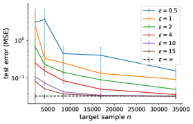
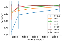
$\mathsf{CnvxAdap}$, (MSE): Gas	$\mathsf{NCnvxAdap}$, (Accuracy): Adult
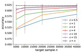
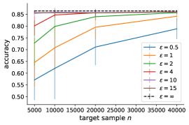
$\mathsf{NCnvxAdap}$, (Accuracy): CIFAR-100	$\mathsf{NCnvxAdap}$, (Accuracy): CIFAR-10

Figure 1: Performance of $\mathsf{CnvxAdap}$ and $\mathsf{NCnvxAdap}$ on various dataset against number of target samples for various values of $\epsilon$.

Figure 1(upper left panel) presents the MSE on the Gas dataset over ten runs against the number of target samples with various values of $\varepsilon$ as small as $0.5$. The dashed line corresponds to the non-private convex solution of $\mathsf{CnvxAdap}_{\infty}$. We observe that the performance of our private adaptation algorithm $\mathsf{CnvxAdap}$ approaches that of the non-private solution ($\varepsilon=\infty$), as $\varepsilon$ increases and as $n$ increases, thereby verifying our convergence and theoretical analyses. For $\varepsilon=10$ or $\varepsilon=15$, the performance of $\mathsf{CnvxAdap}$ is close to that of $\mathsf{CnvxAdap}_{\infty}$ for $n=10\mathord{,}000$. For reference, we also compared $\mathsf{CnvxAdap}$ with the noisy minibatch SGD from (Bassily et al., 2019), see Appendix E, Figure 2. We verify that our algorithm outperforms minibatch SGD, which only benefits from the target labeled data.

In Table 2 we report a series of results comparing our private adaptation algorithm $\mathsf{CnvxAdap}$ to the non-private baseline, the DM algorithm (Cortes and Mohri, 2014), on the multi-domain sentiment analysis dataset (Blitzer et al., 2007). For $\epsilon\!=\!4$ the performance of $\mathsf{CnvxAdap}$ is on par with the DM algorithm, and for as low a value as $\epsilon\!=\!10$, it clearly outperforms DM. See Appendix E for more details.

Table 2: MSE of $\mathsf{CnvxAdap}$ for $\epsilon\!=\!4$ and $\epsilon\!=\!10$ against the non-private DM algorithm on the sentiment analysis dataset.

Source	Target	$\mathsf{CnvxAdap}$	$\mathsf{CnvxAdap}$	DM
		($\varepsilon=4$)	($\varepsilon=10$)
	BOOKS	$1.649\pm 1.909$	$0.713\pm 0.625$	$0.778\pm 0.459$
KITCHEN	DVD	$0.832\pm 0.640$	$0.521\pm 0.354$	$1.396\pm 1.145$
	ELEC	$0.790\pm 0.153$	$0.555\pm 0.139$	$1.740\pm 1.483$
	DVD	$0.929\pm 0.365$	$0.637\pm 0.297$	$0.761\pm 0.562$
BOOKS	ELEC	$0.708\pm 0.092$	$0.485\pm 0.147$	$0.711\pm 0.320$
	KITCHEN	$0.796\pm 0.126$	$0.632\pm 0.181$	$0.956\pm 0.442$
	ELEC	$0.671\pm 0.120$	$0.429\pm 0.189$	$0.677\pm 0.231$
DVD	KITCHEN	$0.665\pm 0.197$	$0.453\pm 0.189$	$1.185\pm 0.753$
	BOOKS	$0.727\pm 0.288$	$0.430\pm 0.143$	$0.676\pm 0.812$
	KITCHEN	$0.671\pm 0.161$	$0.439\pm 0.141$	$1.389\pm 0.755$
ELEC	BOOKS	$0.743\pm 0.365$	$0.351\pm 0.204$	$0.884\pm 0.639$
	DVD	$0.755\pm 0.585$	$0.589\pm 0.495$	$0.843\pm 0.403$

Finally, despite the difference in scenario, as discussed in Section 1, in Appendix E we also compare our algorithm to the private DM (Bassily et al., 2022) and show that for low values of $\varepsilon$ and even high values of $n$, the private-DM does not outperform our algorithm.

Table 3: Accuracy of non-private non-convex algorithm against baselines. Best results are boldfaced.

Dataset	Train source	Train target	KMM	$\mathsf{NCnvxAdap}_{\infty}$
Adult	$88.44\pm 0.61$	$91.09\pm 0.54$	$74.62\pm 0.64$	$\mathbf{91.38\pm 0.49}$
German	$74.16\pm 1.64$	$76.40\pm 1.17$	$74.43\pm 1.65$	$\mathbf{77.96\pm 1.31}$
Accent	$51.60\pm 1.09$	$92.27\pm 1.10$	$52.18\pm 2.27$	$\mathbf{93.95\pm 0.78}$
CIFAR-100	$58.50\pm 0.30$	$59.51\pm 0.38$	$58.27\pm 0.28$	$\mathbf{62.19\pm 0.32}$
CIFAR-10	$83.18\pm 0.47$	$85.18\pm 0.24$	$83.57\pm 0.45$	$\mathbf{86.44\pm 0.29}$
SVHN	$84.16\pm 1.21$	$86.28\pm 0.44$	$84.13\pm 1.21$	$\mathbf{87.34\pm 0.46}$
ImageNet	$71.20\pm 1.75$	$85.70\pm 0.29$	$71.25\pm 1.77$	$\mathbf{86.84\pm 0.38}$

Non-private comparison to baselines. Classification. For the general non-convex setting, we experiment with logistic regression classifiers and consider seven datasets. Three datasets are from the UCI machine learning repository (Dua and Graff, 2017), the Adult, German and Accent (see Appendix E for the detailed information about these datasets). We also convert the CIFAR-100, CIFAR-10 (Krizhevsky, 2009), SVHN (Netzer et al., 2011) and ImageNet (Deng et al., 2009) datasets into domain adaptation tasks by establishing two distinct sampling methods for selecting the source and target data (see Appendix E.2 for more details). We first compare our non-private non-convex algorithm $\mathsf{NCnvxAdap}_{\infty}$ with the KMM algorithm (Huang et al., 2006). We report in Table 3 the mean and standard deviation of the accuracy on the test set over $10$ random splits of the target training (70%), validation (20%) and test sets (10%). The results show that our non-convex algorithm consistently outperforms the baseline.

Comparison of private and non-private algorithm. Classification. We then study the performance and convergence properties of $\mathsf{NCnvxAdap}$ as a function of the privacy guarantee $\epsilon$ and training sample size $n$. Figure 1 presents the accuracy on the Adult, the CIFAR-100, and the CIFAR-10 datasets over ten runs against the number of target samples with various values of $\varepsilon$. The dashed line corresponds to the non-private solution of $\mathsf{NCnvxAdap}_{\infty}$. We observe that the performance of our private algorithm approaches that of the non-private solution ($\varepsilon=\infty$), as $\varepsilon$ increases and as $n$ increases. For $\varepsilon=10$ or $\varepsilon=15$, the performance is close to the dashed line for $n=10\mathord{,}000$.

7 Conclusion

We presented two $(\varepsilon,\delta)$-differentially private algorithms for supervised adaptation based on strong theoretical learning guarantees. Our experimental results suggest that these algorithms can be effective in applications and scenarios where domain adaptation can be successful. Our proof and algorithmic techniques, such as our reparameterization, are likely to be useful in the analysis of other related problems (see Appendix F) including for the reverse problem of adaptation from a private source to a public target domain.

RB’s research is supported by NSF CAREER Award 2144532, NSF Award 2112471, and Google Faculty Research Award.

Appendix A Related work

There is a very broad literature on domain adaptation that we cannot survey in detail within this limited space. Thus, we refer the reader to surveys such as (Pan and Yang, 2009; Wang and Deng, 2018; Li, 2012) for a relatively comprehensive overview and briefly discuss approaches that are the most relevant to our study.

Our analysis admits a strong theoretical component since we seek a differentially private algorithm with theoretical learning and privacy guarantees. We benefit from several past publications already referenced that have given a theoretical analysis of adaptation using the notion of discrepancy. There are several other related publications using the notion of discrepancy for a PAC-Bayesian analysis (Germain et al., 2013) or active learning (de Mathelin et al., 2021). There are also other interesting theoretical analyses of adaptation such as (Hanneke and Kpotufe, 2019), which deals with the notions of super transfer or localization; these notions admit some connections with that of (local) discrepancy (Cortes et al., 2019; Zhang et al., 2020b).

In the privacy literature, several interesting algorithms have been given with formal differentially private learning guarantees, assuming access to public data (Chaudhuri and Hsu, 2011; Beimel et al., 2013; Bassily et al., 2018; Alon et al., 2019; Nandi and Bassily, 2020; Bassily et al., 2020). But these results cannot be used in the adaptation scenario we consider since they assume that the source and target domains coincide. A differentially private correlation alignment approach for domain adaptation was given by Jin et al. (2021) for a distinct scenario where both source and target data are private. More recently, Wang et al. (2020) described algorithms for deep domain adaptation for classification, but the authors do not provide theoretical guarantees for these algorithms.

The problem of private density estimation using a small amounto public data has been studied in several recent publications. Bie et al. (2022) studied the problem of estimating a $d$-dimensional Gaussian distribution, under the assumption of access to a Gaussian that may have vanishing similarity in total variation distance with the underlying Gaussian of the private data. Ben-David et al. (2023) studied the problem of private distribution learning with access to public data. They related private density estimation to sample compression schemes for distributions. They approximately recovered previous results on Gaussians, and presented other results such as sample complexity upper bounds for arbitrary $k$-mixtures of Gaussians. Tramèr et al. (2022) presented a general discussion of the question of private learning with large-scale public pretraining.

As discussed in the main text, the most closely related work to ours is the recent study of Bassily et al. (2022), which considers a similar adaptation scenario with a public source domain and a private target domain and which also gives private algorithms with theoretical guarantees. However, that work can be distinguished from ours in several aspects. First, the authors consider a purely unsupervised adaptation scenario where no labeled sample is available from the target domain, while we consider a supervised scenario. Our study and algorithms can be extended to the unsupervised or weakly supervised setting using the notion of unlabeled discrepancy (Mansour et al., 2009), by leveraging upper bounds on labeled discrepancy in terms of unlabeled discrepancy as in (Awasthi et al., 2024). Second, the learning guarantees of our private algorithms benefit from the recent optimization of Awasthi et al. (2024), which they show are theoretically stronger than those of the DM solution of Cortes and Mohri (2014) adopted by Bassily et al. (2022). Similarly, in our experiments, our convex optimization solution outperforms the DM algorithm. Note that the empirical study in (Bassily et al., 2022) is limited to a single specific artificial dataset, while we present empirical results with several non-artificial datasets. Third, our private adaptation algorithms include solutions both for regression and classification, while those of Bassily et al. (2022) are specifically given for regression with the squared loss.

Appendix B General analysis of supervised adaptation

In this section, we describe the general learning bound of Awasthi et al. (2024), for which we give a self-contained and concise proof. This bound holds for any sample reweighting method in domain adaptation. This includes as special cases a number of methods presented for adaptation in the past, including KMM (Huang et al., 2006), KLIEP (Sugiyama et al., 2007b), importance weighting with bounded weights (Cortes et al., 2010), discrepancy minimization (Cortes and Mohri, 2014), gapBoost algorithm (Wang et al., 2019), and many others. Next, we discuss the implications of this bound and the related optimization problem.

B.1 General learning bound

The learning bound draws on a natural extension of the notion of Rademacher complexity to the weighted case, ${\mathsf{q}}$-weighted Rademacher complexity, which is denoted by $\mathfrak{R}_{{\mathsf{q}}}(\ell\circ{\mathscr{H}})$ and defined by

$$\mathfrak{R}_{{\mathsf{q}}}(\ell\circ{\mathscr{H}})=\operatorname*{\mathbb{E}}_{S^{\mathsf{Pub}},S^{\mathsf{Priv}},{\boldsymbol{\sigma}}}\left[\sup_{h\in{\mathscr{H}}}\sum_{i=1}^{m+n}\sigma_{i}{\mathsf{q}}_{i}\ell(h(x_{i}),y_{i})\right],$$ (8)

where $\sigma_{i}$s are independent random variables uniformly distributed over $\{-1,+1\}$. The bound holds uniformly over both the choice of a hypothesis $h$ selected in ${\mathscr{H}}$ and that of a weight vector ${\mathsf{q}}$ in the open $\|\,\cdot\,\|_{1}$-ball of radius one centered in ${\mathsf{p}}^{0}$, ${\mathsf{B}}_{1}({\mathsf{p}}^{0},1)=\left\{{\mathsf{q}}\colon\|{\mathsf{q}}-{\mathsf{p}}^{0}\|_{1}<1\right\}$, where ${\mathsf{p}}^{0}$ can be interpreted as a reference or ideal reweighting choice.

Theorem B.1.

For any $\eta>0$, with probability at least $1-\eta$ over the draw of a sample $S^{\mathsf{Pub}}$ of size $m$ from ${\mathscr{D}}^{\mathsf{Pub}}$ and a sample $S^{\mathsf{Priv}}$ of size $n$ from ${\mathscr{D}}^{\mathsf{Priv}}$, the following holds for all $h\in{\mathscr{H}}$ and ${\mathsf{q}}\in{\mathsf{B}}_{1}({\mathsf{p}}^{0},1)$:

$$\mathcal{L}({\mathscr{D}}^{\mathsf{Priv}},h) \leq\sum_{i=1}^{m+n}{\mathsf{q}}_{i}\ell(h(x_{i}),y_{i})+\overline{\mathsf{q}}^{\mathsf{Pub}}\mathrm{dis}\left({\mathscr{D}}^{\mathsf{Priv}},{\mathscr{D}}^{\mathsf{Pub}}\right)+2\mathfrak{R}_{{\mathsf{q}}}(\ell\circ{\mathscr{H}})+6B\|{\mathsf{q}}-{\mathsf{p}}^{0}\|_{1}$$

$$\quad+B\left[\|{\mathsf{q}}\|_{2}+2\|{\mathsf{q}}-{\mathsf{p}}^{0}\|_{1}\right]\left[\sqrt{\log\log_{2}\tfrac{2}{1-\|{\mathsf{q}}-{\mathsf{p}}^{0}\|_{1}}}+\sqrt{\tfrac{\log(2/\eta)}{2}}\right].$$

Proof B.2.

The proof of theorem consists of first deriving a ${\mathsf{q}}$-weighted Rademacher complexity bound for a fixed reweighting ${\mathsf{q}}$, using the fact that the expectation of the empirical term is then

$$\left(\overline{\mathsf{q}}^{\mathsf{Pub}}\mathcal{L}({\mathscr{D}}^{\mathsf{Pub}},h)+\overline{\mathsf{q}}^{\mathsf{Priv}}\mathcal{L}({\mathscr{D}}^{\mathsf{Priv}},h)\right).$$

Next, the difference of ${\mathsf{q}}^{\mathsf{Priv}}\mathcal{L}({\mathscr{D}}^{\mathsf{Priv}},h)$ and this term is analyzed in terms of the discrepancy term $\overline{\mathsf{q}}^{\mathsf{Pub}}\mathrm{dis}\left({\mathscr{D}}^{\mathsf{Priv}},{\mathscr{D}}^{\mathsf{Pub}}\right)$ and then the bound is extended to hold uniformly over ${\mathsf{B}}_{1}({\mathsf{p}}^{0},1)$, using a technique similar to that of deriving uniform margin bounds, see for example (Mohri et al., 2018)[Chapter 5]. We will use $S$ to refer to the full sample: $S=(S^{\mathsf{Pub}},S^{\mathsf{Priv}})$ and will use the shorthand $\mathcal{L}_{S}({\mathsf{q}},h)=\sum_{i=1}^{m+n}{\mathsf{q}}_{i}\ell(h(x_{i}),y_{i})$ for the empirical term.

Fix ${\mathsf{q}}\in[0,1]^{m+n}$. The expectation of $\mathcal{L}_{S}({\mathsf{q}},h)$ over the draw of $(S^{\mathsf{Pub}},S^{\mathsf{Priv}})\sim({\mathscr{D}}^{\mathsf{Pub}})^{m}\times({\mathscr{D}}^{\mathsf{Pub}})^{n}$ is then given by

$$\operatorname*{\mathbb{E}}_{S}[\mathcal{L}_{S}({\mathsf{q}},h)] =\sum_{i=1}^{m}{\mathsf{q}}_{i}\operatorname*{\mathbb{E}}_{S^{\mathsf{Pub}}}[\ell(h(x_{i}),y_{i})]+\sum_{i=m+1}^{m+n}{\mathsf{q}}_{i}\operatorname*{\mathbb{E}}_{S^{\mathsf{Priv}}}[\ell(h(x_{i}),y_{i})]$$

$$=\sum_{i=1}^{m}{\mathsf{q}}_{i}\mathcal{L}({\mathscr{D}}^{\mathsf{Pub}},h)+\sum_{i=m+1}^{m+n}{\mathsf{q}}_{i}\mathcal{L}({\mathscr{D}}^{\mathsf{Priv}},h)$$

$$=\overline{\mathsf{q}}^{\mathsf{Pub}}\mathcal{L}({\mathscr{D}}^{\mathsf{Pub}},h)+\overline{\mathsf{q}}^{\mathsf{Priv}}\mathcal{L}({\mathscr{D}}^{\mathsf{Priv}},h).$$

Consider $\Psi(S)=\sup_{h\in{\mathscr{H}}}\left\{\overline{\mathsf{q}}^{\mathsf{Pub}}\mathcal{L}({\mathscr{D}}^{\mathsf{Pub}},h)+\overline{\mathsf{q}}^{\mathsf{Priv}}\mathcal{L}({\mathscr{D}}^{\mathsf{Priv}},h)-\mathcal{L}_{S}({\mathsf{q}},h)\right\}$. Changing point $x_{i}$ to $x^{\prime}_{i}$ affects $\Psi(S)$ at most by ${\mathsf{q}}_{i}B$, since the loss is bounded by $B$. It is also not hard to see that the standard symmetrization argument (see (Mohri et al., 2018)) can be extended to the weighted case and that $\operatorname*{\mathbb{E}}_{S}[\Psi(S)]\leq 2\mathfrak{R}_{\mathsf{q}}(\ell\circ{\mathscr{H}})$. Thus, by McDiarmid’s inequality, for any $\eta>0$, with probability at least $1-\eta$, the following holds:

$$\overline{\mathsf{q}}^{\mathsf{Pub}}\mathcal{L}({\mathscr{D}}^{\mathsf{Pub}},h)+\overline{\mathsf{q}}^{\mathsf{Priv}}\mathcal{L}({\mathscr{D}}^{\mathsf{Priv}},h)-\mathcal{L}_{S}({\mathsf{q}},h)\leq 2\mathfrak{R}_{\mathsf{q}}(\ell\circ{\mathscr{H}})+B\sqrt{\frac{\log\frac{1}{\eta}}{2m}}.$$ (9)

Now, we can also analyze the difference of $\mathcal{L}({\mathscr{D}}^{\mathsf{Priv}},h)$ and $\overline{\mathsf{q}}^{\mathsf{Pub}}\mathcal{L}({\mathscr{D}}^{\mathsf{Pub}},h)+\overline{\mathsf{q}}^{\mathsf{Priv}}\mathcal{L}({\mathscr{D}}^{\mathsf{Priv}},h)$ as follows:

$$\mathcal{L}({\mathscr{D}}^{\mathsf{Priv}},h)-\left(\overline{\mathsf{q}}^{\mathsf{Pub}}\mathcal{L}({\mathscr{D}}^{\mathsf{Pub}},h)+\overline{\mathsf{q}}^{\mathsf{Priv}}\mathcal{L}({\mathscr{D}}^{\mathsf{Priv}},h)\right)$$

$$=(1-\overline{\mathsf{q}}^{\mathsf{Priv}})\mathcal{L}({\mathscr{D}}^{\mathsf{Priv}},h)-\overline{\mathsf{q}}^{\mathsf{Pub}}\mathcal{L}({\mathscr{D}}^{\mathsf{Pub}},h)$$

$$=(1-\overline{\mathsf{q}}^{\mathsf{Priv}}-\overline{\mathsf{q}}^{\mathsf{Pub}})\mathcal{L}({\mathscr{D}}^{\mathsf{Priv}},h)+\overline{\mathsf{q}}^{\mathsf{Pub}}(\mathcal{L}({\mathscr{D}}^{\mathsf{Priv}},h)-\mathcal{L}({\mathscr{D}}^{\mathsf{Pub}},h))$$

$$=(\|{\mathsf{p}}^{0}\|_{1}-\|{\mathsf{q}}\|_{1})\mathcal{L}({\mathscr{D}}^{\mathsf{Priv}},h)+\overline{\mathsf{q}}^{\mathsf{Pub}}(\mathcal{L}({\mathscr{D}}^{\mathsf{Priv}},h)-\mathcal{L}({\mathscr{D}}^{\mathsf{Pub}},h))$$

$$\leq B\|{\mathsf{p}}^{0}-{\mathsf{q}}\|_{1}+\overline{\mathsf{q}}^{\mathsf{Pub}}\mathrm{dis}({\mathscr{D}}^{\mathsf{Priv}},{\mathscr{D}}^{\mathsf{Pub}}).$$ (10)

Combining (9) and (10) yields the following high-probability inequality for a fixed ${\mathsf{q}}$:

$$\mathcal{L}({\mathscr{D}}^{\mathsf{Priv}},h)\leq\mathcal{L}_{S}({\mathsf{q}},h)+2B\|{\mathsf{p}}^{0}-{\mathsf{q}}\|_{1}+\overline{\mathsf{q}}^{\mathsf{Pub}}\mathrm{dis}({\mathscr{D}}^{\mathsf{Priv}},{\mathscr{D}}^{\mathsf{Pub}})+\mathfrak{R}_{\mathsf{q}}(\ell\circ{\mathscr{H}})+B\sqrt{\frac{\log\frac{1}{\eta}}{2m}}.$$ (11)

Consider a sequence of weight vectors ${\mathsf{q}}_{k}\in[0,1]^{m+n}$ and a sequence of confidence weights $\eta_{k}=\frac{\eta}{2^{k+1}}$. Inequality (11), with ${\mathsf{q}}$ replaced by ${\mathsf{q}}^{k}$ and $\eta$ replaced by $\eta_{k}$, holds for each $k\geq 0$, with probability $1-\eta_{k}$. Thus, by the union bound, since $\sum_{k=0}^{+\infty}\frac{\eta}{2^{k+1}}=\eta$, with probability $1-\eta$, it holds for all $k\geq 0$.

$$\mathcal{L}({\mathscr{D}}^{\mathsf{Priv}},h)\leq\mathcal{L}_{S}({\mathsf{q}}^{k},h)+2B\|{\mathsf{p}}^{0}-{\mathsf{q}}^{k}\|_{1}+\overline{\mathsf{q}}^{k,\mathsf{Pub}}\mathrm{dis}({\mathscr{D}}^{\mathsf{Priv}},{\mathscr{D}}^{\mathsf{Pub}})+\mathfrak{R}_{{\mathsf{q}}^{k}}(\ell\circ{\mathscr{H}})+B\sqrt{\frac{\log\frac{1}{\eta}}{2m}}.$$ (12)

We can choose ${\mathsf{q}}^{k}$ such that $\|{\mathsf{q}}^{k}-{\mathsf{p}}^{0}\|_{1}=1-\frac{1}{2^{k}}$. Then, for any ${\mathsf{q}}\in{\mathsf{B}}({\mathsf{p}}^{0},1)$, there exists $k\geq 0$ such that $\|{\mathsf{q}}^{k}-{\mathsf{p}}^{0}\|_{1}\leq\|{\mathsf{q}}-{\mathsf{p}}^{0}\|_{1}<\|{\mathsf{q}}^{k+1}-{\mathsf{p}}^{0}\|_{1}$ and thus such that

$$\sqrt{2\log(k+1)}=\sqrt{2\log\log_{2}\frac{2}{1-\|{\mathsf{q}}^{k}-{\mathsf{p}}^{0}\|_{1}}} \leq\sqrt{2\log\log_{2}\frac{2}{1-\|{\mathsf{q}}-{\mathsf{p}}^{0}\|_{1}}}.$$

Furthermore, for that $k$, the following inequalities hold:

$$\mathcal{L}_{S}({\mathsf{q}}^{k},h) \leq\sum_{i=1}^{m+n}{\mathsf{q}}_{i}\ell(h(x_{i}),y_{i})+B\|{\mathsf{q}}^{k}-{\mathsf{q}}\|_{1}\leq\mathcal{L}_{S}({\mathsf{q}},h)+2B\|{\mathsf{p}}^{0}-{\mathsf{q}}\|_{1}$$

$$\overline{\mathsf{q}}^{k,\mathsf{Pub}} \leq\overline{\mathsf{q}}^{\mathsf{Pub}}+\|{\mathsf{q}}^{k}-{\mathsf{q}}\|_{1}\leq\overline{\mathsf{q}}^{\mathsf{Pub}}+2\|{\mathsf{p}}^{0}-{\mathsf{q}}\|_{1}$$

$$\mathfrak{R}_{{\mathsf{q}}^{k}}(\ell\circ{\mathscr{H}}) \leq\mathfrak{R}_{{\mathsf{q}}}(\ell\circ{\mathscr{H}})+B\|{\mathsf{q}}^{k}-{\mathsf{q}}\|_{1}\leq\mathfrak{R}_{{\mathsf{q}}}(\ell\circ{\mathscr{H}})+2B\|{\mathsf{q}}-{\mathsf{p}}^{0}\|_{1},$$

$$\|{\mathsf{q}}^{k}\|_{2} \leq\|{\mathsf{q}}\|_{2}+\|{\mathsf{q}}^{k}-{\mathsf{q}}\|_{2}\leq\|{\mathsf{q}}\|_{2}+\|{\mathsf{q}}^{k}-{\mathsf{q}}\|_{1}\leq\|{\mathsf{q}}\|_{2}+2\|{\mathsf{q}}-{\mathsf{p}}^{0}\|_{1}.$$

Plugging in these inequalities in (12) completes the proof.

B.2 Optimization problem

The bound suggests the following to achieve a good generalization error in adaptation: ensure a small ${\mathsf{q}}$-empirical loss (first term), but not at the price of a too sparse weight vector, which would result in a larger $\|{\mathsf{q}}\|_{2}$ (fifth term); allocate a smaller total weight to public points when the discrepancy is larger (second term); limit the ${\mathsf{q}}$-weighted complexity of the hypothesis set ${\mathscr{H}}$ combined with the loss function $\ell$ (third term); and ensure the closeness of ${\mathsf{q}}$ to the reference weight vector ${\mathsf{p}}^{0}$ (fourth and fifth terms).

The joint optimization problem (3) is directly based on minimizing the right-hand side of the inequality over the choice of both $h\in{\mathscr{H}}$ and ${\mathsf{q}}\in{\mathsf{B}}_{1}({\mathsf{p}}^{0},1)$. By McDiarmid’s inequality, the discrepancy term $\mathrm{dis}\left({\mathscr{D}}^{\mathsf{Priv}},{\mathscr{D}}^{\mathsf{Pub}}\right)$ can be replaced by its estimate $\hat{d}$ (2) from finite sample modulo a term in $O(\sqrt{\frac{m+n}{mn}})$. Instead of the supremum over the full family ${\mathscr{H}}$, one can also use a local discrepancy Cortes et al. (2019); de Mathelin et al. (2021); Zhang et al. (2019, 2020b) and restrict oneself to a ball around the empirical minimizer of the private loss of radius $O(1/\sqrt{n})$. Using Talagrand’s inequality (Ledoux and Talagrand, 1991) and the straightforward observation that for any $i$, $x\mapsto{\mathsf{q}}_{i}x$ is $\|{\mathsf{q}}\|_{\infty}$-Lipschitz, the weighted Rademacher complexity bound can be upper bounded by $\|{\mathsf{q}}\|_{\infty}(m+n)\mathfrak{R}_{m+n}(\ell\circ{\mathscr{H}})$, where $\mathfrak{R}_{m+n}(\ell\circ{\mathscr{H}})$ is the standard (unweighted) Rademacher complexity of the family of loss functions over the hypothesis set ${\mathscr{H}}$. For uniform weights, this is an equality. Thus, using the upper bounds just discussed and replacing constants with hyperparameters, minimizing the right-hand side of the learning bounds of Theorem B.1 can be formulated as the joint optimization problem (3).

Appendix C Proofs of Section 4

C.1 Proof of Lemma 4.1

See 4.1

Proof C.1.

First observe that the following inequalities hold:

$$\|\nabla_{w}{\mathsf{F}}(w,{\mathsf{u}})\|_{2} \leq\sum_{i=1}^{m+n}\frac{\|\nabla_{w}\ell_{\mathsf{sq}}(w,(x_{i},y_{i}))\|_{2}}{{\mathsf{u}}_{i}}\leq G\sum_{i=1}^{n+m}\frac{1}{{\mathsf{u}}_{i}}\leq G,$$

where the second inequality follows from the $G$-Lipschitzness of the loss, and the third from the constraints on ${\mathsf{u}}$: $\frac{1}{{\mathsf{u}}_{i}}\leq\frac{\alpha}{m},\forall i\in[m]$ and $\frac{1}{{\mathsf{u}}_{i}}\leq\frac{1-\alpha}{n},\forall i\in[m+1,m+n]$.

Next, note that we have

$$\left\lvert\frac{\partial{\mathsf{F}}(w,{\mathsf{u}})}{\partial{\mathsf{u}}^{\mathsf{Pub}}_{i}}\right\rvert \leq\frac{2B}{\left({\mathsf{u}}^{\mathsf{Pub}}_{i}\right)^{2}}+\kappa_{1}\frac{\alpha^{2}}{m}+\kappa_{2}\frac{\frac{1}{\left({\mathsf{u}}^{\mathsf{Pub}}_{i}\right)^{3}}}{\sqrt{\sum_{i=1}^{m+n}\frac{1}{\left({\mathsf{u}}^{\mathsf{Pub}}_{i}\right)^{2}}}}+\kappa_{\infty}\frac{1\left(i\in\operatorname*{argmin}_{j\in[m+n]}{\mathsf{u}}_{j}\right)}{\left({\mathsf{u}}^{\mathsf{Pub}}_{i}\right)^{2}}$$

$$\leq\frac{2B}{\left({\mathsf{u}}^{\mathsf{Pub}}_{i}\right)^{2}}+\kappa_{1}\frac{\alpha^{2}}{m}+\frac{\kappa_{2}}{\left({\mathsf{u}}^{\mathsf{Pub}}_{i}\right)^{2}}+\frac{\kappa_{\infty}}{\left({\mathsf{u}}^{\mathsf{Pub}}_{i}\right)^{2}}$$

$$\leq\frac{\alpha^{2}}{m^{2}}\left(2B+\kappa_{1}+\kappa_{2}+\kappa_{\infty}\right),$$

where the first inequality follows from the fact that the loss is uniformly bounded by $B$, and hence $\ell_{\mathsf{sq}}(w,(x_{i},y_{i}))+\hat{d}_{\textsc{DP}}\,1_{i\leq m}\leq 2B$. The remaining steps follow straightforwardly from the constraints on ${\mathsf{u}}^{\mathsf{Pub}}$. Thus, we have $\|\nabla_{{\mathsf{u}}^{\mathsf{Pub}}}{\mathsf{F}}(w,{\mathsf{u}}^{\mathsf{Pub}})\|_{2}\leq\frac{\alpha^{2}}{m^{3/2}}\left(2B+\kappa_{1}+\kappa_{2}+\kappa_{\infty}\right)$.

Similarly, we have $\left\lvert\frac{\partial{\mathsf{F}}(w,{\mathsf{u}})}{\partial{\mathsf{u}}^{\mathsf{Priv}}_{i}}\right\rvert\leq\frac{(1-\alpha)^{2}}{n^{2}}\left(B+\kappa_{1}+\kappa_{2}+\kappa_{\infty}\right)$ and thus

$$\|\nabla_{{\mathsf{u}}^{\mathsf{Priv}}}{\mathsf{F}}(w,{\mathsf{u}}^{\mathsf{Priv}})\|_{2}\leq\frac{(1-\alpha)^{2}}{n^{3/2}}\left(B+\kappa_{1}+\kappa_{2}+\kappa_{\infty}\right).$$

This proves the first item of the lemma.

Second, we bound the $\ell_{2}$-sensitivity of $\nabla_{w}\widehat{L}^{\mathsf{Priv}}(w,{\mathsf{u}}^{\mathsf{Priv}})$ and $\nabla_{{\mathsf{u}}^{\mathsf{Priv}}}\widehat{L}^{\mathsf{Priv}}(w,{\mathsf{u}}^{\mathsf{Priv}})$. Consider any pair of neighboring private datasets $S^{\mathsf{Priv}}$ and $\bar{S}^{\mathsf{Priv}}$. Let $(x^{\mathsf{Priv}}_{j},y^{\mathsf{Priv}}_{j})$ and $(\bar{x}^{\mathsf{Priv}}_{j},\bar{y}^{\mathsf{Priv}}_{j})$ be the data points by which the two datasets differ. To emphasize the dependence on the dataset, we will denote $\nabla_{w}\widehat{L}^{\mathsf{Priv}}(w,{\mathsf{u}}^{\mathsf{Priv}})$ with respect to dataset $S$ as $\nabla_{w}\widehat{L}^{\mathsf{Priv}}(w,{\mathsf{u}}^{\mathsf{Priv}};S)$. We can write:

$$\mspace{-80.0mu}\left\|\nabla_{w}\widehat{L}^{\mathsf{Priv}}(w,{\mathsf{u}}^{\mathsf{Priv}};S^{\mathsf{Priv}})-\nabla_{w}\widehat{L}^{\mathsf{Priv}}(w,{\mathsf{u}}^{\mathsf{Priv}};\bar{S}^{\mathsf{Priv}})\right\|_{2}$$

$$=\frac{\left\|\nabla_{w}\ell_{\mathsf{sq}}(w,(x^{\mathsf{Priv}}_{j},y^{\mathsf{Priv}}_{j}))-\nabla_{w}\ell_{\mathsf{sq}}(w,(\bar{x}^{\mathsf{Priv}}_{j},\bar{y}^{\mathsf{Priv}}_{j}))\right\|_{2}}{{\mathsf{u}}^{\mathsf{Priv}}_{j}}$$

$$\leq\frac{2G(1-\alpha)}{n}.$$

Similarly, we can write:

$$\mspace{-80.0mu}\left\|\nabla_{{\mathsf{u}}^{\mathsf{Priv}}}\widehat{L}^{\mathsf{Priv}}(w,{\mathsf{u}}^{\mathsf{Priv}};S^{\mathsf{Priv}})-\nabla_{{\mathsf{u}}^{\mathsf{Priv}}}\widehat{L}^{\mathsf{Priv}}(w,{\mathsf{u}}^{\mathsf{Priv}};\bar{S}^{\mathsf{Priv}})\right\|_{2}$$

$$=\left\lvert\frac{\ell_{\mathsf{sq}}(w,(x^{\mathsf{Priv}}_{j},y^{\mathsf{Priv}}_{j}))-\ell_{\mathsf{sq}}(w,(\bar{x}^{\mathsf{Priv}}_{j},\bar{y}^{\mathsf{Priv}}_{j}))}{\left({\mathsf{u}}^{\mathsf{Priv}}_{j}\right)^{2}}\right\rvert$$

$$\leq\frac{B(1-\alpha)^{2}}{n^{2}}.$$

This completes the proof.

C.2 Proof of Theorem 4.2

See 4.2

We will show more precisely the following inequality:

$$\mspace{-40.0mu}\underset{}{\mathbb{E}}\left[{\mathsf{F}}(\bar{w},\bar{{\mathsf{u}}})-{\mathsf{F}}(w^{\ast},{\mathsf{u}}^{\ast})\right]$$

$$\leq\Lambda G\sqrt{\frac{1}{T}+\frac{32(1-\alpha)^{2}d\log(\frac{2}{\delta})}{n^{2}\varepsilon^{2}}}$$

$$\quad+\frac{(1-\alpha)^{2}\left(U^{\mathsf{Priv}}+1\right)}{2n^{3/2}}\sqrt{\frac{\bar{B}^{2}}{T}+\frac{8B^{2}\log(\frac{2}{\delta})}{\varepsilon^{2}}}$$

$$\quad+\frac{\alpha^{2}\left(U^{\mathsf{Pub}}+1\right)(B+\bar{B})}{2m^{3/2}\sqrt{T}},$$

where ${\mathsf{u}}^{\ast}=\left({\mathsf{u}}^{\mathsf{Pub}\ast},{\mathsf{u}}^{\mathsf{Priv}\ast}\right)$, $U^{\mathsf{Priv}}\triangleq\|{\mathsf{u}}^{\mathsf{Priv}}_{0}-{\mathsf{u}}^{\mathsf{Priv}\ast}\|_{2}^{2}$, and $U^{\mathsf{Pub}}\triangleq\|{\mathsf{u}}^{\mathsf{Pub}}_{0}-{\mathsf{u}}^{\mathsf{Pub}\ast}\|_{2}^{2}$.

Proof C.2.

First, we show the privacy guarantee. Note that for any iteration $t\in[T]$, the only quantities that depend on the private dataset are the gradient components $\nabla_{w}{\mathsf{F}}(w_{t},{\mathsf{u}}_{t})$ and $\nabla_{{\mathsf{u}}^{\mathsf{Priv}}}{\mathsf{F}}(w_{t},{\mathsf{u}}_{t})$. From the guarantees on the $\ell_{2}$-sensitivity of these gradient components given by parts 2 and 3 of Lemma 4.1 and by the properties of the Gaussian mechanism of differential privacy, each iteration $t\in[T]$ of Algorithm 1 is $(\frac{\varepsilon}{\sqrt{T}},\delta)$-differentially private. Now, using the moments accountant technique of Abadi et al. (2016) to account for the composition over the $T$ iterations of the algorithm, which applies to Gaussian noise, Algorithm 1 is $(\varepsilon,\delta)$-differentially private. Note that we could have also resorted to the advanced composition theorem of differential privacy, but the moments accountant technique leads to a tighter privacy analysis; in particular, it allows us to save a $\sqrt{\log(1/\delta)}$-factor in the final $\varepsilon$ and $T$ factor in the final $\delta$ privacy parameters.

Next, we prove the bound on the optimization error. The proof involves some tweaks of the the standard analysis of the (stochastic) projected gradient descent algorithm for convex objectives. In particular, our proof entails decomposing each gradient $\nabla{\mathsf{F}}$ into its three components $\nabla_{w}{\mathsf{F}},\nabla_{{\mathsf{u}}^{\mathsf{Pub}}}{\mathsf{F}},$ and $\nabla{\mathsf{F}}_{{\mathsf{u}}^{\mathsf{Priv}}}$ to allow for introducing a different step size for updating each of $w,{\mathsf{u}}^{\mathsf{Pub}}$ and ${\mathsf{u}}^{\mathsf{Priv}}$. By a standard argument, we have

$$\mspace{-20.0mu}\underset{}{\mathbb{E}}\left[\|w_{t+1}-w^{\ast}\|_{2}^{2}\right]$$

$$\leq\underset{}{\mathbb{E}}\left[\|w_{t}-w^{\ast}\|_{2}^{2}\right]-2\eta_{w}\underset{}{\mathbb{E}}\left[\langle\nabla_{w}{\mathsf{F}}(w_{t},{\mathsf{u}}_{t})+{\mathbf{z}}_{t},w_{t}-w^{\ast}\rangle\right]+\eta_{w}^{2}\underset{}{\mathbb{E}}\left[\|\nabla_{w}{\mathsf{F}}(w_{t},{\mathsf{u}}_{t})+{\mathbf{z}}_{t}\|_{2}^{2}\right]$$

$$=\underset{}{\mathbb{E}}\left[\|w_{t}-w^{\ast}\|_{2}^{2}\right]-2\eta_{w}\underset{}{\mathbb{E}}\left[\langle\nabla_{w}{\mathsf{F}}(w_{t},{\mathsf{u}}_{t}),w_{t}-w^{\ast}\rangle\right]+\eta_{w}^{2}\underset{}{\mathbb{E}}\left[\|\nabla_{w}{\mathsf{F}}(w_{t},{\mathsf{u}}_{t})+{\mathbf{z}}_{t}\|_{2}^{2}\right]$$

$$\leq\underset{}{\mathbb{E}}\left[\|w_{t}-w^{\ast}\|_{2}^{2}\right]-2\eta_{w}\underset{}{\mathbb{E}}\left[\langle\nabla_{w}{\mathsf{F}}(w_{t},{\mathsf{u}}_{t}),w_{t}-w^{\ast}\rangle\right]+\eta_{w}^{2}\left(G^{2}+\sigma_{1}^{2}d\right),$$

where the second step follows from the linearity of expectation and the fact that ${\mathbf{z}}_{t}$ is independent of $\left((w_{0},{\mathsf{u}}_{0}),\ldots,(w_{t},{\mathsf{u}}_{t})\right)$ and that ${\mathbf{z}}_{t}$ has zero mean, and the last step follows from the fact that $\|\nabla_{w}{\mathsf{F}}(w_{t},{\mathsf{u}}_{t})\|^{2}_{2}\leq G^{2}$ proved in Lemma 4.1 and the fact that $\|{\mathbf{z}}_{t}\|_{2}^{2}=\sigma_{1}^{2}d.$ Hence,

$$\underset{}{\mathbb{E}}\left[\langle\nabla_{w}{\mathsf{F}}(w_{t},{\mathsf{u}}_{t}),w_{t}-w^{\ast}\rangle\right] \leq\frac{\underset{}{\mathbb{E}}\left[\|w_{t}-w^{\ast}\|_{2}^{2}\right]-\underset{}{\mathbb{E}}\left[\|w_{t+1}-w^{\ast}\|_{2}^{2}\right]}{2\eta_{w}}+\frac{\eta_{w}}{2}\left(G^{2}+\sigma_{1}^{2}d\right)$$ (13)

By a similar argument for $\|{\mathsf{u}}^{\mathsf{Pub}}_{t+1}-{\mathsf{u}}^{\mathsf{Pub}}_{t}\|^{2}_{2}$ and $\|{\mathsf{u}}^{\mathsf{Priv}}_{t+1}-{\mathsf{u}}^{\mathsf{Priv}}_{t}\|^{2}_{2}$ and using Lemma 4.1, we get

$$\mspace{-20.0mu}\underset{}{\mathbb{E}}\left[\langle\nabla_{{\mathsf{u}}^{\mathsf{Pub}}}{\mathsf{F}}(w_{t},{\mathsf{u}}_{t}),{\mathsf{u}}^{\mathsf{Pub}}_{t}-{\mathsf{u}}^{\mathsf{Pub}\ast}\rangle\right]$$

$$\leq\frac{\underset{}{\mathbb{E}}\left[\|{\mathsf{u}}^{\mathsf{Pub}}_{t}-{\mathsf{u}}^{\mathsf{Pub}\ast}\|_{2}^{2}\right]-\underset{}{\mathbb{E}}\left[\|{\mathsf{u}}^{\mathsf{Pub}}_{t+1}-{\mathsf{u}}^{\mathsf{Pub}\ast}\|_{2}^{2}\right]}{2\eta_{{\mathsf{u}}^{\mathsf{Pub}}}}+\frac{\eta_{{\mathsf{u}}^{\mathsf{Pub}}}}{2}\underset{}{\mathbb{E}}\left[\|\nabla_{{\mathsf{u}}^{\mathsf{Pub}}}{\mathsf{F}}(w_{t},{\mathsf{u}}_{t})\|_{2}^{2}\right]$$

$$\leq\frac{\underset{}{\mathbb{E}}\left[\|{\mathsf{u}}^{\mathsf{Pub}}_{t}-{\mathsf{u}}^{\mathsf{Pub}\ast}\|_{2}^{2}\right]-\underset{}{\mathbb{E}}\left[\|{\mathsf{u}}^{\mathsf{Pub}}_{t+1}-{\mathsf{u}}^{\mathsf{Pub}\ast}\|_{2}^{2}\right]}{2\eta_{{\mathsf{u}}^{\mathsf{Pub}}}}+\frac{\eta_{{\mathsf{u}}^{\mathsf{Pub}}}}{2}\cdot\frac{\alpha^{4}(\bar{B}+B)^{2}}{m^{3}}$$ (14)

$$\mspace{-20.0mu}\underset{}{\mathbb{E}}\left[\langle\nabla_{{\mathsf{u}}^{\mathsf{Priv}}}{\mathsf{F}}(w_{t},{\mathsf{u}}_{t}),{\mathsf{u}}^{\mathsf{Priv}}_{t}-{\mathsf{u}}^{\mathsf{Priv}\ast}\rangle\right]$$

$$\leq\frac{\underset{}{\mathbb{E}}\left[\|{\mathsf{u}}^{\mathsf{Priv}}_{t}-{\mathsf{u}}^{\mathsf{Priv}\ast}\|_{2}^{2}\right]-\underset{}{\mathbb{E}}\left[\|{\mathsf{u}}^{\mathsf{Priv}}_{t+1}-{\mathsf{u}}^{\mathsf{Priv}\ast}\|_{2}^{2}\right]}{2\eta_{{\mathsf{u}}^{\mathsf{Priv}}}}+\frac{\eta_{{\mathsf{u}}^{\mathsf{Priv}}}}{2}\underset{}{\mathbb{E}}\left[\|\nabla_{{\mathsf{u}}^{\mathsf{Priv}}}{\mathsf{F}}(w_{t},{\mathsf{u}}_{t})+{\mathbf{z}}_{t}^{\prime}\|_{2}^{2}\right]$$

$$\leq\frac{\underset{}{\mathbb{E}}\left[\|{\mathsf{u}}^{\mathsf{Priv}}_{t}-{\mathsf{u}}^{\mathsf{Priv}\ast}\|_{2}^{2}\right]-\underset{}{\mathbb{E}}\left[\|{\mathsf{u}}^{\mathsf{Priv}}_{t+1}-{\mathsf{u}}^{\mathsf{Priv}\ast}\|_{2}^{2}\right]}{2\eta_{{\mathsf{u}}^{\mathsf{Priv}}}}+\frac{\eta_{{\mathsf{u}}^{\mathsf{Priv}}}}{2}\left(\frac{(1-\alpha)^{4}\bar{B}^{2}}{n^{3}}+\sigma_{2}^{2}n\right)$$ (15)

By convexity of ${\mathsf{F}}$, we have

$$\underset{}{\mathbb{E}}\left[{\mathsf{F}}(w_{t},{\mathsf{u}}_{t})-{\mathsf{F}}(w^{\ast},{\mathsf{u}}^{\ast})\right] \leq\underset{}{\mathbb{E}}\left[\langle\nabla{\mathsf{F}}(w_{t},{\mathsf{u}}_{t}),~{}(w_{t},{\mathsf{u}}_{t})-(w^{\ast},{\mathsf{u}}^{\ast})\rangle\right]$$ (16)

$$=\underset{}{\mathbb{E}}\left[\langle\nabla_{w}{\mathsf{F}}(w_{t},{\mathsf{u}}_{t}),w_{t}-w^{\ast}\rangle\right]+\underset{}{\mathbb{E}}\left[\langle\nabla_{{\mathsf{u}}^{\mathsf{Pub}}}{\mathsf{F}}(w_{t},{\mathsf{u}}_{t}),{\mathsf{u}}^{\mathsf{Pub}}_{t}-{\mathsf{u}}^{\mathsf{Pub}\ast}\rangle\right]$$ (17)

$$~{}~{}+\underset{}{\mathbb{E}}\left[\langle\nabla_{{\mathsf{u}}^{\mathsf{Priv}}}{\mathsf{F}}(w_{t},{\mathsf{u}}_{t}),{\mathsf{u}}^{\mathsf{Priv}}_{t}-{\mathsf{u}}^{\mathsf{Priv}\ast}\rangle\right]$$ (18)

As in the standard analysis of gradient descent for convex objectives, we combine (18) with (13), (14), and (15), and use the fact that ${\mathsf{F}}(\bar{w},\bar{{\mathsf{u}}})-{\mathsf{F}}(w^{\ast},{\mathsf{u}}^{\ast})\leq\frac{1}{T}\sum_{t=1}^{T}\left({\mathsf{F}}(w_{t},{\mathsf{u}}_{t})-{\mathsf{F}}(w^{\ast},{\mathsf{u}}^{\ast})\right)$ (which follows from the convexity of ${\mathsf{F}}$) to arrive at

$$\underset{}{\mathbb{E}}\left[{\mathsf{F}}(\bar{w},\bar{{\mathsf{u}}})-{\mathsf{F}}(w^{\ast},{\mathsf{u}}^{\ast})\right]\leq \frac{\Lambda^{2}}{2\eta_{w}T}+\frac{\eta_{w}}{2}(G^{2}+d\sigma_{1}^{2})+\frac{U^{\mathsf{Priv}}}{2\eta_{{\mathsf{u}}^{\mathsf{Priv}}}T}+\frac{\eta_{{\mathsf{u}}^{\mathsf{Priv}}}}{2}\left(\frac{(1-\alpha)^{4}\bar{B}^{2}}{n^{3}}+n\sigma_{2}^{2}\right)$$

$$+\frac{U^{\mathsf{Pub}}}{2\eta_{{\mathsf{u}}^{\mathsf{Pub}}}T}+\frac{\eta_{{\mathsf{u}}^{\mathsf{Pub}}}}{2}\cdot\frac{\alpha^{4}(B+\bar{B})^{2}}{m^{3}}$$

Substituting with the choices of $\eta_{w}$, $\eta_{{\mathsf{u}}^{\mathsf{Pub}}}$, and $\eta_{{\mathsf{u}}^{\mathsf{Priv}}}$ in step 4 of Algorithm 1 yields the claimed upper bound on the expected optimization error.

Appendix D Proofs of Section 5

D.1 Proof of Lemma 5.1

See 5.1

Proof D.1.

First, the proof of item 1 is similar to that of Lemma 4.1 with minor, straightforward differences: first, note that that replacing the squared loss with any $G$-Lipschitz loss impacts neither the bounds on the norm of the gradient components nor the sensitivity of the gradients with respect to the private dataset; second, the two different terms in ${\mathsf{J}}$ are the $\left(1-\sum_{i=1}^{m+n}\frac{1}{{\mathsf{u}}_{i}}\right)$ term and the $\mu$-softmax term $\frac{1}{\mu}\log\left(\sum_{i=1}^{m+n}e^{\frac{\mu}{{\mathsf{u}}_{i}}}\right)$ do not affect the bounds on the gradient norms (a straightforward calculation of the gradients of these terms with respect to ${\mathsf{u}}^{\mathsf{Pub}}$ and ${\mathsf{u}}^{\mathsf{Priv}}$, together with the constraints on these variables, shows that the bounds on the norm of the gradient components still hold) and those two terms also do not have any effect on the sensitivity of the gradients with respect to the private dataset.

Next, we show the smoothness guarantee for ${\mathsf{J}}$. First, note that ${\mathsf{J}}$ is twice differentiable. We can express its Hessian as

$$H(w,{\mathsf{u}}) =\begin{bmatrix}\nabla^{2}_{w}{\mathsf{J}}&{\mathsf{K}}\\ &\\ {\mathsf{K}}^{T}&\nabla^{2}_{\mathsf{u}}{\mathsf{J}}\end{bmatrix},$$

where, for any $(w,{\mathsf{u}})$, $\nabla^{2}_{w}{\mathsf{J}}(w,{\mathsf{u}})\in\mathbb{R}^{d\times d}$ is given by $\nabla^{2}_{w}{\mathsf{J}}(w,{\mathsf{u}})=\left[\frac{\partial^{2}{\mathsf{J}}}{\partial w_{i}\partial w_{j}}(w,{\mathsf{u}})\colon(i,j)\in[d]^{2}\right]$, $\nabla^{2}_{\mathsf{u}}{\mathsf{J}}(w,{\mathsf{u}})\in\mathbb{R}^{(m+n)\times(m+n)}$ by $\nabla^{2}_{\mathsf{u}}{\mathsf{J}}(w,{\mathsf{u}})=\left[\frac{\partial^{2}{\mathsf{J}}}{\partial{\mathsf{u}}_{i}\partial{\mathsf{u}}_{j}}(w,{\mathsf{u}})\colon(i,j)\in[m+n]^{2}\right]$, and ${\mathsf{K}}(w,{\mathsf{u}})\in\mathbb{R}^{d\times(m+n)}$ by ${\mathsf{K}}(w,{\mathsf{u}})=\left[\frac{\partial^{2}{\mathsf{J}}}{\partial w_{i}\partial{\mathsf{u}}_{j}}(w,{\mathsf{u}})\colon i\in[d],j\in[m+n]\right]$. Note that the spectral norm of $H$ can be upper bounded as follows:

$$\|H(w,{\mathsf{u}})\|_{2} =\max_{\begin{subarray}{c}V=(V_{1},V_{2})\\ \|V\|_{2}\leq 1\end{subarray}}\|H(w,{\mathsf{u}})V\|_{2}$$

$$=\max_{\begin{subarray}{c}V=(V_{1},V_{2})\\ \|V\|_{2}\leq 1\end{subarray}}\left\|\begin{bmatrix}\nabla^{2}_{w}{\mathsf{J}}(w,{\mathsf{u}})V_{1}+{\mathsf{K}}(w,{\mathsf{u}})V_{2}\\ {\mathsf{K}}^{\top}(w,{\mathsf{u}})V_{1}+\nabla^{2}_{u}{\mathsf{J}}(w,{\mathsf{u}})V_{2}\\ \end{bmatrix}\right\|_{2}$$

$$\leq\|\nabla^{2}_{w}{\mathsf{J}}(w,{\mathsf{u}})\|_{2}+\|{\mathsf{K}}(w,{\mathsf{u}})\|_{2}+\|\nabla^{2}_{\mathsf{u}}{\mathsf{J}}(w,{\mathsf{u}})\|_{2}.$$

Thus, to prove that ${\mathsf{J}}$ is $O\left(\beta\right)$-smooth, it suffices for us to show that $\|\nabla^{2}_{w}{\mathsf{J}}\|_{2}+\|{\mathsf{K}}\|_{2}+\|\nabla^{2}_{\mathsf{u}}{\mathsf{J}}\|_{2}=O\left(\beta\right)$.

First, observe that the following inequalities hold:

$$\left\|\nabla^{2}_{w}{\mathsf{J}}\right\|_{2} =\left\|\sum_{i=1}^{m+n}\nabla_{w}^{2}\ell(w,x_{i},y_{i})\right\|_{2}\leq\sum_{i=1}^{m+n}\frac{\left\|\nabla_{w}^{2}\ell(w,x_{i},y_{i})\right\|_{2}}{{\mathsf{u}}_{i}}\leq\beta\sum_{i=1}^{m+n}\frac{1}{{\mathsf{u}}_{i}}\leq\beta,$$ (19)

where the second inequality follows from the $\beta$-smoothness of the loss $\ell$ and the last inequality from the constraints ${\mathsf{u}}_{i}\geq\frac{m}{\alpha}$ for $i\in[m]$ and ${\mathsf{u}}_{i}\geq\frac{1-\alpha}{n}$ for $i\in[m+1,m+n]$.

Second, we bound $\left\|\nabla^{2}_{\mathsf{u}}{\mathsf{J}}\right\|_{2}$. Observe that for all $i\in[m+n]$, we have

$$\frac{\partial^{2}{\mathsf{J}}(w,{\mathsf{u}})}{\partial{\mathsf{u}}_{i}^{2}}=\frac{2\left(\ell(w,x_{i},y_{i})+\hat{d}_{\textsc{DP}}\,1_{i\leq m}-\lambda_{1}\right)}{{\mathsf{u}}_{i}^{3}}+\lambda_{2}\frac{3\frac{1}{{\mathsf{u}}_{i}^{4}}\sum_{j=1}^{m+n}\frac{1}{{\mathsf{u}}_{j}^{2}}-\frac{1}{{\mathsf{u}}_{i}^{6}}}{\left(\sum_{j=1}^{m+n}\frac{1}{{\mathsf{u}}_{j}^{2}}\right)^{\frac{3}{2}}}+\lambda_{\infty}\frac{\left(2+\frac{\mu}{{\mathsf{u}}_{i}}\right)\frac{e^{\mu/{\mathsf{u}}_{i}}}{{\mathsf{u}}_{i}^{3}}\sum_{j=1}^{m+n}e^{\mu/{\mathsf{u}}_{j}}+\frac{\mu}{{\mathsf{u}}_{i}^{4}}e^{2\mu/{\mathsf{u}}_{i}}}{\left(\sum_{j=1}^{m+n}e^{\mu/{\mathsf{u}}_{j}}\right)^{2}}.$$

Thus, since the loss $\ell$ is uniformly bounded by $B$ and ${\mathsf{u}}_{i}\geq\frac{m}{\alpha}~{}\forall i\in[m]$, we can bound $\left\lvert\frac{\partial^{2}{\mathsf{J}}(w,{\mathsf{u}})}{\partial{\mathsf{u}}_{i}^{2}}\right\rvert$ for all $i\in[m]$ as follows:

$$\left\lvert\frac{\partial^{2}{\mathsf{J}}(w,{\mathsf{u}})}{\partial{\mathsf{u}}_{i}^{2}}\right\rvert \leq\frac{2\alpha^{3}\lvert 2B-\lambda_{1}\rvert}{m^{3}}+3\lambda_{2}\frac{\frac{1}{{\mathsf{u}}_{i}^{4}}}{\sqrt{\sum_{j=1}^{m+n}\frac{1}{{\mathsf{u}}_{j}^{2}}}}+\lambda_{\infty}\frac{\frac{2}{{\mathsf{u}}_{i}^{3}}e^{\mu/{\mathsf{u}}_{i}}+\frac{\mu}{{\mathsf{u}}_{i}^{4}}e^{\mu/{\mathsf{u}}_{i}}\sum_{j=1}^{m+n}e^{\mu/{\mathsf{u}}_{j}}}{\left(\sum_{j=1}^{m+n}e^{\mu/{\mathsf{u}}_{j}}\right)^{2}}$$

$$\leq\frac{2\alpha^{3}\lvert 2B-\lambda_{1}\rvert}{m^{3}}+\frac{3\lambda_{2}}{{\mathsf{u}}_{i}^{3}}+\lambda_{\infty}\left(\frac{2}{{\mathsf{u}}_{i}^{3}}+\frac{\mu}{{\mathsf{u}}_{i}^{4}}\right)$$

$$\leq\frac{2\alpha^{3}\lvert 2B-\lambda_{1}\rvert+3\lambda_{2}\alpha^{3}+2\lambda_{\infty}\alpha^{3}}{m^{3}}+\frac{\mu\lambda_{\infty}\alpha^{4}}{m^{4}}.$$

Similarly, we can show that for all $i\in[m+1,m+n],$

$$\left\lvert\frac{\partial^{2}{\mathsf{J}}(w,{\mathsf{u}})}{\partial{\mathsf{u}}_{i}^{2}}\right\rvert \leq\frac{2(1-\alpha)^{3}\lvert B-\lambda_{1}\rvert+3\lambda_{2}(1-\alpha)^{3}+2\lambda_{\infty}(1-\alpha)^{3}}{n^{3}}+\frac{\mu\lambda_{\infty}(1-\alpha)^{4}}{n^{4}}.$$

Moreover, for all $i,j\in[m+n]$ where $i\neq j$,

$$\left\lvert\frac{\partial^{2}{\mathsf{J}}(w,{\mathsf{u}})}{\partial{\mathsf{u}}_{i}\partial{\mathsf{u}}_{j}}\right\rvert =\frac{\frac{\lambda_{2}}{{\mathsf{u}}_{i}^{3}{\mathsf{u}}_{j}^{3}}}{\left(\sum_{t=1}^{m+n}\frac{1}{{\mathsf{u}}_{t}^{2}}\right)^{\frac{3}{2}}}+\frac{\frac{\lambda_{\infty}\mu}{{\mathsf{u}}_{i}^{2}{\mathsf{u}}_{j}^{2}}e^{\mu/{\mathsf{u}}_{i}}e^{\mu/{\mathsf{u}}_{j}}}{\left(\sum_{t=1}^{m+n}e^{\mu/{\mathsf{u}}_{t}}\right)^{2}}$$

$$\leq\frac{\lambda_{2}}{{\mathsf{u}}_{i}^{3}}+\frac{\lambda_{\infty}\mu}{{\mathsf{u}}_{i}^{2}{\mathsf{u}}_{j}^{2}}$$

$$\leq\begin{cases}\frac{\lambda_{2}\alpha^{3}}{m^{3}}+\frac{\lambda_{\infty}\mu\alpha^{4}}{m^{4}},&i\in[m],j\in[m]~{}(i\neq j)\\ \frac{\lambda_{2}\alpha^{3}}{m^{3}}+\frac{\lambda_{\infty}\mu\alpha^{2}(1-\alpha)^{2}}{m^{2}n^{2}},&i\in[m],j\in[m+1,m+n]\\ \frac{\lambda_{2}(1-\alpha)^{3}}{n^{3}}+\frac{\lambda_{\infty}\mu\alpha^{2}(1-\alpha)^{2}}{m^{2}n^{2}},&i\in[m+1,m+n],j\in[m]\\ \frac{\lambda_{2}(1-\alpha)^{3}}{n^{3}}+\frac{\lambda_{\infty}\mu(1-\alpha)^{4}}{n^{4}},&i\in[m+1,m+n],j\in[m+1,m+n]~{}(i\neq j)\end{cases}$$

Letting $\|\cdot\|_{F}$ denote the Frobenius norm, given all the above bounds, we can bound $\|\nabla^{2}_{\mathsf{u}}{\mathsf{J}}(w,{\mathsf{u}})\|_{2}$ as

$$\left\|\nabla^{2}_{\mathsf{u}}{\mathsf{J}}(w,{\mathsf{u}})\right\|_{2} \leq\left\|\nabla^{2}_{\mathsf{u}}{\mathsf{J}}(w,{\mathsf{u}})\right\|_{F}=\left(\sum_{i=1}^{m+n}\sum_{j=1}^{m+n}\left\lvert\frac{\partial^{2}{\mathsf{J}}(w,{\mathsf{u}})}{\partial{\mathsf{u}}_{i}\partial{\mathsf{u}}_{j}}\right\rvert^{2}\right)^{\frac{1}{2}}$$

$$\leq\frac{\lambda_{2}\alpha^{3}}{m^{2}}+\frac{2\alpha^{3}\left(\left\lvert 2B-\lambda_{1}\right\rvert+\lambda_{2}\sqrt{n}+\lambda_{\infty}\right)}{m^{\frac{5}{2}}}+\lambda_{\infty}\mu\alpha^{4}\left(\frac{1}{m^{3}}+\frac{1}{m^{\frac{7}{2}}}\right)$$

$$~{}+\frac{\lambda_{2}(1-\alpha)^{3}}{n^{2}}+\frac{2(1-\alpha)^{3}\left(\lvert B-\lambda_{1}\rvert+\lambda_{2}\sqrt{m}+\lambda_{\infty}\right)}{n^{\frac{5}{2}}}+\lambda_{\infty}\mu(1-\alpha)^{4}\left(\frac{1}{n^{3}}+\frac{1}{n^{\frac{7}{2}}}\right)$$

$$~{}+\frac{2\lambda_{\infty}\mu\alpha^{2}(1-\alpha)^{2}}{m^{\frac{3}{2}}n^{\frac{3}{2}}}$$

$$\triangleq\beta^{\prime}.$$ (20)

Note that $\beta^{\prime}=O\left(\frac{\sqrt{n}}{m^{5/2}}+\frac{\sqrt{m}}{n^{5/2}}+\mu\left(\frac{1}{m^{3}}+\frac{1}{n^{3}}\right)\right).$ Hence, when $m=O(n^{3}),$ $n=O(m^{3}),$ and $\mu=O\left((m+n)^{\frac{2}{3}}\right),$ we have $\beta^{\prime}=O\left(\frac{1}{m}+\frac{1}{n}\right)$.

Finally, we bound $\|{\mathsf{K}}\|_{2}$. Observe that for all $i\in[d]$ and $j\in[m+n]$, we have

$$\left\lvert\frac{\partial^{2}{\mathsf{J}}(w,{\mathsf{u}})}{\partial w_{i}\partial{\mathsf{u}}_{j}}\right\rvert =\frac{\left\lvert\frac{\partial\ell(w,x_{j},y_{j})}{\partial w_{i}}\right\rvert}{{\mathsf{u}}_{j}^{2}}.$$

Hence, we have

$$\left\|{\mathsf{K}}\right\|_{2} \leq\left\|{\mathsf{K}}\right\|_{F}=\left(\sum_{j=1}^{m+n}\frac{1}{{\mathsf{u}}_{j}^{4}}\sum_{i=1}^{d}\left\lvert\frac{\partial\ell(w,x_{j},y_{j})}{\partial w_{i}}\right\rvert^{2}\right)^{\frac{1}{2}}$$

$$\leq G\left(\sum_{j=1}^{m+n}\frac{1}{{\mathsf{u}}_{j}^{4}}\right)^{\frac{1}{2}}$$

$$\leq G\left(\frac{\alpha^{2}}{m^{3/2}}+\frac{(1-\alpha)^{2}}{n^{3/2}}\right).$$ (21)

Putting inequalities (19), (20), and (21) together, we see that ${\mathsf{J}}$ is $\bar{\beta}$-smooth, where $\bar{\beta}=\beta+\beta^{\prime}+G\left(\frac{\alpha^{2}}{m^{3/2}}+\frac{(1-\alpha)^{2}}{n^{3/2}}\right)$. As mentioned earlier, when the conditions on $m,n,$ and $\mu$ in the lemma statement are satisfied, $\beta^{\prime}=O\left(\frac{1}{m}+\frac{1}{n}\right)$. Thus, under these conditions, we have $\bar{\beta}=O(\beta)$.

D.2 Formal description of Algorithm $\mathsf{NCnvxAdap}$ of Section 5

Next, we give the pseudocode for our private algorithm (Algorithm 2) for general adaptation scenarios described in Section 5.

Algorithm 2 $\mathsf{NCnvxAdap}$ Private algorithm for general adaptation scenarios based on ${\mathsf{J}}$

0:  $S^{\mathsf{Pub}}\in\left({\mathscr{X}}\times{\mathscr{Y}}\right)^{m}$; $S^{\mathsf{Priv}}\in\left({\mathscr{X}}\times{\mathscr{Y}}\right)^{n}$; privacy parameters $(\varepsilon,\delta)$; hyperparameters $\lambda_{1},\lambda_{2},\lambda_{\infty}$; number of iterations $T$.

1:  Choose $(w_{0},{\mathsf{u}}_{0})$ in ${\mathscr{W}}\times{\mathscr{U}}$ arbitrarily.

2:  Set $\sigma_{1}:=\frac{2s_{1}\sqrt{T\log(\frac{3}{\delta})}}{{\varepsilon}},$ where $s_{1}:=\frac{2(1-\alpha)G}{n}$.

3:  Set $\sigma_{2}:=\frac{2s_{2}\sqrt{T\log(\frac{3}{\delta})}}{{\varepsilon}},$ where $s_{2}:=\frac{(1-\alpha)^{2}B}{n^{2}}$.

4:  Set step size $\eta:=\frac{1}{\bar{\beta}}$, where $\bar{\beta}$ is the smoothness parameter given in Lemma 5.1.

5:  for $t=0$ to $T-1$ do

6:     $w_{t+1}:=w_{t}-\eta\left(\nabla_{w}{\mathsf{J}}(w_{t},{\mathsf{u}}_{t})+{\mathbf{z}}_{t}\right)$, where ${\mathbf{z}}_{t}\sim\mathcal{N}(\mathbf{0},\sigma_{1}^{2}\mathbb{I}_{d})$.

7:     If $\|w_{t+1}\|_{2}>\Lambda$ then $w_{t+1}\leftarrow\Lambda\frac{w_{t+1}}{\|w_{t+1}\|_{2}}$.

8:     ${\mathsf{u}}^{\mathsf{Pub}}_{t+1}:={\mathsf{u}}^{\mathsf{Pub}}_{t}-\eta\,\nabla_{{\mathsf{u}}^{\mathsf{Pub}}}{\mathsf{J}}(w_{t},{\mathsf{u}}_{t})$.

9:     For every $i\in[m]$, set ${\mathsf{u}}^{\mathsf{Pub}}_{i,t+1}\leftarrow\max\left({\mathsf{u}}^{\mathsf{Pub}}_{i,t+1},\frac{m}{\alpha}\right)$.

10:     ${\mathsf{u}}^{\mathsf{Priv}}_{t+1}:={\mathsf{u}}^{\mathsf{Priv}}_{t}-\eta\,\left(\nabla_{{\mathsf{u}}^{\mathsf{Priv}}}{\mathsf{J}}(w_{t},{\mathsf{u}}_{t})+{\mathbf{z}}^{\prime}_{t}\right)$, where ${\mathbf{z}}^{\prime}_{t}\sim\mathcal{N}(\mathbf{0},\sigma_{2}^{2}\mathbb{I}_{n})$.

11:     For every $i\in[n]$, set ${\mathsf{u}}^{\mathsf{Priv}}_{i,t+1}\leftarrow\max\left({\mathsf{u}}^{\mathsf{Priv}}_{i,t+1},\frac{n}{1-\alpha}\right)$.

12:  end for

13:  return $\left(w_{t^{\ast}},{\mathsf{u}}_{t^{\ast}}\right)$, where $t^{\ast}$ is uniformly sampled from $[T]$.

D.3 Proof of Theorem 5.2

See 5.2

Proof D.2.

First, we note that the privacy guarantee follows from exactly the same privacy argument for Algorithm 1 given in the proof of Theorem 4.2. This because the differences between our algorithm in Section 5 (Algorithm 2 in Appendix D.2) and Algorithm 1 do not impact the privacy analysis.

We now turn to the proof of convergence to a stationary point of ${\mathsf{J}}$ over ${\mathscr{W}}\times{\mathscr{U}}$ by showing that the expected norm of the gradient mapping of ${\mathsf{J}}$ at the output $\left(w_{t^{\ast}},{\mathsf{u}}_{t^{\ast}}\right)$ is bounded as given in the theorem statement.

To simplify notation, we let ${\mathsf{v}}_{t}\triangleq(w_{t},{\mathsf{u}}_{t})~{}\forall t\in[T]$, let ${\mathscr{V}}\triangleq{\mathscr{W}}\times{\mathscr{U}}$, and let ${\mathbf{g}}_{t}\triangleq\left({\mathbf{z}}_{t},\mathbf{0}^{m},{\mathbf{z}}^{\prime}_{t}\right)$ be the combined noise vector added to $\nabla{\mathsf{J}}=\left(\nabla_{w}{\mathsf{J}}({\mathsf{v}}_{t}),\nabla_{{\mathsf{u}}^{\mathsf{Pub}}}{\mathsf{J}}({\mathsf{v}}_{t}),\nabla_{{\mathsf{u}}^{\mathsf{Priv}}}{\mathsf{J}}({\mathsf{v}}_{t})\right)$ in the $t$-th iteration $\forall t\in[T]$. Here, $\mathbf{0}^{m}$ denote the $m$-dimensional all-zero vector. Recall that ${\mathbf{z}}_{t}\sim\mathcal{N}(\mathbf{0}^{d},\sigma_{1}^{2}\mathbb{I}_{d})$ and ${\mathbf{z}}^{\prime}_{t}\sim\mathcal{N}(\mathbf{0}^{n},\sigma_{2}^{2}\mathbb{I}_{n})$ as defined in steps 6 and 10 in Algorithm 2. We let $\bar{\sigma}^{2}=d\sigma_{1}^{2}+n\sigma_{2}^{2}$. Also, we let $\widetilde{\nabla}_{t}\triangleq\nabla{\mathsf{J}}({\mathsf{v}}_{t})+{\mathbf{g}}_{t},~{}\forall t\in[T]$. For any $v\in\mathbb{R}^{d+m+n},$ we let $\mathrm{Proj}_{{\mathscr{V}}}(v)$ denote the Euclidean projection of $v$ onto ${\mathscr{V}}$.

By $\bar{\beta}$-smoothness of ${\mathsf{J}}$, we have

$${\mathsf{J}}({\mathsf{v}}_{t+1}) \leq{\mathsf{J}}({\mathsf{v}}_{t})+\langle\nabla{\mathsf{J}}({\mathsf{v}}_{t}),{\mathsf{v}}_{t+1}-{\mathsf{v}}_{t}\rangle+\frac{\bar{\beta}}{2}\left\|{\mathsf{v}}_{t+1}-{\mathsf{v}}_{t}\right\|_{2}^{2}$$

$$={\mathsf{J}}({\mathsf{v}}_{t})+\langle\widetilde{\nabla}_{t},{\mathsf{v}}_{t+1}-{\mathsf{v}}_{t}\rangle-\langle{\mathbf{g}}_{t},{\mathsf{v}}_{t+1}-{\mathsf{v}}_{t}\rangle+\frac{\bar{\beta}}{2}\left\|{\mathsf{v}}_{t+1}-{\mathsf{v}}_{t}\right\|_{2}^{2}$$ (22)

Note that ${\mathsf{v}}_{t+1}=\mathrm{Proj}_{{\mathscr{V}}}\left({\mathsf{v}}_{t}-\eta\widetilde{\nabla}_{t}\right)$. By a known property of Euclidean projection (e.g., see Beck (2017)[Theorem 9.8]), we have

$$\langle{\mathsf{v}}_{t}-\eta\widetilde{\nabla}_{t}-{\mathsf{v}}_{t+1},{\mathsf{v}}_{t}-{\mathsf{v}}_{t+1}\rangle \leq 0,$$

which implies

$$\langle\widetilde{\nabla}_{t},{\mathsf{v}}_{t}-{\mathsf{v}}_{t+1}\rangle \leq-\frac{1}{\eta}\|{\mathsf{v}}_{t+1}-{\mathsf{v}}_{t}\|_{2}^{2}.$$

Hence, inequality (22) implies

$${\mathsf{J}}({\mathsf{v}}_{t+1}) \leq{\mathsf{J}}({\mathsf{v}}_{t})-\frac{1}{\eta}\left(1-\frac{\bar{\beta}\eta}{2}\right)\|{\mathsf{v}}_{t+1}-{\mathsf{v}}_{t}\|_{2}^{2}-\langle{\mathbf{g}}_{t},{\mathsf{v}}_{t+1}-{\mathsf{v}}_{t}\rangle$$

$$\leq{\mathsf{J}}({\mathsf{v}}_{t})-\frac{1}{\eta}\left(1-\frac{\bar{\beta}\eta}{2}\right)\|{\mathsf{v}}_{t+1}-{\mathsf{v}}_{t}\|_{2}^{2}+\|{\mathbf{g}}_{t}\|_{2}\|{\mathsf{v}}_{t+1}-{\mathsf{v}}_{t}\|_{2}.$$

By setting $\eta=\frac{1}{\bar{\beta}}$, taking the expectation of both sides of the inequality above, and use the fact that $\underset{}{\mathbb{E}}\left[\|{\mathbf{g}}_{t}\|_{2}\|{\mathsf{v}}_{t+1}-{\mathsf{v}}_{t}\|_{2}\right]\leq\sqrt{\underset{}{\mathbb{E}}\left[\|{\mathbf{g}}_{t}\|_{2}^{2}\right]\underset{}{\mathbb{E}}\left[\|{\mathsf{v}}_{t+1}-{\mathsf{v}}_{t}\|_{2}^{2}\right]}$, we get

$$\underset{}{\mathbb{E}}\left[{\mathsf{J}}({\mathsf{v}}_{t+1})\right] \leq\underset{}{\mathbb{E}}\left[{\mathsf{J}}({\mathsf{v}}_{t})\right]-\frac{\bar{\beta}}{2}\left(\sqrt{\underset{}{\mathbb{E}}\left[\|{\mathsf{v}}_{t+1}-{\mathsf{v}}_{t}\|_{2}^{2}\right]}-\frac{\bar{\sigma}}{\bar{\beta}}\right)^{2}+\frac{\bar{\sigma}^{2}}{2\bar{\beta}},$$

which implies

$$\left(\sqrt{\underset{}{\mathbb{E}}\left[\bar{\beta}^{2}\|{\mathsf{v}}_{t+1}-{\mathsf{v}}_{t}\|_{2}^{2}\right]}-\bar{\sigma}\right)^{2} \leq 2\bar{\beta}\underset{}{\mathbb{E}}\left[{\mathsf{J}}({\mathsf{v}}_{t+1})-{\mathsf{J}}({\mathsf{v}}_{t})\right]+\bar{\sigma}^{2}.$$

Since $\underset{}{\mathbb{E}}\left[\bar{\beta}^{2}\|{\mathsf{v}}_{t+1}-{\mathsf{v}}_{t}\|_{2}^{2}\right]\leq 2\left(\sqrt{\underset{}{\mathbb{E}}\left[\bar{\beta}^{2}\|{\mathsf{v}}_{t+1}-{\mathsf{v}}_{t}\|_{2}^{2}\right]}-\bar{\sigma}\right)^{2}+2\bar{\sigma}^{2}$, we get

$$\underset{}{\mathbb{E}}\left[\bar{\beta}^{2}\|{\mathsf{v}}_{t+1}-{\mathsf{v}}_{t}\|_{2}^{2}\right] \leq 4\bar{\beta}\underset{}{\mathbb{E}}\left[{\mathsf{J}}({\mathsf{v}}_{t+1})-{\mathsf{J}}({\mathsf{v}}_{t})\right]+4\bar{\sigma}^{2}.$$ (23)

For any $t\in[T]$, let ${\mathsf{v}}_{t}^{\dagger}\triangleq\mathrm{Proj}_{\mathscr{V}}\left({\mathsf{v}}_{t}-\eta\nabla{\mathsf{J}}({\mathsf{v}}_{t})\right)$. Observe that

$$\|{\mathsf{v}}_{t}-{\mathsf{v}}^{\dagger}_{t}\|_{2} \leq\|{\mathsf{v}}_{t}-{\mathsf{v}}_{t+1}\|_{2}+\|{\mathsf{v}}_{t+1}-{\mathsf{v}}^{\dagger}_{t}\|_{2}$$

$$=\|{\mathsf{v}}_{t}-{\mathsf{v}}_{t+1}\|_{2}+\|\mathrm{Proj}_{\mathscr{V}}\left({\mathsf{v}}_{t}-\eta\widetilde{\nabla}_{t}\right)-\mathrm{Proj}_{\mathscr{V}}\left({\mathsf{v}}_{t}-\eta\nabla{\mathsf{J}}({\mathsf{v}}_{t})\right)\|_{2}$$

$$\leq\|{\mathsf{v}}_{t+1}-{\mathsf{v}}_{t}\|_{2}+\eta\|{\mathbf{g}}_{t}\|_{2}$$

$$=\|{\mathsf{v}}_{t+1}-{\mathsf{v}}_{t}\|_{2}+\frac{\|{\mathbf{g}}_{t}\|_{2}}{\bar{\beta}},$$

where the first bound follows from the triangle inequality and the third bound follows from the non-expansiveness of the Euclidean projection. Thus, we have

$$\underset{}{\mathbb{E}}\left[\|{\mathsf{v}}_{t}-{\mathsf{v}}^{\dagger}_{t}\|_{2}^{2}\right] \leq 2\underset{}{\mathbb{E}}\left[\|{\mathsf{v}}_{t+1}-{\mathsf{v}}_{t}\|_{2}^{2}\right]+2\frac{\bar{\sigma}^{2}}{\bar{\beta}^{2}}.$$

Combining this with (23) yields

$$\underset{}{\mathbb{E}}\left[\|{\mathscr{G}}_{{\mathsf{J}},\bar{\beta}}({\mathsf{v}}_{t})\|_{2}^{2}\right]=\underset{}{\mathbb{E}}\left[\bar{\beta}^{2}\|{\mathsf{v}}_{t}-{\mathsf{v}}^{\dagger}_{t}\|_{2}^{2}\right] \leq 8\bar{\beta}\underset{}{\mathbb{E}}\left[{\mathsf{J}}({\mathsf{v}}_{t+1})-{\mathsf{J}}({\mathsf{v}}_{t})\right]+10\bar{\sigma}^{2}.$$

Now, taking expectation with respect to the randomness in the uniformly drawn index $t^{\ast}$ of the output, we get

$$\underset{}{\mathbb{E}}\left[\|{\mathscr{G}}_{{\mathsf{J}},\bar{\beta}}({\mathsf{v}}_{t^{\ast}})\|_{2}^{2}\right] =\frac{1}{T}\sum_{t=1}^{T}\underset{}{\mathbb{E}}\left[\|{\mathscr{G}}_{{\mathsf{J}},\bar{\beta}}({\mathsf{v}}_{t})\|_{2}^{2}\right]$$

$$\leq\frac{8\bar{\beta}}{T}\underset{}{\mathbb{E}}\left[{\mathsf{J}}({\mathsf{v}}_{0})-{\mathsf{J}}({\mathsf{v}}_{T})\right]+10\bar{\sigma}^{2}$$

$$\leq 8\left(\frac{\bar{\beta}M}{T}+\frac{40(1-\alpha)^{2}G^{2}dT\log(2/\delta)}{\varepsilon^{2}n^{2}}+\frac{(1-\alpha)^{4}B^{2}T\log(2/\delta)}{\varepsilon^{2}n^{3}}\right),$$

where in the second inequality, we use the fact that ${\mathsf{J}}$ is uniformly bounded over ${\mathscr{V}}$ by $M\triangleq 2B+\lambda_{1}+\lambda_{2}\left(\frac{\alpha}{\sqrt{m}}+\frac{1-\alpha}{\sqrt{n}}\right)+\lambda_{\infty}\max\left(\frac{\alpha}{m},\frac{1-\alpha}{n}\right).$ By setting

$$T=\frac{\sqrt{\bar{\beta}M}\varepsilon n^{3/2}}{(1-\alpha)\sqrt{\log(\frac{2}{\delta})}\sqrt{40G^{2}dn+(1-\alpha)^{2}B^{2}}}=O\left(\frac{n\varepsilon}{\sqrt{d\log(\frac{1}{\delta})}}\right),$$

we finally obtain

$$\underset{}{\mathbb{E}}\left[\|{\mathscr{G}}_{{\mathsf{J}},\bar{\beta}}({\mathsf{v}}_{t^{\ast}})\|_{2}^{2}\right] \leq 16(1-\alpha)\sqrt{\bar{\beta}M}\sqrt{\log\left(\frac{2}{\delta}\right)}\left(\frac{2\sqrt{10}G\sqrt{d}}{\varepsilon n}+\frac{(1-\alpha)B}{\varepsilon n^{\frac{3}{2}}}\right)=O\left(\frac{\sqrt{\bar{\beta}d\log\left(\frac{1}{\delta}\right)}}{\varepsilon n}\right),$$

which completes the proof.

Appendix E Additional experimental results

E.1 Convex setting

Table 4 gives the sample sizes and input dimensions of the datasets Wind, Airline, Gas, News and Slice. For the Wind dataset (Haslett and Raftery, 1989), the source and target data are collected in different months of the year with the labels being the speed of the wind. The Airline dataset stems from (Ikonomovska, 2009). The source and target data come from a subset of the data for the Chicago O’Haire International Airport (ORD) in 2008 and are divided based on different hours of the day. The goal is to predict the amount of time the flight is delayed. The Gas dataset (Rodriguez-Lujan et al., 2014; Vergara et al., 2012; Dua and Graff, 2017) uses features from various sensor measurements to predict the concentration level. For the News dataset (Fernandes, 2015; Dua and Graff, 2017), the source contains articles from Monday to Saturday while the target contains articles from Sunday. The task is to predict the popularity of the articles. The Slice dataset (Graf et al., 2011) uses features retrieved from CT images to predict the relative location of CT slices on the axial axis of the human body. The source and target data are divided based on individual patients.

	Target training	Target validation	Target test	Source training	Input
Dataset	sample size	sample size	sample size	sample size	dimension
Wind	$158$	$200$	$200$	$6016$	$11$
Airline	$200$	$300$	$300$	$16000$	$11$
Gas	$613$	$1000$	$2000$	$7297$	$133$
News	$737$	$1000$	$1000$	$3000$	$50$
Slice	$1077$	$154$	$308$	$7803$	$384$

Table 4: Sample sizes of the datasets Wind, Airline, Gas, News and Slice.

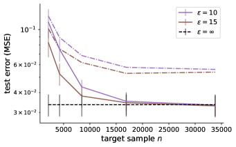
Figure 2: MSE on the Gas dataset over ten runs against the number of target samples with various values of $\epsilon$. Comparison of our algorithm (solid lines) with the noisy minibatch SGD from (Bassily et al., 2019) (dash-dotted lines).

For reference, we also compared our algorithm with the noisy minibatch SGD from (Bassily et al., 2019) (top dash-dotted plots in the figure), see Figure 2. We verify that our algorithm outperforms that noisy minibatch SGD algorithm, which only benefits from the target labeled data.

Table 5: MSE of private adaptation algorithm $\mathsf{CnvxAdap}$ against the non-private DM algorithm on the multi-domain sentiment analysis dataset.

Source	Target	$\mathsf{CnvxAdap}$ ($\varepsilon=4$)	$\mathsf{CnvxAdap}$ ($\varepsilon=10$)	DM
	BOOKS	$1.649\pm 1.909$	$0.713\pm 0.625$	$0.778\pm 0.459$
KITCHEN	DVD	$0.832\pm 0.640$	$0.521\pm 0.354$	$1.396\pm 1.145$
	ELEC	$0.790\pm 0.153$	$0.555\pm 0.139$	$1.740\pm 1.483$
	DVD	$0.929\pm 0.365$	$0.637\pm 0.297$	$0.761\pm 0.562$
BOOKS	ELEC	$0.708\pm 0.092$	$0.485\pm 0.147$	$0.711\pm 0.320$
	KITCHEN	$0.796\pm 0.126$	$0.632\pm 0.181$	$0.956\pm 0.442$
	ELEC	$0.671\pm 0.120$	$0.429\pm 0.189$	$0.677\pm 0.231$
DVD	KITCHEN	$0.665\pm 0.197$	$0.453\pm 0.189$	$1.185\pm 0.753$
	BOOKS	$0.727\pm 0.288$	$0.430\pm 0.143$	$0.676\pm 0.812$
	KITCHEN	$0.671\pm 0.161$	$0.439\pm 0.141$	$1.389\pm 0.755$
ELEC	BOOKS	$0.743\pm 0.365$	$0.351\pm 0.204$	$0.884\pm 0.639$
	DVD	$0.755\pm 0.585$	$0.589\pm 0.495$	$0.843\pm 0.403$

To further illustrate the effectiveness of our algorithms, we also report a series of additional empirical results comparing our private adaptation algorithm $\mathsf{CnvxAdap}$ to the non-private baseline, the DM algorithm (Cortes and Mohri, 2014), on the multi-domain sentiment analysis dataset (Blitzer et al., 2007) formed as a regression task for each category as in prior work Awasthi et al. (2024). We consider four categories: BOOKS, DVD, ELECTRONICS, and KITCHEN. We report MeanSquaredErrors, MSE, for 12 pairwise experiments (TaskA, TaskB) in Table 5. As a source, we use a combination of 500 examples from TaskA and 200 examples from TaskB. For the target data we use 300 examples from TaskB. We use 50 examples from TaskB for validation and 1000 examples for testing. The results are averaged over 10 independent source/target splits, which show that our private adaptation algorithm $\mathsf{CnvxAdap}$ consistently outperforms DM (non-private algorithm), even for $\varepsilon=10$ for this relatively small target sample size.

For a more fair comparison with private-DM (Bassily et al., 2022), here, we also provide results for our private algorithm $\mathsf{CnvxAdap}$ with $\alpha=1$. In future work we seek to estimate $\alpha$ in a principled way based on the discrepancy. Figure 3 shows that even for high values of $n$, the private-DM does not outperform our algorithm.

Hyperparameter tuning

While our algorithm involves hyperparameters, it is important to note that this holds for virtually all standard learning algorithms, even in the absence of adaptation; e.g., neural networks require fine-tuning of multiple parameters through validation datasets. In particular, our methodology does not rely more on hyperparameter tuning than the baselines. Empirical hyperparameter tuning can incur a privacy cost indeed, which requires careful attention. One approach to mitigate this is using privacy-preserving hyperparameter tuning via local sensitivity analysis to estimate the privacy cost of each tuning query.

Sampling with replacement

We use sampling with replacement to increase the number of samples in the datasets we experiment on and enable reporting results for larger values of target sample size $n$. In terms of the privacy guarantee, we would like to note that the sampling with replacement we perform does not mean that each individual in the resulting dataset contributes multiple data points. Each of the repeated data points is viewed as belonging to a different individual (that is, we assume the total number of individuals in the dataset also increases with sampling so that the size of the sampled dataset equals the total number of individuals).

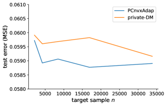
Figure 3: Mean values of MSE on the Gas dataset over ten runs against the number of target samples with $\epsilon=15$. Comparison of our algorithm ($\alpha=1$) with the private-DM from (Bassily et al., 2022).

E.2 Non-convex setting

For the Adult dataset, also known as the Census Income dataset, the source and target data are divided by the gender attribute to predict whether the income exceeds $\$50$K. The source and target data of the South German Credit dataset, German, are divided based on whether the debtor has lived in the present residence for at least three years. The goal is to predict the status of the debtor’s checking account with the bank. The Speaker Accent Recognition dataset, Accent, uses features from the soundtrack of words read by speakers from different countries to predict the accent. The source contains examples whose language attribute is US or UK while the target contains the remaining examples.

We use the CLIP (Radford et al., 2021) model to extract features from the ImageNet (Deng et al., 2009) dataset and extract features from the CIFAR-100, CIFAR-10 (Krizhevsky, 2009) and SVHN (Netzer et al., 2011) datasets by using the outputs of the second-to-last layer of ResNet (He et al., 2016). We transform those datasets into binary classification by assigning half of the labels as $+1$ and the other half as $-1$ and then convert them into domain adaptation tasks where the source and target data consist of distinct mixtures of uniform sampling and Gaussian sampling using the mean and covariance of the data. For the CIFAR-100 and ImageNet datasets, $95\%$ of the source data and $5\%$ of the target data come from Gaussian sampling; for the CIFAR-10 dataset, $90\%$ of the source data and $10\%$ of the target data come from Gaussian sampling; for the SVHN dataset, $80\%$ of the source data and $20\%$ of the target data come from Gaussian sampling.

Appendix F Extensions

Reverse scenario. Notably, given the form of the learning bound and the objective function adopted in our private optimization-based adaptation algorithms, they can be straightforwardly modified to derive private algorithms with similar guarantees in the reverse scenario where the source domain is private while the target domain is public.

Different feature spaces. Our current formulation assumes the same input space for the source and target distributions. For adaptation problems with distinct input feature spaces, two approaches can be taken to extend our results: (1) If the mapping $\Psi$ between the spaces is known, our theory can be readily extended to accommodate this situation. In this case, the adaptation algorithm can be adjusted by incorporating the mapping $\Psi$ in the learning process; we consider $(h\circ\Psi)(x)$ for source domain instances; (2) If the mapping $\Psi$ is unknown, it needs to be learned simultaneously with $h$. In this scenario, we consider $(h\circ\Psi)(x)$ for source domain instances, with $\Psi$ being an integral part of the learning process. We leave a detailed analysis, including a needed extension of the generalization bound of Theorem B.1, to future work. The case of distinct output spaces is similar.

References

- Abadi et al. (2016) Martin Abadi, Andy Chu, Ian Goodfellow, H Brendan McMahan, Ilya Mironov, Kunal Talwar, and Li Zhang. Deep learning with differential privacy. In Proceedings of the 2016 ACM SIGSAC conference on computer and communications security, pages 308–318, 2016.
- Alon et al. (2019) Noga Alon, Raef Bassily, and Shay Moran. Limits of private learning with access to public data. NeuRIPS 2019, also available at arXiv:1910.11519 [cs.LG], 2019.
- Arjevani et al. (2019) Yossi Arjevani, Yair Carmon, John C. Duchi, Dylan J. Foster, Nathan Srebro, and Blake Woodworth. Lower bounds for non-convex stochastic optimization, 2019.
- Awasthi et al. (2024) Pranjal Awasthi, Corinna Cortes, and Mehryar Mohri. Best-effort adaptation. Annals of Mathematics and Artificial Intelligence, to appear, 2024.
- Bassily et al. (2014) Raef Bassily, Adam Smith, and Abhradeep Thakurta. Private empirical risk minimization: Efficient algorithms and tight error bounds. In 2014 IEEE 55th annual symposium on foundations of computer science, pages 464–473. IEEE, 2014.
- Bassily et al. (2018) Raef Bassily, Abhradeep Thakurta, and Om Thakkar. Model-agnostic private learning. In Advances in Neural Information Processing Systems 31, pages 7102–7112. Curran Associates, Inc., 2018.
- Bassily et al. (2019) Raef Bassily, Vitaly Feldman, Kunal Talwar, and Abhradeep Guha Thakurta. Private stochastic convex optimization with optimal rates. Advances in neural information processing systems, 32, 2019.
- Bassily et al. (2020) Raef Bassily, Albert Cheu, Shay Moran, Aleksandar Nikolov, Jonathan Ullman, and Steven Wu. Private query release assisted by public data. In International Conference on Machine Learning, pages 695–703. PMLR, 2020.
- Bassily et al. (2022) Raef Bassily, Mehryar Mohri, and Ananda Theertha Suresh. Private domain adaptation from a public source. CoRR, abs/2208.06135, 2022.
- Beck (2017) Amir Beck. First-order methods in optimization. SIAM, 2017.
- Beimel et al. (2013) Amos Beimel, Kobbi Nissim, and Uri Stemmer. Private learning and sanitization: Pure vs. approximate differential privacy. In Approximation, Randomization, and Combinatorial Optimization. Algorithms and Techniques, pages 363–378. Springer, 2013.
- Ben-David et al. (2010) Shai Ben-David, John Blitzer, Koby Crammer, Alex Kulesza, Fernando Pereira, and Jennifer Wortman Vaughan. A theory of learning from different domains. Machine learning, 79(1-2):151–175, 2010.
- Ben-David et al. (2023) Shai Ben-David, Alex Bie, Clément L. Canonne, Gautam Kamath, and Vikrant Singhal. Private distribution learning with public data: The view from sample compression. CoRR, abs/2308.06239, 2023.
- Bie et al. (2022) Alex Bie, Gautam Kamath, and Vikrant Singhal. Private estimation with public data. In Sanmi Koyejo, S. Mohamed, A. Agarwal, Danielle Belgrave, K. Cho, and A. Oh, editors, Advances in Neural Information Processing Systems 35: Annual Conference on Neural Information Processing Systems 2022, NeurIPS 2022, New Orleans, LA, USA, November 28 - December 9, 2022, 2022.
- Blitzer et al. (2007) John Blitzer, Mark Dredze, and Fernando Pereira. Biographies, bollywood, boom-boxes and blenders: Domain adaptation for sentiment classification. In Proceedings of ACL, pages 440–447, 2007.
- Blitzer et al. (2008) John Blitzer, Koby Crammer, Alex Kulesza, Fernando Pereira, and Jennifer Wortman. Learning bounds for domain adaptation. In Proceedings of NIPS, pages 129–136, 2008.
- Boyd and Vandenberghe (2014) Stephen P. Boyd and Lieven Vandenberghe. Convex Optimization. Cambridge University Press, 2014.
- Chaudhuri and Hsu (2011) Kamalika Chaudhuri and Daniel Hsu. Sample complexity bounds for differentially private learning. In Proceedings of the 24th Annual Conference on Learning Theory, pages 155–186, 2011.
- Cortes and Mohri (2011) Corinna Cortes and Mehryar Mohri. Domain adaptation in regression. In Proceedings of ALT, pages 308–323, 2011.
- Cortes and Mohri (2014) Corinna Cortes and Mehryar Mohri. Domain adaptation and sample bias correction theory and algorithm for regression. Theor. Comput. Sci., 519:103–126, 2014.
- Cortes et al. (2010) Corinna Cortes, Yishay Mansour, and Mehryar Mohri. Learning bounds for importance weighting. In Proceedings of NIPS, pages 442–450. Curran Associates, Inc., 2010.
- Cortes et al. (2019) Corinna Cortes, Mehryar Mohri, and Andrés Muñoz Medina. Adaptation based on generalized discrepancy. J. Mach. Learn. Res., 20:1:1–1:30, 2019.
- de Mathelin et al. (2021) Antoine de Mathelin, Mathilde Mougeot, and Nicolas Vayatis. Discrepancy-based active learning for domain adaptation. CoRR, abs/2103.03757, 2021.
- Deng et al. (2009) Jia Deng, Wei Dong, Richard Socher, Li-Jia Li, Kai Li, and Fei-Fei Li. Imagenet: A large-scale hierarchical image database. In 2009 IEEE conference on computer vision and pattern recognition, pages 248–255. Ieee, 2009.
- Dua and Graff (2017) Dheeru Dua and Casey Graff. UCI machine learning repository, 2017. URL http://archive.ics.uci.edu/ml.
- Dwork and Roth (2014a) Cynthia Dwork and Aaron Roth. The algorithmic foundations of differential privacy. Foundations and Trends® in Theoretical Computer Science, 9(3–4):211–407, 2014a.
- Dwork and Roth (2014b) Cynthia Dwork and Aaron Roth. The algorithmic foundations of differential privacy. Found. Trends Theor. Comput. Sci., 9(3-4):211–407, 2014b.
- Dwork et al. (2006a) Cynthia Dwork, Krishnaram Kenthapadi, Frank McSherry, Ilya Mironov, and Moni Naor. Our data, ourselves: Privacy via distributed noise generation. In Annual International Conference on the Theory and Applications of Cryptographic Techniques, pages 486–503. Springer, 2006a.
- Dwork et al. (2006b) Cynthia Dwork, Frank McSherry, Kobbi Nissim, and Adam D. Smith. Calibrating noise to sensitivity in private data analysis. In Proceedings of Theory of Cryptography Conference TCC, volume 3876 of Lecture Notes in Computer Science, pages 265–284. Springer, 2006b.
- Fernandes (2015) Kelwin Fernandes. A proactive intelligent decision support system for predicting the popularity of online news. In Springer Science and Business Media LLC‘<, 08 2015.
- Germain et al. (2013) Pascal Germain, Amaury Habrard, François Laviolette, and Emilie Morvant. A PAC-bayesian approach for domain adaptation with specialization to linear classifiers. In Proceedings of ICML, volume 28 of JMLR Workshop and Conference Proceedings, pages 738–746. JMLR.org, 2013.
- Ghadimi et al. (2016) Saeed Ghadimi, Guanghui Lan, and Hongchao Zhang. Mini-batch stochastic approximation methods for nonconvex stochastic composite optimization. Mathematical Programming, 155(1):267–305, 2016.
- Graf et al. (2011) F. Graf, H.-P. Kriegel, M. Schubert, S. Poelsterl, and A. Cavallaro. Relative location of CT slices on axial axis. UCI Machine Learning Repository, 2011. DOI: https://doi.org/10.24432/C5CP6G.
- Hanneke and Kpotufe (2019) Steve Hanneke and Samory Kpotufe. On the value of target data in transfer learning. In Hanna M. Wallach, Hugo Larochelle, Alina Beygelzimer, Florence d’Alché-Buc, Emily B. Fox, and Roman Garnett, editors, Advances in Neural Information Processing Systems 32: Annual Conference on Neural Information Processing Systems 2019, NeurIPS 2019, December 8-14, 2019, Vancouver, BC, Canada, pages 9867–9877, 2019.
- Haslett and Raftery (1989) John Haslett and Adrian E. Raftery. Space-time modeling with long-memory dependence: assessing ireland’s wind-power resource. technical report. Journal of the Royal Statistical Society, 38(1), 1989.
- He et al. (2016) Kaiming He, Xiangyu Zhang, Shaoqing Ren, and Jian Sun. Deep residual learning for image recognition. In Proceedings of the IEEE conference on computer vision and pattern recognition, pages 770–778, 2016.
- Huang et al. (2006) Jiayuan Huang, Alexander J. Smola, Arthur Gretton, Karsten M. Borgwardt, and Bernhard Schölkopf. Correcting sample selection bias by unlabeled data. In NIPS 2006, volume 19, pages 601–608, 2006.
- Ikonomovska (2009) Elena Ikonomovska. Airline dataset. Online, 2009. URL http://kt.ijs.si/elena_ikonomovska/data.html.
- Jin et al. (2021) Kaizhong Jin, Xiang Cheng, Jiaxi Yang, and Kaiyuan Shen. Differentially private correlation alignment for domain adaptation. In IJCAI, volume 21, pages 3649–3655, 2021.
- Kifer et al. (2004) Daniel Kifer, Shai Ben-David, and Johannes Gehrke. Detecting change in data streams. In Proceedings of VLDB, pages 180–191. Morgan Kaufmann, 2004.
- Krizhevsky (2009) Alex Krizhevsky. Learning multiple layers of features from tiny images. Technical report, Toronto University, 2009.
- Ledoux and Talagrand (1991) Michel Ledoux and Michel Talagrand. Probability in Banach Spaces: Isoperimetry and Processes. Springer, New York, 1991.
- Li (2012) Qi Li. Literature survey: domain adaptation algorithms for natural language processing. Department of Computer Science The Graduate Center, The City University of New York, pages 8–10, 2012.
- Li and Li (2018) Zhize Li and Jian Li. A simple proximal stochastic gradient method for nonsmooth nonconvex optimization. Advances in neural information processing systems, 31, 2018.
- Lu et al. (2021) Nan Lu, Tianyi Zhang, Tongtong Fang, Takeshi Teshima, and Masashi Sugiyama. Rethinking importance weighting for transfer learning. CoRR, abs/2112.10157, 2021.
- Mansour et al. (2009) Yishay Mansour, Mehryar Mohri, and Afshin Rostamizadeh. Domain adaptation: Learning bounds and algorithms. In Proceedings of COLT, 2009.
- Mohri and Muñoz Medina (2012) Mehryar Mohri and Andres Muñoz Medina. New analysis and algorithm for learning with drifting distributions. In Proceedings of ALT, volume 7568 of Lecture Notes in Computer Science, pages 124–138. Springer, 2012.
- Mohri et al. (2018) Mehryar Mohri, Afshin Rostamizadeh, and Ameet Talwalkar. Foundations of Machine Learning. MIT Press, second edition, 2018.
- Nandi and Bassily (2020) Anupama Nandi and Raef Bassily. Privately answering classification queries in the agnostic pac model. In Algorithmic Learning Theory, pages 687–703, 2020.
- Netzer et al. (2011) Yuval Netzer, Tao Wang, Adam Coates, Alessandro Bissacco, Bo Wu, and Andrew Y Ng. Reading digits in natural images with unsupervised feature learning. In Advances in Neural Information Processing Systems, 2011.
- Pan and Yang (2009) Sinno Jialin Pan and Qiang Yang. A survey on transfer learning. IEEE Transactions on knowledge and data engineering, 22(10):1345–1359, 2009.
- Radford et al. (2021) Alec Radford, Jong Wook Kim, Chris Hallacy, Aditya Ramesh, Gabriel Goh, Sandhini Agarwal, Girish Sastry, Amanda Askell, Pamela Mishkin, Jack Clark, et al. Learning transferable visual models from natural language supervision. In International conference on machine learning, pages 8748–8763. PMLR, 2021.
- Rodriguez-Lujan et al. (2014) Irene Rodriguez-Lujan, Jordi Fonollosa, Alexander Vergara, Margie Homer, and Ramon Huerta. On the calibration of sensor arrays for pattern recognition using the minimal number of experiments. Chemometrics and Intelligent Laboratory Systems, 130:123–134, 2014. ISSN 0169-7439.
- Shamir (2020) Ohad Shamir. Can we find near-approximately-stationary points of nonsmooth nonconvex functions? arXiv preprint arXiv:2002.11962, 2020.
- Sriperumbudur et al. (2007) Bharath K. Sriperumbudur, David A. Torres, and Gert R. G. Lanckriet. Sparse eigen methods by D.C. programming. In ICML, pages 831–838, 2007.
- Steinke and Ullman (2015) Thomas Steinke and Jonathan Ullman. Between pure and approximate differential privacy. arXiv preprint arXiv:1501.06095, 2015.
- Sugiyama et al. (2007a) Masashi Sugiyama, Matthias Krauledat, and Klaus-Robert Müller. Covariate shift adaptation by importance weighted cross validation. J. Mach. Learn. Res., 8:985–1005, 2007a.
- Sugiyama et al. (2007b) Masashi Sugiyama, Shinichi Nakajima, Hisashi Kashima, Paul von Bünau, and Motoaki Kawanabe. Direct importance estimation with model selection and its application to covariate shift adaptation. In Proceedings of NIPS, pages 1433–1440. Curran Associates, Inc., 2007b.
- Tao and An (1998) Pham Dinh Tao and Le Thi Hoai An. A DC optimization algorithm for solving the trust-region subproblem. SIAM Journal on Optimization, 8(2):476–505, 1998.
- Tramèr et al. (2022) Florian Tramèr, Gautam Kamath, and Nicholas Carlini. Considerations for differentially private learning with large-scale public pretraining. CoRR, abs/2212.06470, 2022.
- Vergara et al. (2012) Alexander Vergara, Shankar Vembu, Tuba Ayhan, Margaret A. Ryan, Margie L. Homer, and Ramón Huerta. Chemical gas sensor drift compensation using classifier ensembles. Sensors and Actuators B: Chemical, 166-167:320–329, 2012. ISSN 0925-4005.
- Wang et al. (2019) Boyu Wang, Jorge A. Mendez, Mingbo Cai, and Eric Eaton. Transfer learning via minimizing the performance gap between domains. In Proceedingz of NeurIPS, pages 10644–10654, 2019.
- Wang and Xu (2019) Di Wang and Jinhui Xu. Differentially private empirical risk minimization with smooth non-convex loss functions: A non-stationary view. In Proceedings of the AAAI Conference on Artificial Intelligence, volume 33, pages 1182–1189, 2019.
- Wang et al. (2017) Di Wang, Minwei Ye, and Jinhui Xu. Differentially private empirical risk minimization revisited: Faster and more general. Advances in Neural Information Processing Systems, 30, 2017.
- Wang and Deng (2018) Mei Wang and Weihong Deng. Deep visual domain adaptation: A survey. Neurocomputing, 312:135–153, 2018.
- Wang et al. (2020) Qian Wang, Zixi Li, Qin Zou, Lingchen Zhao, and Song Wang. Deep domain adaptation with differential privacy. IEEE Transactions on Information Forensics and Security, 15:3093–3106, 2020.
- Yuille and Rangarajan (2003) Alan L. Yuille and Anand Rangarajan. The concave-convex procedure. Neural Computation, 15(4):915–936, 2003.
- Zhang et al. (2020a) Tianyi Zhang, Ikko Yamane, Nan Lu, and Masashi Sugiyama. A one-step approach to covariate shift adaptation. In Proceedings of ACML, volume 129 of Proceedings of Machine Learning Research, pages 65–80. PMLR, 2020a.
- Zhang et al. (2019) Yuchen Zhang, Tianle Liu, Mingsheng Long, and Michael I. Jordan. Bridging theory and algorithm for domain adaptation. In Proceedings of ICML, volume 97 of Proceedings of Machine Learning Research, pages 7404–7413. PMLR, 2019.
- Zhang et al. (2020b) Yuchen Zhang, Mingsheng Long, Jianmin Wang, and Michael I. Jordan. On localized discrepancy for domain adaptation. CoRR, abs/2008.06242, 2020b.