Probabilistic-based Feature Embedding of 4-D Light Fields for Compressive Imaging and Denoising

Abstract

The high-dimensional nature of the 4-D light field (LF) poses great challenges in achieving efficient and effective feature embedding, that severely impacts the performance of downstream tasks. To tackle this crucial issue, in contrast to existing methods with empirically-designed architectures, we propose a probabilistic-based feature embedding (PFE), which learns a feature embedding architecture by assembling various low-dimensional convolution patterns in a probability space for fully capturing spatial-angular information. Building upon the proposed PFE, we then leverage the intrinsic linear imaging model of the coded aperture camera to construct a cycle-consistent 4-D LF reconstruction network from coded measurements. Moreover, we incorporate PFE into an iterative optimization framework for 4-D LF denoising. Our extensive experiments demonstrate the significant superiority of our methods on both real-world and synthetic 4-D LF images, both quantitatively and qualitatively, when compared with state-of-the-art methods. The source code will be publicly available at https://github.com/lyuxianqiang/LFCA-CR-NET.

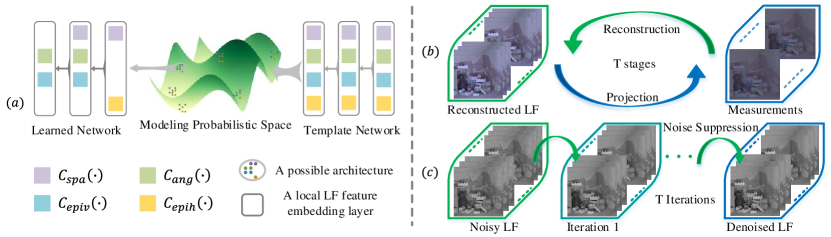
Figure 1: (a) Illustration of probabilistic-based feature embedding. The learned network is derived from the MAP estimation in a probability space using a template network that comprises multiple layers of basic convolution of LF slices, including spatial, angular, vertical EPI, and horizontal EPI slices. Building upon this module, a cycle-consistent framework (b) has been devised for compressive imaging, which involves several iterative stages of projection and reconstruction. During the projection phase, the coded aperture imaging process is simulated. Additionally, we propose an iterative denoising framework (c) comprising multiple iterative noise suppression modules.

1 Introduction

The 4-D light field (LF) records both the spatial and angular information of light rays emanating from the 3-D scene. Owing to its ability to capture richer information, the LF has found applications in various fields, such as digital refocusing Ng et al. (2005, 2006), depth estimation Wanner and Goldluecke (2013); Wang et al. (2015); Park et al. (2017); Jin and Hou (2022), saliency detection Li et al. (2014); Wang et al. (2019); Jing et al. (2021), object recognition Wang et al. (2016), and segmentation Hog et al. (2016). However, this high-dimensional nature of LF data also presents new challenges, particularly in efficiently and effectively extracting its information and features for diverse applications.

To process the 4-D LF, previous learning-based methods simply apply 2-D or 3-D convolutional filters to the stack of sub-aperture images (SAIs) Inagaki et al. (2018); Vadathya et al. (2020); Shin et al. (2018); Zhang et al. (2019), which has a limited ability to explore the angular relations among SAIs. Some advanced network architectures have been designed to model the LF structure better, such as the 4-D convolutional layer Yeung et al. (2019), the epipolar plane images (EPIs) convolutional layer Wu et al. (2017, 2019); Heber et al. (2017), the spatial-angular separable (SAS) convolutional layer Yeung et al. (2018); Jin et al. (2020a); Guo et al. (2020); Jin et al. (2022), the spatial-angular interactive network Wang et al. (2020), the angular deformable convolution Wang et al. (2021a), and the disentangle convolution on macro-pixel image Wang et al. (2023a). However, as these methods combine the spatial and angular features of the LF data in an intuitive or empirical manner, the optimal strategy to model the LF data still needs to be studied. Inspired by the recent advances of Transformer, several Transformer-based methods Wang et al. (2022); Liang et al. (2022, 2023) have been proposed for many LF processing tasks, which can incorporate the information from all angular views and capture long-range spatial dependencies in each SAI.

In this paper, to embed 4-D LF data efficiently and effectively, we propose a probabilistic-based feature embedding module. As shown in Fig. 1, we formulate the problem in a probability space and propose to approximate a maximum posterior distribution (MAP) of a set of carefully defined LF processing events, including both layer-wise spatial-angular feature extraction and network-level feature aggregation. Through droppath from a densely-connected template network, we derive an adaptively probabilistic-based feature embedding, which is sharply contrasted with existing manners that combine spatial and angular features empirically. Building upon the proposed probabilistic-based feature embedding method, we propose two distinct frameworks for the essential tasks of compressive LF imaging and LF image denoising. These tasks are critical in the context of LF data transmission and preprocessing for subsequent applications.

Earlier 4-D LF capturing devices, such as camera array Wilburn et al. (2005) and camera gantry Vaibhav and Andrew , are bulky and costly to capture dense LFs. Although more recent commercial LF cameras, such as Lytro (2016) and RayTrix , are more convenient and efficient, the limited sensor resolution results in a trade-off between spatial and angular resolution. Various manners have been proposed to obtain high-quality 4-D LFs (i.e., 4-D LFs with both high spatial and angular resolution), such as spatial super-resolution Wang et al. (2021a); Jin et al. (2020a); Wang et al. (2023a); Van Duong et al. (2023); Wang et al. (2023b), angular super-resolution (or view synthesis) Jin et al. (2022); Chen et al. (2022); Yang et al. (2023), hybrid lenses Wang et al. (2017); Jin et al. (2023), and coded aperture imaging Inagaki et al. (2018); Vadathya et al. (2020); Guo et al. (2022). Particularly, coded aperture imaging, which encodes the 4-D LF to 2-D coded measurements (CMs) without losing the spatial resolution, demonstrates to be a promising way for high-quality 4-D LF acquisition Wilburn et al. (2005). However, the bottleneck of this manner lies in the ability of the subsequent reconstruction algorithm, which reconstructs the 4-D LF image from the 2-D CMs. Although existing deep learning-based 4-D LF reconstruction methods from CMs Inagaki et al. (2018); Vadathya et al. (2020) have presented significantly better reconstruction quality than conventional ones Babacan et al. (2012); Marwah et al. (2013), they generally employ plain convolutional networks that are purely data-driven without taking the observation model into account. More recently, Guo et al. (2020) proposed an unrolling-based method to link the observation model of coded apertures and deep learning elegantly and improve the LF reconstruction quality significantly. In this paper, we propose a physically interpretable framework incorporated with the probabilistic-based feature embedding to reconstruct the 4-D LF from 2-D CMs. Specifically, based on the intrinsic linear property of the observation model, we propose a cycle-consistent reconstruction network (CR-Net), which reconstructs the LF in a progressive manner by gradually eliminating the residuals between the back-projected CMs from the reconstructed LF and input CMs.

Furthermore, we exploit the probabilistic-based feature embedding approach in the context of LF denoising, which is a fundamental and pressing task for various subsequent LF applications, including but not limited to depth estimation, object recognition, and low light enhancement Lamba et al. (2020). Similar to conventional 2-D images, noise such as thermal and shot noise can corrupt the captured LF data during the acquisition process. However, the higher dimensionality and unique geometric structures of LF data present significant challenges for extending existing low-dimensional signal denoising methods, e.g., 2-D single image denoiser Zhang et al. (2017) or 3-D video denoiser Tassano et al. (2020), to the 4-D LF domain. The state-of-the-art deep learning-based method Guo et al. (2022) considered the LF denoising as a special case of coded aperture LF imaging with the degradation matrix being an identity matrix. The extended pipeline to LF denoising does not fully exploit the characteristics of LF denoising. By sampling analysis for LF noise suppression, we propose an iterative optimization framework for LF denoising with a carefully designed noise suppression module, in which the high-dimensional characteristic of LF denoising can be thoroughly explored. Experimental results demonstrate that the proposed methods outperform state-of-the-art methods to a significant extent.

In summary, the main contributions of this paper are three-fold:

• a probabilistic-based feature embedding method for 4-D LFs;

• a novel framework for coded aperture-based 4-D LF reconstruction; and

• a novel denoising framework for 4-D LF images.

The rest of this paper is organized as follows. Section 2 reviews related works. Section 3 presents the proposed probabilistic-based feature embedding. In Section 4, we present the cycle-consistent network for compressive 4-D LF imaging. In Section 5, we present the iterative optimization network for 4-D LF denoising. In Section 6, extensive experiments are carried out to evaluate our framework on LF coded aperture imaging, and LF denoising. Finally, Section 7 concludes this paper.

Table 1: Summary of feature extraction strategies used for learning-based LF spatial super-resolution, LF angular super-resolution (or view synthesis), coded aperture-based compressive imaging for LF reconstruction, and LF denoising.

Task	Method	Feature Embedding	Processing 4-D information
Spatial Super-resolution	Yoon et al. (2015)	2-D Conv + SAI stacks	No
	Chen et al. (2022)	4-D EPI + PSAIB	Yes
	Wang et al. (2020)	SAS Interaction	Yes
	Wang et al. (2021a)	Angular Deformable Conv	Yes
	Wang et al. (2023a)	2-D Disentangling Conv	Yes
	Van Duong et al. (2023)	2-D Conv + HFEM	Yes
	Wang et al. (2022)	SAS + Transformer	Yes
	Liang et al. (2022)	SAS + Transformer	Yes
	Liang et al. (2023)	SA Correlation + Transformer	Yes
Angular Super-resolution	Wu et al. (2017)	2-D Conv + EPI stacks	No
	Wang et al. (2018)	3-D Conv + EPI stacks	No
	Yeung et al. (2018)	SAS Conv	Yes
	Jin et al. (2020b)	SAS Conv	Yes
	Jin et al. (2022)	SAS Conv	Yes
	Chen et al. (2022)	4-D EPI + PSAIB	Yes
	Wang et al. (2023a)	2-D Disentangling Conv	Yes
	Van Duong et al. (2023)	2-D Conv + HFEM	Yes
	Yang et al. (2023)	4-D Conv + 4-D Deconv	Yes
Compressive Reconstruction	Gupta et al. (2017)	4-D Conv + MLP	Yes
	Inagaki et al. (2018)	2-D Conv + CMs	No
	Vadathya et al. (2020)	2-D Conv + CMs	No
	Guo et al. (2022)	SAS Conv	Yes
Denoising	Chen et al. (2018a)	2-D Conv + SAI stacks	No
	Guo et al. (2022)	SAS Conv	Yes
	Wang et al. (2023c)	2-D Conv + SAI stacks	No

2 Related Work

2.1 Feature Embedding of 4-D LFs

Effective and efficient feature embedding constitutes a fundamental module of diverse learning-based LF tasks and bears a direct relationship to the ultimate performance of the model. Table 1 enumerates the feature extraction techniques utilized in various associated LF tasks, thereby facilitating an intuitive comprehension of the evolution of feature extraction methodologies. Some methods process the 4-D LF from its low-dimensional representation, i.e., 2-D SAI Yoon et al. (2015); Chen et al. (2018a); Wang et al. (2023c), 2-D CMs Inagaki et al. (2018); Vadathya et al. (2020), 2-D EPI Wu et al. (2017), and 3-D EPI Wang et al. (2018) volume, which cannot comprehensively explore the distribution of the high-dimensional data. To comprehensively explore the characteristics of high-dimensional LF, Gupta et al. (2017) employed 4-D convolution and MLP to process the 4-D data. Additionally, Yang et al. (2023) devised LF-ResBlock, which is made up of 4-D convolution and deconvolution, to facilitate angular super-resolution. In addition to this simple idea, Yeung et al. (2018) proposed the SAS convolutional layer that can efficiently process the 4-D LF by sequentially conducting 2-D spatial and angular convolutions. This SAS convolutional layer was employed in several LF tasks, such as angular super-resolution Jin et al. (2022), compressive reconstruction Guo et al. (2020), and LF denoising Guo et al. (2022). Chen et al. (2022) extended the SAS convolutional to parallel spatial-angular integration blocks (PSAIBs), achieving dense interaction between the spatial and angular domain in a two-stream fashion. Wang et al. (2023a) proposed a disentangling mechanism in the 2-D macro-pixel image to extract spatial, angular, and EPI features. However, the empirical combination of spatial, angular, and EPI features may limit the quality of LF reconstruction. Thus, several methods are proposed to combine the high-dimensional feature in some smarter ways Lyu et al. (2021); Van Duong et al. (2023). For example, Van Duong et al. (2023) employed a hybrid feature extraction module (HFEM) that operates on all three 2-D subspaces (i.e., spatial, angular, and EPI) of the LF image. Besides these CNN-based methods, many Transformer-based methods Wang et al. (2022); Liang et al. (2022, 2023) have been proposed for different LF processing tasks.

2.2 Coded Aperture-based 4-D LF Reconstruction

Many conventional methods Liang et al. (2008); Ashok and Neifeld (2010); Babacan et al. (2012); Marwah et al. (2013) have been proposed to reconstruct the LF from CMs. Liang et al. (2008) proposed a method to reconstruct the LF from CMs captured by the programmable aperture system. However, the method requires that the number of measurements is equal to the angular resolution of the reconstructed LF. Ashok and Neifeld (2010) and Babacan et al. (2012) made efforts to reduce the number of required measurements by exploiting the spatial-angular correlations, and employing the hierarchical Bayesian model, respectively. Marwah et al. (2013) proposed an LF reconstruction method through the perspective of compressive sensing that can recover the LF from a single CM by the trained overcomplete dictionary. Limited by the representation ability of the conventional mathematical models and the overcomplete dictionary, the quality of reconstructed LFs of these methods is very limited. With the popularization of deep learning, several deep learning-based methods have been proposed for CM-based LF reconstruction. Gupta et al. (2017) presented a two-branch network for compressive LF reconstruction. Inagaki et al. (2018) used the auto-encoder architecture to encode and decode the LF in an end-to-end manner. However, the LF reconstruction module in these methods is designed from a data-driven perspective and suffers from limited LF reconstruction quality. Vadathya et al. (2020) proposed to estimate disparity maps from CMs and the predicted central SAI, and then warp the central SAI to other ones by using these disparity maps. The performance of this method is affected by the accuracy of the disparity estimation. Guo et al. (2020) proposed a deep unrolling-based method to reconstruct the LF from CMs in a more interpretable way, which significantly improves the LF reconstruction quality.

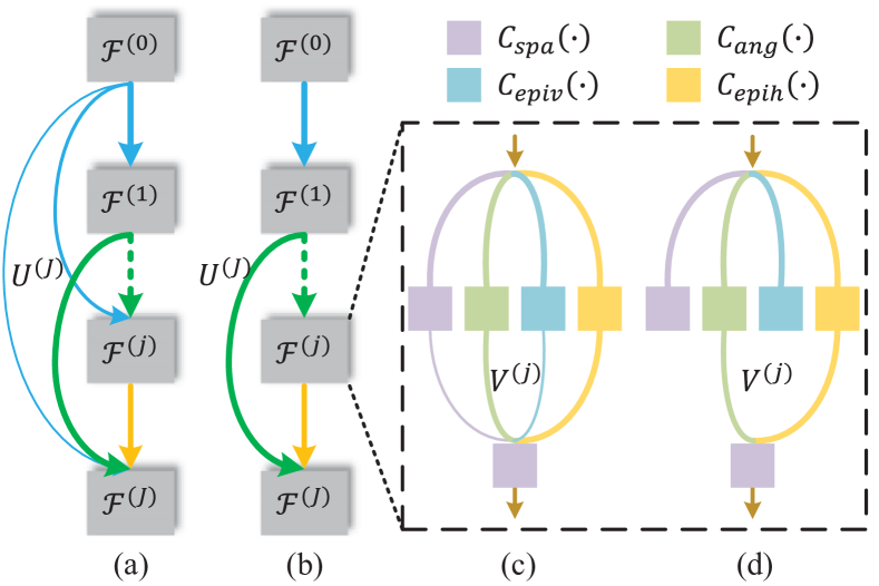
Figure 2: Illustration of network-level feature aggregation and feature embedding unit used in our network. (a,c) The network with all potential paths, namely the template network. (b,d) One possible architecture from the posterior distribution $\mathcal{Q}(\mathcal{W}|\mathbb{D})$.

2.3 4-D LF Image Denoising

Since an LF can be represented as a 2-D array of 2-D images, some conventional methods extend image or video denoising algorithms to LFs. For example, the LFBM5D filter Alain and Smolic (2017) extended the image denoiser BM3D Dabov et al. (2007) to 5-D patches by considering the redundancies in the 2-D angular patch of the LF. In Li et al. (2013), a two-stage framework was proposed to separately suppress the noise of horizontal and vertical EPIs by employing an image denoiser proposed in Beck and Teboulle (2009). Furthermore, Sepas-Moghaddam et al. (2016) utilized the video denoiser Maggioni et al. (2012) to process EPI sequences. From a frequency domain perspective, conducting filtering is an efficient way to segregate the LF signal from noise. Dansereau et al. (2013) explored the characteristics of LFs in the spatial frequency domain and utilized the 4-D hyperfan filter to accomplish LF denoising. In Premaratne et al. (2020), a real-time LF denoising method was proposed using a novel 4-D hyperfan filter, which is approximated in the 4-D mixed-domain using a 2-D circular filter and 2-D parallelogram filters. More recently, Tomita et al. (2022) proposed a denoising method for multi-view images based on the short-time discrete Fourier transform (ST-DFT). The proposed denoising method first transforms noisy multi-view images into the ST-DFT domain, and then noisy ST-DFT coefficients are denoised by soft thresholding derived from the proposed multi-block Laplacian model.

Recently, some deep learning-based LF denoising methods were proposed, which denoise the LF by training with a large amount of LF data. Chen et al. (2018a) proposed a deep learning-based framework for LF denoising with two sequential CNNs. The first network creates the structural parallax details, and the second restores the view-dependent local energies. In Guo et al. (2022), their deep spatial-angular regularization framework was extended to LF denoising, which implicitly and comprehensively explores the signal distribution based on the observation model of noisy LF images. Wang et al. (2023c) utilized the multiple stream progressive restoration network framework and averaged view stacks to LF denoising. These learning-based methods have demonstrated excellent performance for light field denoising.

3 Proposed Probabilistic-based Feature Embedding

To comprehensively explore the spatial-angular information of 4-D LFs, high-dimensional convolution is an intuitive choice that has demonstrated its effectiveness Wang et al. (2018). However, compared to 2-D convolution, it significantly increases the number of parameters, which may cause overfitting and consume significant computational resources. By analogy with the approximation of a high-dimensional filter with multiple low-dimensional filters in the field of signal processing, some researchers have proposed to apply convolutions separately on the spatial Yoon et al. (2015), angular Yeung et al. (2019), or EPI Wu et al. (2017) domains. However, it is laborious and inconvenient to design an optimal LF feature embedding module manually. Furthermore, the aggregations of different layers also play a crucial role during LF reconstruction. Inspired by the current success of neural architectural search Liu et al. (2019); Wang et al. (2021b), we introduce an adaptive probabilistic-based feature embedding module that builds a probabilistic model to locally choose the LF feature embedding patterns and globally optimize the aggregation patterns of different layers. Thus, both the network architecture and corresponding weights are optimized to achieve efficient and effective LF reconstruction.

To better demonstrate the possible events during LF feature embedding, we first construct the modeling probabilistic space over each probabilistic-based feature embedding module $\mathcal{D}^{(t)}(\cdot)(0\leq t\leq T-1)$. Denote the global probability space of LF-processing CNNs with $\mathcal{W}=\{(\mathbf{U}^{(1)},\mathcal{F}^{(1)})\cdots(\mathbf{U}^{(j)},\mathcal{F}^{(j)})\cdots(\mathbf{U}^{(J)},\mathcal{F}^{(J)})\}$, where a binary vector $\mathbf{U}^{(j)}\in\{\mathbf{0},\mathbf{1}\}^{j-1}$ with length $j-1$ indicates whether the features from previous $j-1$ layers are used, and $\mathcal{F}^{(j)}$ denotes a feature embedding unit to learn high-level LF embeddings. According to the characteristics of LF images, we further introduce four 2-D convolutional patterns for local LF feature embedding, i.e., $\mathcal{F}^{(j)}=\{\mathbf{V}^{(j)},\mathcal{C}_{spa}^{(j)}(\cdot),\mathcal{C}_{ang}^{(j)}(\cdot),\mathcal{C}_{epih}^{(j)}(\cdot),\mathcal{C}_{epiv}^{(j)}(\cdot)\}$, where $\mathcal{C}_{spa}^{(j)}(\cdot)$, $\mathcal{C}_{ang}^{(j)}(\cdot)$, $\mathcal{C}_{epiv}^{(j)}(\cdot)$, and $\mathcal{C}_{epih}^{(j)}(\cdot)$ denote the 2-D convolutional layers on spatial, angular, vertical EPI, and horizontal EPI domains, respectively; $\mathbf{V}^{(j)}\in\{\mathbf{0},\mathbf{1}\}^{4}$ is a binary vector with length of 4 for selecting different convolution patterns. Then we could drive a deep neural network by solving the maximum a posterior (MAP) estimation problem:

$$\widehat{\mathcal{W}}=\mathop{\arg\max}_{\mathcal{W}}\mathcal{Q}\left(\mathcal{W}|\mathbb{D}\right),$$ (1)

where $\mathbb{D}=\{\mathbf{I},\mathbf{L}\}$ indicates the data distributions.

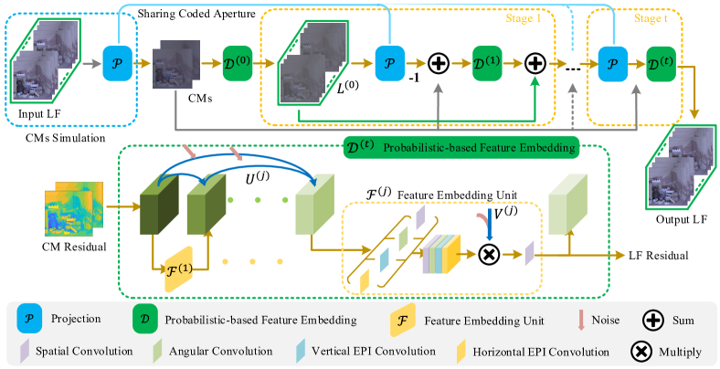
Figure 3: Illustration of the proposed framework named CR-Net for reconstructing 4-D LF images from 2-D measurements by a coded-aperture camera. CR-Net consists of a ”CMs Simulation” procedure and the proposed cycle-consistent reconstruction network.

To solve Eq. (1), we first approximate the posterior distribution $\mathcal{Q}\left(\mathcal{W}|\mathbb{D}\right)$. According to Gal and Ghahramani (2016), embedding dropout into CNNs could objectively minimize the Kullback–Leibler divergence between an approximation distribution and posterior deep Gaussian process Damianou and Lawrence (2013). Thus, we could approximate the posterior distribution via training a template network with binary masks that follow learnable independent Bernoulli distributions (we name the network with all $\mathbf{U}^{(j)}$ and $\mathbf{V}^{(j)}$ set to $\mathbf{1}$ as the template network). As shown in Fig. 2, both the path for feature aggregation ($\mathbf{U}^{(j)}$) and local feature embedding pattern ($\mathbf{V}^{(j)}$) are replaced by masks of logits $\epsilon\sim\mathcal{B}(p)$, where $\mathcal{B}(p)$ denotes the Bernoulli distribution with probability $p$. However, the classical sampling process makes it hard to manage a differentiable linkage between the sampling results and the probability. Besides, such dense aggregations in CNNs result in a huge number of feature embeddings. Thus, we also need to explore an efficient and effective way of aggregating those features masked by binary logits. In what follows, we detailedly discuss those two aspects.

To obtain a differentiable sampling manner of logits $\epsilon$, we use the Gumbel-softmax Jang et al. (2017) to relax the discrete Bernoulli distribution to continuous space. Mathematically, we formulate this process as

$$\small\mathcal{M}(p)=\textsf{Sigmoid}\{ \frac{1}{\tau}(\log p-\log(1-p)+\log(\log({r_{1}}))$$

$$-\log(\log({r_{2}})))\},$$ (2)

where $r_{1}$ and $r_{2}$ are random noises with standard uniform distribution in the range of $[0,1]$; $p$ is a learnable parameter encoding the probability of aggregations in the neural network; $\tau>0$ is a temperature that controls the similarity between $\mathcal{M}(p)$ and $\mathcal{B}(1-p)$, i.e., as $\tau\to 0$, the distribution of $\mathcal{M}(p)$ approaches $\mathcal{B}(1-p)$; while as $\tau\to\infty$, $\mathcal{M}(p)$ becomes a uniform distribution.

To aggregate the features efficiently and effectively, we design the network architecture at both the network and layer levels. According to Eq. (2), we approximate the discrete variable $\mathbf{U}^{(j)}$ by applying Gumbel-softmax $\mathcal{M}(\cdot)$ to continuous learnable variables $\widetilde{\mathbf{U}}^{(j)}$. Thus, we could formulate network-level feature aggregation as

$$\widetilde{\mathbf{H}}^{(j)}={\mathcal{C}_{1\times 1}}\left({{\mathbf{T}^{(0,j)},\cdots,\mathbf{T}^{(j-1,j)}}}\right),$$

$${\rm with}~{}~{}\mathbf{T}^{(k,j)}={\mathbf{H}}^{(k)}\times\mathcal{M}\left(\widetilde{\mathbf{U}}^{(j)}(k)\right),$$ (3)

where $\widetilde{\mathbf{H}}^{(j)}~{}~{}(1\leq j\leq J)$ denotes the aggregated feature which would be fed into $\mathcal{F}^{(j)}$; $\mathbf{H}^{(k)}~{}~{}(1\leq k\leq j-1)$ represents the feature from the ${k}$-th embedding unit $\mathcal{F}^{(k)}$; $\mathbf{H}^{(0)}$ denotes an LF embedding extracted from the input of $\mathcal{D}^{(t)}(\cdot)$ by a single linear convolutional layer; $\widetilde{\mathbf{U}}^{(j)}(k)$ indicates the ${k}$-th element of the vector $\widetilde{\mathbf{U}}^{(j)}$, which is random initialized and kept in a range of $[0,1]$ according to its meaning of the sampling probability of $\mathbf{U}^{(j)}$; and $\mathcal{C}_{1\times 1}(\cdot)$ represents a $1\times 1$ kernel to compress the feature embedding and activate them with $ReLU$.

In analogy to the network level, we also introduce the continuous learnable weights $\widetilde{\mathbf{V}}^{(j)}$ with Gumbel-softmax to approximate the Bernoulli distribution of $\mathbf{V}^{(j)}$ in each feature embedding unit, as

$${\mathbf{H}^{(j+1)}}={\mathcal{C}_{spa}}\left({{{\mathcal{C}}_{1\times 1}}\left(\mathbf{O}^{(1,j)},\cdots,\mathbf{O}^{(4,j)}\right)}\right),$$

$${\rm with}~{}~{}\mathbf{O}^{(l,j)}=\mathcal{C}_{l}^{(j)}\left(\widetilde{\mathbf{H}}^{(j)}\right)\times\mathcal{M}\left(\widetilde{\mathbf{V}}^{(j)}(l)\right),$$ (4)

where $\mathcal{C}_{l}^{(j)}(\cdot)~{}~{}(l\in\{1,2,3,4\})$ indicates the previously designed one of the four convolution patterns in $\mathcal{F}^{(j)}$, which are $\mathcal{C}_{spa}^{(j)}(\cdot)$, $\mathcal{C}_{ang}^{(j)}(\cdot)$, $\mathcal{C}_{epih}^{(j)}(\cdot)$, and $\mathcal{C}_{epiv}^{(j)}(\cdot)$, respectively. After applying a $1\times 1$ convolutional layer to compress the embedding, we adopt a further spatial convolution after fusing the feature from different patterns, due to that spatial convolution plays an essential role during the feature embedding process.

Training such a masked template neural network results in a posterior distribution $\mathcal{Q}(\mathcal{W}|\mathbb{D})$. Meanwhile, through droppath with lower probability, we could finally derive a neural network with maximum posterior probability (see Fig. 12 for the detailed network architecture).

4 Proposed Coded Aperture-based 4-D LF Reconstruction

Problem Statement. Denote by $\mathbf{L}(u,v,x,y)\in\mathbb{R}^{M\times N\times H\times W}$ the 4-D LF, where $\{(u,v)|u\in[1,M],v\in[1,N]\}$ and $\{(x,y)|x\in[1,H],y\in[1,W]\}$ are angular and spatial positions, respectively. Then, the $i$-th 2-D CM, denoted as $\mathbf{I}_{i}\in\mathbb{R}^{H\times W}$, captured by the coded aperture camera can be formulated as:

$$\mathbf{I}_{i}(x,y)=\sum_{u=1}^{M}\sum_{v=1}^{N}a_{i}(u,v)\mathbf{L}(u,v,x,y),\\$$ (5)

where $a_{i}(u,v)\in[0,1]$ is the transmittance at aperture position $(u,v)$ for the $i$-th acquisition. Following Inagaki et al. (2018), we simulate the imaging process in Eq. (5) to make the coded aperture jointly learned with the subsequent reconstruction. Specifically, shown as the ”CMs Simulation” procedure in Fig. 3, we utilize a convolutional layer, denoted as $\mathcal{P}(\cdot)$, with the input of the 4-D LF to generate $S$ CMs, denoted as $\mathbf{I}\in\mathbb{R}^{S\times H\times W}$. To retrieve $\mathbf{L}$ from $\mathbf{I}$ utilizing a deep learning-based methodology that is predicated on probabilistic-based feature embedding, it is imperative to devise an efficient framework that is tailored to the characteristics of LF compressive imaging. This constitutes a crucial concern for compressive LF reconstruction.

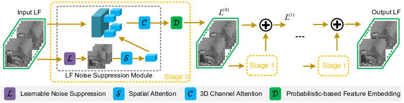
Figure 4: Illustration of the process of the proposed 4-D LF denoising method, namely DN-Net.

Our Solution. The coded aperture model described in Eq. (5) indicates the cycle consistency between the LF and CMs, i.e., a well-reconstructed LF image could be accurately projected to input CMs. Based on this observation, we propose a cycle-consistent reconstruction framework, which progressively refines the reconstructed LF via iteratively projecting the reconstructed LF images to pseudo-CMs, then learning a correction map from the differences between measured CMs and pseudo-CMs. Specifically, as illustrated in Fig. 3, the proposed CR-Net basically consists of two modules, i.e., coarse estimation and cycle-consistent LF refinement.

Coarse Estimation. We first learn a coarse estimation $\mathbf{L}^{(0)}$ of the LF from CMs, expressed as:

$${\mathbf{L}^{(0)}}=\mathcal{D}^{(0)}\left(\mathbf{I}\right),$$ (6)

where $\mathcal{D}^{(0)}(\cdot)$ denotes a probabilistic-based feature embedding module for the coarse LF estimation.

Cycle-consistent LF Refinement. We iteratively learn the LF refinement from the residuals between pseudo-CMs and measured CMs, as:

$${\mathbf{L}^{(t+1)}}=\mathcal{D}^{(t)}\left(\mathbf{I}-\mathcal{P}\left(\mathbf{L}^{(t)}\right)\right)+\mathbf{L}^{(t)},$$ (7)

where $\mathcal{P}(\cdot)$ represents the projection process, which is the same as the convolutional layer used for aperture learning, and $\mathcal{D}^{(t)}(\cdot)(t=1,\cdots,T-1)$ indicates the probabilistic-based feature embedding module for LF refinement. After iteratively refining the LF images, we could get the final LF estimation, denoted as $\mathbf{L}^{(T)}$.

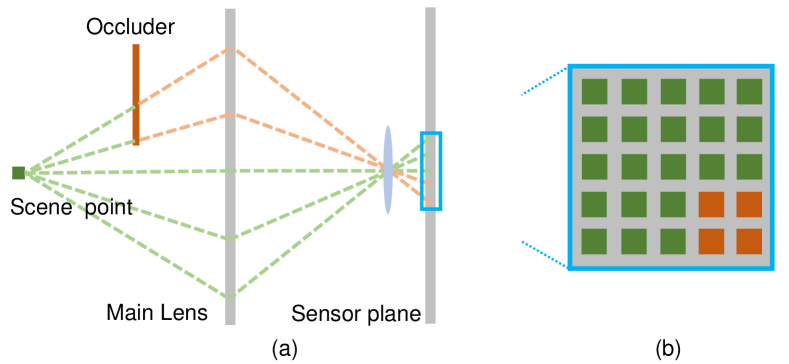
Figure 5: Illustration of imaging model when the occlusion occurs. (a) The imaging process influenced by the occluder. (b) Corresponding angular patch by fixed spatial positions.

5 Proposed 4-D LF Image Denoising

Problem Statement. Let $\mathbf{L}_{noisy}\in\mathbb{R}^{M\times N\times H\times W}$ denote an observed noisy 4-D LF, with an observation model $\mathbf{L}_{noisy}=\mathbf{L}+\mathbf{N}$, where $\mathbf{L}\in\mathbb{R}^{M\times N\times H\times W}$ and $\mathbf{N}\sim\mathcal{N}(\mu,{\sigma^{2}})$ are the noise-free LF and additive white Gaussian noise, respectively. Our objective is to restore $\mathbf{L}$ from $\mathbf{L}_{noisy}$.

Assuming a Lambertian model, the light ray emitted by a target scene is recorded by different SAIs of a 4-D LF from various perspectives, and the light ray’s intensity should be consistent across the SAIs, denoted by $\mathbf{L}_{noisy}^{i}\in\mathbb{R}^{H\times W}$. In the presence of additive white Gaussian noise, the observed light intensity from each SAI conforms to a Gaussian distribution, i.e., $l_{noisy}(u,v,x,y)\sim\mathcal{N}(l(u,v,x,y),{\sigma^{2}})$, where $l_{noisy}$ and $l$ correspond to the intensity of the noisy and noise-free light, respectively. For simplicity, we analyze a group of light rays corresponding to a single scene/object point. As shown in Fig. 5, we obtain a sampling set of light rays in different SAIs, denoted as $l_{noisy}^{all}=\left\{{l_{noisy}^{1},...,l_{noisy}^{Q}}\right\}$, where $Q\leq M\times N$ independent and identically distributed samples. We estimate the noise-free light intensity $l$ using maximum likelihood estimation (MLE) as follows:

$${l_{MLE}}=\frac{1}{Q}\sum\limits_{i=1}^{Q}{l_{noisy}^{i}}$$ (8)

Our Solution. In the presence of occlusions, the number of samples in the sampling set may be less than the angular number, i.e., $Q<M\times N$. Directly applying Eq. (8) to all SAIs can lead to the loss of high-frequency details in the noise suppression result due to occlusion and parallax information. As shown in Fig. 4, we propose an iteratively optimized network for LF denoising. The proposed network leverages probabilistic-based feature embedding and introduces an LF noise suppression module that consists of three particular parts to address the aforementioned blur effect, i.e., learning-based noise suppression, spatial attention for the noise suppression feature, and 3-D channel attention for the combined feature. The subsequent iterative stages predict the residual for denoised LF refinement.

Learning-based Noise Suppression. Extending Eq. (8) to angular averaging of all SAIs can suppress noise and provide guidance for each SAI denoising. However, the occlusion relation can cause high-frequency details to be lost by mixing scene and occluder information. To address this issue, we propose a learning-based noise suppression denoted as $\mathcal{L}(\mathbf{L}_{noisy})$, which concatenates the angular averaging result with seven adaptive angular fusion results.

Spatial Attention for Noise Suppression Feature. The parallax structure of the LF can also result in blurry noise suppression outcomes. Therefore, we incorporated a spatial attention module to process the features of the noise suppression $\mathcal{L}(\mathbf{L}{noisy})$ and reduce the impact of the blurred region. The spatial attention module is defined as follows:

$$\mathcal{F}^{S}=\texttt{SA}(\mathcal{F}(\mathcal{L}(\mathbf{L}_{noisy})))$$ (9)

Here, $\mathcal{F}$ and $\mathcal{F}^{S}$ represent the feature of $\mathcal{L}(\mathbf{L}_{noisy})$ and the output of the spatial attention module, respectively. The function $\texttt{SA}(\cdot)$ denotes the spatial attention processing.

3-D Channel Attention for the Combined Feature. We utilize the feature $\mathcal{F}^{S}$ to guide the LF denoising by concatenating it with each SAI’s feature $\mathcal{F}(\mathbf{L}_{noisy}^{i})$ and then applying 3-D channel attention to filter out the effective channels. This is expressed as:

$$\mathcal{F}^{C}=\texttt{CA}({Cat}_{i=1}^{M\times N}(\mathcal{F}(\mathbf{L}_{noisy}^{i}),\mathcal{F}^{S})$$ (10)

Here, $\texttt{CA}(\cdot)$ represents the 3-D channel attention processing, and $\mathcal{F}^{C}$ denotes the output of the 3-D channel attention module, which is then processed by the subsequent probabilistic-based feature embedding module.

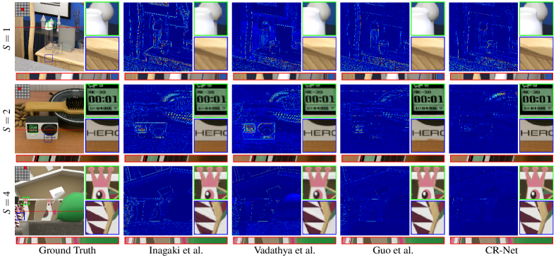
Figure 6: Visual comparisons of reconstructed LFs from different methods under tasks $S=1$, $S=2$, and $S=4$, over the HCI+Inria dataset. The error maps of SAIs and zoomed-selected regions are shown for better visualization.

Table 2: Quantitative comparisons (PSNR/SSIM) of different methods over the test LFs in Lytro and HCI+Inria datasets under three tasks. The number of network parameters (M) of different methods is also provided.

Dataset	Method	S = 1	S = 2	S = 4	# Parameters
Lytro	Inagaki et al. (2018)	32.11/0.910	39.33/0.971	40.17/0.975	0.69
	Vadathya et al. (2020)	35.62/0.964	38.46/0.979	39.27/0.985	5.14
	Guo et al. (2022)	34.39/0.941	41.66/0.984	43.19/0.988	3.33
	CR-Net	34.43/0.938	42.54/0.985	45.18/0.990	1.75
HCI+Inria	Inagaki et al. (2018)	30.60/0.857	34.91/0.934	35.4/0.928	0.69
	Vadathya et al. (2020)	30.82/0.866	32.69/0.925	36.46/0.950	5.14
	Guo et al. (2022)	30.72/0.873	38.55/0.963	42.41/0.976	3.33
	CR-Net	32.17/0.885	42.49/0.973	46.88/0.983	1.75

6 Experiments

6.1 Experiment Settings

Datasets. We conducted experiments on both simulated and real CMs in compressive LF imaging. Specifically, we used the same datasets as those used in Guo et al. (2020) for simulated CMs, which include two LF datasets named Lytro and HCI+Inria. The Lytro dataset consists of $100$ LF images for training and $30$ LF images for testing, which were captured using a Lytro (2016) Illum provided by Kalantari et al. (2016). The HCI+Inria dataset includes $22$ training LF images from the HCI LF dataset Honauer et al. (2016), $33$ training LF images from the Inria Dense LF dataset Shi et al. (2019), $2$ testing LF images from the HCI LF dataset Honauer et al. (2016), and $4$ testing LF images from the Inria Dense LF dataset Honauer et al. (2016). Additionally, we evaluated our method on measurements captured by a real coded aperture camera Inagaki et al. (2018) (details provided in Section 6.2.2).

In LF denoising, we used the same settings as Chen et al. (2018a) for the Stanford Archive dataset, which includes $70$ LF images for training and $30$ LF images for testing. For the HCI+Inria dataset, we used $55$ synthetic LF images of size $7\times 7\times 512\times 512$ for training and $6$ synthetic LF images for testing.

Training Settings. During training, we calculated the $\mathcal{L}_{1}$ distance between $\mathbf{L^{(T)}}$ and the ground-truth LF as the loss function of our network. In the training phase, we randomly cropped the training LF image into patches with size $M\times N\times 32\times 32$. The batch size was set to $5$. The training process consisted of $10K$ pre-training and $10K$ training epochs. We manually set all $\mathbf{U}$ and $\mathbf{V}$ to $1$ for pre-training. In the first $40\%$ training epoch, the value of $\tau$ decreased linearly from 1 to 0.05 and remained unchanged in the follow-up. We chose the Adam optimizer Kingma and Ba (2014) and used OneCycleLR Smith and Topin (2019) to schedule the learning rate. Our network was implemented with PyTorch.

Network Settings. We set $T~{}~{}=6$ and $J~{}~{}=8$ for CR-Net and $T~{}~{}=2$ and $J~{}~{}=6$ for our denoising network (see Sections 6.2.3 and 6.3.5 for the ablation study on the effect of $T$ and $J$). In each $\mathcal{D}^{(t)}(\cdot)~{}~{}(0\leq t\leq T-1)$, the kernel size of four types of convolution methods was set to $3\times 3$, and the output feature channel was set to $32$ and $64$ for CR-Net and DN-Net, respectively. Since $\mathcal{D}^{(t)}(\cdot)$ processes residual information, we removed all biases from the convolutional layers. It’s worth noting that all projection layers $\mathcal{P}(\cdot)$ shared the same weights. Additionally, due to their physical interpretation, all parameters in $\mathcal{P}(\cdot)$ were clipped to the range of $[0,1]$ during the training process.

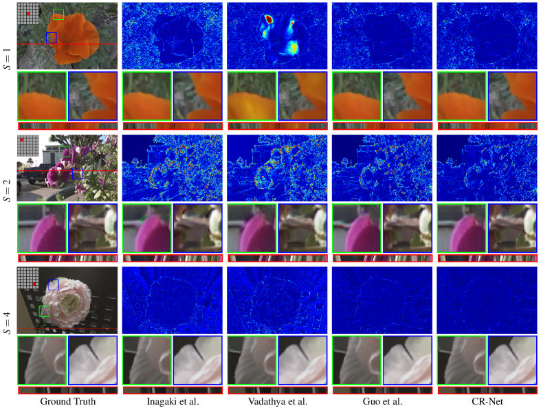
Figure 7: Visual comparisons of reconstructed LFs from different methods under three tasks over the Lytro dataset. The error maps of SAIs and zoomed selected regions are shown for better visualization.

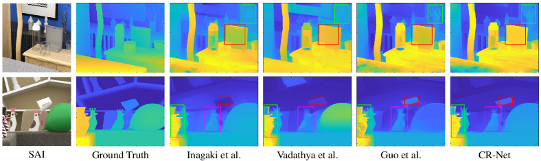
Figure 8: Visual comparisons of ground-truth depth maps and the estimated depth maps from the reconstructed LFs by different methods under task $S=2$ over the HCI+Inria dataset.

6.2 Evaluation on Compressive LF Reconstruction

6.2.1 Comparisons on Simulated CMs

We compared our CR-Net with three state-of-the-art deep learning-based LF reconstruction methods from CMs, i.e., Inagaki et al. (2018), Vadathya et al. (2020), and Guo et al. (2022). For a fair comparison, all methods were re-trained on the same training datasets with officially released codes and recommended configurations. We conducted three tasks on the Lytro dataset, i.e., reconstructing $7\times 7$ LFs with the input measurement number $S=1$, $S=2$, and $S=4$, respectively. We also conducted three tasks on the HCI+Inria dataset, i.e., reconstructing $5\times 5$ LFs with the input measurement number $S=1$, $2$, and $4$, respectively.

Quantitative comparisons. We separately calculated the average PSNR and SSIM over LFs in test datasets to quantitatively compare different methods. The results are shown in Table 2, where it can be observed that:

• CR-Net achieves better performance with a smaller model size than all compared methods on most tasks, which gives credit to our physical interpretable cycle-consistent framework and the probabilistic-based feature embedding strategy;

• Inagaki et al. (2018) has significantly lower PSNR and SSIM values than CR-Net on both Lytro and HCI+Inria datasets. The reason may be that Inagaki et al. (2018) simply employs 2-D convolutional filters that are unable to model the 4-D LF well;

• Vadathya et al. (2020) outperforms CR-Net under task $S=1$ on the Lytro dataset, which may be credited to its explicit use of geometry information. However, our CR-Net achieves much higher PSNR, i.e., about $5$ dB, than Vadathya et al. (2020) under tasks $S=2$ and $S=4$ on the Lytro dataset, because our probabilistic-based feature embedding strategy has the stronger representative ability to model the dimensional correlations among the LF with more than one CMs. Moreover, the proposed CR-Net significantly outperforms Vadathya et al. (2020) under all tasks on the HCI+Inria dataset. We believe the reason is that LFs contained in this dataset have relatively large disparity, resulting in heavily blurred CMs, and thus, Vadathya et al. (2020) could have difficulties predicting a high-quality central SAI for view reconstruction; and

• CR-Net outperforms Guo et al. (2022) on both Lytro and HCI+Inria datasets. The possible reason is that Guo et al. (2022) employs the SAS convolutional layer, which combines spatial and angular dimensions in an empirical manner, while our method can adaptively learn the fusion of the spatial-angular features.

Qualitative comparisons. Fig. 6 and Fig. 7 show visual comparisons of reconstructed LFs from different methods. We can observe that CR-Net produces better visual results than all the compared methods. Specifically, Inagaki et al. (2018) and Vadathya et al. (2020) show blurry effects, and lose high-frequency details at texture regions, while our CR-Net can reconstruct sharp details at both texture and smooth regions. Besides, Guo et al. (2022) shows distortions at occlusion boundaries, while our CR-Net can reconstruct clearer and more accurate structures.

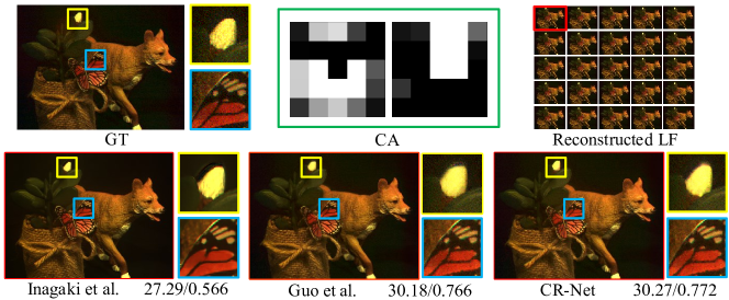
Figure 9: Comparisons of our CR-Net against Inagaki et al. (2018) and Guo et al. (2022) on real CMs. The PSNR/SSIM values are calculated between the reconstructed LF and the pinhole images.

Comparisons of the LF parallax structure. The quality of the parallax structure is one of the most important criteria for evaluating the reconstructed LF. To compare the ability to preserve the LF parallax structure, we visualized EPIs of the reconstructed LFs using different methods. As shown in Fig. 6 and Fig. 7, we observe that the proposed CR-Net shows clearer and sharper linear structures than the compared methods, which demonstrates better preservation of the parallax structures of reconstructed LFs. Moreover, the accuracy of the depth map estimated from the reconstructed LF reflects how well the parallax structure is preserved to some extent. Therefore, we compared the depth maps estimated from different methods using the same depth estimation method Chen et al. (2018b) and the ground truth depth maps. As shown in Fig. 8, we can see that the depth maps of CR-Net are more similar to those of the ground truth at both smooth regions and occlusion boundaries. This means that our method can better preserve the parallax structure than other methods.

6.2.2 Comparisons on Real CMs

To demonstrate the ability of our method on real CMs, we adopted the real data captured by a coded aperture camera built by Inagaki et al. Inagaki et al. (2018). The real data contains $2$ CMs, $2$ masks that are used for capturing the CMs, and the captured $5\times 5$ pinhole images as the ground truth. We fixed the weights of $\mathcal{P}$ to the mask values, and re-trained the CR-Net under the task $S=2$ on the HCI+Inria dataset. Then, we tested the trained model with the real CMs, and compared the reconstructed LF by our CR-Net against that of Inagaki et al. (2018) and Guo et al. (2022). The results are shown in Fig. 9, where it can be observed that the reconstructed LF from our CR-Net is closer to the ground-truth one, while the results from Inagaki et al. (2018) show blurring artifacts at the occlusion boundaries, demonstrating the advantage of our CR-Net on real CMs.

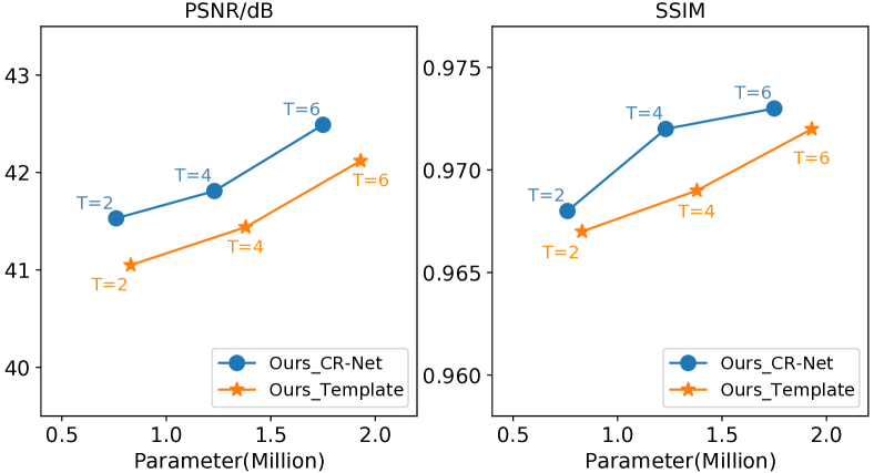
Figure 10: Quantitative results of our final network, denoted as Ours_CR-Net, and the template network without probabilistic modeling, denoted as Ours_Template, under different numbers of stages. The PSNR/SSIM values under the task $S=2$ on the HCI+Inria dataset as well as the model size are provided for comparisons.

6.2.3 Ablation Study

The number of stages and feature embedding units for the CR-Net. To investigate the influence of the number of stages and feature embedding units on the performance, we compared the results of CR-Net using $T=2$, $4$ and $6$ and $J=6$, $8$, and $10$. As demonstrated in Fig. 10 and Table 3, the PSNR/SSIM values gradually improve from $2$ to $6$ stages for our CR-Net and the template network. Moreover, $8$ feature embedding units yield better reconstruction quality. Consequently, for superior LF reconstruction quality, we selected $6$ stages and $8$ feature embedding units in our CR-Net.

Additionally, to further demonstrate the effectiveness of the iterative refinement framework, we visualized the output of each stage of our CR-Net. As shown in Fig. 11, the quality of the reconstructed LF gradually improves from the first stage to the last one, demonstrating the effectiveness of the proposed progressive refinement framework based on the cycle-consistency.

Table 3: Performance comparisons of our CR-Net with different numbers of stages and feature embedding units in a probabilistic-based feature embedding module.

		PSNR	SSIM	# Parameters
$T=6$	$J=6$	41.55	0.968	1.41
	$J=8$	42.49	0.973	1.75
	$J=10$	41.91	0.969	2.48
$J=8$	$T=2$	41.53	0.968	0.82
	$T=4$	41.81	0.972	1.38
	$T=6$	42.49	0.973	1.75

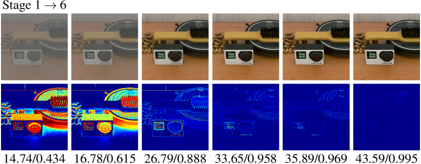
Figure 11: Visualization of the intermediate output at each stage of CR-Net. The first row presents central SAIs of the output LFs, and the second row presents error maps between the reconstructed central SAIs and ground-truth ones. The PSNR/SSIM values of the output LFs at different stages are listed below.

Effectiveness of modeling probabilistic space. In Fig. 12, we visualized the finally learned architecture for the probabilistic-based feature embedding module, where it can be seen that both the layer-wise feature extraction and network-level feature aggregation are adaptively constructed based on the probabilistic modeling. Furthermore, to evaluate the effectiveness of modeling probabilistic space, we quantitatively compared the performance of the final learned CR-Net against the template network. As shown in Fig. 10 and Table 4, it can be observed that the final CR-Net consistently achieves higher performance with a smaller model size compared with the template network under different numbers of stages, which demonstrates the effectiveness of modeling probabilistic space for space-angular fusion in our method.

Effectiveness of the probabilistic-based feature embedding module. To verify the effectiveness of the probabilistic-based feature embedding module $\mathcal{D}(\cdot)$, we replaced $\mathcal{D}(\cdot)$ in each stage with either a stack of 3-D convolution layers or a stack of SAS layers while keeping a comparable model size to our CR-Net. The resulting networks are denoted as CR-Conv3D and CR-SAS, respectively, and their performance was compared with our CR-Net in Table 4. The results indicate that replacing the probabilistic-based feature embedding module with 3-D convolution or SAS layers leads to obvious performance degradation, which further demonstrates the advantage of the proposed probabilistic-based feature embedding strategy.

Effectiveness of sharing weights in projection layers. We also verified the effectiveness of sharing weights of the projection layers across different stages. As shown in Table 4, the performance of the model without sharing the weights of the projection layers, denoted as w/o sharing $\mathcal{P}(\cdot)$, is lower than the CR-Net. The reason is that sharing weights guarantees that the projection layers across all stages correspond to the same physical imaging process. As the pseudo-CMs are produced under the same projection, the residual between the pseudo-CMs and the input CMs is consistent and can be minimized progressively.

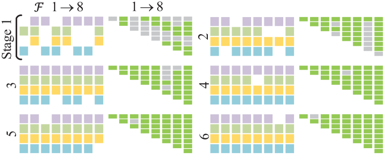
Figure 12: Visualization of the learned architecture for the probabilistic-based feature embedding in the CR-Net for task $S=2$ over the HCI+Inria dataset. The CR-Net contains $6$ stages and $8$ feature embedding units in each stage. For each stage, we show the reserved convolution patterns by patches with different colors on the left, and the network-level feature aggregation results on the right accordingly, where the used features are marked in green.

Table 4: Effectiveness of the probabilistic-based feature embedding module and sharing the weights of projection layers in the proposed CR-Net. The results on task $S=2$ over the HCI+Inria dataset are provided for comparisons.

	PSNR	SSIM	# Parameters
w/o sharing $\mathcal{P}(\cdot)$	41.67	0.970	1.75
CR-Conv3D(1)	40.42	0.963	1.78
CR-Conv3D(2)	41.34	0.966	2.67
CR-SAS	41.11	0.966	1.78
CR-Template	42.12	0.972	1.83
CR-Net	42.49	0.973	1.75

Table 5: Quantitative comparisons (PSNR/SSIM) of different methods over the test LFs in Stanford Archive and HCI+Inria datasets under the denoising task of three noise levels. The number of network parameters (M) of different methods is also provided. “-” indicates that the method is not a deep learning-based method.

Dataset	Method	$\sigma=10$	$\sigma=20$	$\sigma=50$	# Parameters
Stanford Archive	DeamNet Ren et al. (2021)	37.22/0.971	33.69/0.941	29.38/0.876	2.23
	LFBM5D Alain and Smolic (2017)	38.25/0.927	33.27/0.841	25.11/0.642	-
	Mviden Tomita et al. (2022)	39.40/0.916	36.67/0.861	32.92/0.742	-
	APA Chen et al. (2018a)	39.34/0.956	36.94/0.939	33.65/0.894	1.25
	DSAR Guo et al. (2022)	42.77/0.973	39.98/0.958	35.96/0.920	2.22
	MSP Wang et al. (2023c)	42.37/0.974	39.67/0.962	36.06/0.929	1.25
	DN-Net	43.20/0.978	40.59/0.964	36.72/0.931	2.39
HCI+Inria	DeamNet Ren et al. (2021)	38.05/0.976	34.71/0.955	30.65/0.919	2.23
	LFBM5D Alain and Smolic (2017)	40.83/0.965	37.36/0.936	31.94/0.860	-
	Mviden Tomita et al. (2022)	38.95/0.940	35.93/0.907	31.96/0.831	-
	APA Chen et al. (2018a)	36.89/0.933	33.92/0.896	30.19/0.813	1.22
	DSAR Guo et al. (2022)	42.10/0.971	39.53/0.955	35.14/0.899	2.22
	MSP Wang et al. (2023c)	41.51/0.972	38.80/0.956	35.31/0.913	1.23
	DN-Net	43.21/0.976	40.50/0.962	36.24/0.918	2.39

6.3 Evaluation on 4-D LF Denoising

We compared our DN-Net against several state-of-the-art methods, including a local similarity-based LF denoising method denoted by LFBM5D Alain and Smolic (2017), a short-time DFT approach denoted by Mviden Tomita et al. (2022), two deep learning-based LF denoising methods named APA Chen et al. (2018a) and MSP Wang et al. (2023c), a deep unrolling-based LF denoising method DSAR Guo et al. (2022), and a deep learning-based single image denoising method DeamNet Ren et al. (2021) which was applied on each SAI of the input LF as a baseline.

The same noise synthesis and preprocessing protocol as APA were used in our experiment, i.e., adding zero-mean Gaussian noise with the standard variance $\sigma$ varying in the range of 10, 20, and 50 to generate the noisy LF images. We use the same training and test datasets with a narrow baseline from Stanford Lytro Light Field Archive Raj et al. as APA, extracting central $8\times 8$ SAIs and converting them to grayscale for each LF. In addition, we performed experimental validation on the wider baseline HCI+Inria dataset, in which central $7\times 7$ SAIs were used, $55$ and $6$ LF images were used for training and testing, respectively. We trained all the comparison methods for each noise level, and evaluated each model with the matched noise level on test data.

Table 6: Comparisons of the running time (in seconds) of different methods for denoising tasks on HCI+Inria.

Method		Running Time
DeamNet	Ren et al. (2021)	2.35
LFBM5D	Alain and Smolic (2017)	79.65
Mviden	Tomita et al. (2022)	118.51
APA	Chen et al. (2018a)	17.11
DSAR	Guo et al. (2022)	14.72
MSP	Wang et al. (2023c)	4.16
Proposed DN-Net		11.63

6.3.1 Quantitative Comparison

The average PSNR and SSIM between the denoised LFs and ground-truth ones were used to evaluate different methods quantitatively. From Table 5, it can be observed that the proposed DN-Net outperforms the second-best method, i.e., DSAR, up to $0.5dB$ on Stanford Archive for all three noise levels, and up to $0.9dB$ on HCI+Inria for all three noise levels, validating the advantage of our network. Besides, the performance advantage of DN-Net is more obvious on wider baseline LFs, validating our method’s ability to process large baseline datasets. Additionally, Fig. 13 depicts the average PSNR at each SAI position of the denoised LFs by different methods. The performance of our DN-Net across different SAIs exhibits greater consistency and stability when compared to other methods. This demonstrates the robustness of our approach in maintaining high PSNR values for varying SAIs.

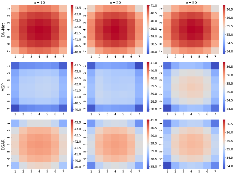
Figure 13: Comparison of the average PSNR for each SAI of denoised LFs produced by various methods. The PSNR values depicted are calculated as the average across the test set derived from the HCI+Inria dataset.

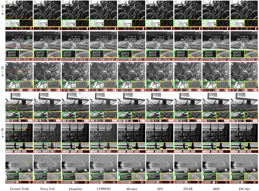
Figure 14: Visual comparisons of denoised LF from different methods over the Stanford Archive dataset. The zoomed selected regions and EPI are shown for better visualization

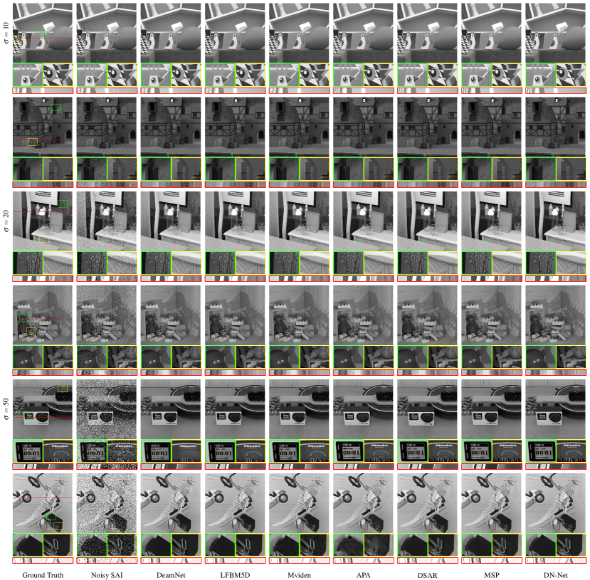
Figure 15: Visual comparisons of denoised LF from different methods over the HCI+Inria dataset. The zoomed selected regions and EPI are shown for better visualization

Figure 16: Visual comparisons of ground-truth depth maps and estimated depth maps from denoised light fields by various methods on the HCI+Inria dataset.

6.3.2 Visual Comparison

Fig. 14 and Fig. 15 present visual comparisons of denoised LFs obtained through different methods across three noise levels $\sigma=10,20$ and $50$. The results indicate that DeamNet, LFBM5D, and Mviden fail to preserve high-frequency details, such as the texture regions of flowers, and generate severe distortions, such as the window frames. Additionally, DeamNet produces hole artifacts in the denoised LFs. While APA yields comparatively better visual results than LFBM5D and DeamNet, it still exhibits blurring artifacts at occlusion boundaries. DSAR and MSP achieve relatively good visual results, but the details in textured regions and occlusion boundaries are not as sharp as those produced by our DN-Net. Visual comparison of the EPIs extracted from the denoised LFs indicates that our method can preserve sharper linear structures, thereby validating its advantage in preserving LF parallax structures during denoising.

Furthermore, we compared the estimated depth maps obtained through different methods using the same depth estimation method Chen et al. (2018b). As shown in Fig. 16, the depth maps generated by our DN-Net are more similar to the ground truth at both smooth regions and occlusion boundaries, indicating that the proposed DN-Net can better preserve the parallax structure than the other methods.

Figure 17: Visual comparisons of different methods on real LF denoising. Our DN-Net trained on Stanford Archive dataset with $\sigma=20$ were selected. The zoomed selected regions and EPI are shown for better visualization

6.3.3 Comparisons on Real LF Denoising

When the lighting of the shooting scene is not sufficient, the light field data will be seriously affected by noise. Therefore, we used the low-light data collected by the Lytro Illum camera and verified the effectiveness of our DN-Net trained on the Stanford Archive dataset and with $\sigma=20$. From the experimental results in Fig. 17, we can observe that our algorithm can effectively remove noise while maintaining clear scene details better.

6.3.4 Comparison of Running Time

We compared the inference time (in seconds) of different methods for LF denoising under HCI+Inria dataset, and Table 6 lists the results. All methods were tested on a desktop with Intel CPU i7-8700 @ 3.70GHz, 32 GB RAM and NVIDIA GeForce RTX 3090. As shown in Table 6, Ours is faster than Alain and Smolic (2017), Tomita et al. (2022), Chen et al. (2018a) and Guo et al. (2022) but slower than Ren et al. (2021) and Wang et al. (2023c).

6.3.5 Ablation Study

We conducted ablation studies on the HCI+Inria dataset with $\sigma=20$ to verify the effectiveness of the extended framework and the impact of the number of stages and feature embedding units.

The number of stages and feature embedding units. We varied the number of iterative stages in the range from 1 to 4 with 6 fixed feature embedding units, and varied the number of feature embedding units, i.e., 4, 6, and 8 with 2 fixed iterative stages. As shown in Table 7, the denoising performance improves with the increase in the number of iterative stages. Moreover, the improvement is more obvious from 1 stage to 3 stages, while slight from 3 stages to 4 stages. What’s more, the performance improves with the number of feature embedding units increasing. To balance the denoising performance and the number of network parameters, we finally choose 2 stages with 6 feature embedding units to process all the LF denoising tasks.

The application of the proposed probabilistic-based feature embedding module to various LF tasks requires a balance between performance and computational efficiency. As a general guideline, we recommend maintaining the number of network parameters within the range of $2M\sim 4M$. This can be achieved using configurations such as $T=3,J=6,C=64$ or $T=6,J=6,C=32$, where $C$ represents the number of feature channels. These initial configurations can be fine-tuned further as per specific requirements.

Table 7: Performance comparisons of our LF denoising method with different numbers of iterative stages and feature embedding units in a probabilistic-based feature embedding module.

		PSNR	SSIM	# Parameters
$T$ = 2	$J$ = 4	40.15	0.959	1.57
	$J$ = 6	40.50	0.962	2.39
	$J$ = 8	40.65	0.963	3.32
$J$ = 6	$T$ = 1	40.01	0.958	1.61
	$T$ = 2	40.50	0.962	2.39
	$T$ = 3	40.72	0.963	3.23
	$T$ = 4	40.76	0.963	4.03

Effectiveness of the proposed noise suppression module and probabilistic-based feature embedding. Our approach combines a noise suppression module with the proposed probabilistic-based feature embedding for LF denoising. To validate the effectiveness of the proposed noise suppression module, we conducted a quantitative comparison of the quality of denoised LF images generated by our method without the noise suppression module (i.e., w/o Noise Suppression).

Furthermore, to evaluate the effectiveness of the proposed probabilistic-based feature embedding, we replaced the probabilistic-based feature embedding $\mathcal{D}(\cdot)$ in each stage with either a stack of 3-D convolution layers or SAS layers while maintaining a similar model size to our framework. The resulting networks were denoted as DN-Conv3D and DN-SAS, respectively, and their performances were compared with the proposed DN-Net in Table 9.

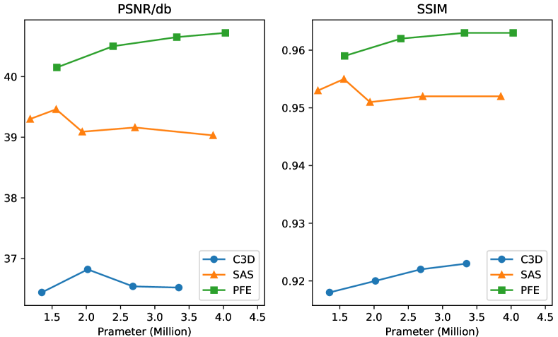
Figure 18: Quantitative results of the proposed denoising framework equipped with different feature embedding extraction methods, i.e., the proposed probabilistic-based feature embedding (PFE), the SAS convolution (SAS), and the 3-D convolution (C3D). The PSNR/SSIM values for the task $\sigma=20$ on the HCI+Inria dataset, as well as the model size, are provided for comparisons.

Table 8: Comparative analysis of the effectiveness of the proposed PFE module on LF spatial and angular super-resolution (SR). We selected $2\times$ spatial SR with $5\times 5$ SAIs and $2\times 2\rightarrow 7\times 7$ angular SR for the comparison. The table presents the PSNR/SSIM results for two tasks, DistgSSR and DistgASR, with and without the integration of PFE.

$2\times$	Model	EPLF	HCInew	HCIold	Inria	STFgtr
Spatial SR	DistgSSR	34.58/0.977	37.76/0.979	44.77/0.995	36.48/0.985	40.29/0.994
	DistgSSR-PFE	34.85/0.978	37.92/0.979	44.86/0.995	36.69/0.986	40.55/0.994
$2\times 2\rightarrow 7\times 7$	Model	HCInew	HCIold	30scenes	Occlusion	Reflective
Angular SR	DistgASR	34.28/0.970	42.12/0.977	43.36/0.995	39.15/0.990	38.85/0.977
	DistgASR-PFE	34.52/0.972	42.33/0.979	43.64/0.995	39.40/0.991	39.08/0.978

Moreover, we proposed a baseline framework without the proposed modules and replaced the feature embedding units with SAS. As shown in Table 9, it can be observed that without the proposed noise suppression module, the value of PSNR decreased by approximately $0.45dB$, thereby validating its effectiveness. Furthermore, the proposed DN-Net outperformed the 3-D convolution, SAS, and template network (DN-Template) in our evaluations, demonstrating the advantage of the proposed probabilistic-based feature embedding. Moreover, the effectiveness of the overall framework was validated by comparing the baseline with the proposed DN-Net, where it can be seen that the value of PSNR improved by $2.3dB$.

To gain further insight into the advantages and disadvantages of commonly used LF feature extraction methods, i.e., the proposed probabilistic-based feature embedding (PFE), SAS convolution (SAS), and 3-D convolution (C3D), we present a performance analysis with parameter quantities in Fig. 18. As demonstrated, the performance of our proposed PFE steadily improves as the number of parameters increases. Whereas the PSNR of SAS and C3D initially improves, but then the performance fluctuates or declines, possibly due to network overfitting. Therefore, our proposed PFE is more suitable for building deeper networks.

Table 9: Effectiveness of the proposed framework in terms of average PSNR and SSIM values.

	PSNR	SSIM	# Parameters
w/o Noise Suppression	40.04	0.959	2.38
Baseline	38.14	0.942	2.46
DN-Conv3D(1)	36.82	0.920	2.02
DN-Conv3D(2)	36.54	0.922	2.68
DN-SAS	38.82	0.950	2.32
DN-Template	40.27	0.960	2.41
DN-Net	40.50	0.962	2.39

6.4 Evaluation on 4-D LF Super-Resolution

In addition to the coded aperture-based compressive LF reconstruction, LF super-resolution approaches, including spatial and angular super-resolution techniques, present an alternative route to achieving high-quality LFs. The spatial-angular trade-offs present in LF cameras have incited the development of several LF super-resolution methods to enhance spatial or angular resolution.

To further validate the efficacy of our Probabilistic-based Feature Embedding (PFE) approach, we conducted experiments based on a recent work Wang et al. (2023a). We specifically applied PFE to two distinct tasks, namely DistgSSR and DistgASR, and retrained the models using the dataset and codes officially released. The results, which provide a performance baseline, are documented in Table 8. To control for potential confounding effects of different network settings (e.g., the use of LeakyReLU), we restructured DistgSSR and DistgASR into template networks and integrated our PFE methodology, yielding DistgSSR-PFE and DistgASR-PFE. In the detailed implementation, PFE is deployed on the Disentangling block of the DistgSSR-PFE network and on both the Disentangling block and Disentangling group of the DistgASR-PFE network. The experimental findings, as outlined in Table 8, clearly demonstrate that our PFE can enhance network performance.

7 Conclusion

We have presented a novel adaptive probabilistic-based feature embedding for LFs. To verify its effectiveness, we evaluated its performance on compressive LF reconstruction and LF denoising, respectively. For compressive LF imaging, we proposed a physically interpretable cycle-consistent framework that incorporates probabilistic-based feature embedding. Our approach can reconstruct 4-D LFs from 2-D measurements with higher quality, improving the PSNR value by approximately 4.5 dB while preserving the LF parallax structure better than state-of-the-art methods. Furthermore, we demonstrate the efficacy of our probabilistic-based feature embedding approach for LF denoising through a carefully designed network. Extensive experiments on diverse datasets demonstrate that our method outperforms state-of-the-art approaches by up to $1.1$ dB.

In future work, the application of our proposed probabilistic-based feature embedding could be potentially broadened to include other tasks within the domain of LF image processing, such as depth estimation. Moreover, our proposed CR-Net exhibits significant potential for direct integration in reconstruction-based LF compression tasks Hou et al. (2018). The inherent capabilities of CR-Net could be leveraged to gather, compress, transmit, and subsequently reconstruct compressed sensing images. This process would yield high-quality light fields, all while necessitating less data.

Data Availability Statements

As indicated in the manuscript, the used datasets are deposited in publicly available repositories.

Conflict of Interest

The authors declare that they do not have any commercial or associative interest that represents a conflict of interest in connection with the work submitted.

References

- Ng et al. [2005] Ren Ng, Marc Levoy, Mathieu Brédif, Gene Duval, Mark Horowitz, and Pat Hanrahan. Light field photography with a hand-held plenoptic camera. PhD thesis, Stanford University, 2005.
- Ng et al. [2006] Ren Ng et al. Digital light field photography, volume 7. stanford university Stanford, 2006.
- Wanner and Goldluecke [2013] Sven Wanner and Bastian Goldluecke. Variational light field analysis for disparity estimation and super-resolution. IEEE Transactions on Pattern Analysis and Machine Intelligence, 36(3):606–619, 2013.
- Wang et al. [2015] Ting-Chun Wang, Alexei A Efros, and Ravi Ramamoorthi. Occlusion-aware depth estimation using light-field cameras. In Proceedings of the IEEE International Conference on Computer Vision (ICCV), pages 3487–3495, 2015.
- Park et al. [2017] In Kyu Park, Kyoung Mu Lee, et al. Robust light field depth estimation using occlusion-noise aware data costs. IEEE Transactions on Pattern Analysis and Machine Intelligence, 40(10):2484–2497, 2017.
- Jin and Hou [2022] Jing Jin and Junhui Hou. Occlusion-aware unsupervised learning of depth from 4-d light fields. IEEE Transactions on Image Processing, 31:2216–2228, 2022.
- Li et al. [2014] Nianyi Li, Jinwei Ye, Yu Ji, Haibin Ling, and Jingyi Yu. Saliency detection on light field. In Proceedings of the IEEE Conference on Computer Vision and Pattern Recognition (CVPR), pages 2806–2813, 2014.
- Wang et al. [2019] Tiantian Wang, Yongri Piao, Xiao Li, Lihe Zhang, and Huchuan Lu. Deep learning for light field saliency detection. In Proceedings of the IEEE/CVF International Conference on Computer Vision (ICCV), pages 8838–8848, 2019.
- Jing et al. [2021] Dong Jing, Shuo Zhang, Runmin Cong, and Youfang Lin. Occlusion-aware bi-directional guided network for light field salient object detection. In Proceedings of the ACM International Conference on Multimedia, pages 1692–1701, 2021.
- Wang et al. [2016] Ting-Chun Wang, Jun-Yan Zhu, Ebi Hiroaki, Manmohan Chandraker, Alexei A Efros, and Ravi Ramamoorthi. A 4d light-field dataset and cnn architectures for material recognition. In European Conference on Computer Vision (ECCV), pages 121–138, 2016.
- Hog et al. [2016] Matthieu Hog, Neus Sabater, and Christine Guillemot. Light field segmentation using a ray-based graph structure. In European Conference on Computer Vision (ECCV), pages 35–50, 2016.
- Inagaki et al. [2018] Yasutaka Inagaki, Yuto Kobayashi, Keita Takahashi, Toshiaki Fujii, and Hajime Nagahara. Learning to capture light fields through a coded aperture camera. In Proceedings of the European Conference on Computer Vision (ECCV), pages 418–434, 2018.
- Vadathya et al. [2020] Anil Kumar Vadathya, Sharath Girish, and Kaushik Mitra. A unified learning-based framework for light field reconstruction from coded projections. IEEE Transactions on Computational Imaging, 6:304–316, 2020.
- Shin et al. [2018] Changha Shin, Hae-Gon Jeon, Youngjin Yoon, In So Kweon, and Seon Joo Kim. Epinet: A fully-convolutional neural network using epipolar geometry for depth from light field images. In Proceedings of the IEEE Conference on Computer Vision and Pattern Recognition (CVPR), pages 4748–4757, 2018.
- Zhang et al. [2019] Shuo Zhang, Youfang Lin, and Hao Sheng. Residual networks for light field image super-resolution. In Proceedings of the IEEE/CVF Conference on Computer Vision and Pattern Recognition (CVPR), pages 11046–11055, 2019.
- Yeung et al. [2019] Henry Wing Fung Yeung, Junhui Hou, Xiaoming Chen, Jie Chen, Zhibo Chen, and Yuk Ying Chung. Light field spatial super-resolution using deep efficient spatial-angular separable convolution. IEEE Transactions on Image Processing, 28(5):2319–2330, 2019.
- Wu et al. [2017] Gaochang Wu, Mandan Zhao, Liangyong Wang, Qionghai Dai, Tianyou Chai, and Yebin Liu. Light field reconstruction using deep convolutional network on epi. In Proceedings of the IEEE Conference on Computer Vision and Pattern Recognition (CVPR), pages 6319–6327, 2017.
- Wu et al. [2019] Gaochang Wu, Yebin Liu, Qionghai Dai, and Tianyou Chai. Learning sheared epi structure for light field reconstruction. IEEE Transactions on Image Processing, 28(7):3261–3273, 2019.
- Heber et al. [2017] Stefan Heber, Wei Yu, and Thomas Pock. Neural epi-volume networks for shape from light field. In Proceedings of the IEEE International Conference on Computer Vision (ICCV), pages 2252–2260, 2017.
- Yeung et al. [2018] Henry Wing Fung Yeung, Junhui Hou, Jie Chen, Yuk Ying Chung, and Xiaoming Chen. Fast light field reconstruction with deep coarse-to-fine modeling of spatial-angular clues. In European Conference on Computer Vision (ECCV), pages 137–152, 2018.
- Jin et al. [2020a] Jing Jin, Junhui Hou, Jie Chen, and Sam Kwong. Light field spatial super-resolution via deep combinatorial geometry embedding and structural consistency regularization. In Proceedings of the IEEE/CVF Conference on Computer Vision and Pattern Recognition (CVPR), pages 2260–2269, June 2020a.
- Guo et al. [2020] Mantang Guo, Junhui Hou, Jing Jin, Jie Chen, and Lap-Pui Chau. Deep spatial-angular regularization for compressive light field reconstruction over coded apertures. In Proceedings of the European Conference on Computer Vision (ECCV), pages 278–294, 2020.
- Jin et al. [2022] Jing Jin, Junhui Hou, Jie Chen, Huanqiang Zeng, Sam Kwong, and Jingyi Yu. Deep coarse-to-fine dense light field reconstruction with flexible sampling and geometry-aware fusion. IEEE Transactions on Pattern Analysis and Machine Intelligence, 44(4):1819–1836, 2022.
- Wang et al. [2020] Yingqian Wang, Longguang Wang, Jungang Yang, Wei An, Jingyi Yu, and Yulan Guo. Spatial-angular interaction for light field image super-resolution. In European Conference on Computer Vision (ECCV), pages 290–308, 2020.
- Wang et al. [2021a] Yingqian Wang, Jungang Yang, Longguang Wang, Xinyi Ying, Tianhao Wu, Wei An, and Yulan Guo. Light field image super-resolution using deformable convolution. IEEE Transactions on Image Processing, 30:1057–1071, 2021a.
- Wang et al. [2023a] Yingqian Wang, Longguang Wang, Gaochang Wu, Jungang Yang, Wei An, Jingyi Yu, and Yulan Guo. Disentangling light fields for super-resolution and disparity estimation. IEEE Transactions on Pattern Analysis and Machine Intelligence, 45(1):425–443, 2023a.
- Wang et al. [2022] Shunzhou Wang, Tianfei Zhou, Yao Lu, and Huijun Di. Detail-preserving transformer for light field image super-resolution. In Proceedings of the AAAI Conference on Artificial Intelligence, volume 36, pages 2522–2530, 2022.
- Liang et al. [2022] Zhengyu Liang, Yingqian Wang, Longguang Wang, Jungang Yang, and Shilin Zhou. Light field image super-resolution with transformers. IEEE Signal Processing Letters, 29:563–567, 2022.
- Liang et al. [2023] Zhengyu Liang, Yingqian Wang, Longguang Wang, Jungang Yang, Shilin Zhou, and Yulan Guo. Learning non-local spatial-angular correlation for light field image super-resolution. In Proceedings of the IEEE International Conference on Computer Vision (ICCV), 2023.
- Wilburn et al. [2005] Bennett Wilburn, Neel Joshi, Vaibhav Vaish, Eino-Ville Talvala, Emilio Antunez, Adam Barth, Andrew Adams, Mark Horowitz, and Marc Levoy. High performance imaging using large camera arrays. ACM Trans. Graph., 24(3):765––776, 2005.
- [31] Vaish Vaibhav and Adams Andrew. Light field gantry. https://raytrix.de/.
- Lytro [2016] Lytro. http://lightfield.stanford.edu/acq.html, 2016.
- [33] RayTrix. 3d light field camera technology. https://raytrix.de/.
- Van Duong et al. [2023] Vinh Van Duong, Thuc Nguyen Huu, Jonghoon Yim, and Byeungwoo Jeon. Light field image super-resolution network via joint spatial-angular and epipolar information. IEEE Transactions on Computational Imaging, 9:350–366, 2023.
- Wang et al. [2023b] Yingqian Wang, Longguang Wang, Zhengyu Liang, Jungang Yang, and et al. Ntire 2023 challenge on light field image super-resolution: Dataset, methods and results. In IEEE/CVF Conference on Computer Vision and Pattern Recognition Workshops (CVPRW), pages 1320–1335, 2023b.
- Chen et al. [2022] Yangling Chen, Shuo Zhang, Song Chang, and Youfang Lin. Light field reconstruction using efficient pseudo 4d epipolar-aware structure. IEEE Transactions on Computational Imaging, 8:397–410, 2022.
- Yang et al. [2023] Jiangxin Yang, Lingyu Wang, Lifei Ren, Yanpeng Cao, and Yanlong Cao. Light field angular super-resolution based on structure and scene information. Applied Intelligence, 53(4):4767–4783, 2023.
- Wang et al. [2017] Yuwang Wang, Yebin Liu, Wolfgang Heidrich, and Qionghai Dai. The light field attachment: Turning a dslr into a light field camera using a low budget camera ring. IEEE Transactions on Visualization and Computer Graphics, 23(10):2357–2364, 2017.
- Jin et al. [2023] Jing Jin, Mantang Guo, Junhui Hou, Hui Liu, and Hongkai Xiong. Light field reconstruction via deep adaptive fusion of hybrid lenses. IEEE Transactions on Pattern Analysis and Machine Intelligence, 45(10):12050–12067, 2023.
- Guo et al. [2022] Mantang Guo, Junhui Hou, Jing Jin, Jie Chen, and Lap-Pui Chau. Deep spatial-angular regularization for light field imaging, denoising, and super-resolution. IEEE Transactions on Pattern Analysis and Machine Intelligence, 44(10):6094–6110, 2022.
- Babacan et al. [2012] S Derin Babacan, Reto Ansorge, Martin Luessi, Pablo Ruiz Matarán, Rafael Molina, and Aggelos K Katsaggelos. Compressive light field sensing. IEEE Transactions on Image Processing, 21(12):4746–4757, 2012.
- Marwah et al. [2013] Kshitij Marwah, Gordon Wetzstein, Yosuke Bando, and Ramesh Raskar. Compressive light field photography using overcomplete dictionaries and optimized projections. ACM Transactions on Graphics., 32(4):1–12, 2013.
- Lamba et al. [2020] Mohit Lamba, Kranthi Kumar Rachavarapu, and Kaushik Mitra. Harnessing multi-view perspective of light fields for low-light imaging. IEEE Transactions on Image Processing, 30:1501–1513, 2020.
- Zhang et al. [2017] Kai Zhang, Wangmeng Zuo, Yunjin Chen, Deyu Meng, and Lei Zhang. Beyond a gaussian denoiser: Residual learning of deep cnn for image denoising. IEEE Transactions on Image Processing, 26(7):3142–3155, 2017.
- Tassano et al. [2020] Matias Tassano, Julie Delon, and Thomas Veit. Fastdvdnet: Towards real-time deep video denoising without flow estimation. In Proceedings of the IEEE Conference on Computer Vision and Pattern Recognition (CVPR), pages 1354–1363, 2020.
- Yoon et al. [2015] Youngjin Yoon, Hae-Gon Jeon, Donggeun Yoo, Joon-Young Lee, and In So Kweon. Learning a deep convolutional network for light-field image super-resolution. In Proceedings of the IEEE International Conference on Computer Vision (ICCV) workshops, pages 24–32, 2015.
- Wang et al. [2018] Yunlong Wang, Fei Liu, Zilei Wang, Guangqi Hou, Zhenan Sun, and Tieniu Tan. End-to-end view synthesis for light field imaging with pseudo 4dcnn. In European Conference on Computer Vision (ECCV), pages 333–348, 2018.
- Jin et al. [2020b] Jing Jin, Junhui Hou, Hui Yuan, and Sam Kwong. Learning light field angular super-resolution via a geometry-aware network. In Proceedings of the AAAI conference on artificial intelligence, volume 34, pages 11141–11148, 2020b.
- Gupta et al. [2017] Mayank Gupta, Arjun Jauhari, Kuldeep Kulkarni, Suren Jayasuriya, Alyosha Molnar, and Pavan Turaga. Compressive light field reconstructions using deep learning. In Proceedings of the IEEE Conference on Computer Vision and Pattern Recognition Workshops (CVPRW), pages 11–20, 2017.
- Chen et al. [2018a] Jie Chen, Junhui Hou, and Lap-Pui Chau. Light field denoising via anisotropic parallax analysis in a cnn framework. IEEE Signal Processing Letters, 25(9):1403–1407, 2018a.
- Wang et al. [2023c] Xianglang Wang, Youfang Lin, and Shuo Zhang. Multi-stream progressive restoration for low-light light field enhancement and denoising. IEEE Transactions on Computational Imaging, 9:70–82, 2023c.
- Lyu et al. [2021] Xianqiang Lyu, Zhiyu Zhu, Mantang Guo, Jing Jin, Junhui Hou, and Huanqiang Zeng. Learning spatial-angular fusion for compressive light field imaging in a cycle-consistent framework. In Proceedings of the ACM International Conference on Multimedia, pages 4613–4621, 2021.
- Liang et al. [2008] Chia-Kai Liang, Tai-Hsu Lin, Bing-Yi Wong, Chi Liu, and Homer H Chen. Programmable aperture photography: multiplexed light field acquisition. In ACM SIGGRAPH 2008 papers, pages 1–10. 2008.
- Ashok and Neifeld [2010] Amit Ashok and Mark A Neifeld. Compressive light field imaging. In Three-Dimensional Imaging, Visualization, and Display 2010 and Display Technologies and Applications for Defense, Security, and Avionics IV, volume 7690, pages 221–232, 2010.
- Alain and Smolic [2017] Martin Alain and Aljosa Smolic. Light field denoising by sparse 5d transform domain collaborative filtering. In International Workshop on Multimedia Signal Processing (MMSP), pages 1–6. IEEE, 2017.
- Dabov et al. [2007] Kostadin Dabov, Alessandro Foi, Vladimir Katkovnik, and Karen Egiazarian. Image denoising by sparse 3-d transform-domain collaborative filtering. IEEE Transactions on Image Processing, 16(8):2080–2095, 2007.
- Li et al. [2013] Zeyu Li, Harlyn Baker, and Ruzena Bajcsy. Joint image denoising using light-field data. In IEEE International Conference on Multimedia and Expo Workshops (ICMEW), pages 1–6. IEEE, 2013.
- Beck and Teboulle [2009] Amir Beck and Marc Teboulle. Fast gradient-based algorithms for constrained total variation image denoising and deblurring problems. IEEE Transactions on Image Processing, 18(11):2419–2434, 2009.
- Sepas-Moghaddam et al. [2016] Alireza Sepas-Moghaddam, Paulo Lobato Correia, and Fernando Pereira. Light field denoising: exploiting the redundancy of an epipolar sequence representation. In 3DTV-Conference: The True Vision-Capture, Transmission and Display of 3D Video (3DTV-CON), pages 1–4. IEEE, 2016.
- Maggioni et al. [2012] Matteo Maggioni, Giacomo Boracchi, Alessandro Foi, and Karen Egiazarian. Video denoising, deblocking, and enhancement through separable 4-d nonlocal spatiotemporal transforms. IEEE Transactions on Image Processing, 21(9):3952–3966, 2012.
- Dansereau et al. [2013] Donald G Dansereau, Daniel L Bongiorno, Oscar Pizarro, and Stefan B Williams. Light field image denoising using a linear 4d frequency-hyperfan all-in-focus filter. In Computational Imaging XI, volume 8657, pages 176–189. SPIE, 2013.
- Premaratne et al. [2020] Sanduni U Premaratne, Namalka Liyanage, Chamira US Edussooriya, and Chamith Wijenayake. Real-time light field denoising using a novel linear 4-d hyperfan filter. IEEE Transactions on Circuits and Systems I: Regular Papers, 67(8):2693–2706, 2020.
- Tomita et al. [2022] Keigo Tomita, Chihiro Tsutake, Keita Takahashi, and Toshiaki Fujii. Denoising multi-view images by soft thresholding: A short-time dft approach. Signal Processing: Image Communication, 105:116710, 2022.
- Liu et al. [2019] Hanxiao Liu, Karen Simonyan, and Yiming Yang. Darts: Differentiable architecture search. In International Conference on Learning Representations (ICLR), 2019.
- Wang et al. [2021b] Naiyan Wang, Shiming XIANG, Chunhong Pan, et al. You only search once: Single shot neural architecture search via direct sparse optimization. IEEE Transactions on Pattern Analysis and Machine Intelligence, 43(9):2891–2904, 2021b.
- Gal and Ghahramani [2016] Yarin Gal and Zoubin Ghahramani. Dropout as a bayesian approximation: Representing model uncertainty in deep learning. In International Conference on Machine Learning, pages 1050–1059. PMLR, 2016.
- Damianou and Lawrence [2013] Andreas Damianou and Neil D Lawrence. Deep gaussian processes. In Artificial intelligence and statistics, pages 207–215. PMLR, 2013.
- Jang et al. [2017] Eric Jang, Shixiang Gu, and Ben Poole. Categorical reparameterization with gumbel-softmax. In International Conference on Learning Representations (ICLR), 2017.
- Kalantari et al. [2016] Nima Khademi Kalantari, Ting-Chun Wang, and Ravi Ramamoorthi. Learning-based view synthesis for light field cameras. ACM Transactions on Graphics., 35(6):1–10, 2016.
- Honauer et al. [2016] Katrin Honauer, Ole Johannsen, Daniel Kondermann, and Bastian Goldluecke. A dataset and evaluation methodology for depth estimation on 4d light fields. In Asian Conference on Computer Vision (ACCV), pages 19–34, 2016.
- Shi et al. [2019] Jinglei Shi, Xiaoran Jiang, and Christine Guillemot. A framework for learning depth from a flexible subset of dense and sparse light field views. IEEE Transactions on Image Processing, 28(12):5867–5880, 2019.
- Kingma and Ba [2014] Diederik P Kingma and Jimmy Ba. Adam: A method for stochastic optimization. arXiv preprint arXiv:1412.6980, 2014.
- Smith and Topin [2019] Leslie N Smith and Nicholay Topin. Super-convergence: Very fast training of neural networks using large learning rates. In Artificial Intelligence and Machine Learning for Multi-Domain Operations Applications, volume 11006, pages 369–386, 2019.
- Chen et al. [2018b] Jie Chen, Junhui Hou, Yun Ni, and Lap-Pui Chau. Accurate light field depth estimation with superpixel regularization over partially occluded regions. IEEE Transactions on Image Processing, 27(10):4889–4900, 2018b.
- Ren et al. [2021] Chao Ren, Xiaohai He, Chuncheng Wang, and Zhibo Zhao. Adaptive consistency prior based deep network for image denoising. In Proceedings of the IEEE Conference on Computer Vision and Pattern Recognition (CVPR), pages 8596–8606, 2021.
- [76] Abhilash Sunder Raj, Michael Lowney, and Gordon Wetzstein. Stanford lytro light field archive. http://lightfields.stanford.edu/LF2016.html.
- Hou et al. [2018] Junhui Hou, Jie Chen, and Lap-Pui Chau. Light field image compression based on bi-level view compensation with rate-distortion optimization. IEEE Transactions on Circuits and Systems for Video Technology, 29(2):517–530, 2018.