Energy Management for a DM-i Plug-in Hybrid Electric Vehicle via Continuous-Discrete Reinforcement Learning

Abstract

Energy management strategy (EMS) is a key technology for plug-in hybrid electric vehicles (PHEVs). The energy management of PHEVs needs to output continuous variables such as engine torque, as well as discrete variables such as clutch engagement or disengagement. This type of problem is a mixed-integer programming problem. In addition, the hybrid powertrain system is highly nonlinear and complex. Designing an efficient EMS is a challenging task. We establish a control-oriented mathematical model for a BYD DM-i hybrid powertrain system from the perspective of mixed-integer programming. Then, an EMS based on continuous-discrete reinforcement learning is introduced, which can output both continuous and discrete variables simultaneously. Finally, the effectiveness of the proposed control strategy is verified by comparing EMS based on charge-depleting charge-sustaining (CD-CS) and Dynamic Programming (DP). The simulation results show that the reinforcement learning EMS can improve energy efficiency by 10.08% compared to the CD-CS EMS, and the fuel economy gap is about 6.4% compared with the benchmark global optimum based on DP.

I Introduction

Energy conservation and reducing consumption are effective ways to achieve low-carbon development of automotive technology. Plug-in hybrid electric vehicles (PHEVs) combine the advantages of electric vehicles and traditional gasoline vehicles, which can save energy and reduce emissions while avoiding the range anxiety associated with pure electric vehicles. They play a significant role in the current commercialization of new energy vehicles. The study of EMS in PHEVs involves the coordination between electric energy and fuel, which is the crucial technology that impacts the fuel economy and emissions of the vehicle [1]. Therefore, a reasonable and effective EMS is crucial for improving the overall performance of PHEVs and can also contribute to achieving sustainable development goals of the automotive manufacturing industry.

I-A Literature Review

In order to improve the fuel economy of PHEVs, a significant amount of research has been conducted over the past few decades on energy management control strategies for PHEVs. EMS can be divided into rule-based, optimization-based, and learning-based methods[2]. Rule-based strategies select the operating mode based on pre-defined rules and can be further divided into deterministic rule-based strategies[3] and fuzzy logic-based strategies[4]. Rule-based EMS is widely used due to their simplicity and practicality, but they cannot obtain the globally optimal solution[5]. In order to further enhance the control performance of rule-based strategies, some studies have utilized algorithms for rule optimization. In [6], particle swarm optimization algorithm is used to optimize the parameters of fuzzy rules, which improves the fuel economy of vehicles. In [7], the mode switching threshold was optimized using simulated annealing and particle swarm optimization algorithms, resulting in an ideal mode switching sequence.

In optimization-based control strategies, the PHEV’s EMS is typically abstracted as a constrained nonlinear optimization problem. Optimization-based control strategies can be divided into two categories: global optimization and real-time optimization[8]. Global optimization mainly includes DP[9] and Pontryagin’s minimum principle (PMP)[10]. The DP algorithm aims to optimize the fuel economy of the entire vehicle by establishing a global optimization mathematical model with constraints. Based on the Bellman optimality principle, the algorithm solves for the optimal energy allocation between the engine and battery by using state transition equations. If the entire driving cycle information is obtained in advance, the global optimal EMS can be obtained through DP algorithm [11]. Although DP-based strategies are effective in obtaining the globally optimal fuel economy of PHEVs, driving cycle information is usually unknown in practical applications, so DP is not suitable for real-time control. It is usually used as a benchmark for fuel economy. The EMS based on PMP algorithm is to obtain the optimal control strategy by minimizing the Hamilton equation in real time [12]. In [13], the PMP is used to optimize the EMS of a hybrid energy storage system. The simulation results show that in the energy management of power-split HEVs, the difference between the PMP-based control strategy and the DP strategy is less than 1% , which proves the flexibility and effectiveness of the strategy. Compared with the DP algorithm, the PMP calculation is relatively small. However, it is difficult to solve the EMS directly through PMP due to the influence of state constraints and the complexity of the system model. Moreover, PMP also requires a known driving cycle,which is not available in real-world driving.

Model predictive control (MPC) [14] and the minimum equivalent fuel consumption strategy (ECMS) [15] are typical real-time optimization algorithms. MPC is based on rolling optimization, which transforms the optimization process into a finite predictive range, reducing computational complexity and having the potential for real-time control. However, model accuracy and prediction horizon length will affect fuel economy [16]. The core idea of ECMS is to use equivalent coefficients to convert the power consumption of the motor into fuel consumption, and to solve the optimal energy allocation problem of PHEVs with the minimum equivalent fuel consumption as the objective function [17]. However, ECMS results are very sensitive to equivalent coefficients, which are affected by driving conditions, battery SOC, driving style, road gradient, and other factors, which affect the calculation accuracy of EMS.

Reinforcement learning (RL) has been applied to energy management in PHEVs, and the results have been promising. In [18], a Q-learning based EMS for PHEVs was proposed, which makes decisions on the current system state by looking up Q-table. It does not need to rely on prior knowledge of future driving conditions to make optimal decisions. Simulation results show that the fuel economy of the proposed EMS is improved by 11.93% compared with the binary mode control strategy. In [19], a HEV EMS based on SARSA algorithm was studied. Unlike Q-learning, SARSA is on-policy. During the interaction between agent and environment, more searches can be conducted, which is conducive to the accuracy of agent learning. The simulation results revealed that compared with Q-learning, SARSA algorithm could achieve better performance.

Although RL-based EMS has some significant advantages, traditional RL require the discretization of state and action spaces. As the dimensions of the state and action spaces increase, it will lead to ”curse of dimensionality”. Furthermore, traditional RL stores data in tables, which requires lots of time and computational resources to complete learning. To improve the performance of RL, some researchers have combined deep learning (DL) with RL and proposed an online EMS called Deep Reinforcement Learning (DRL) [20]. The emergence of DRL algorithm solves the problem of the traditional RL algorithm’s tendency to fall into the dimensionality catastrophe due to discretization. Currently, the mainstream of DRL is discrete reinforcement learning and continuous reinforcement learning [21, 22]. In the case of continuous problems, the action space of discrete reinforcement learning is limited, so it is necessary to discretize continuous actions. In [23], a power split hybrid electric bus EMS based on DQL was proposed. Compared with the RL-based strategy, the optimality and adaptability of the DQL-based strategy under different driving conditions were verified. Compared with the Q-learning strategy with the same model, the DQL strategy performs better in terms of training difficulty and the influence of different state variables on the Q function. To solve the problem of overestimation, EMS based on dual deep Q learning (DDQL) was applied to hybrid tracked vehicles in [24]. The simulation results show that the fuel economy is improved by 7.1% compared to the DQL algorithm.

Although discrete reinforcement learning performs well, it inevitably introduces discretization errors when discretizing action variables and cannot obtain an accurate solution. To solve the problem of discrete control variables, an EMS based on Deep Deterministic Policy Gradient (DDPG) was proposed in [25]. DDPG avoids the discretization of the action space and can output continuous control variables. Simulation results show that compared with the DQN algorithm, the DDPG algorithm converges faster and is more robust. To solve the problem that DDPG’s high action value estimation may lead to unstable training, an EMS based on TD3 was employed in [26]. Simulation results show that under stable and transient driving cycles, the EMS based on TD3 algorithm has better fuel economy.

In practical energy management systems, there are often both continuous control variables such as the output torque of the engine and motor and discrete control variables such as the switch of the clutch and the gear of the transmission.The above methods cannot directly obtain both continuous and discrete control inputs, witch is difficult to apply to real-time driving conditions. Currently, few articles have applied continuous-discrete reinforcement learning to the energy management of HEVs. In [27], continuous-discrete reinforcement learning was used to optimize the energy management of a hybrid electric bus with a continuously variable transmission, and the best energy management of the hybrid bus was solved based on DDPG. In [28], the Coach-Actor-Double Critic reinforcement learning framework was used for the energy management of a hybrid electric bus. The article further considers the switching status of the engine and uses continuous reinforcement learning to output the engine status. When the output value is less than 0.5, the engine is turned off, otherwise, it is turned on. In [29], continuous-discrete reinforcement learning was used to optimize the energy management of a HEV with a 5-speed automatic transmission. The article uses DDPG to control the engine switch and DQN to control the gear position of the transmission, outputting continuous and discrete variables separately, but without combining Actor-Critic learning and Q-learning. The above articles demonstrate that compared to traditional optimization methods, continuous-discrete reinforcement learning can achieve near-optimal control.

I-B Motivation and innovation

The BYD DMi hybrid electric vehicles are very popular in China, but there is currently a lack of literature specifically focused on the DM-i hybrid system. Additionally, to the author’s knowledge, while continuous-discrete RL has achieved some success in the energy management of non-plug-in hybrid vehicles, there is no literature that applies continuous-discrete RL to the energy management of series-parallel PHEVs. Based on these research gaps, this article takes the BYD DM-i PHEV as the research object, establishes a vehicle powertrain model, and applies state-of-the-art continuous-discrete RL to solve energy management, achieving approximate optimal control of the energy management of the DM-i PHEV.

The main contributions of this paper are summarized as follows:

(1) Modeling the BYD DM-i hybrid system from the perspective of mixed integer programming.

(2) A rule-based EMS is proposed to realize the torque distribution of the engine and motor, by analyzing the working mode of the DM-i hybrid system.

(3) Applying a state-of-the-art continuous-discrete reinforcement learning algorithm for the optimal energy management of the DM-i hybrid system, achieving simultaneous selection of continuous and discrete actions.

I-C Organization

The rest of this paper is organized as follows: Section 2 models the BYD DM-i PHEV. Section 3 introduces the continuous-discrete reinforcement learning PDQN-TD3 algorithm. Section 4 describes the EMS based on the PDQN-TD3 algorithm, and compares the EMS based on PDQN-TD3 with those based on CD-CS and DP approaches. Section 5 concludes the paper.

II DM-i Hybrid Power System Modeling

Modeling of hybrid systems is the foundation for designing EMSs. In this section, we consider the BYD DM-i PHEV system as shown in Fig. 1, which consists of components such as an engine, a clutch, a generator, a drive motor, and a power battery. The key component parameters are shown in Table I. In this type of hybrid system, both the engine and battery serve as energy sources for the powertrain. The engine and drive motor serve as the power sources for the vehicle. By controlling the clutch, engine, and motor state, it is possible to realize five operation modes: EV mode, series mode, parallel mode, engine driving mode, and energy recovery mode.

Figure 1: Configuration of the BYD DM-i PHEV.

TABLE I: Main Parameters of the PHEV

Component	Parameter	Unit	Value
	Mass	kg	1500
	Windward area	m2	2.36
	Air drag coefficient	-	0.28
Vehicle	Tyre radius	m	0.3382
	Rolling resistance coefficient	-	0.012
	EV mode transmission ratio	-	10.126
	Parallel mode transmission ratio	-	2.8
	Series mode transmission ratio	-	2.07
	Maximum angular velocity	rpm	6000
Engine	Maximum power	kW	81
	Maximum torque	Nm	120
	Maximum angular velocity	rpm	16000
Motor	Maximum power	kW	132
	Maximum torque	Nm	325
Generator	Maximum angular velocity	rpm	13000
	Maximum power	kW	55
Battery	Voltage	kV	3.2
	Capacity	Ah	26

II-A Vehicle Dynamics

For hybrid powertrain systems, the powertrain must obey the torque balance equation:

$$T_{d} =T_{e}i_{e}i_{c}\eta_{t}+T_{m}i_{m}\eta_{m}\eta_{t}+T_{b}$$ (1)

where $T_{d}$ denotes the required driving torque of PHEV; $T_{e}$ is engine torque; $i_{e}$ is engine transmission ratio; $i_{c}$ denotes clutch engagement/disengagement, with a value of either 1 or 0; $T_{m}$ is motor torque; $i_{m}$ is motor transmission ratio; $T_{b}$ is break torque; $\eta_{t}$ and $\eta_{m}$ are the mechanical and motor efficiencies, respectively.

According to the longitudinal dynamics equation of the vehicle, the required torque of the powertrain system is established as:

$$T_{d} =[ma+0.5C_{d}\rho Av^{2}+\mu mgcos(\theta)+mgsin(\theta)]r$$ (2)

$$w_{d} =\frac{v}{r}$$ (3)

where $m$ is curb weight; $a$ represents vehicle acceleration; $C_{d}$ is air drag coefficient; $\rho$ is air density; $A$ is the windward area, $v$ is the longitudinal vehicle velocity without regard to wind speed, $\mu$ is rolling coefficient of road; $g$ is the gravity acceleration; $\theta$ is the road slope; $r$ is the wheel radius; $\omega_{d}$ is the wheel speed.

II-B Engine Model

The fuel economy of engine is a key factor to evaluate the EMS of hybrid system. In this article, experimental modeling method is used for engine modeling. Given the engine speed and torque, the instantaneous fuel consumption rate can be obtained by interpolating the engine fuel consumption map as shown in Fig.2. The engine fuel consumption per unit time is given by Eq. (4):

$$\dot{m}_{f}=P_{e}b_{e}=T_{e}\omega_{e}b_{e}$$ (4)

where $P_{e}$ is engine power, $b_{e}$ is the effective fuel consumption of engine according to BSFC in Fig.2, $\omega_{e}$ is engine angular velocity.

In the DM-i hybrid system, the controller controls the connection and disconnection between the engine and the wheels by controlling the engagement/disengagement of the clutch. When the clutch is disconnected, the engine and wheels are decoupled, the engine speed is independent of vehicle speed, and the engine operates in the optimal working curve. When the clutch is closed, the engine speed and the wheels speed are coupled to each other, and the engine speed adjusts according to the vehicle’s speed.Therefore the engine speed can be expressed by the following equation:

$$\omega_{e}=\omega_{d}i_{e}i_{c}+f(T_{e})(1-i_{c})$$ (5)

where $f(T_{e})$ represents the look-up table between engine speed and torque when the engine operates along the optimal economic working curve.

Figure 2: Engine fuel consumption map, where the unit of BSFC is g/kW·h.

II-C Drive Motor and Generator Models

The DM-i hybrid system has two electric motors, namely the drive motor and the generator. The drive motor provides torque output during driving and is responsible for energy recovery during braking. The generator mainly serves as an auxiliary unit, converting mechanical energy into electrical energy, ensuring the engine’s quick start, and adjusting the engine speed to make it work in the economic range. The motor’s map is shown in Fig. 3.

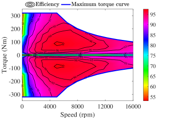
Figure 3: Efficiency map of the driving motor.

For the drive motor, the motor speed and motor torque are written as:

$$\omega_{m}=\omega_{d}i_{m}$$ (6)

$$T_{m}=(T_{d}-T_{b}-T_{e}i_{e}i_{c}\eta_{t})/{i_{m}\eta_{m}\eta_{t}}$$ (7)

where $\omega_{m}$ is the driving motor speed.

To reduce the computational overhead of the RL and DP algorithm, we optimized Eq.(7) by merging $T_{m}$ and $T_{b}$ into $T_{mb}$, thus eliminating the need to control $T_{b}$.

$$\begin{split}T_{mb}=T_{m}i_{m}\eta_{m}\eta_{t}+T_{b}=T_{d}-T_{e}i_{e}i_{c}\eta_{t}\end{split}$$ (8)

The $T_{m}$ and $T_{b}$ can be obtained by Eq.(7):

$$\ \ T_{m}=\begin{cases}{-f(\omega_{m})},\qquad&{\rm if}\;T_{mb}\textless-f(\omega_{m})\\ {T_{mb}/i_{m}\eta_{m}\eta_{t}},\qquad&\rm{else}\end{cases}$$ (9)

$$\ \ T_{b}=\begin{cases}{T_{mb}-T_{m}i_{m}\eta_{m}\eta_{t}=T_{mb}+f(\omega_{m})i_{m}\eta_{m}\eta_{t}},\\ \qquad\qquad\qquad\qquad\qquad\qquad\qquad{\rm if}\;T_{mb}\textless-f(\omega_{m})\\ {0},\qquad\qquad\qquad\qquad\qquad\qquad\;\;\;\;\rm{else}\end{cases}$$ (10)

where $f(\omega_{m})$ represents the maximum torque of the motor at the current speed.

For Eq. (9) and (10), when $T_{mb}$ is less than the motor’s energy recovery upper limit ($T_{mb}<-f(\omega_{m})$), the vehicle enters a braking state. The motor recovers energy at its maximum capacity, while the mechanical brake ($T_{b}$) provides the remaining braking force. When $T_{mb}>-f(\omega_{m})$, the motor assumes the role of energy recovery if $T_{mb}<0$, and driving if $T_{mb}>0$. In both scenarios, the utilization of a mechanical brake ($T_{b}$) is unnecessary.

For the generator, the speed and torque are written as:

$$\omega_{g}=\omega_{e}/i_{g}$$ (11)

$$T_{g}=T_{e}i_{g}\eta_{g}(1-i_{c})$$ (12)

where $\omega_{g}$ is the generator speed; $T_{g}$ is the generator torque; $\eta_{g}$ is the generator efficiency.

II-D Battery Model

The power battery is used to provide the electric energy required by the motor during driving, and can also store the energy recovered by the motor during braking. This paper does not consider the effect of temperature on the internal characteristics of the battery and establishes the dynamic equation of the battery state of charge (SOC) based on the internal resistance of the battery, as shown in the following equations:

$$P_{b}=P_{m}+P_{g}+P_{aux}$$ (13)

$$P_{b}=V_{oc}I_{b}-R_{b}I^{2}_{b}$$ (14)

$$\dot{SOC}=-\frac{V_{oc}-\sqrt{V^{2}_{oc}-4R_{b}P_{b}}}{2R_{b}Q_{b}}$$ (15)

where $P_{b}$ is battery power; $P_{aux}$ is the auxiliary power consumption of the vehicle; $V_{oc}$ is the open circuit voltage; $I_{b}$ is battery current; $R_{b}$ is battery resistance. Ignoring the effects of battery aging and temperature, the relationship between $SOC$, battery internal resistance, and open circuit voltage is shown in Fig.4.

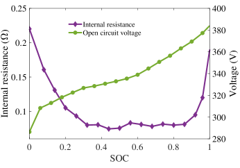
Figure 4: Open-circuit voltage and internal resistance of battery.

III PDQN-TD3 Continuous-Discrete Reinforcement Learning Algorithm

Currently, RL methods mostly focus on either continuous action spaces or discrete action spaces, but many engineering control problems involve both continuous and discrete variables, which is referred to as mixed action space. For example, during the driving process of PHEVs, the torque of the engine is a continuous variable, while the clutch switch is a discrete variable. In mixed action space, the agent needs to make simultaneous discrete and continuous choices. In this section, based on the Actor-Critic framework, the PDQN-TD3 algorithm is proposed to deal with the mixed action space problem.

III-A Principles of Reinforcement Learning

RL is a trial-and-error based learning method. In RL, an agent learns how to make optimal decisions by interacting with its environment. The interaction process between agent and environment can be described using Markov decision processes (MDP). In a MDP, the agent is in a state, can choose an action, then receives a reward signal from the environment and transitions to a new state. The MDP model describes the relationship between state, action, reward and transition probability in this process. RL formulates the optimal strategy by learning the MDP model, which includes learning the relationships between state, action, reward, and transition probabilities. The MDP can be represented as:

$$P_{ss^{\prime}}^{a} =P[s_{t+1}=s^{\prime}|s_{t}=s,a_{t}=a]$$ (16)

where $s_{t}$ represents the state at time $t$, $a_{t}$ represents the action taken at time $t$, $P_{ss^{\prime}}^{a}$ represents the probability of state transition, $s$ represents the current state, $s^{\prime}$ represents the next state, $a$ represents the current action, $P$ is a probability function.

In the state transition process of Eq. (16), a reward $R$ is generated. Given a policy $\pi$, the cumulative reward $G$ obtained by agent in the interaction process is:

$$G_{t} =R_{t+1}+\gamma R_{t+2}+...+\gamma^{t+k}R_{t+1+k}=\sum_{k=0}^{\infty}\gamma^{k}R_{t+1+k}$$ (17)

where $\gamma\in[0,1]$ is the reward discount factor; $R_{t+1}$ represents the immediate reward at time $t+1$.

The ultimate goal of the agent is to find the optimal strategy $\pi^{*}$ to maximize the cumulative reward.

$$\pi^{*}{(s,a)} =\mathop{\rm argmax}\limits_{a}\ E[G_{t}]$$ (18)

where $\pi^{*}(s,a)$ represents the optimal policy and $E$ represents the expectation.

To obtain the optimal strategy, use Q-values to evaluate the superiority or inferiority of the policy $\pi$:

$$Q_{\pi}(s,a) =E[R_{t}+\gamma R_{t+1}+\gamma^{2}R_{t+2}+...|s_{t}=s,a_{t}=a)]$$ (19)

Simplified further, the formula can be expressed as follows:

$$Q_{\pi}(s,a) =E[R_{t}+\gamma Q(s^{\prime},a^{\prime})|s_{t}=s,a_{t}=a)]$$ (20)

where $Q_{\pi}(s,a)$ represents the value of taking action $a$ in state $s$ according to policy $\pi$.

Traditional Q-learning establishes a Q-table to store the Q-values of different actions in each state, selects the action with the maximum Q-value as the output, and updates the Q-value according to the observed reward and the next state. The Bellman equation can be expressed as:

$$Q{(s,a)}=E[R+\gamma\mathop{\rm max}\limits_{a}Q(s^{\prime},a^{\prime})|s_{t}=s,a_{t}=a)]$$ (21)

In practical problems, the state and action space are usually too large to be stored in a table. Therefore, combined with deep learning, neural network is introduced to replace the Q-table, and the output of the network is used to approximate the Q-function.

$$Q{(s,a;\theta)}\approx Q(s,a)$$ (22)

III-B PDQN Algorithm

The PDQN algorithm combines deterministic actor-critic and Q-learning, integrating the classic algorithms DDPG for continuous reinforcement learning and DQN for discrete reinforcement learning. Specifically, PDQN uses an Actor network to output continuous actions and replaces the critic learning in deterministic actor-critic with Q-learning. This allows PDQN to output the Q-values corresponding to each discrete action and select the discrete action based on the maximum Q-value. The schematic diagram of the PDQN algorithm is shown in Fig.5.

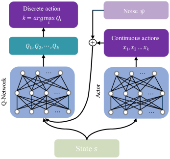
Figure 5: Illustration of the PDQN architecture.

For PDQN, the action space $\mathcal{A}$ consists of both continuous actions and discrete actions.

$$\mathcal{A}=\left\{(k,x_{k})|k\in K,x_{k}\in\mathcal{X}_{k}\right\}$$ (23)

where $K$ denotes the discrete action set, $k$ is a discrete action, $\mathcal{X}_{k}$ denotes the continuous action set, $x_{k}$ is a continuous action.

Inspired by the processing method of DQN, the actor network of PDQN uses the deterministic policy network $x(\cdot;\theta)$ to approximate $x_{k}$ in order to output continuous actions. The critic network approximate $Q(s,k,x_{k})$ with a deep neural network $Q(s,k,x_{k};\omega)$, thus outputting discrete actions.

Eq. (21) can be further expressed as:

$$\begin{split}Q(s,k,x_{k})=E[R_{t}+{\gamma}{\ \mathop{\rm max}\limits_{k\in K}Q(s^{\prime},k^{\prime},x_{k}(s^{\prime};\theta);\omega)}|s_{t}=s]\end{split}$$ (24)

The critic network parameters $\omega$ are updated based on the $TD$ error between $Q(s,k,x_{k};\omega)$ and the target network estimate $y$. PDQN performs the parameter update by minimizing the loss function, which is defined as the squared error between the target q-value and the estimated Q-value.

$$L_{Q}(\omega)={\frac{1}{2}}\Sigma(y-Q(s,k,x_{k};\omega))^{2}$$ (25)

where $y=R_{t}+{\gamma}{\rm max}_{k\in K}Q(s^{\prime},k^{\prime},x^{\prime}_{k};\omega)$.

The Actor network parameters $\theta$ is updated based on the negative sum of Q values.

$$L_{x}(\theta) =-\sum_{k=1}^{k}Q(s,k,x_{k}(s;\theta);\omega)$$ (26)

The target network is updated using the parameters of the actor and critic networks, and the update formula is as follows:

$$\omega_{i,targ} \leftarrow\tau{\omega_{i}}+(1-\tau){\omega_{i,targ}}$$ (27)

$$\theta_{i,targ} \leftarrow\tau{\theta_{i}}+(1-\tau){\theta_{i,targ}}$$ (28)

III-C PDQN-TD3 Algorithm

PDQN integrates DDPG and DQN, which can effectively solve continuous-discrete control problems. But PDQN also has the corresponding drawbacks of the two algorithms. PDQN algorithm involves a maximization operation when calculating the TD target, which leads to an overestimation of the true action value by PDQN. Additionally, due to the deep Q-network is continuously updated, eagerly updating value network parameter $\mu$ when the value network is still poor not only fails to improve $\mu$ but also destabilizes the training of the actor network due to the fluctuations in $\mu$. This paper applies a state-of-the-art PDQN-TD3 algorithm to solve the above problem.

PDQN-TD3 uses the actor-critic network architecture. The structure of the policy network and the evaluation network are designed using the TD3 structure. The policy network includes an actor network and the corresponding target network, while the evaluation network includes two critic networks and the corresponding target network. At each time step $t$, the environment feeds the state $s$ into the actor network of PDQN-TD3 to obtain the continuous action $x_{k}$. The critic network acts as a Q-value networks and select a discrete action $k$ based on the state variables and the output of the actor network using an $\epsilon$-greedy policy. After executing the continuous action and discrete action $(x_{k},k)$, the environment transitions to a new state $s_{t+1}$, and the tuple $(s,(x_{k},k),r,s_{t+1})$ is stored in the experience replay buffer for neural network training. Compared with PDQN, the PDQN-TD3 algorithm introduces three key techniques: clipped double-Q learning, delayed policy updates and target policy smoothing.

III-C1 Target policy smoothing

Random noise $\mathcal{N}(0,\sigma)$ obeying normal distribution was added to the target action value $\pi_{\phi_{targ}}(s)$ output by the actor network, and the noise value was limited within $(-c,c)$. It makes the update of the value function smooth and avoids overfitting.

$$\tilde{x}_{k} =\pi_{\phi_{targ}}(s)+clip(\mathcal{N}(0,\sigma),-c,c)$$ (29)

where $\tilde{x}_{k}$ is the action value after adding smooth noise.

III-C2 Clipped double-Q learning

To avoid overestimating the Q-function, PDQN-TD3 introduces two independent critic networks to learn the Q-function and construct the critic computing Q-target with smaller Q-value.

$$Q_{targ}(s^{\prime},k^{\prime},\tilde{x};\mu)={\rm min}_{i=1,2}Q_{targ}(s^{\prime},k^{\prime},\tilde{x};\mu_{i})$$ (30)

$$y=r+\gamma Q_{targ}(s^{\prime},k^{\prime},\tilde{x};\mu)$$ (31)

III-C3 Delayed policy updates

To enhance the stability of training the PDQN, the idea of delayed updates is introduced. The actor network is updated at a lower frequency, while the critic network is updated at a higher frequency. This approach ensures more stable training of the actor network.

The both critic network parameter updates is performed by minimizing the loss function, which is defined as the squared error between the target Q-value and the estimated Q-value.

$$L(\mu_{1})={\frac{1}{2}}\Sigma(y-Q(s,k,x_{k};\mu_{1}))^{2}$$ (32)

$$L(\mu_{2})={\frac{1}{2}}\Sigma(y-Q(s,k,x_{k};\mu_{2}))^{2}$$ (33)

The training process of PDQN-TD3 algorithm is shown in Algorithm 1.

Algorithm 1 PDQN-TD3 Algorithm Training Process.

  

  Initialization: Greedy algorithm coefficient $\varepsilon$ = 1, replay buffer $D$

  Random initialization: Online network parameters and target network parameters

  For: $t$ = 1: $T$ do

        Obtaining the initial state: $s(0)$

        Selecting a continuous action based on the current

   policy and exploration noise: $a_{t}=\pi_{\phi}(s_{t})+N(0,\sigma)$

        Selecting a discrete action based on the exploration

   policy:

$$\ \ k_{t}=\begin{cases}{\rm argmax}Q(\phi(s_{t}),k;\mu),1-\varepsilon\\ {\rm rand}(k_{t}),\varepsilon\end{cases}$$

        Executing a($t$) in the environment transitions

   to s($t+1$) and obtains r($t$)

        Saving the training sample sample(t) = s(t), a(t), r(t),

   s(t+1) in replay buffer $D$

        If: the replay buffer $D$ data is greater than 512

            Randomly selecting a mini-batch of samples

        (s(t), a(t), r(t), s(t+1)) from $D$

            Add noise to the actions in the sampled data:

        $\tilde{x}_{k}=\pi_{\phi_{targ}}(s)+clip(\mathcal{N}(0,\sigma),-c,c)$

            Calculate predicted value:

        $y=r+\gamma{\rm min}_{i=1,2}Q_{targ}(s^{\prime},k,\tilde{x}_{k};\theta_{t})$

            Update the critic network:

        $\mu_{t}\leftarrow{\rm argmin}_{\mu_{t}}N^{-1}\Sigma(y-Q(s,k,x_{k};\mu))^{2}$

            If: t mod d then:

                Update the actor network

                Update the target network

            End if

        End if

  End for

IV Energy Management Strategy via PDQN-TD3

IV-A Problem Description

The research object of this article is the DM-i series-parallel hybrid system. Due to the presence of both continuous control variables and discrete control variables, energy management systems are modeled as continuous-discrete action space. In this hybrid system, the PHEV series-parallel mode switching is achieved through the engagement/disengagement of the clutch, and the state of the clutch is a discrete variable. Therefore, the output torque of the engine is selected as the continuous action and the clutch engagement/disengagement as a discrete action.

IV-B The framework of PDQN-TD3 for EMS

This article proposes a HEV EMS based on continuous-discrete reinforcement learning PDQN-TD3, as shown in Fig. 6.

1) State: The state space of EMS based on PDQN-TD3 can be expressed as:

$$\begin{split}S=\left\{{SOC,v,P_{d}}\right\}\end{split}$$ (34)

2) Action: The action space can be expressed as:

$$\begin{split}A=\left\{{T_{e},i_{c}}\right\}\end{split}$$ (35)

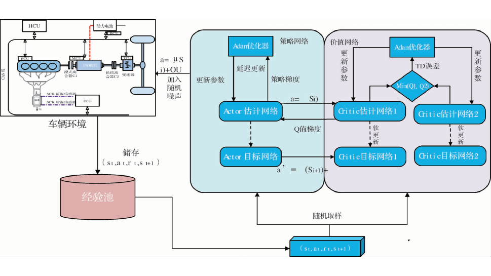
Figure 6: Energy management architecture based on PDQN-TD3 algorithm.

3) Reward: The primary goal of EMS is to minimize fuel and electricity consumption. Thus, the reward function is defined as the sum of fuel and electricity costs. To ensure that the agent does not violate the constraints of the hybrid power system during training, we also add a penalty term in the reward function for any violation of these constraints. The detailed reward function is defined as follows:

$$R=-(r_{c}+p_{\omega_{e}}+p_{soc})$$ (36)

$$r_{c}=(k_{f}\dot{m}_{f}+k_{e}\frac{P_{b}}{\eta_{b}\eta_{chr}})\Delta t$$ (37)

$$r_{\omega_{e}}=p_{\emph{m}ax}\Delta t$$ (38)

$$\ \ r_{soc}=\begin{cases}{0},\qquad&{\rm if}\;SOC_{l}\textless SOC\textless SOC_{h}\\ {p_{max}\frac{SOC-SOC_{h}}{1-SOC_{h}}},\qquad&{\rm if}\;SOC\textgreater SOC_{h}\\ {p_{max}\frac{SOC-SOC_{l}}{SOC_{l}}},\qquad&{\rm if}\;SOC\textless SOC_{l}\end{cases}$$ (39)

where $p_{\omega_{e}}$ and $p_{soc}$ are the penalties for exceeding the constraints on the engine angular velocity and SOC, respectively; $\Delta t=1s$; $k_{f}$ is the fuel price which is 7.6 CNY/L (10.3 CNY/kg); $k_{e}$ is the electric price which is 1.0 CNY/kW·h; $p_{max=}$ 0.1 is the maximum penalty, which is set to 10 times the maximum fuel consumption; The penalty for exceeding the SOC constraint is designed as a linear function of the SOC deviation from the desired range. Therefore, the greater the deviation of the SOC from the desired range, the higher the penalty.

V Simulation Analysis

V-A Simulation Parameters and Conditions

In order to verify the effectiveness and superiority of the proposed energy management method for HEVs, we conducted simulation experiments on the Python platform and compared it with EMS based on CD-CS and DP. The main hyperparameters of the PDQN-TD3 algorithm are shown in Table II. Three WLTC (Worldwide Light-duty Test Cycle) were selected as the simulation operating conditions. WLTC is chassis dynamometer tests for the determination of emissions and fuel consumption from light-duty vehicles. The total time for a complete WLTC cycle is 1800s, with a driving distance of 23.25 km, a maximum vehicle speed of 120 km/h, and an average vehicle speed of 31.51 km/h. The relationship between WLTC time and vehicle speed is shown in Fig. 7.

TABLE II: PDQN-TD3 Parameter

Parameter	Value
Soft target update	0.001
Reward discount factor	0.99
Actor network learning rate	0.0001
Q network learning rate	0.001
Experience replay memory size	200000
Mini-batch size	128
Action noise	N(0,0.02)
Actor network hidden layer size	64×64
Q network hidden layer size	64×64

Figure 7: Velocity profile of the driving cycle.

V-B DP-based energy management strategy

The DP is adopted as a global optimization algorithm for EMS. Under the premise that the entire driving cycle information is known in the future, the DP can obtain the optimal fuel economy. In order to investigate the optimization effect of the PDQN-TD3, this paper uses the DP as the benchmark for fuel economy. For DP, as the driving conditions serve as prior knowledge, the future vehicle speed and power demand are both known. At this point, SOC serves as the only state variable in the system. As the clutch switch only considers two states of engagement and disengagement, the clutch switch state is divided into two grids when performing DP. Simulation analysis shows that increasing the number of grids for engine torque and battery SOC after a certain amount does not significantly reduce the cost function of the system but does increase the computation time of the DP when the engine torque and battery SOC are discretized. Therefore, in this paper, SOC is divided into 60 grids in the range of 0.3 to 0.9, while the engine torque is divided into 120 grids in the range of 0 - 120N. In the simulation process, we use the general DP Matlab toolbox [30] to obtain the benchmark.

V-C Rule-based energy management strategy

The rule-based control strategy selects the optimal operation mode based on predetermined judgment conditions and control logic. It has the advantages of simplicity and easy implementation, making it a widely adopted EMS by automotive companies. To compare the fuel-saving effect of PDQN-TD3, this paper has designed a rule-based EMS. Specifically, rule-based EMS are mainly divided into two modes: CD and CS mode.

SOC $>$ 0.3, the vehicle enters CD mode.

(1) When the vehicle demand torque $T_{d}$ is greater than the engine optimal working point:

① If $v\geq$ 60: When $T_{d}$ is greater than the engine maximum working point $T_{e\_max}$, the vehicle enters the series mode, otherwise it enters the parallel mode.

② If $v<$ 60, the vehicle enters the series mode.

(2) When $T_{d}$ is less than the engine optimal working point:

① If $T_{d}<$ 0: When SOC $>$ 0.9, mechanical braking is used; otherwise, energy is recovered by driving motor.

② If $T_{d}>$ 0, the vehicle enters EV mode.

SOC $<$ 0.3, the vehicle enters CS mode.

(1) When $T_{d}>T_{e\_min}$:

① If $T_{d}>T_{e\_max}$, then $T_{e}=T_{e\_max}$. If $v>$ 60, the vehicle enters the engine direct drive mode, otherwise it enters the series mode.

② When $T_{d}<T_{e\_max}$: if $v>$ 60, the vehicle enters the engine direct drive mode. Otherwise, the vehicle enters the series mode.

(2) When $T_{d}<T_{e\_min}$: the vehicle enters the series mode.

(3) If $T_{d}<$ 0, energy is recovered through the driving motor.

For the above rules:

(1) In series mode, the clutch is disengaged, the engine works in the optimal economic range to drive the generator for power generation, while the motor provides the demand torque.

(2) In parallel mode, the clutch is engaged, the generator does not work, the motor aids the engine to drive the vehicle.

(3) In EV mode, the clutch is disengaged, neither the engine nor the generator works, and the motor provides the demand torque.

(4) In engine direct drive mode, the clutch is engaged, the generator does not work, and the engine directly drives the vehicle.

V-D Simulation Result Analysis

As shown in Fig. 8, the curve represents the cumulative reward changes, where a higher return value indicates a better learning effect. It can be observed that the return value curve fluctuates but exhibits an overall upward trend, indicating that the intelligent agent continuously adjusts its strategy to obtain the maximum cumulative return per episode. After $18\times 10^{4}$ steps iteration, the algorithm gradually converges to the optimal control strategy. The PDQN-TD3 and the DP-based strategy have similar total energy consumption, indicating that the PDQN-TD3 control strategy has better fuel economy.

The comparison of the vehicle SOC variation trends over time for three algorithms under the WLTC cycle is shown in Fig. 9. It can be observed that the CD-CS strategy tends to use electric energy rather than engine energy when the battery SOC is greater than $\rm SOC_{min}$. When the battery SOC drops to the set threshold, the SOC fluctuates around $\rm SOC_{min}$, and the engine becomes the main power source to suppress excessive discharge of the battery. However, using this control strategy under aggressive driving conditions requires the engine to provide significant torque output when the battery is depleted, which reduces the fuel economy of the vehicle. On the other hand, the variation trend generated by the PDQN-TD3 and DP algorithms is very similar, but the SOC decrease of the PDQN-TD3 is more gradual. This indicates that when the PDQN-TD3 performs energy management, the frequency of engine startup to charge the battery will increase compared to the DP under the same driving conditions. This will reduce the peak discharge power of the power battery, which is positive and beneficial for the battery’s lifespan. Compared with CD-CS, the motor can provide greater output power under aggressive driving conditions, and the engine working point can be adjusted more reasonably to allow the engine to work more often in the optimal fuel economy range.

Figure 8: Episode reward sum in training.

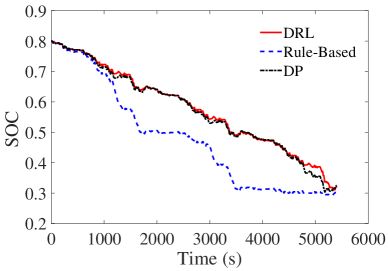
Figure 9: Battery SOC trajectories under different EMSs.

Table III shows the simulation results of the total system energy consumption for fuel and electricity consumption. As can be seen from Table III, the DP-based achieves optimal fuel economy, which we use as a benchmark for comparison with the PDQN-TD3 and CD-CS methods. The PDQN-TD3 EMS improves fuel economy by 10.08% compared to the CD-CS EMS. The fuel economy gap between PDQN-TD3 EMS and DP is 6%. This indicates that PDQN-TD3 has a better energy utilization efficiency, which reduces the operating costs of HEVs, further demonstrating the optimality of the PDQN-TD3 strategy for energy management.

TABLE III: Comparison Analysis of Total Cost in Different Methods

Algorithm	total cost/CNY	fuel consumption/100km	gap
PDQN-TD3	13.29	1.84	6.24%
CD-CS	14.78	2.01	18.15%
DP	12.51	1.68	0%

Fig. 10 to Fig. 12 show the engine operating points for the three control strategies. It can be seen that the EMS based on DP has more engine operating points in the fuel-efficient range. The main reason for the sparse distribution of engine operating points is that DP discretizes the engine torque, and due to the influence of the discretization precision, the engine operating point can only be selected from discrete intervals and limited discrete engine operating points on the map. Therefore, one point on the map may correspond to many engine torques with the same value. Although DP has better optimization results, its computation time is longer than that of PDQN-TD3 and CD-CS, which is the main reason why the DP algorithm cannot be applied to real vehicles. Compared with the EMS based on CD-CS, the control strategy based on PDQN-TD3 has smaller fluctuations in engine speed and torque, which further indicates that the EMS based on PDQN-TD3 can adjust the engine operating point well, so that the engine can work in the optimal fuel economy zone in most cases. Compared with CD-CS, the engine operates more efficiently and the vehicle has better fuel economy. The reason why the engine in CD-CS works in a non-economical range is that when the battery SOC is lower than $\rm SOC_{min}$, the output power of the battery is restricted and cannot even provide power to the outside. At this time, the vehicle can only be driven by the engine, which to some extent limits the engine’s efficiency and reduces fuel economy.

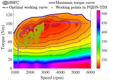
Figure 10: Engine working points of PDQN-TD3.

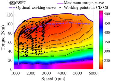
Figure 11: Engine working points of CD-CS.

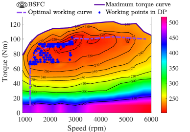
Figure 12: Engine working points of DP.

Fig. 13 to Fig. 15 show the operating points of the three control strategies for the electric motor. It can be seen that for PDQN and DP algorithms, EV mode is mainly distributed in the area of low vehicle speeds. As the vehicle speed further increases, the engine starts, and the system operates in HEV mode. Different from DP and PDQN, for the CDCS control strategy, the system will also frequently enter the HEV mode when the vehicle speed is very low. This is because when the battery power is depleted, the battery cannot meet the power demand of the system and has to rely on the engine generation to provide additional power frequently. However, DP and PDQN can plan the battery usage more reasonably by driving the vehicle using the engine at higher speeds. This not only improves fuel economy but also reduces the output torque of the motor, which is beneficial for the battery’s lifespan.

From Fig. 16, it can be seen that compared to the PDQN and DP strategies, the CD-CS strategy has a lower frequency of operation in the EV mode and a significantly higher frequency in the HEV mode. This is because, for the CD-CS control strategy, even when the battery is fully charged, the vehicle may still operate in the EV mode even if the vehicle speed is high or the torque demand is large at the current moment. This undoubtedly increases the instantaneous power of the power battery, leading to a faster decline in battery capacity and potentially harming its health and lifespan. When the battery SOC drops to a set threshold, the battery is unable to provide sufficient driving torque and cannot enter the EV mode at low speeds, forcing the engine to start frequently in non-economical regions, which undoubtedly increases fuel consumption.

Figure 13: Motor working woints of PDQN-TD3.

Figure 14: Motor working points of CD-CS.

Figure 15: Motor working points of DP.

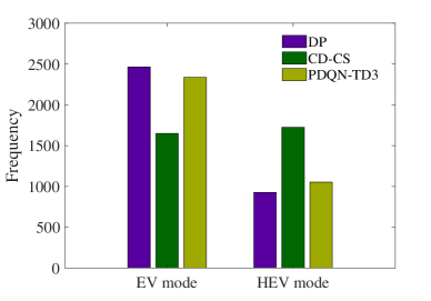
Figure 16: Operating times of EV and HEV modes by different EMSs.

Fig. 17 show the engagement/disengagement of the clutch under three different control strategies. The statistical results of the clutch engagement/disengagement are presented in Table IV. It can be seen that for all three control strategies, the clutch disengagement times are greater than the clutch engagement times. This is because the cost of electricity is lower than the cost of fuel, although direct drive of the engine is more economical when the clutch is engaged, it cannot guarantee that the engine operates in the economic range at low speed or low torque. Instead, it increases fuel consumption. In this case, the system still tends to generate electricity through the engine in the high-efficiency range rather than directly driving the vehicle. The difference between the three strategies is that the CD-CS has significantly fewer clutch engagements. This is because at the beginning of the journey, the CD-CS tends to use electricity, and the engine is almost not started until the system’s torque demand or vehicle speed exceeds the set threshold. When the SOC of the battery is low, although the engine needs to be started frequently to provide torque, because the system does not have a transmission, the engine cannot directly drive the vehicle at any speed. More often, the engine acts as a range extender. The number of clutch engagements in PDQN-TD3 and DP differs by 2.8%, which may be due to the lower fuel efficiency of PDQN-TD3 than DP. PDQN-TD3 can’t predict the operating conditions of the entire journey in advance like DP, which may limit the optimization effect of PDQN-TD3 to some extent.

TABLE IV: The Statistical Results of the Clutch Engagement/Disengagement

Algorithm	Clutch engagement period percentage
CD-CS	8.62%
PDQN-TD3	16.66%
DP	17.14 %

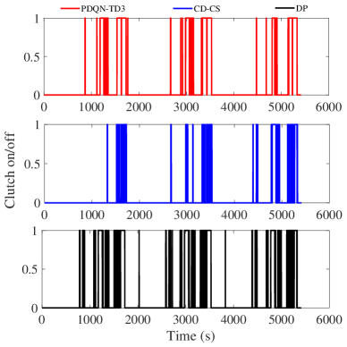
Figure 17: Clutch engagement/disengagement signal.

VI Conclusions

This work focuses on the BYD DM-i hybrid system and conducts mathematical modeling of the hybrid system and energy management optimal control. The main conclusions are as follows:

Considering the characteristics of the hybrid system with both continuous and discrete variables, we establish a control-oriented mathematical model for the DM-i hybrid systems from the perspective of mixed-integer programming. This enables the simultaneous handling of both continuous and discrete variables in energy management problems.

The continuous-discrete RL algorithm PDON-TD3 was applied to energy management, achieving simultaneous optimization of both continuous (engine torque) and discrete action (clutch switch). The PDQN-TD3 EMS has better fuel economy and emission reduction effects compared to the CD-CS, with a 10.08% reduction in the total cost of fuel consumption and electric energy consumption. The cost effectiveness gap of the PDQN-TD3 method is 6.4% compared with DP, and it has greater potential for real-time online application. This method can achieve energy-saving driving without compromising vehicle performance.

Future research can explore the integration of prediction mechanisms into RL algorithms, further improving the energy utilization efficiency and driving comfort of HEVs. In addition, the cooperative optimization of energy management and advanced driving assistance systems for HEV is also possible future work for energy saving and emission reduction.

References

- [1] J. Torres, R. Gonzalez, A. Gimenez, and J. Lopez, “Energy management strategy for plug-in hybrid electric vehicles. a comparative study,” Applied Energy, vol. 113, pp. 816–824, 2014.
- [2] V. A. Katkar and P. Goswami, “Review on energy management systems for hybrid e vehicles,” in 2020 International Conference on Power, Energy, Control and Transmission Systems (ICPECTS). IEEE, 2020, pp. 1–6.
- [3] C.-C. Lin, H. Peng, J. W. Grizzle, and J.-M. Kang, “Power management strategy for a parallel hybrid electric truck,” IEEE Transactions on Control Systems Technology, vol. 11, no. 6, pp. 839–849, 2003.
- [4] V. Navale and T. C. Havens, “Fuzzy logic controller for energy management of power split hybrid electrical vehicle transmission,” in 2014 IEEE International Conference on Fuzzy Systems (FUZZ-IEEE). IEEE, 2014, pp. 940–947.
- [5] T. Liu, W. Tan, X. Tang, J. Zhang, Y. Xing, and D. Cao, “Driving conditions-driven energy management strategies for hybrid electric vehicles: A review,” Renewable and Sustainable Energy Reviews, vol. 151, p. 111521, 2021.
- [6] X. Lin, K. Li, and L. Wang, “A driving-style-oriented adaptive control strategy based pso-fuzzy expert algorithm for a plug-in hybrid electric vehicle,” Expert Systems with Applications, vol. 201, p. 117236, 2022.
- [7] L. Li, S. You, C. Yang, B. Yan, J. Song, and Z. Chen, “Driving-behavior-aware stochastic model predictive control for plug-in hybrid electric buses,” Applied Energy, vol. 162, pp. 868–879, 2016.
- [8] Z. Yuan, L. Teng, S. Fengchun, and H. Peng, “Comparative study of dynamic programming and pontryagin’s minimum principle on energy management for a parallel hybrid electric vehicle,” Energies, vol. 6, no. 4, pp. 2305–2318, 2013.
- [9] A. Brahma, Y. Guezennec, and G. Rizzoni, “Optimal energy management in series hybrid electric vehicles,” in Proceedings of the 2000 American Control Conference. ACC (IEEE Cat. No. 00CH36334), vol. 1, no. 6. IEEE, 2000, pp. 60–64.
- [10] C. Zheng, G. Xu, S.-W. Cha, and Q. Liang, “Numerical comparison of ecms and pmp-based optimal control strategy in hybrid vehicles,” International Journal of Automotive Technology, vol. 15, pp. 1189–1196, 2014.
- [11] P. Saiteja and B. Ashok, “Critical review on structural architecture, energy control strategies and development process towards optimal energy management in hybrid vehicles,” Renewable and Sustainable Energy Reviews, vol. 157, p. 112038, 2022.
- [12] R. Schmid, J. Bürger, and N. Bajcinca, “A comparison of pmp-based energy management strategies for plug-in-hybrid electric vehicles,” IFAC-PapersOnLine, vol. 52, no. 5, pp. 592–597, 2019.
- [13] N. Kim, S. Cha, and H. Peng, “Optimal control of hybrid electric vehicles based on pontryagin’s minimum principle,” IEEE Transactions on Control Systems Technology, vol. 19, no. 5, pp. 1279–1287, 2010.
- [14] L. Guo, B. Gao, Y. Gao, and H. Chen, “Optimal energy management for hevs in eco-driving applications using bi-level mpc,” IEEE Transactions on Intelligent Transportation Systems, vol. 18, no. 8, pp. 2153–2162, 2016.
- [15] S. Yang, W. Wang, F. Zhang, Y. Hu, and J. Xi, “Driving-style-oriented adaptive equivalent consumption minimization strategies for hevs,” IEEE Transactions on Vehicular Technology, vol. 67, no. 10, pp. 9249–9261, 2018.
- [16] G. Jinquan, H. Hongwen, P. Jiankun, and Z. Nana, “A novel mpc-based adaptive energy management strategy in plug-in hybrid electric vehicles,” Energy, vol. 175, pp. 378–392, 2019.
- [17] A. Rezaei, J. B. Burl, and B. Zhou, “Estimation of the ecms equivalent factor bounds for hybrid electric vehicles,” IEEE Transactions on Control Systems Technology, vol. 26, no. 6, pp. 2198–2205, 2017.
- [18] X. Qi, G. Wu, K. Boriboonsomsin, and M. J. Barth, “A novel blended real-time energy management strategy for plug-in hybrid electric vehicle commute trips,” in 2015 IEEE 18th International Conference on Intelligent Transportation Systems. IEEE, 2015, pp. 1002–1007.
- [19] S. A. Kouche-Biyouki, S. M. A. Naseri-Javareshk, A. Noori, and F. Javadi-Hassanehgheh, “Power management strategy of hybrid vehicles using sarsa method,” in Electrical Engineering (ICEE), Iranian Conference on. IEEE, 2018, pp. 946–950.
- [20] Y. Lin, J. McPhee, and N. L. Azad, “Co-optimization of on-ramp merging and plug-in hybrid electric vehicle power split using deep reinforcement learning,” IEEE Transactions on Vehicular Technology, vol. 71, no. 7, pp. 6958–6968, 2022.
- [21] D. Xu, C. Zheng, Y. Cui, S. Fu, N. Kim, and S. W. Cha, “Recent progress in learning algorithms applied in energy management of hybrid vehicles: a comprehensive review,” International Journal of Precision Engineering and Manufacturing-Green Technology, vol. 10, no. 1, pp. 245–267, 2023.
- [22] N. P. Farazi, B. Zou, T. Ahamed, and L. Barua, “Deep reinforcement learning in transportation research: A review,” Transportation Research Interdisciplinary Perspectives, vol. 11, p. 100425, 2021.
- [23] J. Wu, H. He, J. Peng, Y. Li, and Z. Li, “Continuous reinforcement learning of energy management with deep q network for a power split hybrid electric bus,” Applied Energy, vol. 222, pp. 799–811, 2018.
- [24] X. Han, H. He, J. Wu, J. Peng, and Y. Li, “Energy management based on reinforcement learning with double deep q-learning for a hybrid electric tracked vehicle,” Applied Energy, vol. 254, p. 113708, 2019.
- [25] F. Chen, P. Mei, H. Xie, S. Yang, B. Xu, and C. Huang, “Reinforcement learning-based energy management control strategy of hybrid electric vehicles,” in 2022 8th International Conference on Control, Automation and Robotics (ICCAR). IEEE, 2022, pp. 248–252.
- [26] J. Zhou, S. Xue, Y. Xue, Y. Liao, J. Liu, and W. Zhao, “A novel energy management strategy of hybrid electric vehicle via an improved td3 deep reinforcement learning,” Energy, vol. 224, p. 120118, 2021.
- [27] Y. Li, H. He, A. Khajepour, H. Wang, and J. Peng, “Energy management for a power-split hybrid electric bus via deep reinforcement learning with terrain information,” Applied Energy, vol. 255, p. 113762, 2019.
- [28] H. Zhang, J. Peng, H. Tan, H. Dong, and F. Ding, “A deep reinforcement learning-based energy management framework with lagrangian relaxation for plug-in hybrid electric vehicle,” IEEE Transactions on Transportation Electrification, vol. 7, no. 3, pp. 1146–1160, 2020.
- [29] X. Tang, J. Chen, H. Pu, T. Liu, and A. Khajepour, “Double deep reinforcement learning-based energy management for a parallel hybrid electric vehicle with engine start–stop strategy,” IEEE Transactions on Transportation Electrification, vol. 8, no. 1, pp. 1376–1388, 2021.
- [30] O. Sundstrom and L. Guzzella, “A generic dynamic programming matlab function,” in 2009 IEEE Cntrol Applications,(CCA) & Intelligent Control,(ISIC). IEEE, 2009, pp. 1625–1630.