Deep imaging inside scattering media through virtual spatiotemporal wavefront shaping

Abstract

The multiple scattering of light makes materials opaque and obstructs imaging. Wavefront shaping can reverse the scattering process, but imaging with physical wavefront shaping has severe deficiencies such as requiring physical guidestars, limited within a small isoplanatic patch, restricted to planar targets outside the scattering media, and slow wavefront updates due to the hardware. Here, we introduce scattering matrix tomography (SMT): measure the hyperspectral scattering matrix of the sample, use it to digitally scan a synthesized confocal spatiotemporal focus and construct a volumetric image of the sample, and then use the synthesized image as many virtual guidestars to digitally optimize the pulse shape, input wavefront, and output wavefront to compensate for aberrations and scattering. The virtual feedback dispenses with physical guidestars and enables hardware-free spatiotemporal wavefront corrections across arbitrarily many isoplanatic patches. We demonstrate SMT with sub-micron diffraction-limited lateral resolution and one-micron bandwidth-limited axial resolution at one millimeter beneath ex vivo mouse brain tissue and inside a dense colloid, where all existing imaging methods fail due to the overwhelming multiple scattering. SMT translates imaging and wavefront shaping into a computational problem. It is noninvasive and label-free, provides multi-isoplanatic volumetric images inside and outside the scattering media, and can be applied to medical imaging, device inspection, biological science, and colloidal physics.

I Introduction

Light scattering from inhomogeneities scrambles the wavefront and attenuates the signal exponentially while obscuring it with a speckled multiple-scattering background, making it a challenge to image ^{1, 2}. Achieving diffraction-limited resolution deep inside disordered media like biological tissue and colloidal suspension is a long-sought-after goal that can enable through-skull optical imaging and stimulation, biopsy-free pathology, observation of cellular processes in their natural state, optical characterization of bulk colloids, high-resolution nondestructive device testing, and many other applications.

Traditional imaging methods work by filtering away the multiple-scattering background to reveal the exponentially small unscattered signal. The reflectance confocal microscopy (RCM) ^{3, 4} uses spatial gating. Optical coherence tomography (OCT) ⁵ applies a coherence gate. The axial span of the spatial beam (which is twice the Rayleigh range) must cover the axial span of the image (i.e., the depth of field $\Delta z$), so OCT operates with a small numerical aperture (NA), leading to a coarse lateral resolution (typically 5–20 µm). Optical coherence microscopy (OCM) ⁶ combines spatial filtering and coherence gating while trading off the depth of field. Interferometric synthetic aperture microscopy ⁷ extends the depth of field, though its signal decreases with the loss of confocal gates away from the focal plane. Hardware ⁸ and computational ^{9, 10, 11} adaptive optics can correct for wavefront distortions to improve the image, but the improvement is limited by the number of elements on the correction device. Multiphoton microscopy adopts longer wavelengths where scattering is weaker but requires fluorescence labeling and high-power lasers ^{12, 13}. Tomographic phase microscopy quantitatively obtains the refractive index distribution ^{14, 15, 16, 17, 18} but only works for thin specimens and requires access to both sides of the sample for transmission measurements. Selective detection of the forward scattered photons ^{19, 20} and photoacoustic tomography ²¹ allow imaging deeper at reduced resolution. Despite these developments, the depth-over-resolution ratio stays around or below 200 in biological tissue across existing label-free imaging methods (including non-optical ones such as ultrasound, X-ray CT, and MRI) ^{21, 22, 23}.

In recent years, a paradigm shift came with the appreciation that light scattering is deterministic and controllable. Given enough control elements, a suitable incident wavefront can reverse the multiple scattering process ^{24, 25} thanks to the time-reversal symmetry of Maxwell’s equations. Adopting such wavefronts can, in principle, allow imaging at much deeper depths. But current methods to determine these special wavefronts come with severe limitations as they introduce physical guidestars at the imaging site ²⁶ such as invasive cameras ^{27, 28} or photorefractive crystals ^{29, 30}, fluorescence labels ^{31, 32, 33}, acoustic foci with greatly reduced spatial resolution ^{34, 35}, or isolated moving particles ^{36, 37}. Additionally, each wavefront is only valid within a volume called the isoplanatic patch ⁸, whose size shrinks with depth and is less than 10 µm at 1 mm deep inside biological tissue ^{38, 39}, gravely restricting the field of view. Such physical-guidestar-based schemes are schematically illustrated in Fig. 1a. To avoid using physical guidestars, researchers developed incoherent imaging methods based on angular correlations ^{40, 41} and optimization ^{42, 43}. However, they only considered planar targets far outside the scattering media since the imaging volume is still limited by the isoplanatic patch size. Reflection matrix measurement is another way to avoid physical guidestars. One can accumulate single-scattering signals using correlations in the reflection matrix ⁴⁴ and remove aberrations and scattering through singular value decomposition ^{45, 46} or iterative phase conjugation ^{47, 48, 49, 50, 51, 52}, culminating in the “volumetric reflection-matrix microscopy” (VRM) method ⁵² that performs both spectral and angular corrections. These matrix-based methods show great potential but, to date, have yet to deliver the drastic beyond-adaptive-optics scattering compensation promised by wavefront shaping.

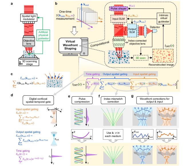
Fig. 1: Virtual spatiotemporal wavefront shaping and scattering matrix tomography (SMT). a, Imaging with wavefront modulated by physical lenses and spatial light modulators (SLMs) using feedback from artificially introduced physical guidestars. b, SMT imaging with virtual wavefront shaping that digitally performs spatiotemporal wavefront modulation, volumetric scanning, and optimization via Eqs. (2)–(3). The reconstructed image acts as virtual guidestars intrinsic to the sample, providing feedback noninvasively. c, The scattering matrix $S(\bf k_{\rm out},\bf k_{\rm in},\omega)$ relates any incident field $\tilde{E}_{\rm in}(\bf k_{\rm in},\omega)$ to the resulting scattered field $\tilde{E}_{\rm out}(\bf k_{\rm out},\omega)$. d, The scattering matrix can synthesize input spatial gating, output spatial gating, and time gating by summing over the incident momentum ${\bf k}_{\rm in}$, outgoing momentum ${\bf k}_{\rm out}$, and frequency $\omega$ respectively. e–g, Dispersion, refractive index mismatch at interfaces, and wavefront distortions (from both the optical system and the sample, including both aberrations and multiple scattering) degrade the gates. SMT corrects all of them digitally through a frequency-dependent phase $\theta(\omega)$ that acts as a virtual pulse shaper, appropriate momenta and phase coefficients for the medium that act as a virtual index-corrected objective lens, and angle-dependent phases $\phi_{\rm in}(\bf k_{\rm in})$ and $\phi_{\rm out}(\bf k_{\rm out})$ that act as two virtual SLMs.

It would be ideal if one could combine the noninvasive confocal spatial and temporal gating of the traditional label-free imaging methods with the scattering compensation offered by wavefront shaping while avoiding the restrictions of physical guidestars, overcoming the isoplanatic patch size limit, allowing volumetric imaging inside the scattering media, and significantly outperforming conventional adaptive optics. Here we enable all of these through “virtual wavefront shaping” (Fig. 1b). We measure the hyperspectral scattering matrix of the sample and use it to synthesize a spatiotemporal focus with wavefront correction for every isoplanatic patch, pulse compression, and refractive index mismatch correction. We scan the focus digitally to yield a phase-resolved 3D image of the sample with no depth-of-field trade-off. The reconstructed image acts as virtual guidestars intrinsic to the sample, and we develop an optimization with regularization and progression strategies to find the optimal dispersion compensation and input/output wavefronts. This led to a depth-over-resolution ratio of 910 when imaging a resolution target at one millimeter beneath ex vivo mouse brain tissue—the highest ratio reported in the literature (including all optical and all non-optical label-free methods) to our knowledge. We attain ideal diffraction-limited resolution when the signal is reduced by over ten-million-fold due to multiple scattering, where all other methods fail. We maintain the ideal transverse and axial resolutions across a depth of field of over 70 times the Rayleigh range deep inside a dense colloid. This approach converts the problem of imaging and reversing light scattering to a reconstruction and optimization problem, where physics and computation can push the frontier of imaging depth.

II Scattering matrix tomography

The scattering matrix $S(\bf k_{\rm out},\bf k_{\rm in},\omega)$ encapsulates the sample’s complete linear response ^{53, 54} (Fig. 1c). Any incident wave is a superposition of plane waves: ${\it E}_{\rm in}({\bf r},t)=\sum_{{\bf k}_{\rm in},\omega}\tilde{\it E}_{\rm in}({\bf k}_{\rm in},\omega)e^{i{\bf k}_{\rm in}\cdot{\bf r}-i\omega t}$, where ${\bf r}=(x,y,z)$ is the position, $t$ is time, and $\tilde{\it E}_{\rm in}({\bf k}_{\rm in},\omega)$ is the amplitude of its plane-wave component with incoming momentum $\bf k_{\rm in}$ at frequency $\omega$. The amplitudes $\tilde{E}_{\rm out}({\bf k}_{\rm out},\omega)$ that form the resulting outgoing wave ${\it E}_{\rm out}({\bf r},t)=\sum_{{\bf k}_{\rm out},\omega}\tilde{\it E}_{\rm out}({\bf k}_{\rm out},\omega)e^{i{\bf k}_{\rm out}\cdot{\bf r}-i\omega t}$ are given by the scattering matrix through $\tilde{E}_{\rm out}({\bf k}_{\rm out},\omega)=\sum_{{\bf k}_{\rm in}}S({\bf k}_{\rm out},{\bf k}_{\rm in},\omega)\tilde{E}_{\rm in}(\bf k_{\rm in},\omega)$. The angular summations are restricted to $|{\bf k}|^{2}=|{\bf k}_{\parallel}|^{2}+k_{z}^{2}=(n_{\rm bg}\omega/c)^{2}$ in a background medium with speed of light $c/n_{\rm bg}$; we use “angle” interchangeably with “momentum.”

After measuring a subset of $S(\bf k_{\rm out},\bf k_{\rm in},\omega)$, we can digitally synthesize the sample’s response with tailored measurements in space-time given customized spatiotemporal inputs, which we collectively refer to as “virtual spatiotemporal wavefront shaping.” As illustrated in Fig. 1d, summing over incident angles $\bf k_{\rm in}$ with incoming plane-wave amplitudes $\tilde{E}_{\rm in}({\bf k}_{\rm in},\omega)=e^{-i{\bf k_{\rm in}}\cdot{\bf r_{\rm in}}}$ creates an incident beam ${\it E}_{\rm in}({\bf r},\omega)$ spatially focused at $\bf r_{\rm in}$, forming an input spatial gate; summing over outgoing angles $\bf k_{\rm out}$ with outgoing plane-wave amplitudes $\tilde{E}_{\rm out}({\bf k}_{\rm out},\omega)$ from the scattering matrix yields the scattered field ${\it E}_{\rm out}({\bf r}={\bf r}_{\rm out},\omega)$ given a virtual detector at position ${\bf r}_{\rm out}$, forming an output spatial gate; summing over frequency $\omega$ with an $e^{-i\omega(t-t_{0})}$ phase creates an incident pulse that arrives at $\bf r_{\rm in}$ at time $t=t_{0}$, forming a temporal gate. Given a spatiotemporal focus arriving at $\bf r_{\rm in}$ at time $t_{0}$, the scattered field is therefore $E_{\rm out}({\bf r}_{\rm out},\it t)=\sum_{\bf k_{\rm out},\bf k_{\rm in},\omega}S({\bf k}_{\rm out},{\bf k}_{\rm in},\omega)e^{i{\bf k}_{\rm out}\cdot{\bf r}_{\rm out}-i{\bf k}_{\rm in}\cdot{\bf r}_{\rm in}-i\omega(t-t_{0})}$. Aligning the input spatial gate with the output spatial gate (setting ${\bf r}_{\rm in}={\bf r}_{\rm out}={\bf r}$) and then aligning the temporal gate with the two spatial gates (evaluating $E_{\rm out}$ at time $t=t_{0}$), we obtain the triply-gated scattering amplitude of the sample at position ${\bf r}$, denoted as

$$\psi_{\rm SMT}(\bf r)=\sum_{\bf k_{\rm out},\bf k_{\rm in},\omega}\it e^{\it i(\bf k_{\rm out}-\bf k_{\rm in})\cdot{\bf r}}\it S(\bf k_{\rm out},\bf k_{\rm in},\omega).$$ (1)

Digitally scanning $\bf{r}$ (Fig. 1b) forms a phase-resolved image of the sample where the input spatial gate, output spatial gate, and temporal gate all align at every point in the absence of scattering. The lateral spread of $\bf k_{\rm out}-\bf k_{\rm in}$ in the summation (typically set by the NA) determines the lateral resolution, not restricted to any focal plane. The axial spread (typically set by the spectral bandwidth) determines the axial resolution. The $\psi_{\rm SMT}(\bf r)$ image can be volumetric or a slice with any orientation. The triple summation averages away random noises, providing a signal-to-noise ratio advantage akin to that of frequency-domain OCT over time-domain OCT ⁵⁵. One can utilize any subset of the scattering matrix—reflection, transmission, remission ^{19, 56}, a combination of them, or other subsets—with any number of angles and frequencies. We use the non-uniform fast Fourier transform ⁵⁷ to efficiently evaluate these summations and the 3D spatial scan. Eq. (1) is the minimal, optimization-free version of what we call “scattering matrix tomography” (SMT).

SMT efficiently suppresses multiple scattering. The single-scattering field at output ${\bf k}_{\rm out}$ for an input from ${\bf k}_{\rm in}$ is given by the Born approximation as proportional to $\tilde{\eta}({\bf q})$, namely the ${\bf q}={\bf k}_{\rm out}-{\bf k}_{\rm in}$ component of the 3D Fourier transform of the sample’s permittivity contrast profile $\eta({\bf r})$ ^{58, 14, 15}. Such single-scattering contributions add up in phase in Eq. (1) to form the image, similar to an inverse Fourier transform from $\tilde{\eta}({\bf q})$ to $\eta({\bf r})$. The multiple-scattering contributions do not add up in phase. Therefore, the triple summations over $\bf k_{\rm out}$, $\bf k_{\rm in}$, and $\omega$ boost the single-to-multiple-scattering ratio in $\psi_{\rm SMT}$ to enable imaging even when multiple scattering is orders of magnitude stronger than single scattering in the raw measurement data $S({\bf k}_{\rm out},{\bf k}_{\rm in},\omega)$.

To further compensate for aberrations and scattering, we perform digital spatiotemporal wavefront corrections. The chromatic aberrations in the optical elements of the system and the frequency dependence of the refractive index in the sample create a frequency-dependent phase that misaligns and broadens the temporal gate. In SMT, we digitally compensate for such dispersion using a spectral phase $\theta(\omega)$, acting as a virtual pulse shaper (Fig. 1e). The refractive index mismatch between the sample medium (e.g., biological tissue), the far field (e.g., air), and the coverslip (if there is one) refracts the rays, degrades the input and output spatial gates ⁵⁹, and misaligns the spatial gates and the temporal gate. By using the appropriate propagation phase shift $(\bf k_{\rm out}-\bf k_{\rm in})\cdot{\bf r}$ in each medium and setting the optimal temporal gate, SMT achieves an ideal spatiotemporal focus at all depths even in the presence of refraction, effectively creating a virtual dry objective lens that reverses both the spatial and the chromatic aberrations arising from the index mismatch (Fig. 1f) without liquid immersion (Supplementary Sect. III C). Importantly, we also digitally introduce angle-dependent phase profiles $\phi_{\rm in}(\bf k_{\rm in})$ and $\phi_{\rm out}(\bf k_{\rm out})$ that act as two virtual spatial light modulators (SLMs), one for the incident wave and one for the outgoing wave (Fig. 1g), which can adopt any wavefront to compensate for additional aberrations and scattering. This yields the general form of SMT,

$$I_{\rm SMT}(\bf{r})\it= \left|\sum_{\omega}e^{i\theta(\omega)}\sum_{\bf k_{\rm out}}e^{i\bf k_{\rm out}\cdot\bf{r}+\it i\phi_{\rm out}(\bf k_{\rm out})}\right.$$

$$\,\,\left.\sum_{\bf k_{\rm in}}e^{-i\bf k_{\rm in}\cdot\bf{r}+\it i\phi_{\rm in}(\bf k_{\rm in})}S(\bf k_{\rm out},\bf k_{\rm in},\omega)\right|^{2}.$$ (2)

By measuring the diagonal elements of the scattering matrix of a mirror, we remove the dispersion and most input aberrations in the optical system (Supplementary Sect. III B).

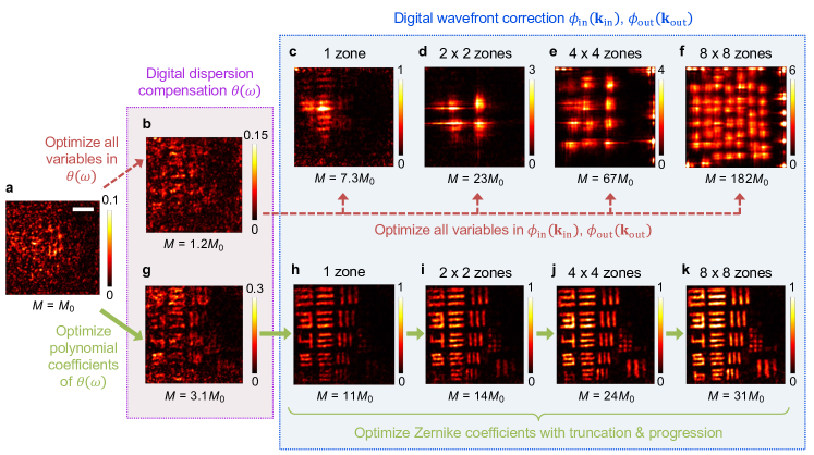
Fig. 2: SMT digital dispersion compensation and wavefront corrections. SMT finds the digital corrections $\theta(\omega)$, $\phi_{\rm in}(\bf k_{\rm in})$, and $\phi_{\rm out}(\bf k_{\rm out})$ by optimizing an image quality metric $M$, Eq. (3). Different spatial zones of the image use different $\phi_{\rm in/out}$. Each panel shows the SMT image $I_{\rm SMT}({\bf r})$ of the USAF-target-under-tissue sample of Fig. 4 in this process, at the depth where $M$ is maximized. A direct optimization (red dashed arrows) leads to overfitting and gets trapped in poor local optima. Through regularization and progression strategies described in the text (green solid arrows), SMT finds the digital corrections that restore the spatiotemporal focus and achieve a good image quality. Note that the image before optimization (a) already incorporates triple (temporal, input spatial, and output spatial) gating, index-mismatch correction, and removal of the dispersion and input aberrations in the optical system. Scale bar: 10 µm.

We use optimizations to find the digital corrections $\theta(\omega)$, $\phi_{\rm in}(\bf k_{\rm in})$, and $\phi_{\rm out}(\bf k_{\rm out})$. A good spatiotemporal focus at $\mathbf{r}$ enhances the scattering intensity from targets at that position, so $I_{\rm SMT}(\bf{r})$ acts as a virtual noninvasive guidestar at $\mathbf{r}$ (Fig. 1b), despite the absence of artificial physical guidestars. Therefore, we perform optimization

$$\{\theta,\phi_{\rm in},\phi_{\rm out}\}=\operatorname*{arg\,max}_{\theta,\phi_{\rm in},\phi_{\rm out}}M,\,\,\,M=\sum_{\textbf{r}}I_{\rm SMT}(\textbf{r})\ln\frac{I_{\rm SMT}(\textbf{r})}{I_{0}}$$ (3)

with $I_{0}$ being a constant; the logarithm factor promotes image sharpness. We derive the gradient of $M$ with respect to the parameters and adopt a quasi-Newton method, the low-storage Broyden–Fletcher–Goldfarb–Shanno (L-BFGS) method ⁶⁰, in the NLopt library ⁶¹. Since a wavefront $\phi_{\rm in}(\bf k_{\rm in})$ or $\phi_{\rm out}(\bf k_{\rm out})$ can only remain optimal within an isoplanatic patch ^{8, 38, 39}, we divide the space into zones (both axially and laterally) and use different $\phi_{\rm in/out}$ for different zones.

A direct optimization, however, performs poorly when the scattering is sufficiently strong that signals from the target in the initial image are buried under the speckled multiple-scattering background (Fig. 2a–f). This is expected because (1) the problem is high-dimensional and nonconvex with numerous poor local optima, and (2) the vast number of parameters in $\theta(\omega)$, $\phi_{\rm in}(\bf k_{\rm in})$, and $\phi_{\rm out}(\bf k_{\rm out})$ (the latter two can further vary from one zone to another) enables overfitting. Appropriate regularizations can lower the dimension, smooth the landscape, and avoid overfitting. Here, we employ five strategies (Supplementary Sect. III E–F): (1) Regularize $\theta(\omega)$ by restricting it to a third-order polynomial ⁶². (2) Regularize $\phi_{\rm in}(\bf k_{\rm in})$ and $\phi_{\rm out}(\bf k_{\rm out})$ by expanding them in Zernike polynomials ⁶³. (3) First optimize $\phi_{\rm in/out}$ over the full volume and then progressively optimize over smaller zones while using the previous $\phi_{\rm in/out}$ as the initial guess. (4) Truncate the scattering matrix to within the respective spatial zone to avoid overfitting. (5) Increase the number of Zernike terms as we progress to smaller zones, since the low-order terms correct for slowly varying aberrations with a large isoplanatic patch, while the high-order terms correct for the sharp variations from localized scattering with a small isoplanatic patch. These strategies enable an effective and robust optimization, as shown in Fig. 2g–k.

We must ensure that the optimization enhances signals from targets at the intended positions rather than from the speckled multiple-scattering background or other unintended contributions. All targets within an isoplanatic patch share the same optimal wavefront while the speckled backgrounds do not, so the summation over space ${\bf r}$ in Eq. (3) promotes the target weight and makes the landscape smoother. The triple gating through summations over outgoing angle $\bf k_{\rm out}$, incident angle $\bf k_{\rm in}$, and frequency $\omega$ in Eq. (2) also promotes the target contribution by boosting its signal. Without such quadruple summation, the optimization can easily land on one of the many local optima associated with the unintended contributions (Extended Data Fig. 1).

With the quadruple summation and the five regularization and progression strategies, the wavefront optimization problem is still nonconvex, but the local optima that remain are sufficiently good that landing on any of them is acceptable. Extended Data Fig. 2 shows that different initial guesses lead to slightly different images with comparable quality. In the following, we use $\phi_{\rm in}({\bf k}_{\rm in})=\phi_{\rm out}({\bf k}_{\rm out})=0$ as the initial guess.

Previous matrix-based imaging methods used singular value decomposition ⁴⁶ or iterative phase conjugation ^{47, 48, 49, 50, 51, 52} to perform wavefront corrections. They were not formulated through virtual guidestars as an image-metric optimization like Eq. (3), so they did not have the above-mentioned regularization and progression strategies, limiting their applicability to situations with less severe scattering. The VRM method ⁵² also considered spectral dispersion, but its dispersion compensation adopted an iterative phase conjugation scheme without temporal gate and confocal gate while restricting to a single slice in $z$, which further reduces its effectiveness.

Fig. 3: Measurement of the hyperspectral reflection matrix. a, We use off-axis holography to measure the phase and amplitude of fields scattered by the sample. BS: beam splitter; BE: beam expander; TL: tube lens. See Supplementary Fig. 1 for a detailed schematic. b, Construction of the data cube by mapping the output angles with the camera, scanning the input angle with the galvo, and scanning the frequency with the tunable laser.

III Experimental demonstration

We use off-axis holography ⁶⁴ to measure the field $\tilde{E}_{\rm out}({\bf k}_{\rm out},\omega)$ scattered from the sample to the incident side (Fig. 3) through a dry objective lens (Mitutoyo M Plan Apo NIR 100X, NA $=$ 0.5). Here, $S$ reduces to the reflection matrix $R$. A CMOS camera (Photron Fastcam Nova S6) captures 64,000 columns of the reflection matrix per second, a dual-axis galvo scanner (ScannerMAX Saturn 5B) scans the incident angle ${\bf k}_{\rm in}$, and a tunable laser (M Squared SolsTiS 1600) scans the frequency $\omega$. The data acquisition here is two to three orders of magnitude faster than previous measurements of broadband scattering matrices ^{54, 65, 52}. The power onto the sample ranges from 0.02 mW to 0.2 mW. We measure around 250 wavelengths $\lambda$ from 740 nm to 940 nm, 2,900 outgoing angles, and 3,900 incident angles within the NA, for a $51\times 51$ µm² area. The detection sensitivity, currently limited by the residual reflection from the objective lens, is 90 dB. See Supplementary Sects. I–II for details.

III.1 Planar Imaging

We first image the 8th group (whose sixth element has a bar width and separation of 1.1 µm) of a 1951 USAF resolution target underneath a 0.98-mm-thick tissue slice from the cerebral cortex of a mouse brain (Fig. 4a). A standard bright-field microscope image (with incoherent white-light illumination) shows no feature (Fig. 4b).

The hyperspectral reflection matrix allows us not only to perform SMT but also to synthesize existing reflection-based imaging methods (Supplementary Sect. IV): restricting the frequency summation of Eq. (2) to one frequency yields a synthetic RCM image without time gating (Fig. 4c); restricting the angular summations of Eq. (2) to small angles (we use NA $=$ 0.1 here) and fixing the depth of the spatial focus yields a synthetic OCT image with a coarse lateral resolution (Fig. 4d); for OCM (Fig. 4e), we sum over all frequencies and all angles. The depth of the focal plane is chosen to maximize the total signal. All of these images include corrections for the input aberrations of the optical system. For OCT and OCM, we also perform digital dispersion compensation (following the same steps as in SMT). Despite the confocal spatial gate, temporal gate, and additional enhancements, none of these traditional methods reveals any group-8 element due to the overwhelming scattering from the tissue. To compare to the state-of-the-art matrix-based methods, we also implement the VRM algorithm ⁵². VRM fails (Fig. 4f) and performs even worse than an SMT image without the five regularization and progression strategies (Fig. 2c) because its dispersion compensation does not utilize time gating and confocal gating (Supplementary Sect. IV C).

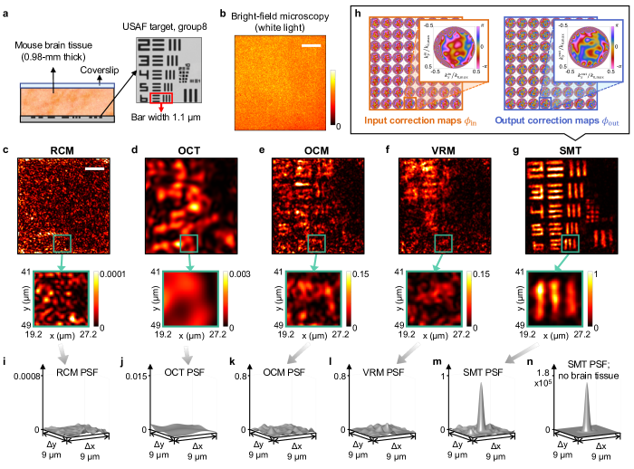
Fig. 4: Noninvasive imaging through thick tissue. a, Schematic of the sample—a USAF resolution target underneath 0.98 mm of mouse brain tissue—and a scanning electron microscope image of the USAF target before covered by the tissue. b, A standard bright-field microscope image of the sample (with white-light illumination). c–f, Reflectance confocal microscopy (RCM), optical coherence tomography (OCT), optical coherence microscopy (OCM), and volumetric reflection-matrix microscopy (VRM) images at the USAF target plane, synthesized from the measured hyperspectral reflection matrix. g, SMT image, $I_{\rm SMT}({\bf r})$, from Eqs. (2)–(3). Each pair of full view and zoom-in uses the same colorbar, and all images share the same normalization, with scales indicated on the colorbars. Scale bar in b–c: 10 µm. h, The wavefront correction phase maps for the $8\times 8$ zones in SMT. i–n, Corresponding point spread function PSF$({\bf r})$ of the sample (i–m) and of a mirror in air (n), centered at $(x_{\rm in},y_{\rm in})=(23.4,45.0)$ µm.

The SMT image resolves the 8th group of the USAF target with near perfection down to the smallest element (Fig. 4g). Here, the progression goes down to 8$\times$8 zones, with up to 22 Zernike radial orders (275 polynomial terms) in each zone (Supplementary Sect. III F). The optimized wavefront correction maps $\phi_{\rm in}({\bf k}^{\rm in}_{\parallel})$ and $\phi_{\rm out}({\bf k}^{\rm out}_{\parallel})$ are shown in Fig. 4h. Here, $\phi_{\rm out}({\bf k}_{\parallel})\neq\phi_{\rm in}(-{\bf k}_{\parallel})$ because the former includes the optical-system aberration. Notably, SMT achieves good reconstructions even when the number of frequencies or incident angles is reduced by over an order of magnitude, including when the triply-gated image only shows speckles from multiple scattering even after dispersion compensation (Supplementary Sects. V–VI).

To quantify the imaging performance, we obtain the point spread function (PSF) by evaluating Eq. (2) with a variable output position ${\bf r}={\bf r}_{\rm in}+\Delta{\bf r}$ given a fixed input position ${\bf r}_{\rm in}$ on the sixth element: ${\rm PSF}({\bf r})=I({\bf r},{\bf r}_{\rm in})$; see Supplementary Sect. VII. The PSFs of RCM, OCT, OCM, and VRM (Fig. 4i–l) have no discernible peak near $\Delta{\bf r}=0$, indicating a complete failure to image. The speckled OCM PSF averages to be 70 dB below the peak PSF of a mirror without the brain tissue (Fig. 4n), so the signal (which is buried beneath the speckled background and not visible here) has been reduced by at least ten-million-fold due to multiple scattering. The PSF of SMT (Fig. 4m) exhibits a sharp peak at $\Delta{\bf r}=0$ with 7-times the height of the tallest speckle in the background, showing we have not reached the depth limit (where the signal strength equals the background strength) of SMT yet. The SMT peak’s full width at half maximum (FWHM) is 1.08 µm, close to the mirror PSF’s 0.93 µm FWHM, demonstrating diffraction-limited resolution despite the overwhelming multiple scattering. To our knowledge, the depth-over-FWHM ratio of 910 here is the highest reported in the literature for imaging high-contrast targets inside or behind ex vivo biological tissue, which scatters about twice as much as in vivo tissue ⁶⁶.

III.2 Volumetric Imaging

We next perform 3D tomography of a dense colloid consisting of high-index titanium dioxide (TiO₂, refractive index 2.5) nanoparticles dispersed in polydimethylsiloxane (PDMS, refractive index 1.4). The nanoparticles (Sigma-Aldrich, 914320) have a typical diameter of 500 nm, and we use Mie theory to estimate the scattering and transport mean free paths to be $\ell_{\rm sca}=0.19$ mm and $\ell_{\rm tr}=0.47$ mm at $\lambda=840$ nm (Supplementary Sect. VIII). We measure the reflection matrix with a $51\times 51$ µm² field of view at one reference plane at $z_{0}=1.525$ mm depth. Using the reflection matrix, we reconstruct SMT image over a $50\times 50\times 110$ µm³ volume inside the colloid by dividing the depth of field (DOF) $\Delta z=110$ µm into 16 sub-volumes.

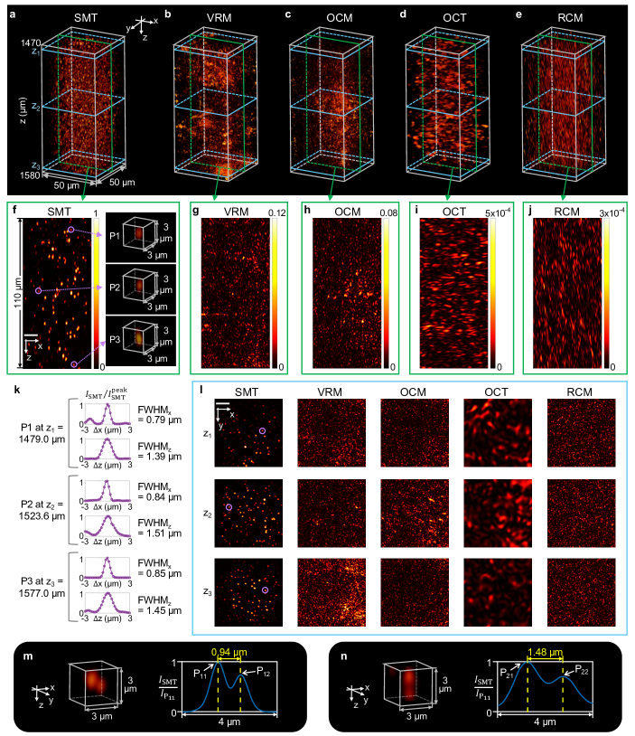
Fig. 5: Volumetric imaging inside a dense colloid. The sample consists of 500-nm-diameter TiO₂ nanoparticles dispersed in PDMS, with an estimated transport mean free path of 0.47 mm. a–e, SMT, VRM, OCM, OCT, and RCM images built from the measured hyperspectral reflection matrix. f–j, A longitudinal slice of the images at $y=23.2$ µm and close-up views of three particles at different depths in the SMT image. k, Cross sections of the three particles; $\Delta{\bf r}={\bf r}-{\bf r}_{\rm peak}$. l, Transverse slices at the depths of the three particles. m,n, SMT images of particles separated horizontally (m) and vertically (n), with center-to-center cross sections. ${\bf r}_{\rm P_{11}}=(46.39,31.29,1487.31)$ µm, ${\bf r}_{\rm P_{12}}=(46.90,31.96,1487.74)$ µm, ${\bf r}_{\rm P_{21}}=(44.04,39.12,1569.56)$ µm, and ${\bf r}_{\rm P_{22}}=(44.18,38.92,1571.02)$ µm. Scale bars in f and l: 10 µm. All images share the same normalization. Volumetric images and 2D slices use the same colorbar.

SMT creates a detailed 3D image of all the nanoparticles in this volume (Fig. 5a), with zoom-ins and cross sections of individual particles shown in Fig. 5f,k,l. A statistical analysis of these particles finds the lateral FWHM to vary from 0.7 µm to 1.0 µm within the $110$ µm DOF and the axial FWHM very close to the theoretical estimate of 1.42 µm given the spectral bandwidth of $\Delta\lambda=187$ nm here (Supplementary Sect. IX). Fig. 5m,n shows examples of SMT images of nearby particle pairs, with one pair separated horizontally by 0.94 µm and one pair separated vertically by 1.48 µm. The SMT DOF covers approximately the volume of overlap among the input/output beams in the scattering matrix measurement; it grows with the field of view and is not restricted by the Rayleigh range $z_{\rm R}$ (Supplementary Sect. IX B). Here, $z_{\rm R}=n_{\rm sam}\lambda_{0}/(\pi{\rm NA}^{2})\approx 1.5$ µm (with center wavelength $\lambda_{0}=840$ nm and $n_{\rm sam}=1.4$ for PDMS), while the SMT DOF is 73 times larger.

Like Fig. 4c–f, here we also construct VRM and synthetic OCM, OCT, and RCM images (Fig. 5b–e) for comparison, with longitudinal and transverse slices shown in Fig. 5g–j,l. For OCM and OCT, the depth of the spatial gate is fixed on one focal plane at $z_{0}=1.525$ mm when the temporal gate is scanned in $z$ (Supplementary Sect. IV B). All of these methods fail and cannot identify any of the nanoparticles at this depth. The VRM image exhibits bright artifacts at several constant-$z$ slices because its dispersion compensation maximizes the intensity at those isolated slices (Supplementary Sect. IV C).

IV Discussion

SMT provides a conceptually and mathematically simple framework that is easy to build upon. For example, besides a progression in space, one may also adopt a progression in frequency to capture the spectral variation of the optimal wavefront ^{67, 68}, a progressive increase of the NA to utilize the deeper penetration of the forward scattered photons ^{19, 20}, and/or a progressive increase of the imaging depth to reach even deeper. Global optimization can be used when the scattering is so strong that a local optimization loses its consistency. Future work may also explore other optimization schemes beyond using an image quality metric.

Validation against the ground truth is nontrivial for volumetric imaging ⁶⁹. Using the recent “augmented partial factorization” simulation method ⁷⁰, we have validated SMT through full-wave numerical simulations ⁷¹.

One can interpret RCM, OCT, and OCM as measuring the diagonal elements of the reflection matrix in a spatial basis. SMT utilizes the additional off-diagonal elements to digitally refocus to different planes (for a large DOF) and to convert the off-diagonal scattered light into focused light with wavefront corrections (for a deeper depth and a higher resolution). The price is having to measure those off-diagonal elements.

Applying wavefront-shaping methods in vivo is a challenge due to the dynamic movement of the medium ⁷². While the virtual wavefront shaping of SMT dispenses with slow SLMs, a coherent synthesis still requires measuring the matrix elements before the scatterer arrangement changes substantially. The speckle decorrelation time, primarily limited by the blood flow, is estimated as 5 ms at $\lambda=633$ nm wavelength 1 mm deep inside the mouse brain where blood is rich ⁷³ but can go beyond 30 seconds for the skull where there is less blood ⁴⁹. Currently, our total measurement time for the USAF-target-under-tissue sample is three minutes, with the majority of which spent on the mechanical acceleration and deceleration of a birefringent filter during a scan-and-stop operation of the tunable laser. Scanning the filter continuously can reduce the measurement time to 5 seconds (Supplementary Sec. I D). One can further accelerate by orders of magnitude through truncating the spatial measurement ⁵¹, parallelizing the spectral acquisition ⁷⁴, and reducing the number of frequencies or incident angles (Supplementary Sect. V–VI).

While SMT only detects contrasts in the scattering strength, digital staining and machine learning ⁷⁵ can facilitate the identification of specific structures. The phase information in $\psi_{\rm SMT}$ can help detect molecules ⁷⁶ and sub-nm displacements ^{77, 78}. One may incorporate polarization gating to select birefringent objects such as directionally oriented tissues. The hyperspectral scattering matrix can additionally resolve spectral information of the sample, such as the oxygenation of the hemoglobin. Applications that require feedback to identify the region of interest can use a subset of the matrix data to reconstruct a coarse image in real time.

Data availability: The datasets generated and analyzed during the current study are available on Zenodo ⁷⁹.

Code availability: The codes used to produce the results of the study are available on GitHub ⁸⁰.

Acknowledgments: We thank B. Applegate, S. Fraser, O. D. Miller, F. Xia, and B. Flanagan for helpful discussions. This work was supported by the Chan Zuckerberg Initiative, the National Science Foundation CAREER award (ECCS-2146021), and the University of Southern California.

Author contributions: Y.Z. and C.W.H. designed the experimental setup. Y.Z. built the setup, prepared the samples, and carried out the measurements with help from M.D. M.D. and Y.Z. developed and carried out the dispersion compensation. M.D. developed and carried out the SMT wavefront optimization with regularization and progression. Z.W. developed fast 3D reconstruction using the non-uniform fast Fourier transform. Y.Z. and Z.W. developed the index-mismatch correction. Y.Z., T.Z., and T.C. developed the control and automation of the instruments. M.D. and Y.Z. implemented the synthesis of RCM, OCT, and OCM. M.D. implemented VRM. Y.Z. performed the 3D visualization and the analyses on phase stability, sensitivity, and resolution. C.W.H. conceived the project and supervised research. C.W.H., Y.Z., and M.D. wrote the manuscript with inputs from the other coauthors. All authors discussed the results.

Competing interests: C.W.H, Z.W., Y.Z., and M.D. are inventors of US patent applications 17/972,073 and 63/472,900 titled “Multi-spectral scattering-matrix tomography” filed by the University of Southern California.

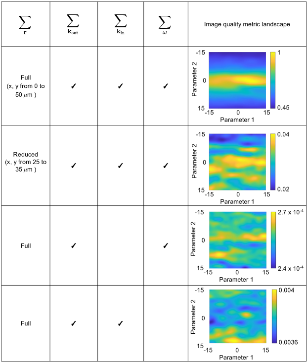
Extended Data Fig. 1: Effects of the quadruple summation on the SMT optimization landscape. The SMT optimization problem defined in Eq. (3) is high-dimensional, and here we consider two of the Zernike coefficients of $\phi_{\rm out}(\bf k_{\rm out})$ while fixing the other parameters. The right-most column plots the image quality metric $M$ of the USAF-target-under-tissue sample as a function of these two Zernike coefficients when we perform the complete quadruple summation (top row), when we reduce the range of the spatial summation ${\bf r}$ (second row), when we restrict to a single incident angle ${\bf k}_{\rm in}$ (third row), and when we restrict to a single frequency $\omega$ (bottom row) in the evaluation of $M$.

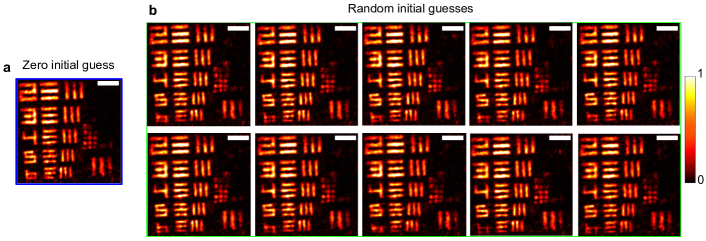
Extended Data Fig. 2: Dependence of the wavefront optimization on the initial guess. a, SMT image of the USAF-target-under-tissue sample after wavefront optimization, starting with all Zernike coefficients initialized to zero. b, SMT images after optimization, with the Zernike coefficients initialized with 10 different sets of random numbers sampled uniformly between $-0.5$ and $+0.5$ radians. Each initial guess leads to a different local optimum since the problem is nonconvex, but the image qualities of these local optima are comparable. All images adopt the same regularization and progression strategies. Scale bar: 10 µm.

References

- [1] Yoon, S. et al. Deep optical imaging within complex scattering media. Nat. Rev. Phys 2, 141–158 (2020).
- [2] Bertolotti, J. & Katz, O. Imaging in complex media. Nat. Phys. 18, 1008–1017 (2022).
- [3] Calzavara-Pinton, P., Longo, C., Venturini, M., Sala, R. & Pellacani, G. Reflectance confocal microscopy for in vivo skin imaging. Photochem. Photobiol. 84, 1421–1430 (2008).
- [4] Xia, F. et al. In vivo label-free confocal imaging of the deep mouse brain with long-wavelength illumination. Biomed. Opt. Express 9, 6545–6555 (2018).
- [5] Fercher, A. F., Drexler, W., Hitzenberger, C. K. & Lasser, T. Optical coherence tomography—principles and applications. Rep. Prog. Phys. 66, 239 (2003).
- [6] Aguirre, A. D., Zhou, C., Lee, H.-C., Ahsen, O. O. & Fujimoto, J. G. Optical coherence microscopy. In Drexler, W. & Fujimoto, J. G. (eds.) Optical Coherence Tomography: Technology and Applications, chap. 28, 865–911 (Springer, Cham, 2015).
- [7] Ralston, T. S., Marks, D. L., Scott Carney, P. & Boppart, S. A. Interferometric synthetic aperture microscopy. Nat. Phys. 3, 129–134 (2007).
- [8] Hampson, K. M. et al. Adaptive optics for high-resolution imaging. Nat. Rev. Methods Primers 1, 68 (2021).
- [9] Tippie, A. E., Kumar, A. & Fienup, J. R. High-resolution synthetic-aperture digital holography with digital phase and pupil correction. Opt. Express 19, 12027–12038 (2011).
- [10] Adie, S. G., Graf, B. W., Ahmad, A., Carney, P. S. & Boppart, S. A. Computational adaptive optics for broadband optical interferometric tomography of biological tissue. Proc. Natl. Acad. Sci. U.S.A. 109, 7175–7180 (2012).
- [11] Hillmann, D. et al. Aberration-free volumetric high-speed imaging of in vivo retina. Sci. Rep. 6, 35209 (2016).
- [12] Horton, N. G. et al. In vivo three-photon microscopy of subcortical structures within an intact mouse brain. Nat. Photon. 7, 205–209 (2013).
- [13] Streich, L. et al. High-resolution structural and functional deep brain imaging using adaptive optics three-photon microscopy. Nat. Methods 18, 1253–1258 (2021).
- [14] Jin, D., Zhou, R., Yaqoob, Z. & So, P. T. Tomographic phase microscopy: principles and applications in bioimaging. J. Opt. Soc. Am. B 34, B64–B77 (2017).
- [15] Park, Y., Depeursinge, C. & Popescu, G. Quantitative phase imaging in biomedicine. Nat. Photon. 12, 578–589 (2018).
- [16] Tahir, W., Kamilov, U. S. & Tian, L. Holographic particle localization under multiple scattering. Adv. Photonics 1, 036003 (2019).
- [17] Lim, J., Ayoub, A. B., Antoine, E. E. & Psaltis, D. High-fidelity optical diffraction tomography of multiple scattering samples. Light Sci. Appl. 8, 82 (2019).
- [18] Chen, M., Ren, D., Liu, H.-Y., Chowdhury, S. & Waller, L. Multi-layer born multiple-scattering model for 3D phase microscopy. Optica 7, 394–403 (2020).
- [19] Zhao, Y. et al. Dual-axis optical coherence tomography for deep tissue imaging. Opt. Lett. 42, 2302–2305 (2017).
- [20] Cua, M., Blochet, B. & Yang, C. Speckle-resolved optical coherence tomography for mesoscopic imaging within scattering media. Biomed. Opt. Express 13, 2068–2081 (2022).
- [21] Wang, L. V. & Hu, S. Photoacoustic tomography: in vivo imaging from organelles to organs. Science 335, 1458–1462 (2012).
- [22] Pian, Q. et al. Multimodal biomedical optical imaging review: towards comprehensive investigation of biological tissues. Curr. Mol. Imaging 3, 72–87 (2014).
- [23] Lal, C. & Leahy, M. J. An updated review of methods and advancements in microvascular blood flow imaging. Microcirculation 23, 345–363 (2016).
- [24] Rotter, S. & Gigan, S. Light fields in complex media: Mesoscopic scattering meets wave control. Rev. Mod. Phys. 89, 015005 (2017).
- [25] Cao, H., Mosk, A. P. & Rotter, S. Shaping the propagation of light in complex media. Nat. Phys. 18, 994–1007 (2022).
- [26] Horstmeyer, R., Ruan, H. & Yang, C. Guidestar-assisted wavefront-shaping methods for focusing light into biological tissue. Nat. Photon. 9, 563–571 (2015).
- [27] Vellekoop, I. M. & Mosk, A. Focusing coherent light through opaque strongly scattering media. Opt. Lett. 32, 2309–2311 (2007).
- [28] Popoff, S., Lerosey, G., Fink, M., Boccara, A. C. & Gigan, S. Image transmission through an opaque material. Nat. Commun. 1, 81 (2010).
- [29] Yaqoob, Z., Psaltis, D., Feld, M. S. & Yang, C. Optical phase conjugation for turbidity suppression in biological samples. Nat. Photon. 2, 110–115 (2008).
- [30] Cheng, Z., Li, C., Khadira, A., Zhang, Y. & Wang, L. V. High-gain and high-speed wavefront shaping through scattering media. Nat. Photon. (2023).
- [31] Tang, J., Germain, R. N. & Cui, M. Superpenetration optical microscopy by iterative multiphoton adaptive compensation technique. Proc. Natl. Acad. Sci. U.S.A. 109, 8434–8439 (2012).
- [32] Papadopoulos, I. N., Jouhanneau, J.-S., Poulet, J. F. & Judkewitz, B. Scattering compensation by focus scanning holographic aberration probing (F-SHARP). Nat. Photon. 11, 116–123 (2017).
- [33] Aizik, D. & Levin, A. Non-invasive and noise-robust light focusing using confocal wavefront shaping. Preprint at https://arxiv.org/abs/2301.11421 (2023).
- [34] Xu, X., Liu, H. & Wang, L. V. Time-reversed ultrasonically encoded optical focusing into scattering media. Nat. Photon. 5, 154–157 (2011).
- [35] Wang, Y. M., Judkewitz, B., DiMarzio, C. A. & Yang, C. Deep-tissue focal fluorescence imaging with digitally time-reversed ultrasound-encoded light. Nat. Commun. 3, 928 (2012).
- [36] Ma, C., Xu, X., Liu, Y. & Wang, L. V. Time-reversed adapted-perturbation (TRAP) optical focusing onto dynamic objects inside scattering media. Nat. Photon. 8, 931–936 (2014).
- [37] Zhou, E. H., Ruan, H., Yang, C. & Judkewitz, B. Focusing on moving targets through scattering samples. Optica 1, 227–232 (2014).
- [38] Judkewitz, B., Horstmeyer, R., Vellekoop, I. M., Papadopoulos, I. N. & Yang, C. Translation correlations in anisotropically scattering media. Nat. Phys. 11, 684–689 (2015).
- [39] Osnabrugge, G., Horstmeyer, R., Papadopoulos, I. N., Judkewitz, B. & Vellekoop, I. M. Generalized optical memory effect. Optica 4, 886–892 (2017).
- [40] Bertolotti, J. et al. Non-invasive imaging through opaque scattering layers. Nature 491, 232–234 (2012).
- [41] Katz, O., Heidmann, P., Fink, M. & Gigan, S. Non-invasive single-shot imaging through scattering layers and around corners via speckle correlations. Nat. Photon. 8, 784–790 (2014).
- [42] Yeminy, T. & Katz, O. Guidestar-free image-guided wavefront shaping. Sci. Adv. 7, eabf5364 (2021).
- [43] Feng, B. Y. et al. NeuWS: Neural wavefront shaping for guidestar-free imaging through static and dynamic scattering media. Sci. Adv. 9, eadg4671 (2023).
- [44] Kang, S. et al. Imaging deep within a scattering medium using collective accumulation of single-scattered waves. Nat. Photon. 9, 253–258 (2015).
- [45] Badon, A. et al. Smart optical coherence tomography for ultra-deep imaging through highly scattering media. Sci. Adv. 2, e1600370 (2016).
- [46] Badon, A. et al. Distortion matrix concept for deep optical imaging in scattering media. Sci. Adv. 6, eaay7170 (2020).
- [47] Kang, S. et al. High-resolution adaptive optical imaging within thick scattering media using closed-loop accumulation of single scattering. Nat. Commun. 8, 2157 (2017).
- [48] Yoon, S., Lee, H., Hong, J. H., Lim, Y.-S. & Choi, W. Laser scanning reflection-matrix microscopy for aberration-free imaging through intact mouse skull. Nat. Commun. 11, 5721 (2020).
- [49] Kwon, Y. et al. Computational conjugate adaptive optics microscopy for longitudinal through-skull imaging of cortical myelin. Nat. Commun. 14, 105 (2023).
- [50] Li, B. et al. Efficient framework of solving time-gated reflection matrix for imaging through turbid medium. Opt. Express 31, 15461–15473 (2023).
- [51] Najar, U. et al. Non-invasive retrieval of the time-gated transmission matrix for optical imaging deep inside a multiple scattering medium. Preprint at https://arxiv.org/abs/2303.06119 (2023).
- [52] Lee, Y.-R., Kim, D.-Y., Jo, Y., Kim, M. & Choi, W. Exploiting volumetric wave correlation for enhanced depth imaging in scattering medium. Nat. Commun. 14, 1878 (2023).
- [53] Popoff, S. M. et al. Measuring the transmission matrix in optics: an approach to the study and control of light propagation in disordered media. Phys. Rev. Lett. 104, 100601 (2010).
- [54] Mounaix, M. et al. Spatiotemporal coherent control of light through a multiple scattering medium with the multispectral transmission matrix. Phys. Rev. Lett. 116, 253901 (2016).
- [55] De Boer, J. F., Leitgeb, R. & Wojtkowski, M. Twenty-five years of optical coherence tomography: the paradigm shift in sensitivity and speed provided by Fourier domain OCT. Biomed. Opt. Express 8, 3248–3280 (2017).
- [56] Bender, N. et al. Coherent enhancement of optical remission in diffusive media. Proc. Natl. Acad. Sci. U.S.A. 119, e2207089119 (2022).
- [57] Barnett, A. H., Magland, J. & af Klinteberg, L. A parallel nonuniform fast Fourier transform library based on an “exponential of semicircle” kernel. SIAM J. Sci. Comput. 41, C479–C504 (2019).
- [58] Wolf, E. Three-dimensional structure determination of semi-transparent objects from holographic data. Opt. Commun. 1, 153–156 (1969).
- [59] Hell, S., Reiner, G., Cremer, C. & Stelzer, E. H. Aberrations in confocal fluorescence microscopy induced by mismatches in refractive index. J. Microsc. 169, 391–405 (1993).
- [60] Liu, D. C. & Nocedal, J. On the limited memory BFGS method for large scale optimization. Math. Program. 45, 503–528 (1989).
- [61] Johnson, S. G. The NLopt nonlinear-optimization package. http://github.com/stevengj/nlopt.
- [62] Wojtkowski, M. et al. Ultrahigh-resolution, high-speed, Fourier domain optical coherence tomography and methods for dispersion compensation. Opt. Express 12, 2404–2422 (2004).
- [63] Noll, R. J. Zernike polynomials and atmospheric turbulence. J. Opt. Soc. Am. 66, 207–211 (1976).
- [64] Verrier, N. & Atlan, M. Off-axis digital hologram reconstruction: some practical considerations. Appl. Opt. 50, H136–H146 (2011).
- [65] Xiong, W., Hsu, C. W. & Cao, H. Long-range spatio-temporal correlations in multimode fibers for pulse delivery. Nat. Commun. 10, 2973 (2019).
- [66] Kobat, D. et al. Deep tissue multiphoton microscopy using longer wavelength excitation. Opt. Express 17, 13354–13364 (2009).
- [67] Van Beijnum, F., Van Putten, E. G., Lagendijk, A. & Mosk, A. P. Frequency bandwidth of light focused through turbid media. Opt. Lett. 36, 373–375 (2011).
- [68] Hsu, C. W., Goetschy, A., Bromberg, Y., Stone, A. D. & Cao, H. Broadband coherent enhancement of transmission and absorption in disordered media. Phys. Rev. Lett. 115, 223901 (2015).
- [69] Krauze, W. et al. 3D scattering microphantom sample to assess quantitative accuracy in tomographic phase microscopy techniques. Sci. Rep. 12, 19586 (2022).
- [70] Lin, H.-C., Wang, Z. & Hsu, C. W. Fast multi-source nanophotonic simulations using augmented partial factorization. Nat. Comput. Sci 2, 815–822 (2022).
- [71] Wang, Z., Zhang, Y. & Hsu, C. W. Full-wave simulations of tomographic optical imaging inside scattering media. Preprint at https://arxiv.org/abs/2308.07244 (2023).
- [72] Liu, Y., Ma, C., Shen, Y., Shi, J. & Wang, L. V. Focusing light inside dynamic scattering media with millisecond digital optical phase conjugation. Optica 4, 280–288 (2017).
- [73] Qureshi, M. M. et al. In vivo study of optical speckle decorrelation time across depths in the mouse brain. Biomed. Opt. Express 8, 4855–4864 (2017).
- [74] Gao, L. & Smith, R. T. Optical hyperspectral imaging in microscopy and spectroscopy – a review of data acquisition. J. Biophotonics 8, 441–456 (2015).
- [75] Rivenson, Y. et al. PhaseStain: the digital staining of label-free quantitative phase microscopy images using deep learning. Light Sci. Appl. 8, 23 (2019).
- [76] Taylor, R. W. & Sandoghdar, V. Interferometric scattering microscopy: Seeing single nanoparticles and molecules via rayleigh scattering. Nano Lett. 19, 4827–4835 (2019).
- [77] Akkin, T., Davé, D. P., Milner, T. E. & Rylander III, H. G. Detection of neural activity using phase-sensitive optical low-coherence reflectometry. Opt. Express 12, 2377–2386 (2004).
- [78] Kim, W., Kim, S., Huang, S., Oghalai, J. S. & Applegate, B. E. Picometer scale vibrometry in the human middle ear using a surgical microscope based optical coherence tomography and vibrometry system. Biomed. Opt. Express 10, 4395–4410 (2019).
- [79] https://doi.org/10.5281/zenodo.8231064.
- [80] https://github.com/complexphoton/SMTexperiment.