The coherent structure of the energy cascade in isotropic turbulence

Abstract

The energy cascade, i.e. the transfer of kinetic energy from large-scale to small-scale flow motions, has been the cornerstone of turbulence theories and models since the 1940s. However, understanding the spatial organization of the energy transfer has remained elusive. In this work, we answer the question: What are the characteristic flow patterns surrounding regions of intense energy transfer? To that end, we utilize numerical data of isotropic turbulence to investigate the three-dimensional spatial structure of the energy cascade in the inertial range. Our findings indicate that forward energy-transfer events are predominantly confined in the high strain-rate region created between two distinct zones of elevated enstrophy. On average, these zones manifest in the form of two hairpin-like shapes with opposing orientations. The mean velocity field associated with the energy transfer exhibits a saddle point topology when observed in the frame of reference local to the event. The analysis also shows that the primary driving mechanism for the cascade involves strain-rate self-amplification, which is responsible for 85% of the energy transfer, whereas vortex stretching accounts for less than 15%.

1 Introduction

Turbulence exhibits a wide range of flow scales, whose non-linear interactions still challenge our intellectual ability to understand even the simplest flows. These interactions are responsible for the cascading of kinetic energy from large eddies to the smallest eddies, where the energy is finally dissipated (e.g. Richardson, 1922; Obukhov, 1941; Kolmogorov, 1941). Given the ubiquity of turbulence, a deeper understanding of the energy transfer among flow scales would enable significant progress to be made across various fields ranging from combustion (e.g. Veynante & Vervisch, 2002), meteorology (e.g. Bodenschatz, 2015), and astrophysics (e.g. Young & Read, 2017) to engineering applications of external aerodynamics and hydrodynamics (e.g. Sirovich & Karlsson, 1997; Hof et al., 2010; Marusic et al., 2010; Kühnen et al., 2018).

The phenomenological description of the turbulent cascade in terms of interactions among eddies at different scales was first proposed by Richardson (1920) and later by Obukhov (1941). Since then, substantial efforts have been directed toward the characterization of inter-scale kinetic energy transfer. The statistical description of the transfer of energy from large to small scales was introduced in the classical paper by Kolmogorov (1941). Since then, a large body of research has been devoted to addressing two outstanding questions about the energy cascade: 1) Is the transfer of kinetic energy from large to small scales local in scale? and 2) What are the physical mechanisms driving the transfer of energy among scales? Here, we pose a third question: 3) What are the characteristic flow patterns surrounding regions of intense energy transfer? The three questions above are interconnected, and we anticipate that addressing question 3) will also shed light on question 2).

There is general agreement from the community that the answer to the first question is yes. The net transfer of energy from large to small scales is mainly accomplished by interactions among flow motions of similar size. The conclusion is supported by evidence from diverse approaches, such as scaling analysis (Zhou, 1993a, b; Eyink, 1995; Aoyama et al., 2005; Eyink, 2005; Mininni et al., 2006, 2008; Aluie & Eyink, 2009; Eyink & Aluie, 2009), triadic interactions in Fourier space (Domaradzki & Rogallo, 1990; Domaradzki et al., 2009), time correlations (Cardesa et al., 2015, 2017), and information-theoretic causality (Lozano-Durán & Arranz, 2022), to name a few.

The degree of consensus is lower regarding the second question. Several theories have been proposed to describe the physical mechanism(s) that enable the transfer of energy from larger to smaller scales throughout the inertial range. One of the first mechanisms proposed is based on the concept of vortex stretching. In this scenario, vorticity is stretched by the strain-rate either at the same scale or at a larger scale (Taylor & Green, 1937; Taylor, 1938; Tennekes et al., 1972; Davidson et al., 2008; Hamlington et al., 2008; Leung et al., 2012; Lozano-Durán et al., 2016; Doan et al., 2018). Some authors have further proposed that the mechanistic details of the process can be explained by successive reconnections of anti-parallel vortex tubes (Melander & Hussain, 1988; Hussain & Duraisamy, 2011; Goto et al., 2017; Yao & Hussain, 2020), vortex reconnection of two long, straight anti-parallel vortex tubes with localized bumps (Kerr, 2013), and the presence of helictical instabilities in characteristic of vortex rings (Brenner et al., 2016; McKeown et al., 2018). These viewpoints, while not dynamically equivalent, are still compatible with the vortex-stretching driven energy cascade.

The main competing theory to the vortex stretching mechanism is the self-amplification of the rate-of-strain either by same-scale interactions or by the amplification from larger scale strain-rate (e.g. Tsinober, 2009; Paul et al., 2017; Sagaut & Cambon, 2008; Carbone & Bragg, 2020; Vela-Martín & Jiménez, 2021). In both scenarios, the strain-rate self-amplification stands as the key contributor to the transfer of energy among scales, whereas vortex stretching is merely the effect (rather than the cause) of the energy cascade. Given the kinematic relationship between vortex stretching and strain-rate self-amplification (Betchov, 1956; Capocci et al., 2023), some authors have argued that both mechanisms play a relevant role in the dynamics of the energy cascade (Johnson, 2020, 2021).

The studies above have helped advance our understanding of the physics of the energy cascade; however, less is known about flow patterns associated with the cascading process. With the advent of novel flow identification techniques (e.g. del Álamo et al., 2004; Lozano-Durán et al., 2012; Lozano-Durán & Jiménez, 2014; Dong et al., 2017, 2020), the three-dimensional characterization of turbulent structures is now achievable to complete the picture. In this work, we shed light on the characteristic flow patterns associated with the energy cascade by investigating the spatial three-dimensional structure of the flow conditioned to intense energy transfer events.

The work is organized as follows. The method is presented in §2, where we introduce the numerical dataset, filtering procedure, structure identification and characterization, and conditional flow field methodology. The results concerning the dominant flow patterns associated with the energy transfer are discussed in §3 and conclusions are offered in §4.

2 Methods

2.1 Numerical dataset and filtering procedure

We use direct numerical simulations of isotropic turbulence from Cardesa et al. (2015). The numerical setup corresponds to isotropically forced turbulence within a triply periodic domain at $\mathrm{Re}_{\lambda}=146,236$, and $384$, where $\mathrm{Re}_{\lambda}$ is the Reynolds number based on the Taylor microscale. The simulations are labeled as HIT1 (for $\mathrm{Re}_{\lambda}=146$), HIT2 (for $\mathrm{Re}_{\lambda}=236$), and HIT3 (for $\mathrm{Re}_{\lambda}=384$). Table 1 contains the numerical details of the simulations in terms of grid resolution, domain size, and number of snapshots. The reader is referred to Cardesa et al. (2015) for additional information about the numerical setup.

Case	$\mathrm{Re}_{\lambda}$	$N_{x}\times N_{y}\times N_{z}$	$\left(L_{x}\times L_{y}\times L_{z}\right)/\eta$	$L_{o}/\eta$	$N_{t}$	$\Delta/\eta$	$\Delta t/T_{o}$
HIT1	$146$	$256^{3}$	$506^{3}$	$425$	30	2	5.5
HIT2	$236$	$512^{3}$	$1011^{3}$	$876$	48	2	0.33
HIT3	$384$	$1024^{3}$	$2022^{3}$	$1813$	30	2	0.13

Table 1: Summary of the main parameters of the simulations. $\mathrm{Re}_{\lambda}$ is the Reynolds number based on the Taylor microscale. $N_{i}$ and $L_{i}$ are the number of spatial Fourier modes and the domain size in the directions $i=x,y,z$. The Kolmogorov and integral length scales are $\eta=\left(\nu^{3}/\bar{\varepsilon}\right)^{1/4}$ and $L_{o}=\bar{K}^{3/2}/\bar{\varepsilon}$, respectively, where $\bar{K}$ and $\bar{\epsilon}$ are the space-time averaged turbulent kinetic energy and dissipation. The times are normalized by $T_{o}=\bar{K}/\bar{\varepsilon}$ and $N_{t}$ is the number of instantaneous flow fields used to collect statistics; $\Delta/\eta$ is the grid resolution and $\Delta t/T_{o}$ is the time interval between instantaneous flow fields used for the analysis.

To investigate the structure of the energy transfer, the velocity field is decomposed into large and small scales using a low-pass Gaussian filter such that $u_{i}=\widetilde{u}_{i}+u^{\prime}_{i}$ for $i=1,2,3$, where ${u}_{i}$ represents the $i$-th component of the instantaneous velocity, $\widetilde{u}_{i}$ is the filtered velocity, and $u^{\prime}_{i}$ corresponds to the remaining fluctuating velocity component. The filter is isotropic and given in Fourier space by the Gaussian kernel $\hat{G}(\mathbf{\kappa})=\exp[-(r\kappa)^{2}/24]$, where $\kappa=\boldsymbol{|\kappa|}$ is the magnitude of the wavenumber vector ($\boldsymbol{\kappa}$), and $r$ is the filter width. Four filter widths are investigated: $r/\eta=20,30,40,$ and $60$, where $\eta=\left(\nu^{3}/\bar{\varepsilon}\right)^{1/4}$ is the Kolmogorov length-scale, $\nu$ is the kinematic viscosity, and $\bar{\epsilon}$ is the space-time averaged dissipation of turbulent kinetic energy. Figure 1 compares one instant of the unfiltered velocity and the filtered velocity for $r=30\eta$. The values of $r$ were chosen to span across the inertial range of the turbulence cascade (Cardesa et al., 2015). The kinetic energy spectra $E(\kappa)$ for the three Reynolds numbers are shown in figure 2(a). As expected, the viscous and inertial range of $E(\kappa)$ collapse in Kolmogorov units, defined by $\eta$ and the Kolmogorov velocity-scale $u_{\eta}=(\nu\bar{\epsilon})^{1/4}$. The compensated kinetic energy spectra $\kappa^{5/3}E(\kappa)$ for HIT3 is included in figure 2(b) for the unfiltered case and for $r/\eta=20,30,40$ and $60$. The latter shows that the filtered widths lie within the inertial range of the moderate Reynolds numbers considered.

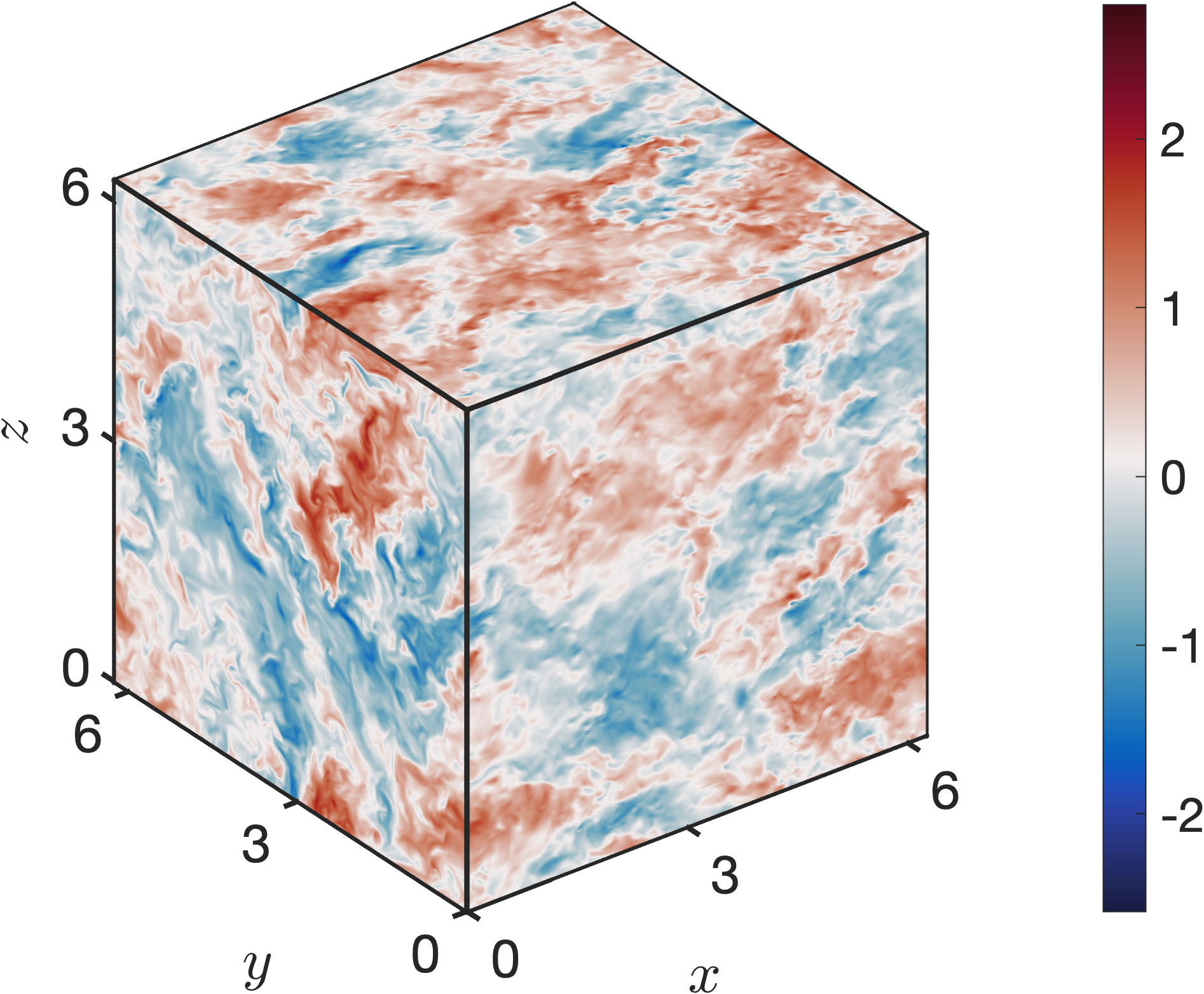
(a)

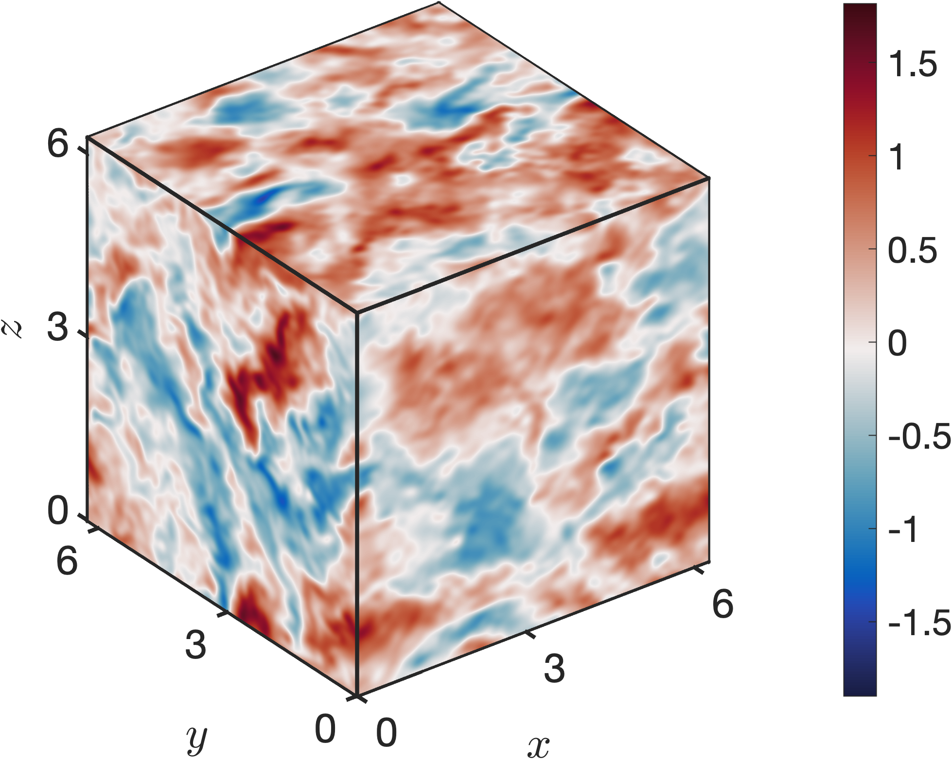
(b)

Figure 1: Instantaneous velocity field for (a) $u_{1}$ (unfiltered) and (b) $\widetilde{u}_{1}$ (filtered) for $r=30\eta$. The velocity is normalized by $\sqrt{\langle u_{i}u_{i}\rangle}$ in panel (a) and by $\sqrt{\langle\tilde{u}_{i}\tilde{u}_{i}}\rangle$ in panel (b), where $\langle\cdot\rangle$ denotes average over homogeneous directions and time.

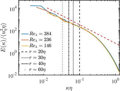
(a)

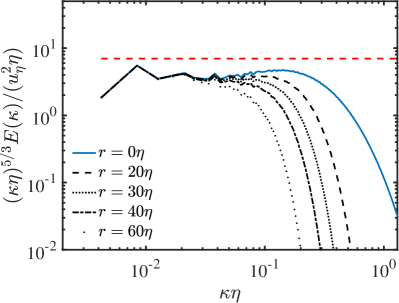
(b)

Figure 2: The kinetic energy spectra $E(\kappa)$ as a function of the wavenumber $\kappa$. The spectra and wavenumbers are normalized with the Kolmogorov length-scale $\eta$ and the Kolmogorov velocity-scale $u_{\eta}$. (a) $E(\kappa)$ for the unfiltered velocity. The vertical lines correspond to the different filter widths. (b) Compensated kinetic energy spectra $\kappa^{5/3}E(\kappa)$ for different filtered widths and for case HIT3. The red dashed line in both panels is $E(k)\sim k^{-5/3}$.

2.2 Identification of intense energy transfer events

The kinetic energy equation for the filtered velocity field is

$$\frac{D}{Dt}\left(\frac{1}{2}\widetilde{u}_{i}\widetilde{u}_{i}\right)=-\frac{\partial}{\partial x_{j}}\left(\widetilde{u_{j}}\widetilde{p}+\widetilde{u}_{i}\tau_{ij}-2\nu\widetilde{u}_{i}\widetilde{S}_{ij}\right)-2\nu\widetilde{S}_{ij}\widetilde{S}_{ij}-\Pi+\widetilde{u}_{i}{\widetilde{f_{i}}},$$ (1)

where repeated indices imply summation, ${D}/{Dt}={\partial}/{\partial t}+\widetilde{u}_{j}{\partial}/{\partial x_{j}}$ is the material derivative, $\widetilde{S}_{ij}=\left(\partial\widetilde{u}_{i}/\partial x_{j}+\partial\widetilde{u}_{j}/\partial x_{i}\right)/2$ is the strain-rate tensor for the filtered velocity, and $\widetilde{f_{i}}$ is the forcing term. The first and second terms on the right-hand side of Eq. (1) represent the spatial flux of the kinetic energy and dissipation of the energy, respectively. The term $\Pi=-\tau_{ij}\widetilde{S}_{ij}$ with $\tau_{ij}=\widetilde{u_{i}u_{j}}-\widetilde{u}_{i}\widetilde{u}_{j}$ is the inter-scale kinetic energy transfer, which is the quantity of interest here. A positive value of $\Pi$ signifies the transfer of kinetic energy from scales above the filter cut-off to smaller scales (forward cascade). Conversely, a negative value of $\Pi$ indicates the transfer of kinetic energy from sub-filtered flow motions to scales above the filter cut-off (backward cascade). It is worth noting that alternative definitions of $\Pi$ are possible by rearranging the terms within the spatial flux in Eq. (1), and other options have been proposed in the literature (e.g., Vela-Martín, 2022; Cardesa & Lozano-Durán, 2019). Here, we adopt $\Pi=-\tau_{ij}\widetilde{S}_{ij}$, which is one of the most widely accepted and studied definitions within the community.

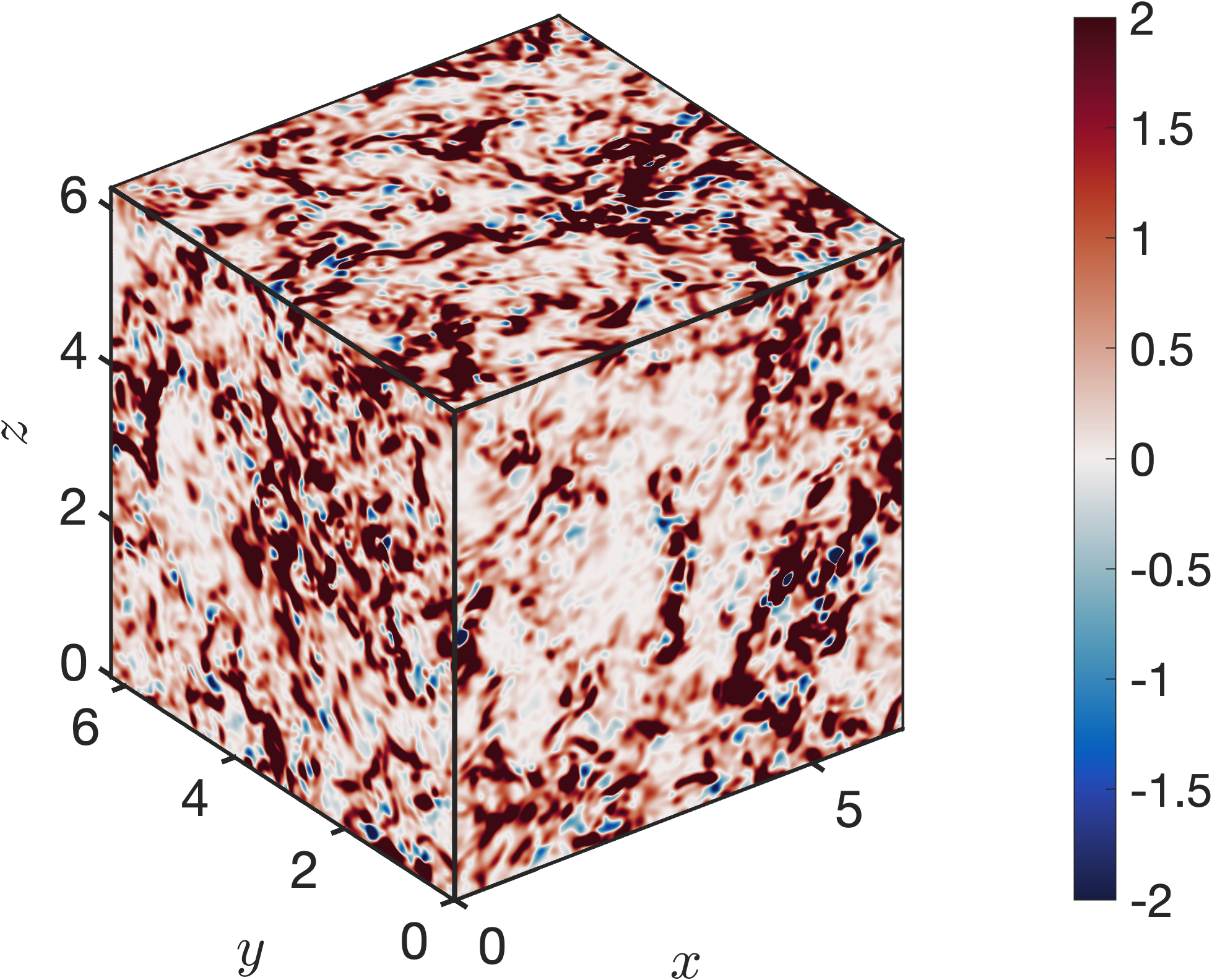
(a)

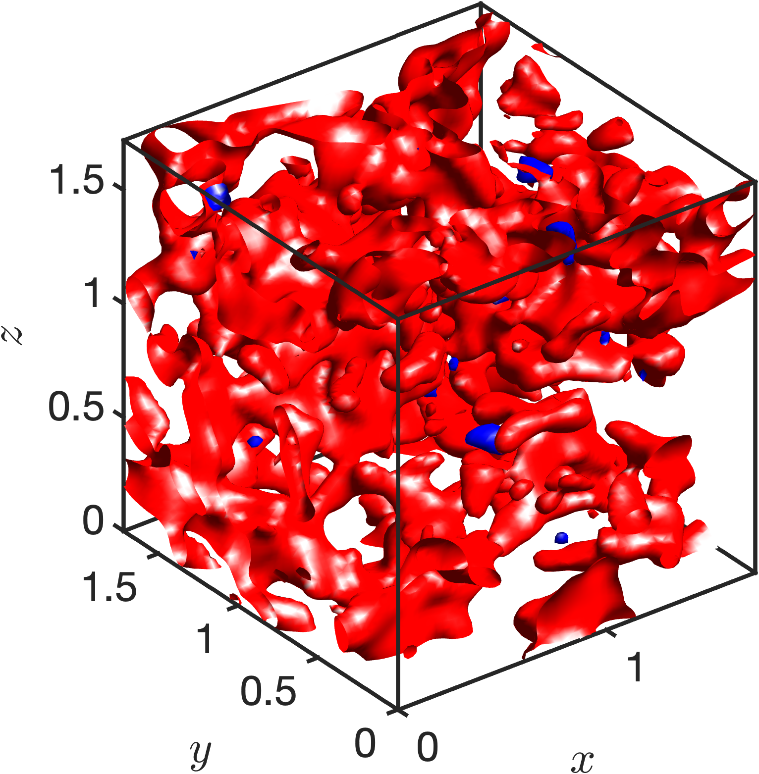
(b)

Figure 3: Instantaneous inter-scale kinetic energy transfer. (a) $\Pi$ and (b) regions with $\Pi>\Pi_{\text{rms}}$ (red) and $\Pi<-\Pi_{\text{rms}}$ (blue). The results are for case HIT2 and $r=30\eta$.

The instantaneous inter-scale kinetic energy transfer at one instance is visualized in figure 3(a). Our primary efforts are directed toward analyzing the coherent structure of the flow in the vicinity of intense forward cascade events. Regions of strong positive $\Pi$ are isolated by thresholding the field with the parameter $\alpha>0$, such that $\Pi>\alpha\Pi_{\text{rms}}$, where $\Pi_{\text{rms}}$ represents the standard deviation of $\Pi$ over all the dataset. The value of $\alpha=1$ is selected following the work of Dong et al. (2020). Appendix §A shows that the conclusions drawn in this manuscript also hold for other values of $\alpha$. Then, individual three-dimensional $\Pi$-structures are defined as contiguous regions in space satisfying $\Pi>\Pi_{\text{rms}}$. These structures will be utilized as markers to conditionally average the flow around them. The $\Pi$-structures occupy less than 20% of the total fluid volume but contribute to 70% of the total kinetic energy transfer. Figure 3(b) visualizes the regions associated with forward (red, $\Pi>\Pi_{\text{rms}}$) and backward (blue, $\Pi<-\Pi_{\text{rms}}$) intense cascade events for a given snapshot. Forward cascade events dominate over their backward counterparts, as clearly appreciated in figure 3(b), consistent with previous results in the literature (e.g. Piomelli et al., 1991; Borue & Orszag, 1998; Cerutti & Meneveau, 1998). We will focus solely on the forward energy cascade, while we do not address inverse cascading events. This decision is primarily driven by two factors. Firstly, the number of intense backward cascade events is orders of magnitude smaller than the forward events, as illustrated in figure 3(b). Secondly, whereas the importance of the forward energy cascade is widely recognized in terms of dynamics and reduced-order modeling of the flow, the same consensus is not established for the inverse energy cascade in three-dimensional turbulence. Recent works have suggested that the inverse energy cascade may play a minor role in the flow dynamics or even lack physical significance (e.g., Vela-Martín & Jiménez, 2021; Vela-Martín, 2022; Lozano-Durán & Arranz, 2022).

2.3 Geometric properties of $\Pi$-structures

We characterize the geometric properties of the $\Pi$-structures in terms of size and fractal dimensions across different filter widths and Reynolds numbers. The three typical lengths of each $\Pi$-structure, $l_{x}\geq l_{y}\geq l_{z}$, are measured by the edges of their bounding boxes. A local frame of reference is calculated using the principal axes of inertia of each $\Pi$-structure, which determines the orientation of the bounding boxes. Examples of the bounding boxes and the circumscribed $\Pi$-structures are illustrated in figure 5. The joint probability density function (JPDF) of $l_{x}/\eta$ and $l_{y}/\eta$ is shown in figure 4(a) for different filter widths at Re${}_{\lambda}=384$. The lengths follow a self-similar trend along $l_{x}\sim l_{y}$, i.e., longer structures tend to be proportionally wider. Although not shown, the same self-similar relationship holds for the third length, $l_{x}\sim l_{z}$. Figure 4(a) shows that, as expected, the lengths of the structures become larger with increasing values of $r$ and that these lengths also follow the self-similar relation $l_{x}\sim l_{y}$. The aspect ratios of the bounding boxes are quantified in figure 4(b), which features the JPDF of $l_{y}/l_{x}$ and $l_{z}/l_{x}$ for different values of $r$ at Re${}_{\lambda}=384$. The results reveals that aspect ratios are similarly distributed across scales, with values centered around $l_{y}/l_{x}\approx 0.6$ and $l_{z}/l_{x}\approx 0.3$. Analogous aspect ratio relationships are obtained across the three Reynolds numbers considered (figure 4d).

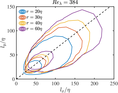
(a)

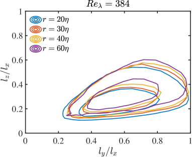
(b)

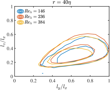
(c)

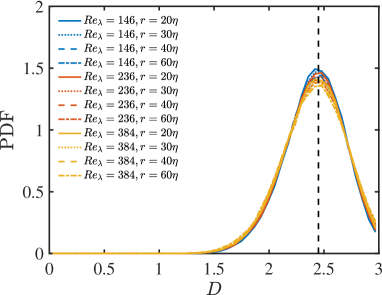
(d)

Figure 4: (a) Joint probability density function of the sizes $l_{x}$ and $l_{y}$ of the $\Pi$-structures for different filter widths. The dashed line is $l_{y}=l_{x}/1.6$. (b,c) Joint probability density function of the aspect ratios $l_{y}/l_{x}$ and $l_{z}/l_{x}$ for (b) different filter widths for HIT3 and (c) different Re_λ for $r=40\eta$. (d) Probability density function of the fractal dimension $D$ of the $\Pi$-structures for different filter widths and Reynolds numbers. The vertical dashed line is $D=2.45$.

The typical shape of the $\Pi$-structures is quantified via their fractal dimension. We employed the box-counting method to calculate the Minkowski-Bouligand dimension of each $\Pi$-structure (Falconer, 2004; Moisy & Jiménez, 2004). For each object, the computational domain is divided into cubes with a side length of $l$, and the number $N_{b}(l)$ of boxes containing at least one point of the object is counted. In the case of a pure fractal set with dimension $D$, the number of boxes would follow a power law $N_{b}(l)\sim l^{-D}$. In practice, this relationship only holds within a restricted range of scales, bounded by a large-scale and a small-scale cutoff. We define the local fractal dimension as

$$D_{l}(l)=-\frac{\mathrm{d}\ln N_{b}(l)}{\mathrm{d}\ln l}.$$ (2)

The fractal dimension of the object can be taken along the range over which the slope of $D_{l}(l)$ is approximately constant.

Figure 4(d) shows the PDF of the fractal dimensions for the $\Pi$-structures for different filter widths and Re_λ. Space-filling spheroidal shapes would exhibit fractal dimensions close to $D\approx 3$, whereas sheet-like or filament-like structures would have $D\approx 2$ or $D\approx 1$, respectively. The PDF of $D$ reveals a bell-shaped distribution centered around $2.45$, suggesting that the objects have an intermediate form between sheet-like and strictly spheroidal shapes. Therefore, although some $\Pi$-structures may exhibit complex shapes, most often they resemble elongated ellipsoids with arbitrary orientation. In summary, the results from this section show that $\Pi$-structures are geometrically self-similar across scales within the inertial range and for the three Re_λ considered. This finding provides justification for the conditional averaging procedure introduced in the subsequent section.

2.4 Conditional-averaged flow fields

We calculate the average flow surrounding $\Pi$-structures accounting for symmetries and self-similarity. Figure 5 presents a schematic of the conditional averaging procedure. This process involves three steps, illustrated in the figure from left to right: identification of the $\Pi$-structures, calculation of the local frame of reference, and computation of the conditional-averaged flow field. Each step is detailed below.

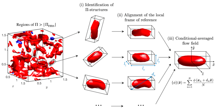
Figure 5: Schematic of the conditional averaging procedure. The normalized directions of the local frame of reference attached to the principal axes of inertia of each $\Pi$-structure are $[\hat{x},\hat{y},\hat{z}]$. The three lengths of the bounded box are $l_{x}$, $l_{y}$ and $l_{z}$. The diagonal of the bounding box for the $n$-th $\Pi$-structures is denoted by $d_{n}$. The conditional-averaged quantity $\phi$ is represented by $\{\phi\}$.

1. First, individual $\Pi$-structures are identified using the thresholding approach discussed in §2.2. Examples of three individual $\Pi$-structures are shown in figure 5. A characteristic length scale is assigned to each $\Pi$-structure, defined by the diagonal of their bounding box, $\sqrt{l_{x}^{2}+l_{y}^{2}+l_{z}^{2}}$. Our interest lies in studying structures that are of a size similar to the filter width. $\Pi$-structures larger than half the length of the entire computational domain are excluded from the analysis. Similarly, structures smaller than $3^{3}$ grid points are also disregarded. The number of valid $\Pi$-structures considered for the analysis is roughly on the order of $\mathcal{O}(10^{4})$ for each Re_λ and filter width. Given the large number of samples, the statistical uncertainty of the results were found to be small and more details are discussed in Appendix §B.

2. Each individual $\Pi$-structure is assigned a local frame of reference, with the origin positioned at its center of mass. This is the same frame of reference used in §2.3 to compute the characteristic lengths of the $\Pi$-structures. The axes directions align with the principal axes of inertia of the structure, determined by the eigenvectors of the moment of inertia tensor relative to the center of mass. A rotation matrix, constructed from these eigenvectors, is used to rotate the flow field surrounding each structure. Figure 5 illustrates the rotated bounding boxes for three $\Pi$-structures. The principal axes of inertia introduced above does not inherently define the positive or negative directions of the axes. To resolve this ambiguity, we set the direction of the axes such that the highest enstrophy $\widetilde{\omega}_{i}\widetilde{\omega}_{i}$, averaged over each of the eight quadrants of the bounding box, is located in the first quadrant.

3. Conditional-averaged quantities are computed by ensemble averaging over the $\Pi$-structures in the local frame of reference. The conditional-averaged is performed over the $\Pi$-structures for a given Re_λ and $r$. Prior to performing the average, the spatial coordinates of the local frame of reference attached to each individual structure are re-scaled based on the diagonal of the rotated bounding box of the $\Pi$-structure. This process is grounded in the geometric self-similarity of the $\Pi$-structures discussed in §2.3. The conditional-averaged $\phi$, denoted by $\{\phi\}$, is calculated as

   $$\{\phi\}(\boldsymbol{\hat{x}})=\sum_{n=1}^{N}\frac{\phi\left(\boldsymbol{x}_{n}+d_{n}\boldsymbol{\hat{x}}\right)}{N},$$ (3)

   where $n=1,...,N$ is the label for each $\Pi$-structure (with $N$ the total number of samples), $\boldsymbol{x}_{n}$ is the center of mass of the $n$-th $\Pi$-structure, $d_{n}$ is the diagonal length of bounding box of the $n$-th $\Pi$-structure, and $\boldsymbol{\hat{x}}$ is the space coordinate relative to the local frame of reference, re-scaled by the diagonal length.

   The conditional average approach outlined here is not a common practice in the analysis of isotropic turbulence; yet, it enables the study of local-in-space flow patterns surrounding cascading events. We have avoided traditional spectral analysis due to its global-in-space nature, which renders the approach unsuitable for elucidating the structure of localized events. Note that the conditional average procedure is not merely a qualitative description of the flow, but rather a quantitative, non-trivial representation of the most probable states and patterns in the flow surrounding cascading events.

3 Results

3.1 Conditional-averaged flow surrounding intense cascade events

The dominant velocity patterns surrounding intense energy transfer events are shown in figure 6. The region of intense energy transfer is represented by a red iso-surface, corresponding to 0.5 of the maximum probability of finding a point belonging to the $\Pi$-structure, i.e., $P(\Pi>\Pi_{\text{rms}})=0.5$. The averaged shape is an elongated ellipsoid, consistent with the geometric analysis in §2.3. The streamlines are calculated from the conditional-averaged velocity field ($\{u\},\{v\},\{w\}$) in the vicinity of the $\Pi$-structures after subtracting the mean velocity at the origin of the $\Pi$-structure. Notably, the flow exhibits a saddle point topology centered at the origin of the $\Pi$-structure, which is a characteristic signature of strain-dominated regions. Similar patterns have previously been reported in the context of sweep and ejection pairs in homogeneous shear turbulence (Dong et al., 2020) and wall-bounded turbulence (Natrajan & Christensen, 2006; Hong et al., 2012). However, the results presented here specifically pertain to the inertial range of isotropic turbulence.

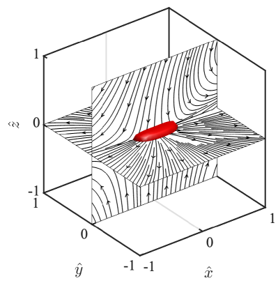
(a)

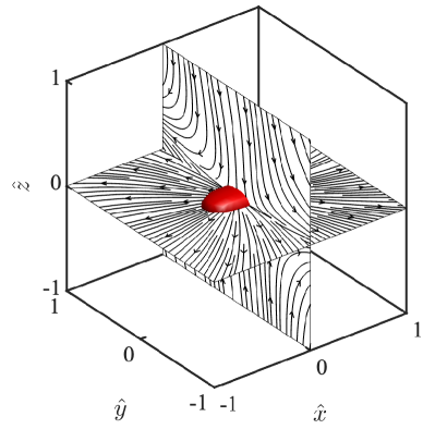
(b)

Figure 6: Streamlines of the conditional-averaged velocity surrounding intense energy cascade events. The streamlines are constrained to the planes (a) $\hat{y}=0$ and $\hat{z}=0$ (b) $\hat{x}=0$ and $\hat{z}=0$. The red isosurface is 50% probability of finding a point belonging to a $\Pi$-structure. The results are for case HIT3 and $r=30\eta$.

The enstrophy pattern ($\{\widetilde{\omega}_{i}\}\{\widetilde{\omega}_{i}\}$) surrounding intense energy transfer events is visualized in figure 7. The red region in figure 7(a,b) represents again the 0.5 probability iso-surface for locating a point belonging to a $\Pi$-structure. The iso-surfaces of the enstrophy field are set at 35% of the maximum value. To facilitate the visualization of enstrophy, the regions for $\hat{z}>0$ and $\hat{z}<0$ are colored in yellow and blue, respectively. The distinctive emerging pattern reveals that the energy cascade occurs between two regions of intense enstrophy. These regions manifest as hairpin-like shapes with opposing orientations that do not overlap with the region where the energy transfer reaches its maximum. The enhanced enstrophy located at $\hat{x}>0$, $\hat{y}>0$, and $\hat{z}>0$, is due the conditional average procedure, which rotates the local frame of reference to favor higher enstrophy within the first quadrant. However, the existence of two enstrophy regions, the specific shapes of these regions, and the absence of overlap with the $\Pi$-structures are not the result of any constraint, but rather a manifestation of the statistical significance of that arrangement.

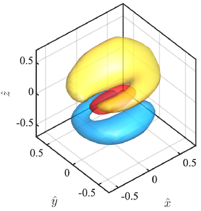
(a)

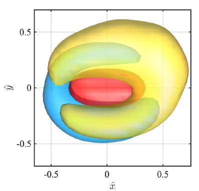
(b)

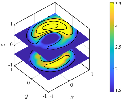
(c)

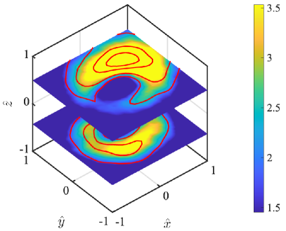
(d)

Figure 7: (a,b) Iso-surface of the probability of finding a point belonging to a $\Pi$-structure equal to 0.5 (red) and conditional-averaged enstrophy $\{\widetilde{\omega}_{i}\}\{\widetilde{\omega}_{i}\}$ at $0.35\times\max\left(\{\widetilde{\omega}_{i}\}^{2}\right)$ at $\hat{z}>0$ (yellow) and $\hat{z}<0$ (blue) is shown in isometric view (a) and $\hat{x}$-$\hat{y}$ projection (b). The results are for case HIT3 and $r=30\eta$. (c,d) Conditional-averaged enstrophy for (c) HIT3 and $r=30\eta$ (color) and HIT2 and $r=30\eta$ (solid black line); (d) HIT3 and $r=30\eta$ (color) and HIT3 and $r=40\eta$ (solid red line). The values are normalized by the standard deviation of $\{\widetilde{\omega}_{i}\}\{\widetilde{\omega}_{i}\}$.

The robustness of the results across Re_λ and filter widths is assessed in figures 7(c) and (d). The figures display the colormap of the conditional-averaged enstrophy in two planes cutting along the hairpin-like structures identified in figures 7(a,b). This approach complements that of figure 7 by eliminating the need to select a threshold to visualize the hairpin-like shape. The solid contours represent the conditional-averaged enstrophy for a different Re_λ (figure 7c) or different filter width (figure 7d). Some small sensitivities can be observed with respect to Re_λ and filter width, likely due to low Reynolds number effects. Nonetheless, the findings are consistent with those from figures 7(a,b) and the same conclusions are drawn.

It is important to note that the hairpin-like structure identified does not imply that instantaneous vortices are shaped in that manner. Rather, it signifies that the irregular arrays of vortices tend to be preferentially located in those regions. Two examples of the instantaneous field surrounding the $\Pi$-structures are depicted in figure 8. It can be seen that intense energy transfer events ($\Pi>\Pi_{\text{\text{rms}}}$, colored in red) are surrounded by areas of high enstrophy ($\widetilde{\omega}_{i}\widetilde{\omega}_{i}$, colored in green). In these particular examples, multiple vortex tubes are positioned closely to the $\Pi$-structures, yet without overlapping in space. Similar instances, consisting of regions of intense $\Pi$ surrounded by distinct regions of intense $\widetilde{\omega}_{i}\widetilde{\omega}_{i}$, were consistently observed. While certain $\Pi$-structures did overlap with vortex tubes, such occurrences were less frequent, in accordance with the results from the conditional-averaged flow.

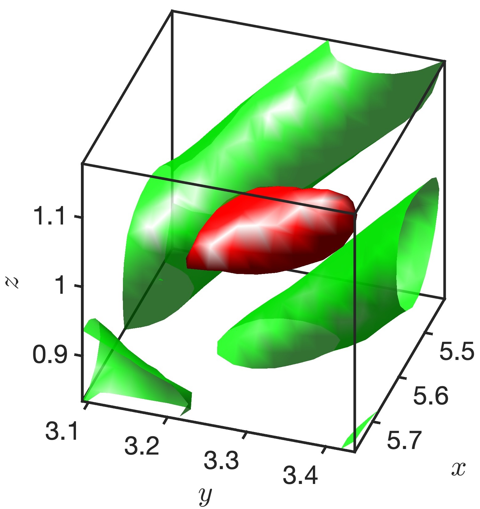
(a)

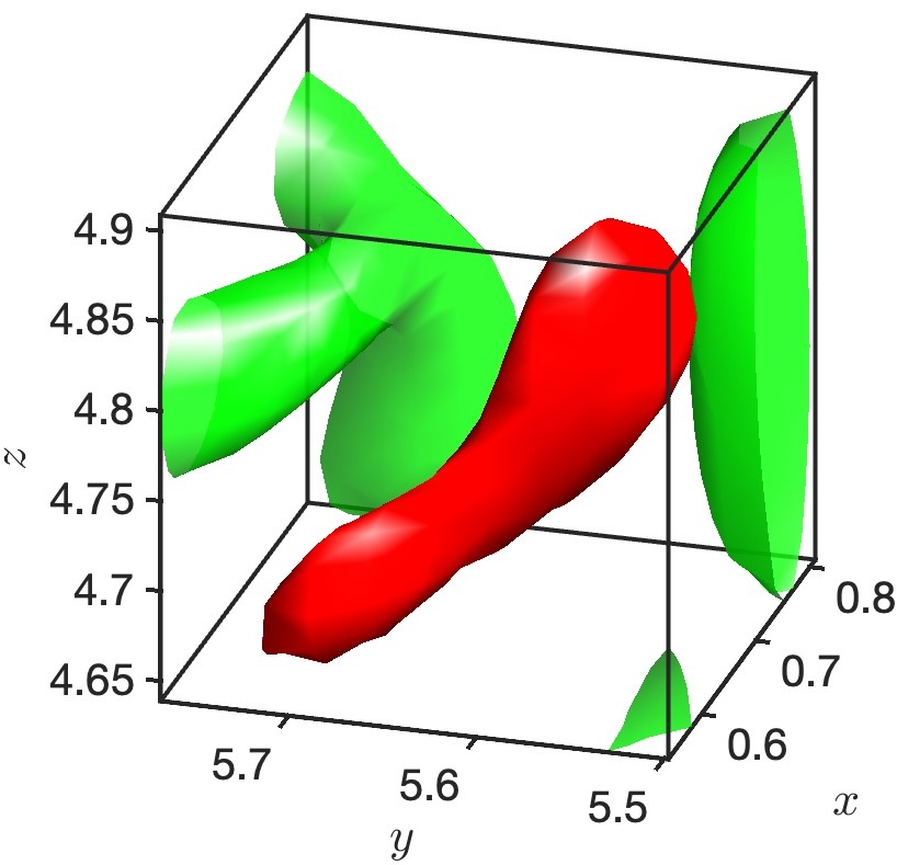
(b)

Figure 8: Examples of instantaneous intense cascade events: iso-surfaces of high transfer regions $\Pi>\Pi_{\text{rms}}$ (red) and high enstrophy regions at $0.025\times\max\left(\widetilde{\omega}_{i}\widetilde{\omega}_{i}\right)$ (green). The results are for case HIT2 and $r=30\eta$.

The results above rely on the assumption that only one type of flow pattern surrounds the intense energy transfer events. However, if patterns with different flow topologies are involved in the cascading process, performing an ensemble average over all the $\Pi$-structures would yield a distorted image of the coherent structure. To assess the possibility of distinct flow patterns contributing to the energy cascade, we divide the samples used to compute $\{\phi\}$ into $n$ groups with the goal of separating instances containing different flow structures. This is achieved by using proper orthogonal decomposition of the velocity field surrounding $\Pi$-structures. Then, the k-means algorithm is applied to place the samples into $n$ groups that minimize within-cluster variances of the three most energetic POD coefficients, denoted by $a_{1}$, $a_{2}$, and $a_{3}$. The POD coefficients and groups are shown in figure 9(a) for the case $n=2$. The conditional-averaged velocity field for each group is portrayed in figures 9(b) and (c). Comparison of the results indicates that both groups share similar flow features despite the division of the samples being targeted to separate velocity patterns. Although not shown, the process was repeated for $n=3$ and $n=4$ groups, which yielded similar conclusions. These findings suggest that the conditional-averaged flow structure outlined in this section is physically relevant and not merely an artifact of the averaging process. Additionally, the results in figure 9 are computed for case HIT2 and $r=30\eta$, which demonstrates that the streamlines in figure 6(a) also hold for different Re_λ and filter width.

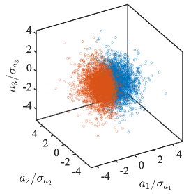
(a)

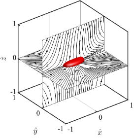
(b)

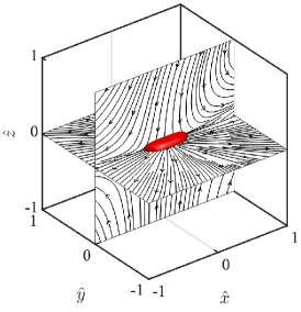
(c)

Figure 9: (a) Point cloud of the three most energetic POD coefficients associated with the velocity field around $\Pi$-structures. The coefficients are normalized by their standard deviation and colored according to the k-mean group they belong to. (b,c) Conditional-averaged shape of transfer object and nearby averaged velocity streamlines for (b) group 1 and (c) group 2. The contours represent 0.5 of the maximum probability of finding a $\Pi$-structure. The streamlines are constrained to the planes $\hat{y}=0$ and $\hat{z}=0$.

3.2 Mechanisms responsible for the inter-scale energy transfer

To gain further insight into the underlying mechanisms driving the energy cascade, we investigate the contributions of the vortex stretching and strain-rate self-amplification in the vicinity of intense energy transfer events. To that end, the kinetic energy transfer $\Pi$ is decomposed into terms ascribed with different mechanisms. The approach adopted here follows the work by Johnson (2020). We outline the key aspects of the decomposition and the reader is referred to the original work for more details. First, let us denote the low-pass Gaussian filter at scale $r$ as $\overline{(\cdot)}^{r}$ such that $\tau_{ij}^{r}=\overline{u_{i}u_{j}}^{r}-\overline{u_{i}}^{r}\overline{u_{j}}^{r}$. In previous sections, we have referred to $\overline{(\cdot)}^{r}$ as $\widetilde{(\cdot)}$. The decomposition of $\Pi$ is grounded on the mathematical relationship between the Gaussian-filter $\tau_{ij}^{r}$ and the diffusion equation

$$12\frac{\partial\tau_{ij}^{r}}{\partial(r^{2})}=\frac{1}{2}\nabla^{2}\tau_{ij}^{r}+\overline{A}_{ij}^{r}\overline{A}_{ij}^{r},\quad\tau_{ij}^{r=0}=0,$$ (4)

where $A_{ij}=\partial u_{i}/\partial x_{j}$ is the velocity gradient tensor and $\nabla^{2}$ is the Laplacian. By solving Eq. (4) and projecting onto $\widetilde{S}_{ij}$, the kinetic energy transfer can be decomposed as

$$\Pi=\Pi_{l}^{S}+\Pi_{l}^{\omega}+\Pi_{nl}^{S}+\Pi_{nl}^{\omega}+\Pi_{nl}^{C}.$$ (5)

The terms above are given by

$$\Pi^{S}_{l} = -\frac{r^{2}}{12}\overline{S}_{ij}^{r}\overline{S}_{jk}^{r}\overline{S}_{ki}^{r},$$ (6)

$$\Pi^{\omega}_{l} = \frac{r^{2}}{48}\overline{\omega}_{i}^{r}\overline{\omega}_{j}^{r}\overline{S}_{ij}^{r},$$ (7)

$$\Pi^{S}_{nl} = -\frac{1}{12}\int_{0}^{r^{2}}\left(\overline{\overline{S}_{ki}^{\theta}\overline{S}_{jk}^{\theta}}^{\phi}-\overline{\overline{S}_{ki}^{\theta}}^{\phi}\overline{\overline{S}_{jk}^{\theta}}^{\phi}\right)\overline{S}_{ij}^{r}\mathrm{d}\theta^{2},$$ (8)

$$\Pi^{\omega}_{nl} = \frac{1}{48}\int_{0}^{r^{2}}\left(\overline{\overline{\omega}_{i}^{\theta}\overline{\omega}_{j}^{\theta}}^{\phi}-\overline{\overline{\omega}_{i}^{\theta}}^{\phi}\overline{\overline{\omega}_{j}^{\theta}}^{\phi}\right)\overline{S}_{ij}^{r}\mathrm{d}\theta^{2},$$ (9)

$$\Pi^{C}_{nl} = -\frac{1}{12}\int_{0}^{r^{2}}\left(\overline{\overline{S}_{ki}^{\theta}\overline{\Omega}_{jk}^{\theta}}^{\phi}-\overline{\overline{S}_{ki}^{\theta}}^{\phi}\overline{\overline{\Omega}_{jk}^{\theta}}^{\phi}\right)\overline{S}_{ij}^{r}\mathrm{d}\theta^{2},$$ (10)

where $\phi=\sqrt{r^{2}-\theta^{2}}$ and $\Omega_{ij}$ is the rate-of-rotation tensor.

The terms $\Pi_{l}^{S}$ and $\Pi_{l}^{\omega}$ (where $l$ denotes ‘local’) are the energy transfer due to local-in-scale interactions of $\overline{S}_{ij}^{r}$ with either the rate-of-strain tensor $\overline{S}_{ij}^{r}$ (i.e., strain self-amplification) or the vorticity vector $\overline{\omega}_{i}^{r}$ (i.e, vortex stretching), respectively. The terms $\Pi^{S}_{nl}$ and $\Pi^{\omega}_{nl}$ (where $nl$ denotes ‘non-local’) are analogous to $\Pi_{l}^{S}$ and $\Pi_{l}^{\omega}$ but correspond to nonlocal-in-scale interactions. Despite the non-local nature of $\Pi^{S}_{nl}$ and $\Pi^{\omega}_{nl}$, it has been shown that they still represent interactions occurring close in scale (e.g., Domaradzki & Rogallo, 1990; Cardesa et al., 2015; Johnson, 2020, 2021; Lozano-Durán & Arranz, 2022). The remaining term, $\Pi_{nl}^{C}$ is also nonlocal in scale and represents energy transfer by the resolved strain-rate tensor acting on the product of strain-rate and vorticity.

The conditional-averaged values for the total energy transfer ($\{\Pi\}$) and its individual contributions ($\{\Pi_{l}^{S}\}$, $\{\Pi_{l}^{\omega}\}$, $\{\Pi_{nl}^{S}\}$, $\{\Pi_{nl}^{\omega}\}$, and $\{\Pi_{nl}^{C}\}$) are calculated following the ensemble average procedure from §2.4. For ease of visualization, the values are plotted in figure 10 along the $\hat{x}$ coordinate, but a similar picture emerges along the other directions, $\hat{y}$ and $\hat{z}$. The results reveal that roughly 85% of the overall energy transfer is primarily attributed to strain-rate self-amplification ($\{\Pi_{l}^{S}\}+\{\Pi_{nl}^{S}\}$), most of which is local (approximately 70%), whereas the contribution of vortex stretching ($\{\Pi_{l}^{\omega}\}+\{\Pi_{nl}^{\omega}\}$) accounts for less than 15%. The dominant role of the local strain-rate self-amplification is consistent with the saddle point topology of the conditional-averaged velocity field from figure 6 and the staggered arrangement between enstrophy and energy transfer from figure 7. Interestingly, the contribution of $\{\Pi_{l}^{\omega}\}$ is essentially zero, implying that vortex stretching acts only from larger-scale strain to slightly smaller-scale vorticity via the term $\{\Pi_{nl}^{\omega}\}$. This phenomenon has been observed in previous studies (Leung et al., 2012; Lozano-Durán et al., 2016; Goto et al., 2017; Yao & Hussain, 2020). The contribution of $\Pi_{nl}^{C}$ is also negligible, at least for the range of filter widths considered. This agrees with the space-time average values of $\Pi_{nl}^{C}$ reported in the literature (Johnson, 2020, 2021). Although some sensitivities can be appreciated across the filter widths (figure 10a) and Reynolds numbers (figure 10b), the conclusions remain robust across the cases investigated.

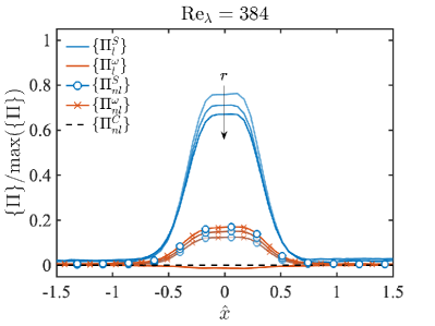
(a)

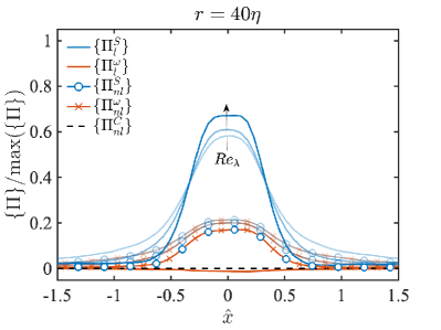
(b)

Figure 10: Conditional-averaged contributions to $\{\Pi\}$ surrounding intense energy-transfer events. The results are shown along the $\hat{x}$ coordinate for $\hat{y}=\hat{z}=0$. The terms are normalized with the maximum of $\{\Pi\}$. (a) Contributions for HIT3 and $r/\eta=20,30$, and $40$ (from light to dark). (b) Contributions for $r/\eta=40$ and HIT1, HIT2, and HIT3 (from light to dark).

4 Conclusions

We have studied the three-dimensional structure of the flow surrounding regions of intense kinetic energy transfer in the inertial range of isotropic turbulence. To that end, the flow velocity was low-passed filtered using a Gaussian filter and the characteristic flow patterns surrounding intense energy transfer events were obtained by conditionally averaging the flow after proper translation, rotation, and re-scaling of the frame of reference.

Our findings have revealed that forward intense energy-transfer events are consistently confined in the high strain-rate region located between two distinct zones of elevated enstrophy resembling hairpin-like shapes. In that region, the local velocity field associated with the energy transfer exhibits a saddle point topology characteristic of strain-dominated regions. Our analysis also highlights that the primary mechanism driving the cascade in these regions is strain self-amplification from local and non-local interactions, which accounts for roughly 85% of the energy transfer, whereas vortex stretching remains below 15%.

The main focus of this work has been on the coherent structure and physical mechanisms involved in the energy cascade. Nonetheless, our results can inform decisions about subgrid-scale (SGS) model developments for large-eddy simulation (LES), especially when the intent is to faithfully represent the processes involved in the cascade. In such situations, the coherent structure of the energy cascade must be consistent with the predominant role of strain-self amplification over vortex stretching. The high strain-rate region created between two distinct zones of elevated enstrophy, as reported here, can serve as a benchmark to evaluate the physical fidelity of SGS models in those contexts. This level of detail is probably not required for SGS models that are aimed at capturing only the general characteristics of the flow, such as mean velocity profiles or mean Reynolds stresses. Another significant implication for SGS modeling stems from the observation that, although 70% of the energy transfer ($\approx\{\Pi_{l}^{S}\}$) is due to local interactions (and thus resolvable by LES), the remaining 30% arises from nonlocal interactions. These latter cannot be resolved by the LES grid and therefore need to be modeled, introducing the challenge of the closure problem.

Our results also suggest that control strategies aiming to enhance or deplete the energy cascade should target the rate-of-strain tensor rather than vorticity. However, this assessment may not be straightforward, as the rate-of-strain tensor and vorticity are kinematically linked, meaning that manipulating one could influence the other. Additionally, any intervention designed to modify the turbulent flow will inevitably affect the dynamics of both the rate-of-strain and vorticity, potentially diminishing the applicability of the coherent structures identified in our study.

Finally, it is worth mentioning that our analysis was based on instantaneous flow snapshots, which only offer a static glimpse into the flow dynamics. Time-resolved data are likely necessary to accurately identify the dynamical relevance of the mechanisms involved in the energy cascade. Future work will be devoted to establishing cause-effect relationships between time-resolved coherent structures and the mechanisms responsible for the transfer of energy among scales.

Declaration of interests

The authors report no conflict of interest.

Appendix A Sensitivity to the threshold for $\Pi$-structures

The $\Pi$-structures are defined as regions satisfying $\Pi>\alpha\Pi_{\text{rms}}$, with the thresholding parameter $\alpha=1$. We tested the sensitivity of the results for $\alpha=1/2$ and $\alpha=2$. The key results, presented in figure 11, show that similar conclusions hold for both $\alpha=1/2$ and $\alpha=2$. This outcome is not surprising, as $\Pi$-structures are merely used as markers to identify regions of the flow where most of the energy transfer occurs. These markers tend to remain in similar locations of the flow across a wide range of thresholding values.

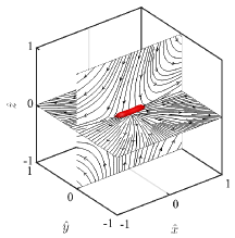
(a)

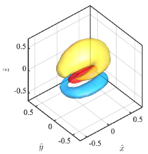
(b)

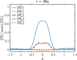
(c)

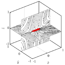
(d)

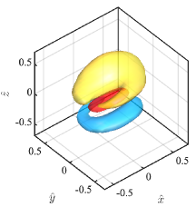
(e)

(f)

Figure 11: Sensitivity to the thresholding parameter to compute $\Pi$-structures. Results for conditional-averaged flow fields for (top row) $\alpha=1/2$ and (bottom row) $\alpha=2$. The results are for HIT3 and $r=30\eta$.

Appendix B Statistical uncertainty

The statistical uncertainty is investigated for case HIT3 and $r=30\eta$. To this end, the number of $\Pi$-structures used to compute the conditional-averaged fields was decreased to one quarter of the total number of samples. The key results of the manuscript are presented in figure 12 for the reduced dataset. Despite the reduction in the number of samples, the qualitative structure of the average flow surrounding intense energy cascade events remains unchanged.

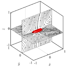
(a)

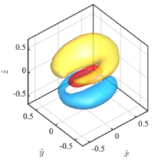
(b)

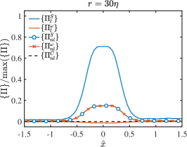
(c)

Figure 12: Statistical uncertainty. Results for conditional-averaged flow fields using one quarter of the total number of samples. The results are for HIT3 and $r=30\eta$.

References

- del Álamo et al. (2004) del Álamo, J. C., Jiménez, J., Zandonade, P. & Moser, R. D. 2004 Self-similar vortex clusters in the turbulent logarithmic region. J. Fluid Mech. 561, 329–358.
- Aluie & Eyink (2009) Aluie, Hussein & Eyink, Gregory L 2009 Localness of energy cascade in hydrodynamic turbulence. ii. sharp spectral filter. Phys. Fluids 21 (11), 115108.
- Aoyama et al. (2005) Aoyama, Tomohiro, Ishihara, Takashi, Kaneda, Yukio, Yokokawa, Mitsuo, Itakura, Ken’ichi & Uno, Atsuya 2005 Statistics of energy transfer in high-resolution direct numerical simulation of turbulence in a periodic box. J. Phys. Soc. Japan 74 (12), 3202–3212.
- Betchov (1956) Betchov, R 1956 An inequality concerning the production of vorticity in isotropic turbulence. J. Fluid Mech. 1 (5), 497–504.
- Bodenschatz (2015) Bodenschatz, Eberhard 2015 Clouds resolved. Science 350 (6256), 40–41.
- Borue & Orszag (1998) Borue, Vadim & Orszag, Steven A 1998 Local energy flux and subgrid-scale statistics in three-dimensional turbulence. J. Fluid Mech. 366, 1–31.
- Brenner et al. (2016) Brenner, Michael P, Hormoz, Sahand & Pumir, Alain 2016 Potential singularity mechanism for the euler equations. Phys. Rev. Fluids 1 (8), 084503.
- Capocci et al. (2023) Capocci, Damiano, Johnson, Perry L., Oughton, Sean, Biferale, Luca & Linkmann, Moritz 2023 New exact betchov-like relation for the helicity flux in homogeneous turbulence. J. Fluid Mech. 963, R1.
- Carbone & Bragg (2020) Carbone, Maurizio & Bragg, Andrew D 2020 Is vortex stretching the main cause of the turbulent energy cascade? J. Fluid Mech. 883, R2.
- Cardesa & Lozano-Durán (2019) Cardesa, J. I. & Lozano-Durán, A. 2019 Inter-scale energy transfer in turbulence from the viewpoint of subfilter scales. Center for Turbulence Research, Annual Research Briefs pp. 195–209.
- Cardesa et al. (2015) Cardesa, José I, Vela-Martín, Alberto, Dong, Siwei & Jiménez, Javier 2015 The temporal evolution of the energy flux across scales in homogeneous turbulence. Phys. Fluids 27 (11), 111702.
- Cardesa et al. (2017) Cardesa, J. I., Vela-Martín, A. & Jiménez, J. 2017 The turbulent cascade in five dimensions. Science 357 (6353), 782–784.
- Cerutti & Meneveau (1998) Cerutti, Stefano & Meneveau, Charles 1998 Intermittency and relative scaling of subgrid-scale energy dissipation in isotropic turbulence. Physics of Fluids 10 (4), 928–937.
- Davidson et al. (2008) Davidson, PA, Morishita, K & Kaneda, Y 2008 On the generation and flux of enstrophy in isotropic turbulence. J. Turb. (9), N42.
- Doan et al. (2018) Doan, NAK, Swaminathan, N, Davidson, PA & Tanahashi, M 2018 Scale locality of the energy cascade using real space quantities. Phys. Rev. Fluids 3 (8), 084601.
- Domaradzki & Rogallo (1990) Domaradzki, J Andrzej & Rogallo, Robert S 1990 Local energy transfer and nonlocal interactions in homogeneous, isotropic turbulence. Phys. Fluids 2 (3), 413–426.
- Domaradzki et al. (2009) Domaradzki, J Andrzej, Teaca, Bogdan & Carati, Daniele 2009 Locality properties of the energy flux in turbulence. Phys. Fluids 21 (2), 025106.
- Dong et al. (2020) Dong, Siwei, Huang, Yongxiang, Yuan, Xianxu & Lozano-Durán, Adrián 2020 The coherent structure of the kinetic energy transfer in shear turbulence. J. Fluid Mech. 892.
- Dong et al. (2017) Dong, S., Lozano-Durán, A., Sekimoto, A. & Jiménez, J. 2017 Coherent structures in statistically stationary homogeneous shear turbulence. J. Fluid Mech. 816, 167–208.
- Eyink (1995) Eyink, Gregory L 1995 Local energy flux and the refined similarity hypothesis. J. Stat. Phys. 78, 335–351.
- Eyink (2005) Eyink, Gregory L 2005 Locality of turbulent cascades. Phys. D: Nonlinear Phenomena 207 (1-2), 91–116.
- Eyink & Aluie (2009) Eyink, Gregory L & Aluie, Hussein 2009 Localness of energy cascade in hydrodynamic turbulence. i. smooth coarse graining. Phys. Fluids 21 (11), 115107.
- Falconer (2004) Falconer, Kenneth 2004 Fractal geometry: mathematical foundations and applications. John Wiley & Sons.
- Goto et al. (2017) Goto, Susumu, Saito, Yuta & Kawahara, Genta 2017 Hierarchy of antiparallel vortex tubes in spatially periodic turbulence at high reynolds numbers. Phys. Rev. Fluids 2, 064603.
- Hamlington et al. (2008) Hamlington, Peter E, Schumacher, Jörg & Dahm, Werner JA 2008 Local and nonlocal strain rate fields and vorticity alignment in turbulent flows. Phys. Rev. E 77 (2), 026303.
- Hof et al. (2010) Hof, Björn, de Lozar, Alberto, Avila, Marc, Tu, Xiaoyun & Schneider, Tobias M. 2010 Eliminating turbulence in spatially intermittent flows. Science 327 (5972), 1491–1494.
- Hong et al. (2012) Hong, J., Katz, J., Meneveau, C. & Schultz, M. P. 2012 Coherent structures and associated subgrid-scale energy transfer in a rough-wall turbulent channel flow. J. Fluid Mech. 712, 92–128.
- Hussain & Duraisamy (2011) Hussain, Fazle & Duraisamy, Karthik 2011 Mechanics of viscous vortex reconnection. Phys. Fluids 23 (2), 021701.
- Johnson (2020) Johnson, Perry L 2020 Energy transfer from large to small scales in turbulence by multiscale nonlinear strain and vorticity interactions. Phys. Rev. Lett. 124 (10), 104501.
- Johnson (2021) Johnson, Perry L 2021 On the role of vorticity stretching and strain self-amplification in the turbulence energy cascade. J. Fluid Mech. 922, A3.
- Kerr (2013) Kerr, Robert M 2013 Swirling, turbulent vortex rings formed from a chain reaction of reconnection events. Phys. Fluids 25 (6), 065101.
- Kolmogorov (1941) Kolmogorov, A. N. 1941 The Local Structure of Turbulence in Incompressible Viscous Fluid for Very Large Reynolds’ Numbers. In Dokl. Akad. Nauk SSSR, , vol. 30, pp. 301–305.
- Kühnen et al. (2018) Kühnen, Jakob, Song, Baofang, Scarselli, Davide, Budanur, Nazmi Burak, Riedl, Michael, Willis, Ashley P., Avila, Marc & Hof, Björn 2018 Destabilizing turbulence in pipe flow. Nat. Phys. 14 (4), 386–390.
- Leung et al. (2012) Leung, T, Swaminathan, N & Davidson, PA 2012 Geometry and interaction of structures in homogeneous isotropic turbulence. J. Fluid Mech. 710, 453–481.
- Lozano-Durán & Arranz (2022) Lozano-Durán, A. & Arranz, G. 2022 Information-theoretic formulation of dynamical systems: Causality, modeling, and control. Phys. Rev. Res. 4, 023195.
- Lozano-Durán et al. (2012) Lozano-Durán, A., Flores, O. & Jiménez, J. 2012 The three-dimensional structure of momentum transfer in turbulent channels. J. Fluid Mech. 694, 100–130.
- Lozano-Durán et al. (2016) Lozano-Durán, A, Holzner, M & Jiménez, J 2016 Multiscale analysis of the topological invariants in the logarithmic region of turbulent channels at a friction reynolds number of 932. J. Fluid Mech. 803, 356–394.
- Lozano-Durán & Jiménez (2014) Lozano-Durán, A. & Jiménez, J. 2014 Time-resolved evolution of coherent structures in turbulent channels: characterization of eddies and cascades. J. Fluid. Mech. 759, 432–471.
- Marusic et al. (2010) Marusic, I., Mathis, R. & Hutchins, N. 2010 Predictive model for wall-bounded turbulent flow. Science 329 (5988), 193–196.
- McKeown et al. (2018) McKeown, Ryan, Ostilla-Mónico, Rodolfo, Pumir, Alain, Brenner, Michael P & Rubinstein, Shmuel M 2018 Cascade leading to the emergence of small structures in vortex ring collisions. Phys. Rev. Fluids 3 (12), 124702.
- Melander & Hussain (1988) Melander, Mogens V & Hussain, Fazle 1988 Cut-and-connect of two antiparallel vortex tubes. Stanford Univ., Studying Turbulence Using Numerical Simulation Databases, 2. Proc. 1988 Summer Program .
- Mininni et al. (2006) Mininni, PD, Alexakis, A & Pouquet, Annick 2006 Large-scale flow effects, energy transfer, and self-similarity on turbulence. Phys. Rev. E 74 (1), 016303.
- Mininni et al. (2008) Mininni, Pablo Daniel, Alexakis, A & Pouquet, A 2008 Nonlocal interactions in hydrodynamic turbulence at high reynolds numbers: The slow emergence of scaling laws. Phys. Rev. E 77 (3), 036306.
- Moisy & Jiménez (2004) Moisy, F. & Jiménez, J. 2004 Geometry and clustering of intense structures in isotropic turbulence. J. Fluid Mech. 513, 111–133.
- Natrajan & Christensen (2006) Natrajan, V. K. & Christensen, K. T. 2006 The role of coherent structures in subgrid-scale energy transfer within the log layer of wall turbulence. Phys. Fluids 18 (6).
- Obukhov (1941) Obukhov, AM 1941 On the distribution of energy in the spectrum of turbulent flow. Bull. Acad. Sci. USSR, Geog. Geophys. 5, 453–466.
- Paul et al. (2017) Paul, I, Papadakis, G & Vassilicos, JC 2017 Genesis and evolution of velocity gradients in near-field spatially developing turbulence. J. Fluid Mech. 815, 295–332.
- Piomelli et al. (1991) Piomelli, U., Cabot, W. H., Moin, P. & Lee, S. 1991 Subgrid-scale backscatter in turbulent and transitional flows. Phys. Fluids 3 (7), 1766–1771.
- Richardson (1922) Richardson, L.F. 1922 Weather Prediction by Numerical Process. Cambridge University Press.
- Richardson (1920) Richardson, Lewis Fry 1920 The supply of energy from and to atmospheric eddies. Proc. Roy. Soc. London. Ser. A 97 (686), 354–373.
- Sagaut & Cambon (2008) Sagaut, Pierre & Cambon, Claude 2008 Homogeneous turbulence dynamics, , vol. 10. Springer.
- Sirovich & Karlsson (1997) Sirovich, L. & Karlsson, S. 1997 Turbulent drag reduction by passive mechanisms. Nature 388, 753 EP –.
- Taylor (1938) Taylor, Geoffrey Ingram 1938 Production and dissipation of vorticity in a turbulent fluid. Proc. Roy. Soc. London. Ser. A 164 (916), 15–23.
- Taylor & Green (1937) Taylor, Geoffrey Ingram & Green, Albert Edward 1937 Mechanism of the production of small eddies from large ones. Proc. Roy. Soc. London. Ser. A 158 (895), 499–521.
- Tennekes et al. (1972) Tennekes, Hendrik, Lumley, John Leask, Lumley, Jonh L & others 1972 A first course in turbulence. MIT press.
- Tsinober (2009) Tsinober, Arkady 2009 An informal conceptual introduction to turbulence. Springer.
- Vela-Martín (2022) Vela-Martín, Alberto 2022 Subgrid-scale models of isotropic turbulence need not produce energy backscatter. J. Fluid Mech. 937, A14.
- Vela-Martín & Jiménez (2021) Vela-Martín, Alberto & Jiménez, Javier 2021 Entropy, irreversibility and cascades in the inertial range of isotropic turbulence. J. Fluid Mech. 915, A36.
- Veynante & Vervisch (2002) Veynante, Denis & Vervisch, Luc 2002 Turbulent combustion modeling. Prog. Energy Combust. Sci. 28 (3), 193 – 266.
- Yao & Hussain (2020) Yao, Jie & Hussain, Fazle 2020 A physical model of turbulence cascade via vortex reconnection sequence and avalanche. J. Fluid Mech. 883, A51.
- Young & Read (2017) Young, Roland M. B. & Read, Peter L. 2017 Forward and inverse kinetic energy cascades in jupiter’s turbulent weather layer. Nat. Phys. 13, 1135 EP –.
- Zhou (1993a) Zhou, Ye 1993a Degrees of locality of energy transfer in the inertial range. Phys. Fluids 5 (5), 1092–1094.
- Zhou (1993b) Zhou, Ye 1993b Interacting scales and energy transfer in isotropic turbulence. Phys. Fluids 5 (10), 2511–2524.